motion planning for autonomous vehicles - cvut.cz

Motion Planning for Autonomous Vehicles

Michal Cap

Autonomous Car Architecture

Figure from Brian Paden

Motivation

Motivation

Driving in highly structured environments;

Video by Ricco831

MotivationDriving in urban environments:

Video by Mobileye

Motivation

Picture by

Rachmaninoff

Driving in unstructured cluttered environments:

Problem Informally

Motion Planning:

The problem of finding a collision-free motion for a robot from given start pose to given destination pose.

Planning for a Conventional Car

Obstacles from a priori map

Obstacles from sensors

Free space

Constraints on path:● Starts at current position● Ends at goal position● Robot does not collide with obstacles● Respect limited turning-radius

start pose

goal pose

1

3

2

4

Formalization

Workspace: (x,y)

W⊂R2

Obstacles space (Wobst)

Free workspace (Wfree)

Configuration of Robot

x

y(0,0,0)


x

y(0,0,π/4)


x

y(5,0,π/4)

Configuration Space: (x,y,θ)

X ⊂ R2 x [-π,+π]

(0,0,0)

(5,3,π/4)

(0,5,π)

θ

x

y

θ=π

y=5

θ=π/4

x=5

y=3

O c1

c2c3

c1

c2

c3

Free Configuration:



(-1,0,π/4)

Collision Configuration:



(1,0,π/4)

Free Configuration Space

Let R(x) be the region occupied by robot at configuration x ∊ X.

The set of all collision-free configurations is

Xfree = {x : x ∊X and R(x) ⊂Wfree}


Slice of Xfree for θ=π/4:

Obstacle space (Wobst)

Free configuration space (Cfree)

Collision configurations

Free Configuration Space -- Illustration


θ=0





θ=⅛ π





θ=¼ π





θ=⅜ π





θ=½ π




Path in Configuration Space

σ(α): [0,1] → X

θ

x

y

x=5

y=5θ=π/4

O

c1

c2

c1x

y

c2

x=5

y=5

O

Trajectory in Configuration Space

π(t): [0,T] → X

θ

x

y

x=5

y=5θ=π/4

O

c1

c2

c1 x

y

c2

t=0t=2 t=6

t=8

t=0

t=2

t=6t=8

Path Planning Problem Formulation

arg min J(𝝈) subject to𝝈(0) = xinit

𝝈(1) ∊ Xgoal

𝝈(𝛼) ∊ Xfree ∀𝛼 ∊ [0,1]

Can be formulated as an optimization problem over all paths in configuration space:

● 𝝈(𝛼) is a continuous function [0,1] → X ● J(𝝈) is a cost functional● xinit is the initial configuration of the robot● Xgoal is the set of goal configurations● Xfree is the free configuration space

Holonomic System

Holonomic system:(no differential constraints)


𝝈(1) = Xgoal

𝝈(𝛼) = Xfree ∀𝛼 ∊ [0,1]D(𝝈(𝛼),𝝈’(𝛼),𝝈’’(𝛼),...) ∀𝛼 ∊ [0,1]

Nonholonomic system:(differential constraints)


𝝈(1) = Xgoal

𝝈(𝛼) = Xfree ∀𝛼 ∊ [0,1]

E.g., bound on path curvature k can be enforced as |𝝈’(𝛼) 𝝈’’(𝛼)|/|𝝈’(𝛼)|3 < k.

Nonholonomic System

Complexity of Path Planning

● Path planning “Piano Movers problem” is PSPACE-hard [Reif ‘79]

● Complete (non-optimal) algorithms for exist [Canny ‘88] but have running time exponential in dimension of configuration space.

Solution Techniques for Path Planning Problem

● Variational Methods● Graph-search Methods

○ Cell decomposition○ Visibility graph○ Sampling-based roadmap construction○ Tree of motion primitives

● Incremental Search Methods○ RRT: Rapidly-exploring Random Trees○ RRT*: Optimal Rapidly-exploring Random Trees

Properties of Path Planning Methods

An algorithm is

● Complete: if it finds valid path or detect non-existence of thereof in finite time.● Optimal: if it find optimal path in finite time.

● Anytime: if it can be terminated at any point of the execution, but the path quality improves with computation time

● Probabilistically Complete: if the probability that the algorithm finds valid solution goes to 1 with running time.

● Asymptotic Optimal: if it returns a sequence of solutions converging to an optimal solution.

Trajectory Planning Problem Formulation

arg min J(π) subject toπ(0) = xinit

π(T) ∊ Xgoal

π(t) ∊ Xfree (t) ∀t ∊ [0,T]D(π(t),π’(t),π’’(t),...) ∀t ∊ [0,T]

Useful for

● Dynamic constraints● Dynamic obstacles

Can be formulated as optimization in the space of trajectories over time interval [0,T] in configuration space:

Solution Techniques for Trajectory Planning Problem

● Variational Methods● Convert to Path Planning in Space-Time:

trajectory planning in (x,y,θ) =>

path planning in (x,y,θ,t) + diff. constraints

Variational TechniquesAka Trajectory optimization, Optimal control, etc.

● Non-linear optimization● Path is represented as a spline● Position of control points is optimized

Variational Techniques

Obstacles are modelled as high-cost regions


Find gradient


Move the control points in the direction of negative gradient


Repeat until convergence

Variational TechniquesPros:● Efficient● Widely applicable

Cons:● Only local convergence

○ Incomplete○ Locally optimal

Notes:● Used in for local path optimization within CMU’s car ‘Boss’.

Graph-based MethodsCfree

Graph(Roadmap)

Discretization

Graph search (Dijsktra/A*/D*)

Graph Path

Path in Cfree

Concatenate edges

Vertices: selected configurations in CfreeEdges: path segments in Cfree connecting two given vertices

Roadmap

Cell Decomposition● A method for building roadmaps in 2d polygonal environments

Cell DecompositionPros:● Complete● Generalizes to higher dimensions and beyond polygonal models

Cons:● Only holonomic systems● Suboptimal

Visibility Graph

● Polygonal environment● Circular robot

Visibility Graph

● Compute collision-free configuration space

Visibility Graph

● Vertices: corners of obstacles, start, and goal. Edge if two vertices “see” each other.

Visibility Graph

● Complete graph

Visibility Graph

● Graph search to obtain shortest path in graph

Visibility GraphPros:● Efficient: O(n2)● Exact optimal

Cons:● Optimality guarantee only for 2-d environments and circular robot● Only for holonomic systems and polygonal models

Sampling-based Roadmap Construction

Generate roadmap by:

● 1. Sampling the free configuration space○ Deterministically○ Randomly

● 2. Connecting nearby samples○ All neighbors closer than distance r○ K-nearest neighbors


Deterministic Sampling (Sukharev Grid)


Probabilistic Roadmap

r


Connecting Samples

r


Finding Path

Steering: Connecting the SamplesSampling-based methods rely on steering function.● Steer(x,y) returns a feasible path segment between configuration x and y.● Steering function respects kinematic and dynamic constraints, but does not

consider obstacles.● Often obtained by simulating a dynamic model of the vehicle.

Steering for Duckiebot

Rotate

Straight

Rotate

Dubins Path: Steering for vehicle moving forward

Picture by Steven LaValle.

start

goal start

goal

● Car that moves only forward. ● The shortest path for can be computed analytically● It consist of three path segments: sharpest-possible turn left (L), right (R) or straight (S). ● Total six templates: {LRL, RLR, LSL, LSR, RSL, RSR}

Reeds-Shepp Path: Steering for Car Moving Forwards and Backwards.

Picture by Steven LaValle.

start

goal

● Car that can move both forward and backwards.● Up to 5 segments: {R+,R-, L+, L-, S+, S-}. ● 46 templates.

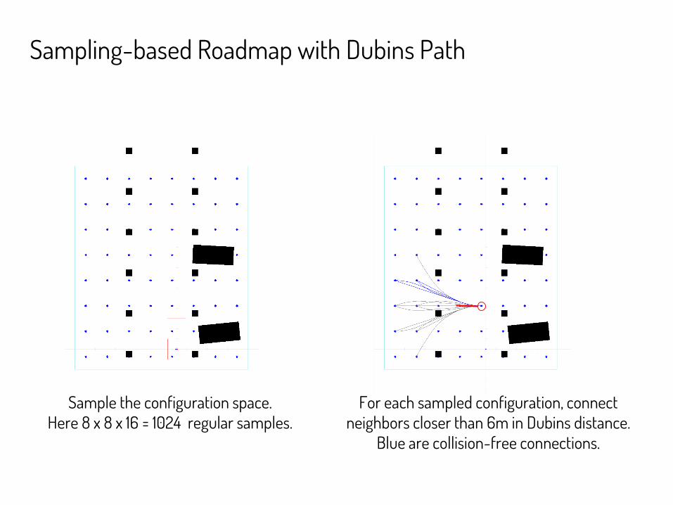
Sampling-based Roadmap with Dubins Path

Sample the configuration space. Here 8 x 8 x 16 = 1024 regular samples.

For each sampled configuration, connect neighbors closer than 6m in Dubins distance.

Blue are collision-free connections.


Resulting roadmap Graph searched using Dijkstra/A*, we obtain a feasible path for the

vehicle.

start

goal

Choosing Connection Radius● How to choose connection radius?

○ too small: roadmap will be disconnected○ Too large: to many computationally intensive

● PRM* [Karaman 2011]: for asymptotic optimality, chose connection radius as a function of number of samples of graph:

○ O(log n) connections attempted at each iteration○ Maintains asymptotic optimality with O(n log n) complexity

Sampling-based Roadmap ConstructionPros:● Handle differential constraints● Model agnostic● Multiquery● PRM/PRM* - asymptotic optimality guarantee

Cons:● Completeness and optimality achieved only up to discretization resolution● Need exact steering

Motion Primitives

A discrete set of of maneuvers that the vehicle can execute from each configuration:

Recursive Application of Motion Primitives

Recursive Application of Motion Primitives

● Can be computed “lazily” during A* search.

Start expanding motion primitives from current configuration.

Use Dijkstra/A* to find the shortest path to the desired region in the tree.

Lattice generating motion primitives

● Some motion primitives generate regular lattice.

90-deg turns generate lattice 89-deg turns do not generate lattice.

Motion PrimitivesPros:● No need for exact steering function● Can handle differential constraints● Model agnostic

Cons:● Completeness and optimality achieved only up to discretization resolution● Single-query

Notes:● Used in CMU’s Boss and Stanford’s Junior during DARPA Urban Challenge

Incremental Search● Graph-based methods plan on a fixed resolution.

○ => Path might be suboptimal○ => They may fail to find solution

● Main idea: ○ Incrementally grow a tree rooted at initial configuration to explore the

reachable region of the configuration space.○ Once first branch reaches goal region, return the branch as the first solution.○ Keep reporting the shortest branch found so far

● Anytime

Rapidly-exploring Random Tree (RRT)

start

goal

Rapidly-exploring Random Tree (RRT)Pros:● Anytime● Handles differential constraints● Does not need exact steering● Probabilistic completeness guarantee (shown for some variants of the algorithm)● Demonstrated good performance in high-dimensional systems

Cons:● Suboptimal● Single-query

Notes:● Used in MIT Talos Urban Challenge Vehicle

Optimal Rapidly-exploring Random Tree (RRT*)

start

goal

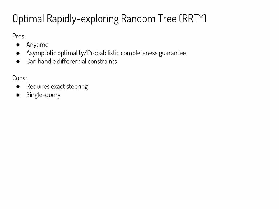
Optimal Rapidly-exploring Random Tree (RRT*)Pros:● Anytime● Asymptotic optimality/Probabilistic completeness guarantee● Can handle differential constraints

Cons:● Requires exact steering● Single-query

Summary

● Motion planning is needed in complex driving situations● Path Planning vs. Trajectory Planning● Different solution approaches

○ Variational○ Graph-based○ Incremental

motion planning for autonomous vehicles - cvut.cz

Documents