morphable surface models - ucrcshelton/papers/docs/match.pdf · morphable surface models christian...

Morphable Surface Models ∗

Christian R. SheltonMassachusetts Institute of Technology

February 23, 2000

Abstract. We describe a novel automatic technique for finding a dense corre-spondence between a pair of n-dimensional surfaces with arbitrary topologies. Thismethod employs a different formulation than previous correspondence algorithms(such as optical flow) and includes images as a special case. We use this correspon-dence algorithm to build Morphable Surface Models (an extension of MorphableModels) from examples. We present a method for matching the model to new surfacesand demonstrate their use for analysis, synthesis, and clustering.

1. Introduction

The goal of this paper is to describe a general method for learning mod-els of surface classes without user intervention. The technique works onsurfaces of any dimension embedded in a Euclidean space and is notspecific to any particular modality. The Morphable Surface Models ofthis paper are a generalization of Morphable Models (described below).

The key problem in building such models is finding correspondencesbetween surfaces. We define a correspondence to be a relation frompoints on one object to their matching points on the other object. Inimages such relations are often called flow fields and have found a widevariety of uses. Here we extend the notion from images to surfaces ingeneral1 and employ the correspondence algorithm to build MorphableSurface Models.

The remainder of this introduction describes previous work in Mor-phable Models and surface matching. Section 2 describes the correspon-dence algorithm by first describing the minimization problem, thenthe algorithm for performing the minimization, and finally the roleof surface simplification. In section 3, we describe how to use the

∗ This paper describes research done within the Center for Biological and Com-putational Learning in the Department of Brain and Cognitive Sciences and atthe Artificial Intelligence Laboratory at the Massachusetts Institute of Technology.This research is sponsored by grants from the National Science Foundation, ONRand Darpa. Additional support is provided by Eastman Kodak Company, Daimler-Chrysler, Siemens, ATR, AT&T, Compaq, Honda R&D Co., Ltd., Merrill-Lynch,NTT and Central Research Institute of Electric Power Industry.

1 A gray scale image can be described as a surface or height-field. Color imagescan similarly be described (now in 5-dimensional space instead of 3-dimensionalspace).

c© 2000 Kluwer Academic Publishers. Printed in the Netherlands.

main.tex; 23/02/2000; 19:01; p.1

2 Christian R. Shelton

correspondence algorithm to build models. To do so, we introduce amethod for matching the models to surfaces, an inner product on thespace of correspondences, and how to apply bootstrapping. Section 4describes experimental results obtained by building models of varioustypes of surfaces and gives an illustration of the steps of the correspon-dence algorithm. Lastly, section 5 gives some conclusions and possibleextensions.

1.1. Morphable Models

It is known that linear models in the image space are generally poormodels for classes of images. Such a model describes members of theclass as alpha-blendings of the examples. This in general produces poorresults. Unless the images align pixel-for-pixel, the alpha-blending oftwo images will not produce a third image in the same class of images:instead the synthesized image will be two “ghosts” of the combinedimages.

The difficulty lies in the fact that every pixel of the new image isa linear combination of the pixels at the same location in the otherimages. These other pixels may not be related to each other and thustaking a linear combination of them will produce nothing of worth.However, if we can match “corresponding” pixels across the set ofexample images, then linear combinations of these corresponding pixelswill work better as a model (Beymer and Poggio, 1996).

For this paper we define a correspondence to be a relation betweentwo objects that maps each of the points on one object to its “cor-responding” point on the other object (where we appeal to intuitionfor the definition of corresponding). For images, a correspondence issimply a flow field from one image to another. Morphable Models areconstructed from a set of example images by finding flow fields from anarbitrary base example image to all of the other example images. Asa generative model, the output is the base image warped by a linearcombination of the flow fields. The parameters of the model are theweights of the linear combination. The pixel values aligned by thecorrespondences may also be combined linearly to produce an imagethat is not only a combination of the “shapes” of the examples (theflow fields) but also the “texture” of the examples (the pixel values).

In this paper, we consider a more general morphable model. Insteadof dealing only with images, we allow the objects to be surfaces of arbi-trary dimension embedded in Euclidean space. Images are a particularexample of such a surface (a gray-scale image is a two-dimensionalmanifold in three-dimensional space: one dimension for each imageaxis and one dimension for intensity). Thus we will build a general

main.tex; 23/02/2000; 19:01; p.2

Morphable Surface Models 3

correspondence technique for any pair of surfaces (replacing the flowfield algorithm for images) and, from that, a general technique forbuilding morphable models of arbitrary surfaces. At the end of thispaper, we will show some simple examples of the uses of MorphableSurface Models.

1.2. Related Work

Morphable Models have been applied mainly to images. Jones and Pog-gio (1998) has a good description of their image method and relatedimage-based techniques. We would refer to their introduction as thebest description of the Morphable Model literature. Briefly, the resultthat new views of a 3D object can be synthesized linearly from threesample views (Ullman and Basri, 1991; Shashua, 1992) spurred thecreation of models of image classes as linear combinations of examples(Poggio and Vetter, 1992; Vetter and Poggio, 1995; Beymer et al.,1993; Beymer and Poggio, 1996).

Since Jones and Poggio (1998), Vetter et al. (1997) developed abootstrapping technique (used and redescribed in this paper) for betterautomatic construction of Morphable Models. Recently, Blanz and Vet-ter (1999) extended Morphable Models to 3D shapes by describing theshape as its projection onto a 2D surface (which can then be unrolledand treated as an image). From there they were able to use MorphableModels to reconstruct 3D shape from a single view. Kang and Jonesalso have used such a projection technique to constrain reconstruction.

Active Appearance Models (Cootes et al., 1998) also try to matchimages but require user specified correspondences. Deformable Inten-sity Surfaces (Nastar et al., 1996) treat images as surfaces and use anautomatic matching technique not dissimilar to the one described here.However, the topology of the surface is essentially limited to that of agrid. Active Contour Models (or Snakes) (Kass et al., 1988; McInerneyand Terzopoulos, 1995) are also similar to the work in this paper. Theyoperate on surfaces of arbitrary dimensions and topologies. However,they are used to match a surface to gradients in volumetric data insteadof to other surfaces.

In this paper we have used the term “n-dimensional surface” to meana surface with n orthogonal tangent vectors at every point. In ActiveContour Models this phrase is taken to imply that the surface lies inan n-dimensional space (and the surface itself has a dimensionality lessthan n). We have used the phrase “dimensionality of the embeddedspace” to denote such a quantity.

The difficult part of building a morphable model and many othermodeling techniques is finding correspondences. We believe this is the

main.tex; 23/02/2000; 19:01; p.3


first paper to propose an algorithm for automatically finding surfacecorrespondences between surfaces with arbitrary topologies directly.The energy minimization method here is based on that described in(Shelton, 1998), has certain similarities to elastic networks (Durbinand Willshaw, 1987), and has energy terms related to the surface re-construction work of Hoppe and others (Hoppe et al., 1992; Hoppeet al., 1993).

2. Matching Surfaces

To build a Morphable Surface Model, we must first be able to findthe correspondences between the example surfaces. This will serve asthe foundation for model construction algorithm. We define an energyfunction over all possible correspondence relations for which smallervalues indicate better correspondences. We will then give an algorithmfor finding a minimum of this energy function which will hopefullycorrespond to a good match according to the metric encoded in theenergy function. Crucial to the practical success of this minimizationis the mesh simplification described in section 2.4.

2.1. Energy Function

Let C be a function which maps points on one surface, A, to arbitrarypoints in space. In order for C to be a good correspondence from A toB we propose it must satisfy three properties:

1. Similarity: For every point a on the surface A, C(a) should be nearor on the surface B.

2. Structure: C should distort the surface A as little as possible. Putdifferently, C(A) should be as structurally similar to A as possible.

3. Prior Information: C should represent a plausible deformation ofthe surface.

The first property states that C should be a correspondence and actu-ally match points on A to points on B. The second says that such amatching should not be arbitrary, but rather should attempt to keepthe structure of the first surface. This will hopefully force matching ofsimilar substructures from A to those of B and preserve our intuitivenotion of correspondence. The last term serves to enforce prior knowl-edge about valid shapes (for example, we may wish to penalize surfaceswhich cross a lot and are very unsmooth as being unlikely results fromany correspondence).

main.tex; 23/02/2000; 19:01; p.4


Our energy function will therefore have the following form:

E(C) = Esim(C) + αEstr(C) + βEpri(C) (1)

Esim measures how closely C matches points on A to points on B.To ease notation, let us define PX (q) to be the point on the surface Xclosest to the point q. We will then define Esim as

Esim(C) =

∫

C(A)‖c− PB(c)‖2 dc+

∫

B

∥∥b− PC(A)(b)∥∥2

db (2)

This is the sum of the integrals over each surface of the squared distancefrom points on that surface to the other surface.

The definitions of the remaining two terms of the energy functionwill depend on prior information we have about surfaces. More sophis-ticated methods of measuring the distortion of the surface could bedeveloped and used. However, we have found that connecting springsbetween points on the surface to be sufficient. In particular we willuse “directional” springs that prefer their original orientation (not justtheir original length). There are two reasons for this choice: First, theytend to minimize buckling of the surface more than “regular” springs(which actually encourage it) and second, they lead to a nice form forthe minimization algorithm since they are quadratic. For a directionalspring connecting the two points p and q, the energy of that springunder the correspondence C is

Eds(p, q, C) =‖(p− q)− (C(p)−C(q))‖2

‖p− q‖ (3)

To create a tight surface and an energy function which does not dependon the parameterization of the surface, we let

Estr(C) =

∫

AEds(a, a+ da,C) (4)

This corresponds to placing directional springs continuously over theentire surface.

If we let Es(p, q, C) be similarly defined for a normal spring of restlength 0,

Es(p, q, C) =‖C(p)− C(q)‖2‖p− q‖ (5)

in order to penalize discontinuous surfaces, we define Epri to be

Epri(C) =

∫

AEs(a, a+ da,C) (6)

main.tex; 23/02/2000; 19:01; p.5


The three terms of E(C) do not play equal roles. The first, Esim,must be zero for C to be a true correspondence. The second, Estr,exists to guide and select among C functions which set the first termto zero. The last term, Epri, serves to smooth out any noise whichmay arise due to inaccurate models or an inability to find the truecorrespondence; as a prior over surfaces, it models the fact that veryunlikely correspondences should be discarded in favor of more likelyones which perhaps do not satisfy the other requirements as well.

Thus, the weighting of the various terms in E(C) will be set asfollows: α will be initially large to enforce a good correspondence.Over time, it will be reduced to allow the algorithm to drive Esimto zero. β will be set to a small constant value which is inverselyproportional to our confidence in our model and ability to find thecorrect correspondence.

2.2. Practical Instantiation of the Energy Function

The energy function as described in the previous section is not practicalto use. The integrals, for most surfaces, are intractable to compute. Inthis paper, we consider only piece-wise linear surfaces and can thereforemake a number of useful simplifications. For a d-dimensional surface(meaning that there are d orthogonal tangent vectors at every pointon the surface), the surface can be defined as an ordered collection ofvectors (the positions of the vertices of the surface) and a set of linearpatches connecting d+1 vectors from the collection. Hoppe et al. (1993)gives a more mathematically concrete definition of such a structure (atuple of the vertex positions and a simplicial complex). A triangulatedmesh is an example of such a 2-dimensional surface.

The integrals in Esim are easily and well approximated by a uniformstochastic sampling of their respective surfaces. Thus, we have

Esim =1

n

∑

c∈Sn(C(A))

‖c− PB(c)‖2 +1

n

∑

b∈Sn(B)

∥∥b− PC(A)(b)∥∥2

(7)

where Sn(X ) is a set of n points sampled from the surface X .

Esim is therefore independent of the parameterization of the surface.In other words, given two different tessellations of the same surface,Esim will not change. We have not yet found similarly parameter-independent approximations of Estr and Epri which yield simple algo-rithms. Instead we approximate both by connecting adjacent vertices inthe surface description with the appropriate springs. Since the springsdefined above are normalized by length, a given straight length of springwill be independent of how it is cut (i.e. how many sections are usedto describe it). Yet, past 1-dimensional surfaces, the energy terms as

main.tex; 23/02/2000; 19:01; p.6


a whole will not be independent of the tessellation used. However, wehave found it to work well in practice.

Estr =1

|Ad(A)|∑

(p,q)∈Ad(A)

Eds(p, q, C) (8)

Epri =1

|Ad(A)|∑

(p,q)∈Ad(A)

Es(p, q, C) (9)

where Ad(A) is the set of all pairs of adjacent vertices in the surfacetessellation A.

2.3. Energy Minimization

Just as we limited the surface to be piece-wise linear, we will limit thecorrespondence function to be piece-wise linear. In particular, we willallow C to take arbitrary values at the vertices of A and require it tobe a linear interpolation of the vertex values along the faces of A. Thismeans that applying C to A simply involves applying the elements ofC to their respective vertices of A: no structural or topological changesneed be made to A.

With this parameterization of C, Estr and Epri are clearly quadratic

in the elements of C. However, Esim is not so well behaved due to theunsmooth nature of the function P (whose first derivative is discontin-uous). We therefore turn the algorithm into a dual optimization. First,we compute PB(c) and PC(A)(b) for all of the a and b samples. We then

fix them at which point Esim becomes quadratic (and thus E(C) isquadratic) and we can solve this minimization for C in closed form.This gives a new set of positions for the vertices from which we canrepeat the sampling, calculation of the closest points, and values of C.

To be more concrete about the algorithm, let us first note that anypoint on the surface of X can be described as a convex combinationof the positions of the vertices of X . For vertices (such as p and q

in Estr and Epri), the combination coefficients are all 0 except for a

single 1. For points internal to a face (such as c or PC(A)(b) in Esim),the coefficients are all zero except for d + 1 non-zero elements (whichsum to 1 due to convexity) corresponding to the d + 1 vertices of theface on which the point is located. These coefficients are sometimescalled the barycentric coordinates of the point (Hoppe et al., 1993).The barycentric coordinates are invariant to the transformations weare allowing for C. That is, the barycentric coordinates of a in A arethe same as the barycentric coordinates of C(a) in C(A).

We will now add the notation that any variable with an overscoreis not a Euclidean vector in the embedded space of the surface, but a

main.tex; 23/02/2000; 19:01; p.7


barycentric coordinate vector (a vector of the coefficients of the previ-ous paragraph) with respect to the appropriate surface. Furthermore,we will let the matrix A be the matrix whose columns are the vectors ofthe positions of the vertices of A. B will be similarly defined for B andC will be the matrix whose columns are the positions of the verticesof A under the correspondence. Thus if A has vA vertices, B has vBvertices, and they are embedded in a D-dimensional space, A and Care D × vA and B is D × vB.

By expanding E(C) by using the relationships b = Bb, a = Aa, andC(a) = Ca, we can then write the whole energy function as

E(C) =1

n

∑

c∈Sn(C(A))

∥∥Cc−BPB(Cc)∥∥2

+1

n

∑

b∈Sn(B)

∥∥Bb− CPC(A)(Bb)∥∥2

+α

|Ad(A)|∑

(p,q)∈Ad(A)

1

‖A(p− q)‖ ‖(C −A)(p− q)‖2

+β

|Ad(A)|∑

(p,q)∈Ad(A)

1

‖A(p− q)‖ ‖C(p− q)‖2

(10)

where, to carry the overscore notation further, S is a set of barycentriccoordinate vectors (of points sampled uniformly over the surface asbefore) and P is the barycentric coordinate vector of the closest pointon the surface. Note that if we fix a sampling over each surface and wefix the values of P (they actually depend on C, but we are fixing them),

then every term of E is of the form wi ‖Cci − di‖2 (wi is a scalar, C isa matrix of vertex positions, ci is the barycentric coordinate vector forthe constraint, and di is the target position).

This optimization can be solved by converting it to a sparse linear-least squares problem separately for each dimension (Hoppe et al.,1993). However, we have found that an improvement can be made atthis stage before conversion to a linear system. At each step of theminimization, points are sampled from each surface and for each point,the closest point on the other surface is found. Then, E is minimizedassuming that the goal is to minimize the distance from each sampledpoint to the found closest point. However, a better match might befound if, instead of insisting that the point match the closest point, werelax and allow the point to match any position on the closest face. Thisis closer to our goal of allowing the point to match anywhere on thesurface. Since the closest face is bounded, we have to approximate this

main.tex; 23/02/2000; 19:01; p.8


by minimizing the distance from the point to the plane of the closestface.

Thus, instead of minimizing wi∥∥Cai −BP i

∥∥2for points sampled

from A or wi∥∥CP i −Bbi

∥∥2for points sampled from B, we are min-

imizing wi∥∥TiCai − TiBP i

∥∥2and wi

∥∥TiCP i − TiBbi∥∥2

where Ti is amatrix which projects out the tangent directions for the face on Binvolved in the ith constraint. Depending on whether the sampled orprojected point on B falls on a vertex, edge, or face, there could be from0 to d orthogonal tangent vectors at that point on B. If we enumeratethem as the unit length vectors ti,1, . . . , ti,m,

Ti = I −∑

m

ti,mtTi,m (11)

(If instead of allowing the point to be anywhere on the plane of theface, we wish to penalize moving from the closest point slightly, we canplace a coefficient between 0 and 1 in front of the sum in the aboveequation thus resulting in a slightly different distance metric.)

Since the constraints now have terms of the form (TiCai)T (TiCai),

they cannot be converted into a sparse linear least-squares system inde-pendently for each dimension. Instead, we must solve for all dimensionssimultaneously (unless all Ti matrices are diagonal). However, with abit of careful manipulation, we can derive a different sparse system tosolve.

Our energy function now has the form

E =∑

i

wi(TiCai − qi)2 (12)

where wi, Ti, ai, and qi are different depending on the constraint: forthe first n constraints, wi = 1

n , ai is the barycentric coordinate vectorof a point sampled from A, qi is the closest point on B to this sampledpoint, and Ti is the tangent matrix at the point qi. For the second nconstraints, wi = 1

n , qi is a sampled point on B, Ti is the tangent matrixto this point, and ai is the barycentric coordinate vector of the point onA closest to qi. For the next |Ad(A)| constraints, wi = α

|Ad(A)|‖A(p−q)‖ ,Ti = I, qi is the difference between the positions of the two vertices inA, and ai is the difference between the barycentric coordinate vectorsof the two vertices (a vector with one 1 and one −1). Finally, the last|Ad(A)| constraints are exactly the same as the previous |Ad(A)| exceptthe α is replaced by β in wi and qi = 0.

For the proper definition of the matrix Ri (a function of Ti andai) and the vector c (a function of C) as derived below, this can be

main.tex; 23/02/2000; 19:01; p.9


converted into

E =∑

i

(Ric− qi)2 (13)

which is a classic least-squares problem with the solution

c =

(∑

i

RTi Ri

)−1∑

i

RTi qi (14)

First we will define c as shown pictorially below to be the vector ofthe components of the matrix C:

cT =[C1,1 · · · CD,1 C1,2 · · · CD,2 · · · · · · C1,N · · · CD,N

](15)

where N is the total number of constraints.We now define Ri as:

(Ri)j,D(k−1)+l = (Ti)j,l(ai)k (16)

which means that Ri has the block form:

Ri =[(ai)1Ti (ai)2Ti · · · (ai)NTi

](17)

(remember that (ai)k is the kth element of the vector ai and thus ascalar). It can easily be shown from here that Ric = TiCai. We nowhave a simple linear least-squares problem with the solution shown inequation 14.

A nice property of this formulation is that Ri is sparse. Only upto d + 1 elements of ai may be non-zero and thus only a maximum ofd+ 1 of the blocks of Ri are non-zero. Many of the Ti matrices are theidentity matrix (for all of the spring constraints) and thus many moreof the elements of Ri will be zero for these constraints. So, while RTi Riis a DN ×DN matrix, only a maximum of D2(d + 1)2 elements of itwill be non-zero. Furthermore, these D×D blocks that make up RT

i Rican only be non-zero for blocks that correspond to adjacent vertices inA. Thus the matrix

∑iR

Ti Ri that needs to be inverted (or at least for

which an LU-decomposition needs to be found) in equation 14 is verysparse. It is symmetric and on every row, a maximum of Dg elementsare non-zero (where g is the maximum outgoing degree of any vertexin A). The solution therefore can be computed efficiently using sparseinversion techniques such as conjugate gradient descent (Press et al.,1992).

main.tex; 23/02/2000; 19:01; p.10


2.4. Surface Simplification

A vital component in our minimization algorithm is the simplificationof the surface descriptions. Attempting to minimize the energy functionas described in the previous section directly on the original models Aand B can result in severely suboptimal local minima and long runningtimes. To combat both of these problems, we first perform a sequenceof surface simplifications. For A we produce the sequence of surfaces{A0,A1, . . . ,AlA} and for B we produce the sequence {B0,B1, . . . ,BlB}where A0 and B0 are the original input surfaces and X i+1 is a meshapproximating X with half the complexity of X i. Complexity can beany measure; in this case we use the number of vertices. lA and lB aredetermined by setting a threshold on the maximum distance from thesimplified surface to the original surface. A single threshold works wellfor all similar models.

The computer graphics literature has a number of algorithms thatcan be used to produce simpler meshes approximating an input mesh.Heckbert and Garland (1997) gives a good review of the major algo-rithms of the field. We have implemented and used progressive meshes(Hoppe, 1996) and quadric error metrics (Garland and Heckbert, 1997)and both provide qualitatively the same performance when used inour algorithm on the types of surfaces described in the experimentalsection of this paper. However, our implementation of Garland’s andHeckbert’s quadric error metrics runs faster and so the results reportedin this paper use that algorithm.

Once we have the sequence of simplified surfaces, we begin with thetwo simplest surfaces (AlA and BlB ) and use the energy minimizationtechnique from the previous section to find a correspondence betweenthe two surfaces. We then use the found correspondence to initializethe starting position for finding the correspondence between the nexttwo surfaces in each sequence (i.e. AlA−1 and BlB−1). We continue inthis manner until we finally compute the correspondence between A0

and B0 (the original input surfaces). If lA 6= lB, then at some pointone of the two sequences will run out of more complex surfaces. Atthat point, we just continue to use the most complex surface for theshorter sequence until the algorithm has matched all of the surfaces inthe other sequence and finished.

At the base level, the correspondence is initialized to be the ver-tex positions of AlA : no movement of A. At each new step when amore complex model is introduced for A, we must find a positionof the vertices of Ai based on the correspondence found for Ai+1.Because Ai and Ai+1 could have arbitrarily different geometries or

main.tex; 23/02/2000; 19:01; p.11


even topologies2, for every vertex a of the surface Ai, we let CAi(a) =a+CAi+1(PAi+1(a))−PAi+1(a). More informally, we take every vertexof the new, more complex surface, and project it to the simpler surface.We compute the corresponding point to that projection point based onthe old coarse correspondence. We then take the implied motion of thatpoint (the difference between the projected point the correspondenceat the projected point) and add that to the vertex to give the initialcorrespondence at the vertex of the more complex surface.

2.5. Polygon Reduction verses Image Pyramids

In some optical flow and other image matching algorithms, a similarsimplification is used on the images to produce a pyramid of imagesfrom which the correspondence can be computed in a coarse-to-finemanner. Gaussian or Laplacian pyramids are usually the method ofchoice where each simpler layer in the set is a blurred down-sampledversion of the previous (or possibly the derivative thereof). We arguethat the polygon reduction described above is fundamentally differentin that the surface is simplified in a data-dependent fashion. Gaussianand Laplacian pyramids are constructed by applying the same linearfilters to the image regardless of the image. Polygon reduction producessimpler surfaces by careful consideration of the shape of the surface.This insures a more faithful representation of the surface especially atthe simplest levels which means that the computations done at coarsestlevels have much more bearing on the final output thereby leading tofewer local minima and faster computation because less work needs tobe undone.

As pointed out in Hoppe (1996), mesh simplification can be seen asa (potentially lossless) compression technique. It is not surprising thatcompression can be used to obtain a good representation for matching.If we assume that both surfaces are collections of features drawn from arandom (but structured) distribution, we would expect a compressionalgorithm to be able to find common substructures and reduce themin the same way thus allowing for easier matching. Finding the bestmethod for compression and the best features for learning are oftensimilar problems. We can view the polygon reduction stages of thealgorithm as implicit feature detectors.

2 For the two algorithms we tested, progressive meshes and quadric error met-rics, and many other mesh simplification algorithms, the simplification is done bycollapsing edges and thus the vertices of Ai can be mapped to the vertices of Ai+1.However, after removing half of the vertices such a mapping can be misleading andwe would like this algorithm to be independent of the method used to obtain thesimplified surfaces.

main.tex; 23/02/2000; 19:01; p.12


3. Morphable Surface Models

Now that we have an algorithm for finding correspondences betweensurfaces, we turn to building Morphable Surface Models. We are givenm surfaces, {A1,A2, . . . ,Am} and we fix one of them as the base surface(without loss of generality, assume this is the one labeled A1). We nowfind the correspondences between A1 and all of the other surfaces.This produces a set of correspondences {C1, C2, . . . , Cm} (where C1 istrivially computed and the rest describe how to warp A1 to each of theother surfaces in the set).

These correspondences can be combined in a convex combination toproduce a new warping of the base surface. If Ξ = {ξ1, ξ2, . . . , ξm} arethe convex combination coefficients (

∑i ξi = 1), then we define this

new warping in the obvious way,

WΞ(a) =∑

i

ξiCi(a) (18)

where WΞ(a) is the new position of the point a from the base meshin the model whose parameters have been set to Ξ. This restricts thenew warping to lie in the m−1-dimensional space of these m warpings.Clearly there is a slight bias in this model relative to the arbitrary choiceof the base surface (since correspondence calculations as describedabove are not invariant to the ordering of the two surfaces). However,for classes of similar objects with the same or similar topologies, thisbias is small.

To remove the condition that the sum of the ξi parameters must be1, we will assume that the model parameters have been centered (wewill translate the space to a “center point” making any scaling of awarping a valid warping). By this we mean that an origin model hasbeen set to warping when all ξi = 1

m and the correspondence vectorshave been changed from the absolute positions of the vertices to therelative difference between the vertex position for the correspondenceand the vertex position of this origin model. Mathematically, we definean origin as O(a) =

∑i

1mCi(a) and then define new “displacement”

correspondences C ′i(a) = Ci(a) − O(a) and associated parameters ξ′iwhich do not now need to sum to 1. This means that W is now

W ′Ξ(a) = O(a) +∑

i

ξ′iC′i(a) (19)

From now on, we will drop the prime notation and assume that allmodels have been described in this fashion to eliminate the convexconstraint on the ξ’s.

main.tex; 23/02/2000; 19:01; p.13


3.1. Matching Models to Surfaces

We can now formulate an algorithm for finding the parameters ofa morphable model so that the shape of the model best matches agiven surface, B (this surface is not necessarily one of the ones used toconstruct the model). We again pose this as an energy minimizationproblem with the following energy term:

Em(Ξ) =

∫

A1

‖WΞ(a)− PB(a)‖2 da+

∫

B

∥∥b− PWΞ(a)(b)∥∥2

db+ λ∑

i

ξi

(20)

This minimizes the difference between points from the model’s sur-face and their closest points on the target surface and vice-versa. Wehave also added a term penalizing high coefficient values. This reflectsour intuition that the model will not be a good one far away fromthe surfaces used to construct it. If our model has been whitened asdescribed in section 3.3, then this penalty is analogous to assuming aGaussian prior in correspondence space.

Again, the minimization of Em is difficult due to the integrals, sowe will approximate them with sums of sampled points yielding

Em(Ξ) =1

n

∑

a∈Sn(O(A1))

‖W (a)− PB(W (a))‖2

+1

n

∑

b∈Sn(B)

∥∥PW (A)(b)− b∥∥2

+ λ∑

i

ξi

(21)

Just as before, we can minimize this function by alternating betweenfinding the closest points to sampled points from the opposite surfaceand fixing these points to find Ξ by solving a linear-least squares prob-lem. In this case, we do not minimize the distance to the plane, but justthe distance to the projected point for simplicity. By taking derivativesof Em with respect to Ξ while keeping the values of PB(W (a)) con-stants (pretending they don’t depend on Ξ) and the values of PW (A)(b)as linear functions of Ξ (pretending their barycentric coordinates arefixed), the second half of the minimization has the solution:

Ξ = (A+ 2nλI)−1 q (22)

where

Aij =∑

k

Ci(ak)TCj(ak) (23)

qi =∑

k

Ci(ak)T bk (24)

main.tex; 23/02/2000; 19:01; p.14


for k ranging over the terms of both sums of equation 21. ak is the pointon model’s surface (sampled for the first n values of k and projectedfrom a point on B for the second n) and bk is the associated point onB (projected from a point on the model’s surface for the first n valuesof k and sampled for the second n).

3.2. Inner Products of Correspondence

In order to use bootstrapping (Vetter et al., 1997; Jones and Poggio,1998) for building models in a more robust manner (section 3.3), weneed to define an inner product over the space of correspondences. Itmight seem that if we simply stack all of the components of the corre-spondence vectors at each vertex into a large vector, we could use thedot product of these vectors as the inner product of the correspondencespace. However, this definition is sensitive to the parameterization ofthe base surface. As an example, if we keep the base surface the sameand the correspondences the same but subdivide some of the faces of thebase surface (so we have the same surface described in a different way),we end up with a different inner product: we have lengthened the vectorof vertex positions (although the new components are dependent on theold ones) and therefore magnified the importance of the correspondenceat the faces we subdivided.

To solve this problem, we define the inner product between twocorrespondences in a parameter-independent fashion,

< Ci, Cj >=

∫

A1

Ci(a)TCj(a) da (25)

We would now like to find a tractable method for computing thisintegral for piece-wise linear surfaces. For concreteness, we will takethe example of 2-dimensional surfaces which are therefore composedof triangles. The analysis and resulting answer generalize to arbitrarydimensional surfaces.

The above integral, for the case of 2-dimensional piece-wise linearsurfaces, becomes the sum of integrals of Ci(a)TCj(a) over triangles.We know that Ci(a) is a linear function of a over the triangle patch(and similarly with Cj(a)). Therefore, the integral of the dot productof these two vectors is a quadratic function of position taken over the

main.tex; 23/02/2000; 19:01; p.15


triangle. The following equality holds and can be verified easily.

∫

4x0x1x2

Ci(x)TCj(x) dx =

1

12area(4x0x1x2)

[2∑

k=0

Ci(xk)TCj(xk) +

2∑

k=0

2∑

l=0

Ci(xk)TCj(xl)

]

(26)

To allow us to use normal vector packages, we derive a new vectorrepresentation for a correspondence whose dot-product in the usualvector sense is exactly this inner product. Let VA be the set of allvertices of A, FA be the set of all faces of A, {f0, f1, f2} be the verticesof the face f , and F (v) be the set of faces adjacent to the vertex v.

< Ci, Cj >=∑

f∈FA

∫

fCi(x)TCj(x) dx

=∑

f∈FA

[1

12area(f)

[2∑

k=0

Ci(fk)TCj(fk) +

2∑

k=0

2∑

l=0

Ci(fk)TCj(fl)

]]

=∑

v∈VA

∑

f∈F (v)

1

12area(f)Ci(v)TCj(v)

+∑

f∈FA

1

12area(f)

2∑

k=0

Ci(fk)T

2∑

k=0

Cj(fk)

=∑

v∈VA

√∑

f∈F (v) area(f)

12Ci(v)

T √∑

f∈F (v) area(f)

12Cj(v)

+∑

f∈FA

[√area(f)

12

2∑

k=0

Ci(fk)

]T [√area(f)

12

2∑

k=0

Cj(fk)

]

(27)

which implies that, if D is the dimensionality of the embedded space,the inner product can be represented as a dot product between twovectors whose first D×VA components are the positions of the verticesof the surface multiplied by the square root of the sum of the areas ofthe adjacent faces and whose last D× FA components are the sums ofthe positions of the vertices of each of the fA faces multiplied by thesquare root of the area of the face.

main.tex; 23/02/2000; 19:01; p.16


3.3. Building a Model

Now that we have an inner product for correspondences, we can use thebootstrapping algorithm described in Vetter et al., Jones and Poggio(1997, 1998) to build the model robustly. Usually the method de-scribed above (where we take each of the surfaces and compute itscorrespondence to the base surface) will work fine. However, since thecorrespondence algorithm is not perfect, occasionally some parts of thecorrespondence will be off. If we have a large number of surfaces tobe incorporated, we can correct for this problem in many cases. Thebootstrapping algorithm is

1. Let M be the model. Initialize it as just the base surface (thus onlyone correspondence)

2. Repeat the following until the model has reach the desired level offlexibility:

a) for each input surface:

i) Match the current model to the surface (as in section 3.1)yielding an approximation to the input surface: W (a)

ii) Find the correspondence from the base surface to the ap-proximation, W (a) (as in section 2): C(a)

iii) Let Ci(a) = W (C(a)).

b) Center the correspondences found in the previous step (as de-scribed in the beginning of section 3) and create the data matrixM whose columns are the centered correspondences (in thevector representation of section 3.2).

c) Perform singular value decomposition on M yielding UDV T .

d) Retain only those columns of U with the largest singular values,increasing the number of parameters of the model (each columnof U is an axis of correspondence space). Scale each column byits singular value.

In this algorithm, we successively build a more and more flexiblemodel. Each time we use the old model to match the input surfacesand give an easier starting point for the correspondence routines. Wethen find and keep, via singular value decomposition, the axes of ourspace with largest variance since they are likely to be “real” surfacechanges and not due to noise in our correspondence algorithm.

Since we are scaling the axes by the standard deviation of the cor-respondences (in step (d)), we have whitened the data. This supportsthe

∑i ξi log-prior term in the matching energy function of section 3.1.

main.tex; 23/02/2000; 19:01; p.17


4. Experimental Results

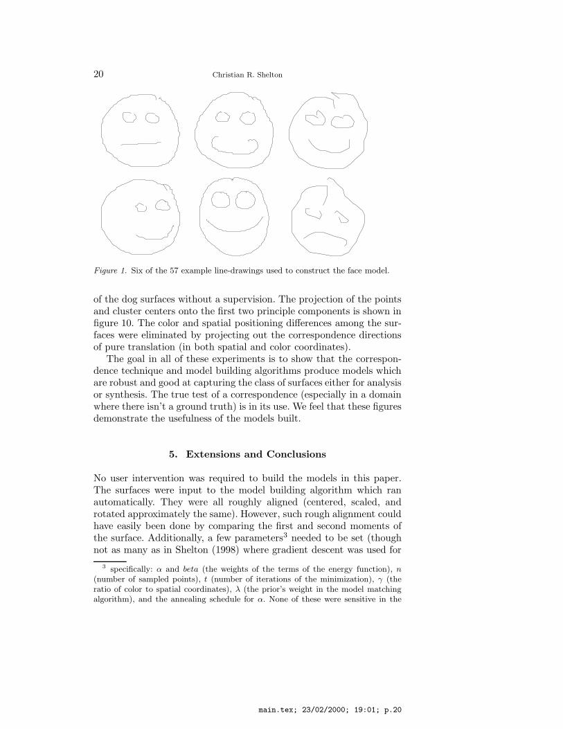
We report results of running the model building algorithm on three col-lections of surfaces. Figure 1 shows a few examples from a collection ofhand-drawn “smiley faces.” These surfaces are (one-dimensional) linesembedded in the (two-dimensional) plane. They were created using atablet input device which sampled the pen position over time. Theexample faces have between 66 and 407 line segments each, with mostsurfaces having about 100 segments. All faces were composed of fourseparate open curves and thus had the same topology; however thistopological equivalence was not used in the matching.

These types of line drawings are very difficult for conventional opti-cal flow algorithms: if the surfaces were converted to images, the spatialderivatives would be zero almost everywhere. A simple matching ofclosest points also fails dramatically because of the variation in theposition of the eyes and mouth. It results in matching portions of someeyes and mouths to the large head circle. The structure term plays acrucial role.

We ran the bootstrapping algorithm on 57 faces for 23 iterationsproducing a model with 23 parameters. Figure 2 shows the major axesof variation captured by the model (the principal components of thelast iteration of the bootstrapping algorithm).

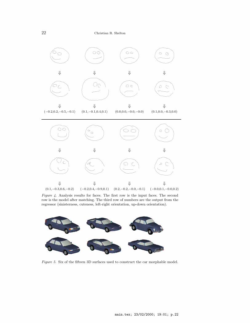
We then asked two people to rank each face on four attributes(friendly vs. sinister, ugly vs. cute, left-looking vs. right-looking, anddown-looking vs. up-looking). We created a radial-basis function (RBF)regressor (Bishop, 1995) mapping those four attributes to the dimen-sions of the face model. From that mapping, we automatically generatedthe results shown in figure 3. Similarly, we used an RBF to create thereverse mapping (from parameters to attributes). Figure 4 shows theresults of matching eight faces not used in creating the model and thenestimating the attributes from the resulting model parameters.

Secondly, we constructed a surface model of cars from 15 computergraphics surfaces (6 of which are shown in figure 5). These models havedifferent topologies. All of the cars have five closed surfaces represent-ing the body and tires. Some additionally have either open or closedsurfaces representing the bumpers and side mirrors. Between 1270 and10568 triangles define each surface. Color is represented by three extradimensions (red, green, and blue). Thus, these shapes are 2D surfacesembedded in six-dimensional space. This 6D representation allows thealgorithm to trade-off matching color verses matching shape. In previ-ous Morphable Model work with images, the variations in shape haddifferent model parameters than those of texture (or color). This wouldbe analogous to separating every correspondence in the model into two

main.tex; 23/02/2000; 19:01; p.18


correspondences (one that had only non-zero spatial components andone that had only non-zero color components). We have chosen notto do so here and instead our results insist that the color and surfacechanges be dependent. Thus a given correspondence represents a changein the surface shape and surface color.

We ran the bootstrapping algorithm to completion (15 rounds, addingone additional parameter per round). The resulting principle compo-nents are shown in figure 6. Given that only 15 example surfaces wereused and the high dimensionality of the problem (over 6000 numbersto represent one surface), we feel these capture the natural variationsin car bodies well. The bounding boxes on the cars were normalized,so the first eigenvector well captures the difference between small andlarge car shapes. The second could be characterized as a “sporty” verses“boxy” axes. The third and fourth make distinctions in the tail-lightsand rear windows.

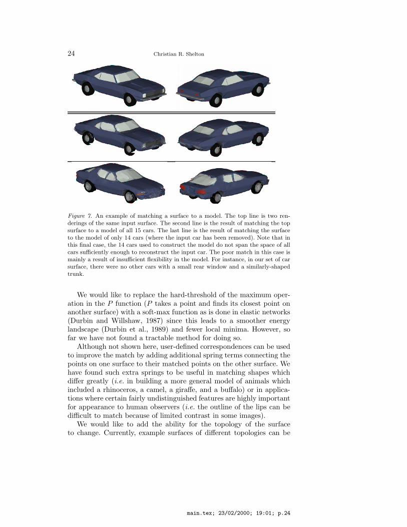
The results from the matching procedure from section 3.1 are shownin figure 7. The first line is the input car to be matched. The secondline is the model matched to the input. The third line is the model withthe input car removed matched to the input. The difference betweenthe second and third lines is mainly due to limited size of the model. Asthere are only 14 other cars, they do not completely span the space ofall cars and thus were not able to exactly match the input. There wereonly two other “sporty” two-seater cars and no other car had such largeside or rear windows. Thus it was impossible for the model to representthe input shape as the learned examples did not cover that portion of“car shapes.”

The wheels in most of the car correspondences are a problem. Be-cause they are round, the matching algorithm tends to add a bit of ran-dom rotation to the correspondences. Rotation correspondence fields donot add linearly and thus the wheel representations are not as crisp asthe rest of the vehicle (the wheels tend to collapse). This is essentially amismatch between the polygonal representation and the round surface.

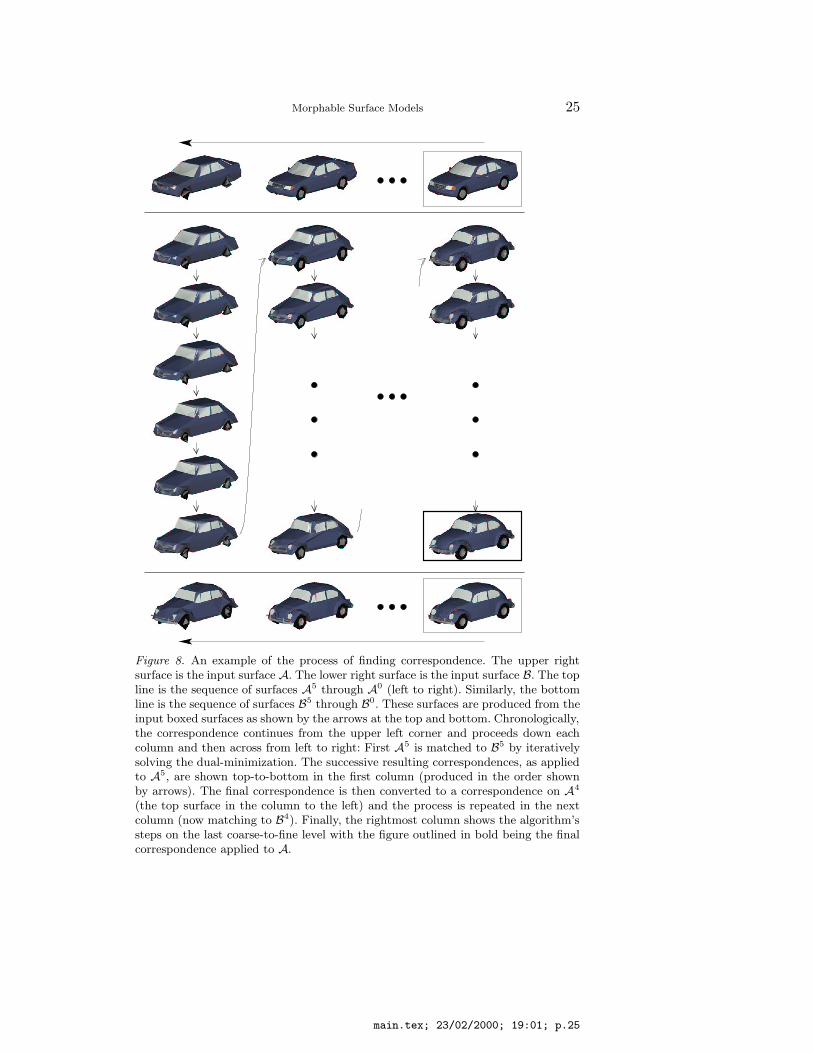
To visually demonstrate the correspondence algorithm, figure 8 showsthe results of each step of the algorithm run on two car surfaces. Wethink this clearly shows the iterative refining of the solution from coarseto fine resolution. Notice that most of the gross changes are done at thecoarse level where the number of free variables (positions of vertices)are minimal. This helps to prevent overfitting.

Finally, to demonstrate the use of these correspondences as a metric-space, we took the animal surfaces of figure 9 and built a morphablemodel. Using the distance metric implied by the vector representationof section 3.2, we clustered the examples using the k-means algorithm(Bishop, 1995). This produced one cluster of the cat surfaces and one

main.tex; 23/02/2000; 19:01; p.19


Figure 1. Six of the 57 example line-drawings used to construct the face model.

of the dog surfaces without a supervision. The projection of the pointsand cluster centers onto the first two principle components is shown infigure 10. The color and spatial positioning differences among the sur-faces were eliminated by projecting out the correspondence directionsof pure translation (in both spatial and color coordinates).

The goal in all of these experiments is to show that the correspon-dence technique and model building algorithms produce models whichare robust and good at capturing the class of surfaces either for analysisor synthesis. The true test of a correspondence (especially in a domainwhere there isn’t a ground truth) is in its use. We feel that these figuresdemonstrate the usefulness of the models built.

5. Extensions and Conclusions

No user intervention was required to build the models in this paper.The surfaces were input to the model building algorithm which ranautomatically. They were all roughly aligned (centered, scaled, androtated approximately the same). However, such rough alignment couldhave easily been done by comparing the first and second moments ofthe surface. Additionally, a few parameters3 needed to be set (thoughnot as many as in Shelton (1998) where gradient descent was used for

3 specifically: α and beta (the weights of the terms of the energy function), n(number of sampled points), t (number of iterations of the minimization), γ (theratio of color to spatial coordinates), λ (the prior’s weight in the model matchingalgorithm), and the annealing schedule for α. None of these were sensitive in the

main.tex; 23/02/2000; 19:01; p.20


mean face

−2σ +2σ −2σ +2σ

↔ ↔

↔ ↔

↔ ↔

Figure 2. The first 6 eigenvectors of the face model scaled by ±2 standard deviationsshown applied to the average face.

(1, 0, 0, 0) (0, 1,−1, 0) (0, 0,−1, 0) (0,−0.5, 1,−1)⇓ ⇓ ⇓ ⇓

Figure 3. Results of fitting a radial-basis function network to mapping from fourattributes (sinisterness, cuteness, left-right orientation, up-down orientation) to mor-phable model parameters. Four example outputs from settings of the attributes areshown.

minimization). We found that running a few test correspondences tofind the correct order of magnitude for the parameters was all that wasnecessary.

For its generality, we feel that the energy function described pro-duces good results. However, in domains where prior knowledge about

least and very easy to set except for the annealing schedule which we had to tunedifferently for each set of surfaces.

main.tex; 23/02/2000; 19:01; p.21


⇓ ⇓ ⇓ ⇓

⇓ ⇓ ⇓ ⇓(−0.2,0.2,−0.5,−0.1) (0.1,−0.1,0.4,0.1) (0.0,0.0,−0.0,−0.0) (0.1,0.0,−0.3,0.0)

⇓ ⇓ ⇓ ⇓

⇓ ⇓ ⇓ ⇓(0.1,−0.3,0.6,−0.2) (−0.2,0.4,−0.9,0.1) (0.2,−0.2,−0.0,−0.1) (−0.0,0.1,−0.0,0.2)

Figure 4. Analysis results for faces. The first row is the input faces. The secondrow is the model after matching. The third row of numbers are the output from theregressor (sinisterness, cuteness, left-right orientation, up-down orientation).

Figure 5. Six of the fifteen 3D surfaces used to construct the car morphable model.

main.tex; 23/02/2000; 19:01; p.22


mean car

−2σ +2σ

↔

↔

↔

↔

Figure 6. The first four eigenvectors of the car model. Each eigenvector is shownapplied to the average model scaled by ±2 standard deviations. The other eigenvec-tors have similar forms. We show the cars from this view since the back of the cartends to have the most variation.

surface deformations is available, better results could certainly be ob-tained by modifying the Estr and Epri terms. Preliminary results withusing this algorithm as a replacement for optical flow are promis-ing (Shelton, 1998): the polygon reduction produces large triangles intextureless areas leading to easy matching where traditionally opti-cal flow algorithms have had problems. Yet, this algorithm makes noassumptions about the images matched.

main.tex; 23/02/2000; 19:01; p.23


Figure 7. An example of matching a surface to a model. The top line is two ren-derings of the same input surface. The second line is the result of matching the topsurface to a model of all 15 cars. The last line is the result of matching the surfaceto the model of only 14 cars (where the input car has been removed). Note that inthis final case, the 14 cars used to construct the model do not span the space of allcars sufficiently enough to reconstruct the input car. The poor match in this case ismainly a result of insufficient flexibility in the model. For instance, in our set of carsurface, there were no other cars with a small rear window and a similarly-shapedtrunk.

We would like to replace the hard-threshold of the maximum oper-ation in the P function (P takes a point and finds its closest point onanother surface) with a soft-max function as is done in elastic networks(Durbin and Willshaw, 1987) since this leads to a smoother energylandscape (Durbin et al., 1989) and fewer local minima. However, sofar we have not found a tractable method for doing so.

Although not shown here, user-defined correspondences can be usedto improve the match by adding additional spring terms connecting thepoints on one surface to their matched points on the other surface. Wehave found such extra springs to be useful in matching shapes whichdiffer greatly (i.e. in building a more general model of animals whichincluded a rhinoceros, a camel, a giraffe, and a buffalo) or in applica-tions where certain fairly undistinguished features are highly importantfor appearance to human observers (i.e. the outline of the lips can bedifficult to match because of limited contrast in some images).

We would like to add the ability for the topology of the surfaceto change. Currently, example surfaces of different topologies can be

main.tex; 23/02/2000; 19:01; p.24


Figure 8. An example of the process of finding correspondence. The upper rightsurface is the input surface A. The lower right surface is the input surface B. The topline is the sequence of surfaces A5 through A0 (left to right). Similarly, the bottomline is the sequence of surfaces B5 through B0. These surfaces are produced from theinput boxed surfaces as shown by the arrows at the top and bottom. Chronologically,the correspondence continues from the upper left corner and proceeds down eachcolumn and then across from left to right: First A5 is matched to B5 by iterativelysolving the dual-minimization. The successive resulting correspondences, as appliedto A5, are shown top-to-bottom in the first column (produced in the order shownby arrows). The final correspondence is then converted to a correspondence on A4

(the top surface in the column to the left) and the process is repeated in the nextcolumn (now matching to B4). Finally, the rightmost column shows the algorithm’ssteps on the last coarse-to-fine level with the figure outlined in bold being the finalcorrespondence applied to A.

main.tex; 23/02/2000; 19:01; p.25


Figure 9. Surfaces used for constructing an animal model (this model has also beenused for psychophysics experiments (Riesenhuber and Poggio, 1999; Riesenhuberand Poggio, 2000)). Clustering using the k-means algorithms (for k = 2) producedthe top row as one cluster and the bottom row as another cluster. This nicelycorresponds to cats and dogs.

Figure 10. Plotting the six surfaces in correspondence space (projected onto the twoaxes of largest variance). The × markers are the cat surfaces and the circles are thedogs. The stars represent the cluster centers found.

main.tex; 23/02/2000; 19:01; p.26


used to create a model. However, all of the surfaces produced by thatmodel will all have the topology of the base surface. McInerney and Ter-zopoulos (1995) describe a method for allowing the topology of snakesto change during the matching process. Combining this idea with themesh reduction algorithm of Popovic and Hoppe (1997), which allowstopology changes, might provide for a more flexible surface model.

References

Beymer, D. and T. Poggio: 1996, ‘Image Representations for Visual Learning’.Science 272, 1905–1909.

Beymer, D., A. Shashua, and T. Poggio: 1993, ‘Example Based Image Analysis andSynthesis’. A.I. Memo 1431, Artificial Intelligence Laboratory, MassachusettsInstitute of Technology.

Bishop, C. M.: 1995, Neural Networks for Pattern Recognition. Oxford: ClarendonPress.

Blanz, V. and T. Vetter: 1999, ‘A Morphable Model For The Syntheis Of 3D Faces’.In: Computer Graphics Proceedings, SIGGRAPH’99. pp. 187–194.

Cootes, T. F., G. J. Edwards, and C. J. Taylor: 1998, ‘Active Appearance Models’.In: Proceedings of the European Conference on Computer Vision, Vol. 2. pp.484–498.

Durbin, R., R. Szeliski, and A. Yuille: 1989, ‘An Analysis of the Elastic Net Approachto the Traveling Salesman Problem’. Neural Computation 1, 348–358.

Durbin, R. and D. Willshaw: 1987, ‘An analogue approach to the travelling salesmanproblem using an elastic net method’. Nature 326(16), 689–691.

Garland, M. and P. S. Heckbert: 1997, ‘Surface Simplification Using Quadric ErrorMetrics’. In: Computer Graphics Proceedings, SIGGRAPH’97. pp. 209–216.

Heckbert, P. S. and M. Garland: 1997, ‘Survey of Polygonal Surface SimplificationAlgorithms’. Technical report, Carnegie Mellon University. to appear.

Hoppe, H.: 1996, ‘Progressive Meshes’. In: Computer Graphics Proceedings,SIGGRAPH’96. pp. 99–108.

Hoppe, H., T. DeRose, T. Duchamp, J. McDonald, and W. Stuetzle: 1992, ‘SurfaceReconstruction from Unorganized Points’. In: Computer Graphics Proceedings,SIGGRAPH’92. pp. 71–78.

Hoppe, H., T. DeRose, T. Duchamp, J. McDonald, and W. Stuetzle: 1993, ‘MeshOptimization’. In: Computer Graphics Proceedings, SIGGRAPH’93. pp. 19–26.

Jones, M. J. and T. Poggio: 1998, ‘Multidimensional Morphable Models: A Frame-work for Representing and Matching Object Classes’. International Journal ofComputer Vision 29(2), 107–131.

Kang, S. and M. Jones, ‘Appearance-based Structure from Motion Using LinearClasses of 3-D Models’. submitted to IJCV.

Kass, M., A. Witkin, and D. Terzopoulos: 1988, ‘Snakes: Active Contour Models’.International Journal of Computer Vision 1(4), 321–331.

McInerney, T. and D. Terzopoulos: 1995, ‘Topologically Adaptable Snakes’. In:Proceedings of the Fifth Internation Conference on Computer Vision (ICCV ’95).pp. 840–845.

Nastar, C., B. Moghaddam, and A. Pentland: 1996, ‘Generalized Image Matching:Statistical Learning of Physically-Based Deformations’. In: Proceedings of FourthEuropean Conference on Computer Vision.

main.tex; 23/02/2000; 19:01; p.27


Poggio, T. and T. Vetter: 1992, ‘Recognition and Structure from one 2D ModelView’. A.I. Memo 1347, Artificial Intelligence Laboratory, MassachusettsInstitute of Technology.

Popovic, J. and H. Hoppe: 1997, ‘Progressive Simplicial Complexes’. In: ComputerGraphics Proceedings, SIGGRAPH’97. pp. 217–224.

Press, W. H., S. A. Teukolsky, W. T. Vetterling, and B. P. Flannery: 1992, NumericalRecipes in C. Cambridge University Press, second edition.

Riesenhuber, M. and T. Poggio: 1999, ‘A note on object class representation andcategorical perception’. Technical Report AI Memo 1679, CBCL Paper 183, MITAI Lab and CBCL, Cambridge, MA.

Riesenhuber, M. and T. Poggio: 2000, ‘CBF: A New Framework for Object Catego-rization in Cortex’. In: M.-H. Yoo (ed.): Proceedings of BMCV2000. New York.To appear.

Shashua, A.: 1992, ‘Projective Structure from Two Uncalibrated Images: Struc-ture from Motion and Recognition’. A.I. Memo 1363, Artificial IntelligenceLaboratory, Massachusetts Institute of Technology.

Shelton, C. R.: 1998, ‘Three-Dimensional Correspondence’. Master’s thesis, Mas-sachusetts Institute of Technology. Also available as AITR-1650.

Ullman, S. and R. Basri: 1991, ‘Recognition by Linear Combinations of Models’.IEEE Transactions on Pattern Analysis and Machine Intelligence 13, 992–1006.

Vetter, T., M. J. Jones, and T. Poggio: 1997, ‘A Bootstrapping Algorithm for Learn-ing Linear Models of Object Classes’. A.I. Memo 1600, Artificial IntelligenceLaboratory, Massachusetts Institute of Technology.

Vetter, T. and T. Poggio: 1995, ‘Linear Object Classes and Image Synthesis froma Single Example Image’. A.I. Memo 1531, Artificial Intelligence Laboratory,Massachusetts Institute of Technology.

main.tex; 23/02/2000; 19:01; p.28

morphable surface models - ucrcshelton/papers/docs/match.pdf · morphable surface models christian...

Documents