Feature-Based Techniques for Real-Time

Morphable Model Facial Image Analysis

Siddhartha ChaudhuriIndian Institute of Technology, Kanpur, India

sidc@iitk.ac.in

Supervisors:

Edoardo CharbonRandhir K. Singh

Ecole Polytechnique Federale de Lausanne, Switzerland{edoardo.charbon, randhirkumar.singh}@epfl.ch

Abstract

We present an algorithm to quickly analyse and compress facialimages using a 2-dimensional morphable model. It runs in real-timeon reasonable resources, and offers considerable opportunities for par-allelization.

A morphable model associates a “shape vector” and a “texture vec-tor” with each image of a sample set. The model is used to analyze anovel image by estimating the model parameters via an optimizationprocedure. The novel image is compressed by representing it by theset of best match parameters. For real-time performance, we sepa-rate the novel image into shape and texture components by computingcorrespondences between the novel image and a reference image, andmatch each component separately using eigenspace projection. Thisapproach can be easily parallelized.

We improve the speed of algorithm by exploiting the fact that facialcorrespondence fields are smooth. By computing correspondences onlyat a number of “feature points” and using interpolation to approximatethe dense fields, we drastically reduce the dimensionality of the vectorsin the eigenspace, resulting in much smaller compression times. Asan added benefit, this system reduces spurious correspondences, sinceweak features that may confuse the correspondence algorithm are nottracked.

1

Contents

1 Introduction 3

2 Background 3

3 A Real-Time Approach 63.1 Shape and Texture Representation . . . . . . . . . . . . . . . 63.2 Matching a Component: Unconstrained Quadratic Program-

ming . . . . . . . . . . . . . . . . . . . . . . . . . . . . . . . . 73.3 Faster Matching: Orthonormal Bases and Projection . . . . . 83.4 Principal Component Analysis and Eigenvectors . . . . . . . 9

4 Feature-Based Optimizations 134.1 Features for Speed . . . . . . . . . . . . . . . . . . . . . . . . 15

4.1.1 Investigating Equivalence . . . . . . . . . . . . . . . . 164.1.2 Theoretical Speed Gain . . . . . . . . . . . . . . . . . 16

5 Implementation and Results 17

6 Future Work 18

2

1 Introduction

Portable and embedded devices typically need to communicate at high speedthrough low bandwidth channels. Frequently, images are transmitted orreceived by such devices, for example in a wireless security camera networkor in a video phone. It is essential to compress these images to the smallestsize possible, so that they can be transmitted quickly over slow connections.In such applications, lossless compression is not essential, since the displaysystems are usually of limited quality and size. It is however importantto preserve strong visual features of the image, so that easy recognition ispossible.

At the EPFL, Switzerland, the MegaWatch project aims to build awristwatch-sized system with a range of functionalities, including imageacquisition and transmission over very low bandwidth channels. One ofthe targetted applications of this feature is to capture and transmit imagesof faces – of the wearer and of other people. The system has considerablemulti-processing power, so advanced techniques may be used for image com-pression and reconstruction. We present a real-time procedure designed tocompress facial images on such a platform.

The method outlined in this report is extremely fast, reasonably robustand highly parallelizable. It takes advantage of the relative visual signifi-cances of image areas: strong features such as the mouth and the eyes arebetter preserved than flat features such as the cheeks and forehead. It hasbeen tested on a large number of facial images and its various componentsare the subjects of much ongoing study, so we can expect to see considerablerefinements and improvements in the near future.

2 Background

Image compression may be divided into two categories: informed and un-informed. Uninformed compression assumes no knowledge of the objectsrepresented by the image. Most general image compression standards suchas GIF, PNG, JPEG and JPEG2000 fall in this category. The sequenceof pixel intensities is compressed using lossless (which allow exact recon-struction) or lossy (which allow only approximate reconstruction) methods.The advantage of uninformed methods is that any image whatsoever maybe compressed with adequate scope for reconstruction – they are thereforesuitable for general image processing applications.

Informed algorithms deal with specific classes of images, for examplefacial images. Much greater compression is possible because the range ofimages is restricted. However, a setup to compress one class of images cannotbe used to compress other classes – a facial image compression system willhandle faces but not furniture. In many applications, such restriction is

3

Figure 1: Matching by pixel-wise overlay. On the left is the original image,on the right the best match.

acceptable. For example, mugshots of criminals in police records are frontalor profile views of faces, all shot from the same viewpoint under similarlighting conditions.

Much effort in developing informed compression algorithms stemmedfrom research in face identification systems. The task was to identify a facefrom a photograph. It was assumed that another photograph of the sameperson was already in a large database of facial images. The new image wasapproximated as closely as possible by a linear combination of the imagesin the database. The person was identified by the database image that hadthe largest coefficient in this combination. This method worked reasonablywell for identification, but the approximations were fuzzy and badly-definedbecause the faces were generally not of the same shape. Fig. 1 illustratesthis.

To solve this problem, it was essential to somehow normalize the facialimages so that they all had the same shape and could be overlaid accurately.Morphable models were developed to provide such a representation of im-age classes. In its conventional form, a morphable model associates a shapeand a texture with each image in a sample set. The shape component (acorrespondence function) describes how the sample image deviates from areference image. The texture component encodes the colour/intensity in-formation of the sample image, normalized to the reference shape. Fig. 2shows an instance of this representation.

A novel image is approximated as a warped combination of the compo-nents in the morphable model. More precisely, for n sample images, if theshapes are represented by the set {Si, i = 1 . . . n} and the textures by theset {Ti, i = 1 . . . n}, then the novel image Inovel is approximated as:

Inovel(x, y) ≈ Tmodel ◦ S−1model(x, y)

4

Figure 2: An image split into shape and texture components.

where

Tmodel =n∑

i=1

biTi

Smodel =n∑

i=1

ciSi

Intuitively, the novel texture is approximated by a linear combination ofthe sample textures, and is then warped to the approximate shape of thenovel image by a linear combination of sample shapes. The scalars {bi} and{ci} are called the best match coefficients.

We have assumed here that our shape components Si are defined in thedirection of a “backward warp”. That is, Si(x, y) is the location of the pointin the ith sample image that corresponds to the point (x, y) in the referenceimage. To obtain the novel image from the novel texture, we must apply a“forward warp”, so we use the inverse of the model shape Smodel.

Assuming the approximation is good, drastic compression is achievedby representing the novel image only by the best match coefficients. It iseasy to see that if the model is known, these coefficients are sufficient toreconstruct the closest match to the novel image.

Vetter, Jones, Poggio, Beymer et al have done a considerable amountof work in developing two and three dimensional morphable models. Theirwork has mainly focussed on facial images. This is influenced by the factthat the morphable model description lends itself very well to faces: a denseand smooth correspondence field can be established between features ontwo different faces, something which is difficult to do with, say, buildings, inwhich external features present in one are frequently not present in another.Of course, we assume that the two faces have similar hair growth, accessories(such as spectacles), and no missing features (van Gogh, minus one ear,might be difficult to represent with the model).

In the approach of Jones, Poggio, Vetter et al [5], the mismatch betweenthe morphable model and novel image is represented by a single sum-of-squared-errors function, which may be written as:

5

E(b, c) =∑x,y

(Inovel(x, y)− Tmodel ◦ S−1

model(x, y))2

where b represents the set of bi’s and c represents the set of ci’s. A numericalminimization method such as stochastic gradient descent is used to minimizethe error and thus obtain the best match coefficients b and c.

3 A Real-Time Approach

Our objective was to design a real-time system that would match a mor-phable two-dimensional face model to a novel image. We experimented withthe error minimization approach of [5] but ruled it out as it took too muchtime, partly because it is an iterative process that must loop many timesbefore it converges to a solution and partly because the evaluation of theerror (and its derivatives) at each step requires a large number of operations.

A faster solution was to first separate the novel image into shape andtexture components [8] – the construction of the model requires that sampleimages be split in this way, so code could be reused. The components arethen matched individually: the novel shape is approximated as a linearcombination of sample shapes and the novel texture as a linear combinationof sample textures.

The advantage of matching components separately is that the error func-tions are much simpler. They do not have the implicit warping induced bythe Tmodel ◦ S−1

model term. For example, the texture error in the new formu-lation is simply:

Etexture(b) =∑x,y

(Tnovel(x, y)− Tmodel(x, y)

)2

where Tnovel is the novel texture and Tmodel is∑n

i=1 biTi as before.

3.1 Shape and Texture Representation

Following the standard practice, we represent both shapes and textures asvectors indexed by image coordinates. Each element of a vector correspondsto an image pixel. The texture vector stores intensity values, and the shapevector stores the (absolute or relative) coordinates of corresponding points.We note that each element of a shape vector has two components, in the xand y directions. In our implementation, we simplify this further with twoseparate vectors, one storing the correspondence values in the x directionand the other in the y direction. Our three error terms are, therefore:

Ex,shape(cx) =∑x,y

(Sx,novel[x, y]−

n∑i=1

cx,iSx,i[x, y])2

6

Ey,shape(cy) =∑x,y

(Sy,novel[x, y]−

n∑i=1

cy,iSy,i[x, y])2

Etexture(b) =∑x,y

(Tnovel[x, y]−

n∑i=1

biTi[x, y])2

where square brackets represent vector (or array) lookup instead of functionevaluation. This representation facilitates an uniform treatment of shapeand texture. The cost of the extra coefficients (cx and cy instead of justc) is outweighed by the ease of implementation. It is possible to work withsingle shape vectors in which each element has an x and a y component,but the implementation is messier. We will assume separate x and y vectorsfor shape in the rest of this report: the interested reader may modify thealgorithms to work with single vectors.

3.2 Matching a Component: Unconstrained Quadratic Pro-gramming

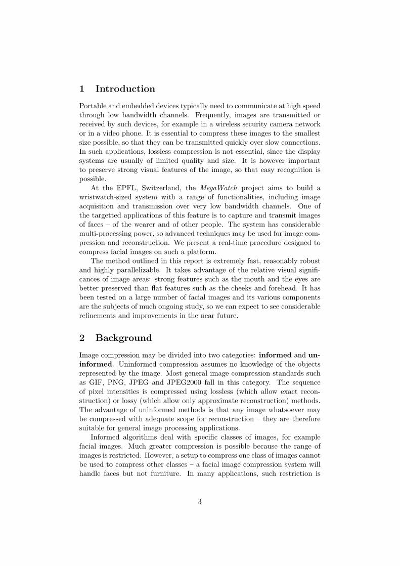
We observe that each of the errors above is a simple quadratic function of theappropriate coefficients. Unconstrained quadratic programming can be usedto minimize each error. Consider the texture error. It may be minimizedwith respect to the vector b as follows:

1. Transform the error formula: (For clarity, the [x, y] suffixes are notshown. Also, the vector {T1, T2, . . . Tn} is written as T.)

Etexture(b) =∑

x,y

(Tnovel − b.T

)2

=∑

x,y

(T 2

novel − 2Tnovelb.T + (b.T)2)

=∑

x,y T 2novel − 2

∑x,y Tnovelb.T +

∑x,y(b.T)2

=∑

x,y T 2novel − 2

∑x,y Tnovelb.T +

∑x,y b(TTT)bT

=∑

x,y T 2novel − b.(2

∑x,y TnovelT) + b(

∑x,y TTT)bT

The error is now in the standard form k + b.g + bHbT of a quadraticprogramming objective function, with g = −2

∑x,y TnovelT and H =∑

x,y TTT.

2. Compute the derivative of the error with respect to b:

d(k + b.g + bHbT )db

= gT + 2HbT

thereforedEtexture

db= −2

∑x,y

TnovelT +(2

∑x,y

TTT)bT

7

3. Set the derivative to zero. This defines an extremum of the errorfunction. Since our error is a non-negative quadratic function, thisextremum must be the minimum.

−2∑x,y

TnovelT +(2

∑x,y

TTT)bT = 0

or ( ∑x,y

TTT)bT =

∑x,y

TnovelT

Evaluating the matrices∑

x,y TTT and∑

x,y TnovelT is straightfor-ward.

4. Solve the above system for the best match coefficients b. We used LUdecomposition in our experiments.

3.3 Faster Matching: Orthonormal Bases and Projection

The approach of the last section is reasonably effective, but by precondi-tioning the sample set during model construction we can have much fastermatching. The trick is to transform the set of sample vectors into an or-thonormal basis. Adding up the projections of the novel vector onto theelements of the basis, we obtain the best match to the novel vector, mea-sured in terms of the sum of squared errors (which is nothing but the squaredL2 distance between the vectors). The following lemma proves this.

Lemma 1. Let V be an n-dimensional subspace of Rm, n < m. Let {Bi}be an orthonormal basis of V . Given a vector X ∈ Rm, the element of Vclosest to X is

n∑i=1

(X.Bi)Bi

where the “closest” element C is defined as that which minimizes the squaredL2 distance ‖X−C‖2.

Proof. Let C =∑n

i=1(X.Bi)Bi, and let ∆X = X − C. Consider the dotproduct of this vector with the elements of the basis.

∆X.Bj = (X−∑n

i=1(X.Bi)Bi).Bj

= X.Bj − (∑n

i=1(X.Bi)Bi).Bj

= X.Bj −∑n

i=1 δijX.Bi (since the basis is orthonormal)= X.Bj −X.Bj

= 0

(Here δij is the Kronecker delta: δij = 1 if i = j, 0 otherwise.)

8

So ∆X is orthogonal to any vector in V .

Now consider any vector C′ other than C in V . Since vector spaces areclosed under linear combination, C′ −C is in V . Let Y = C′ −C. Then,

‖X−C′‖2 = ‖X−C−Y‖2

= ‖∆X−Y‖2

= (∆X−Y).(∆X−Y)= ∆X.∆X + Y.Y − 2∆X.Y

But ∆X is orthogonal to Y, since Y ∈ V . Therefore 2∆X.Y = 0. So,

‖X−C′‖2 = ∆X.∆X + Y.Y= ‖∆X‖2 + ‖Y‖2

> ‖∆X‖2

= ‖X−C‖2

Therefore C =∑n

i=1(X.Bi)Bi is indeed the element of V “closest” toX.

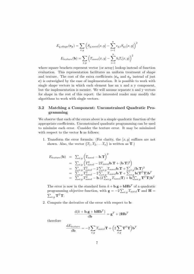
Each projection takes time linear in the size of the vectors. If eachvector has m dimensions (which is, in our case, the number of pixels ineach image), then the matching is performed in O(mn) time. Compare thiswith the equation-solving approach, which takes O(mn2 + n3) time (theusual algorithms for solving a system of n linear equations, such as LUdecomposition, contribute the O(n3) term). Actually, since n (number ofvectors) is always assumed to be less than m (dimensionality of vectors) inour application to maintain linear independence, the latter approach takesO(mn2) time in general.

In our experiments, projection gave matching times of the order of 100milliseconds, compared to 5 seconds for equation-solving. Section 5 givesmore details.

3.4 Principal Component Analysis and Eigenvectors

In practice, the transformation to an orthonormal basis is not performed onthe sample vectors themselves, but on the deviations of the sample vectorsfrom their mean. This complication is introduced by Principal Compo-nent Analysis (PCA), which has the benefit of reducing the size of thesample space by discarding “less significant” elements from the basis. PCAtransforms a set of linearly independent vectors {Xi, i = 1 . . . n} as follows:

1. Let X be the mean of the Xi’s.

9

2. Consider the set of vectors {X′i | X′

i = Xi − X}. This set has rankn− 1, since

n∑i=1

X′i =

n∑i=1

(Xi −X) =n∑

i=1

Xi − n

∑ni=1 Xi

n= 0

3. PCA gives an orthonormal basis {Ei} of size n − 1 for the spacespanned by the set {X′

i}. PCA additionally reduces the size of thebasis by discarding “less significant” elements, but we will ignore thisin our discussion for the moment. The Ei’s are conventionally calledeigenvectors.

After constructing the basis, we match a novel vector Xnovel as follows:

1. Compute X′novel = Xnovel −X

2. Project X′novel onto each eigenvector Ei, obtaining scalars ei = Ei.Xnovel.

Note that all eigenvectors are of unit length, since the basis is orthonor-mal.

3. Approximate Xnovel as X +∑n−1

i=1 eiEi.

We observe that∑n−1

i=1 eiEi is equivalent to∑n

i=1 kiX′i for some ki’s,

since the sets {Ei} and {X′i} span the same space. So our approximation

can be rewritten as

Xapprox = X +n∑

i=1

kiX′i

Lemma 2. The set of all possible approximations of the above form is{n∑

i=1

biXi,∑

bi = 1

}Proof.

Xapprox = X +∑n

i=1 kiX′i

=∑n

i=1 Xi

n +∑n

i=1 ki(Xi −∑n

j=1 Xj

n )

=∑n

i=1(ki + 1n −

∑nj=1 kj

n )Xj

=∑n

i=1 biXi

where bi = ki + 1n −

∑nj=1 kj

n = ki + 1n − k.

Now, ∑ni=1 bi =

∑ni=1(ki + 1

n −∑n

j=1 kj

n )

=∑n

i=1 ki + 1 + n∑n

j=1 kj

n=

∑ni=1 ki + 1−

∑nj=1 kj

= 1

10

We must show that each possible set of bi’s summing to 1 correspondsto some set of ki’s. Let us take any such set of bi’s. Then we can write:

b1 = k1 + 1n −

∑nj=1 kj

n

b2 = k2 + 1n −

∑nj=1 kj

n... =

...

bn = kn + 1n −

∑nj=1 kj

n

We must show that this system of equations is consistent, i.e. it has asolution for the ki’s. Let us construct a solution as follows:

Let∑n

j=1 kj = K, where K is any arbitrary real number. Solving for theki’s:

k1 = b1 − 1n + K

n

k2 = b2 − 1n + K

n... =

...kn = bn − 1

n + Kn

Adding all the equations and observing that K =∑n

j=1 kj , we get backour original condition

∑ni=1 bi = 1. Hence the system is consistent and the

solution is valid. We note that our choice of bi’s corresponds to an infinitenumber of possible choices for the ki’s, differing in the sum

∑nj=1 kj .

Theorem 1. Approximation by projection onto eigenvectors is equivalentto minimizing the L2 distance between a novel vector Xnovel and the vectorspace V1 = {

∑ni=1 biXi,

∑bi = 1}.

Proof. In the procedure outlined previously, we first construct X′novel =

Xnovel − X, then project X′novel onto each of the eigenvectors to obtain

coefficients, then take the linear combination of the eigenvectors weighted bythese coefficients, and finally add the mean X to obtain the approximation.So the approximation may be written as:

Xapprox = X +n−1∑i=1

(X′novel.Ei)Ei

We note, from Lemma 2, that the space of possible approximations isprecisely V1.

Let X′approx =

∑n−1i=1 (X′

novel.Ei)Ei. From Lemma 1, X′approx is the point

in the space V ′ spanned by {Ei} that minimises the L2 distance to X′novel.

Now, we observe that

11

Figure 3: Matches to the novel image (a) obtained by retaining b) all 49, c)30, d) 15 and e) 7 eigenvectors.

‖Xnovel −Xapprox‖2 = ‖Xnovel − (X + X′approx)‖2

= ‖(Xnovel −X)−X′approx‖2

= ‖X′novel −X′

approx‖2

So minimizing the L2 distance between X′novel and X′

approx correspondsto minimizing the L2 distance between Xnovel and Xapprox.

Also, there is a one-to-one correspondence between V1 and V ′:

X ∈ V ′ ↔ (X + X) ∈ V1

Hence the minimization is over the whole of V1.Therefore Xapprox, as constructed above, minimizes the L2 distance from

V1 to Xnovel.

We thus conclude that matching by projection onto the PCA space yieldsexactly the same best matches as quadratic programming, with the con-straint that the sum of the coefficients of the sample vectors must be 1. Inour experiments, we observed that except in cases where lighting conditions,shape or overall intensity deviated drastically from the images of the sampleset, this constraint was not very restrictive and the best matches from thetwo methods were virtually identical. Further, by retaining only the firstfew principal components, we reduced the number of projections required,thus speeding up the matching and generating excellent approximations tothe matches produced with the full eigenspace. Fig. 3 demonstrates this.

12

4 Feature-Based Optimizations

The eigenvector-projection approach is fast, but has a significant associatedchallenge: the separation of the novel image into shape and texture com-ponents must be done as accurately as possible. This calls for a robustalgorithm to set points in two facial images in correspondence.

The simplest approach is to compute the optical flow between the refer-ence image and the novel image – the flow field is taken as the correspondencefield. This approach is conceptually flawed, because optical flow algorithmsare designed to track points on the same object across multiple frames, notlocate corresponding points in images of different objects. However, sincetwo faces are superficially similar, this approach works reasonably well inpractice.

We experimented with the Bergen-Hingorani algorithm [1] for dense op-tical flow. It gave acceptable results on the whole, but spurious correspon-dences were frequently generated. Larger window sizes gave noticeably bet-ter results.

More sophisticated algorithms designed specifically for computing facialcorrespondences exist, but they are usually also more computation-intensiveand not suitable for real-time processing.

To develop a suitable algorithm for our application which gave few spu-rious correspondences and ran in real-time, we took note of the followingfacts:

• Certain points in facial images are easier to track than others. Findingcorrespondences for a point at the corner of the mouth where contrastand texture are strong is, for instance, easier than for a point in themiddle of the cheek, where the surface is smooth and unbroken.

• Correspondence fields between two facial images are smooth. Thisis to be expected since human faces have elastic, organic structure.This suggests that the field can be approximated fairly accurately byinterpolation from a set of “defining points”.

• Human vision is sensitive to strong features. When we observe a face,recognition is triggered more by the intensity variation in sharply-defined regions such as the overall outline, the eyes, the nose and themouth than in undistinguished ones such as the cheek and forehead.Therefore, in compressing a facial image, it is important to preserve thestructure of strong features using accurate correspondences at theselocations, but other regions need not be rendered so exactly.

A suitable correspondence algorithm could therefore select a set of easilytrackable feature points, compute correspondences at these points only, andinterpolate from the resulting values to obtain the correspondences at every

13

pixel in the source image. By not tracking weakly-defined points (whichresemble their neighbours), spurious correspondences may be reduced.

We implemented this method in the following manner:

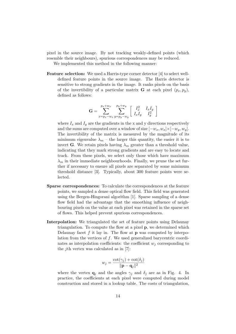
Feature selection: We used a Harris-type corner detector [4] to select well-defined feature points in the source image. The Harris detector issensitive to strong gradients in the image. It ranks pixels on the basisof the invertibility of a particular matrix G at each pixel (px, py),defined as follows:

G =px+wx∑

x=px−wx

py+wy∑y=py−wy

[I2x IxIy

IxIy I2y

]where Ix and Iy are the gradients in the x and y directions respectivelyand the sums are computed over a window of size [−wx, wx]×[−wy, wy].The invertibility of the matrix is measured by the magnitude of itsminimum eigenvalue λm – the larger this quantity, the easier it is toinvert G. We retain pixels having λm greater than a threshold value,indicating that they mark strong gradients and are easy to locate andtrack. From these pixels, we select only those which have maximumλm in their immediate neighbourhoods. Finally, we prune the set fur-ther if necessary to ensure all pixels are separated by some minimumthreshold distance [3]. Typically, about 300 feature points were se-lected.

Sparse correspondences: To calculate the correspondences at the featurepoints, we sampled a dense optical flow field. This field was generatedusing the Bergen-Hingorani algorithm [1]. Sparse sampling of a denseflow field had the advantage that the smoothing influence of neigh-bouring pixels on the value at each pixel was retained in the sparse setof flows. This helped prevent spurious correspondences.

Interpolation: We triangulated the set of feature points using Delaunaytriangulation. To compute the flow at a pixel p, we determined whichDelaunay facet f it lay in. The flow at p was computed by interpo-lation from the vertices of f . We used generalized barycentric coordi-nates as interpolation coefficients: the coefficient wj corresponding tothe jth vertex was calculated as in [7]:

wj =cot(γj) + cot(δj)

‖p− qj‖2

where the vertex qj and the angles γj and δj are as in Fig. 4. Inpractice, the coefficients at each pixel were computed during modelconstruction and stored in a lookup table. The costs of triangulation,

14

Figure 4: Barycentric coordinates in an irregular convex polygon.

point location and barycentric coordinate computation were thereforenot incurred during matching. We developed this approach from origi-nal ideas, but discovered later that Kardouchi et al [6] had done similarwork.

Fig. 5 illustrates the entire process.

4.1 Features for Speed

Although our feature-based approach was initially designed to generate goodcorrespondences, we observed that it could also be used to drastically speedup the matching process. The shape components were completely definedby their values at the feature points. Hence, we could restrict the shapevectors to these values only, reducing their dimensionality from m, the totalnumber of pixels in each image, to nf , the number of feature points. In ourexperiments with 256 × 256 images and 300 feature points, this implied areduction from 65536 dimensions to 300.

We compute the PCA space of the restricted shape vectors and matchby projection onto this space. The projection-based approach executes in

Figure 5: The feature-based interpolation process. For clarity, backgroundtriangles are not shown in the Delaunay triangulation. The interpolationmap is colour-coded: each feature point is assigned an unique intensity andthe intensity at each pixel is obtained by interpolation from the appropriatefeature points.

15

time linear in the dimensionality of the vectors, so execution time is reducedfrom O(mn) (see Section 3.3) to O(nfn). The full (dense) shape compo-nent is approximated after matching, by interpolating from the best matchrestricted shape.

Ideally, we would like to show that matching with restricted vectors firstand interpolating afterwards is equivalent to interpolating first and matchingwith full vectors afterwards.

4.1.1 Investigating Equivalence

We are given a set X of n linearly independent vectors {Xi, i = 1 . . . n}in Rm, n < m. We are also given a set Y of “restricted vectors” {Yi, i =1 . . . n} in Rnf , nf < m. These sets have the following property: for any j:

X1j =∑nf

k=1 cjkY1k

X2j =∑nf

k=1 cjkY2k... =

...Xnj =

∑nf

k=1 cjkYnk

where Xij denotes the jth element of Xi and Yij denotes the jth element ofYi. The cjk’s are a set of scalar interpolation coefficients – there is one suchset for each j. In simple terms, the set X may be obtained by interpolationfrom the set Y .

We are now given a novel vector Xnovel ∈ Rm and the correspondingrestricted vector Ynovel ∈ Rnf , related by the same sets of interpolationcoefficients as above: for any j:

Xnovel,j =nf∑

k=1

cjkYnovel,k

We obtain two approximations to Xnovel as follows:

1. Minimize the L2 distance from the space spanned by the elements ofX to Xnovel, obtaining the closest match X1

approx.

2. Minimize the L2 distance from the space spanned by the elements of Yto Ynovel, obtaining the closest match Yapprox. Now interpolate fromYapprox using the coefficients {cjk} to obtain X2

approx.

We ask if and under what conditions X1approx and X2

approx are equal.We are currently working on an answer to this question.

4.1.2 Theoretical Speed Gain

We conclude this section with some explicit calculations for the speed gainfrom the feature-based approach, compared to the case when full vectors are

16

projected for all components. We assume that features are used to restrictonly the two shape components (x and y), not the texture component. Wealso assume that the platform is serial-processing, not parallel-processing.

As mentioned previously, each shape component restricted to the featurepoints is projected onto the set of eigenvectors in O(nfn) time, comparedto O(mn) for projecting full vectors. This results in a net speed gain by afactor of g:

g =3×O(mn)

O(mn) + 2×O(nfn)

If a sequence of one multiplication and one addition (a unit operation inprojection) takes time τ , then the speed gain is:

g =3mnτ

mnτ + 2nfnτ=

3m

m + 2nf= 3−

6nf

m + 2nf

For practical purposes, nf � m, so g ≈ 3: we expect the feature-basedapproach to be three times faster in projection. (Matching in PCA spacerequires us to add the mean, but this is linear in the dimensions of thevectors and does not change g.) The results satisfy our expectations: asnoted in Section 5, feature-based projection takes ∼20ms while full-vectorprojection takes ∼60ms. We exclude the (more or less identical) times takento compute correspondences in the two approaches.

If the texture vectors could somehow be restricted as well, i.e. if wecould predict an entire texture map from values at feature points, then thespeedup is g = m/nf , typically of the order of a few hundred.

5 Implementation and Results

We implemented our approach on a dual 2.7 GHz Pentium 4 system with1GB RAM, running RedHat Linux 9 (Shrike) with the symmetric multi-processing (SMP) kernel 2.4.20-8smp. A uname -a command yielded thefollowing:

Linux lappc16.epfl.ch 2.4.20-8smp #1 SMP Thu Mar 13 17:45:54 EST2003 i686 i686 i386 GNU/Linux

The coding language was C. OpenCV-0.9.5 was used as the image-processing library. No explicit multi-processing or threading instructionswere included in the source code.

In our experiments, we obtained a minimum average matching time of120ms. A slightly slower implementation which was easier to time took140ms, of which 120ms was for computing sparse correspondences (pruninga Bergen-Hingorani optical flow field) and 20ms for projecting feature-based

17

restricted vectors. We quote the times from the latter implementation sincewe are more confident that the timing was accurate.

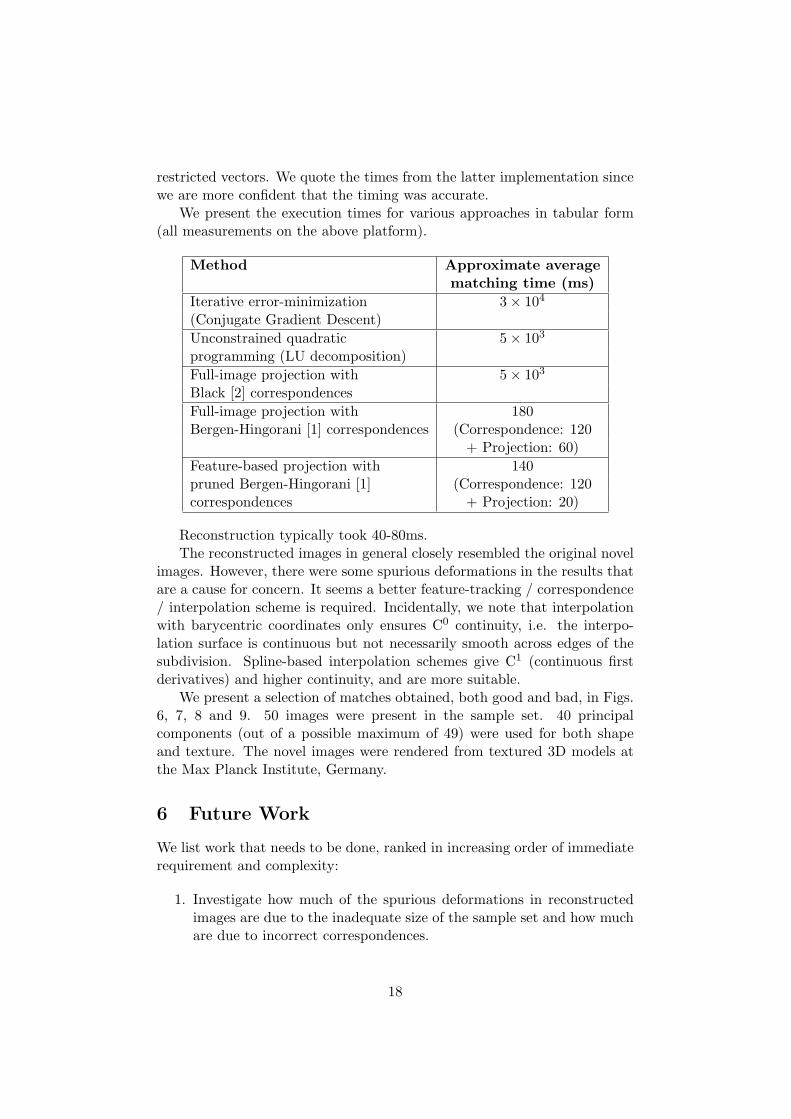
We present the execution times for various approaches in tabular form(all measurements on the above platform).

Method Approximate averagematching time (ms)

Iterative error-minimization 3× 104

(Conjugate Gradient Descent)Unconstrained quadratic 5× 103

programming (LU decomposition)Full-image projection with 5× 103

Black [2] correspondencesFull-image projection with 180Bergen-Hingorani [1] correspondences (Correspondence: 120

+ Projection: 60)Feature-based projection with 140pruned Bergen-Hingorani [1] (Correspondence: 120correspondences + Projection: 20)

Reconstruction typically took 40-80ms.The reconstructed images in general closely resembled the original novel

images. However, there were some spurious deformations in the results thatare a cause for concern. It seems a better feature-tracking / correspondence/ interpolation scheme is required. Incidentally, we note that interpolationwith barycentric coordinates only ensures C0 continuity, i.e. the interpo-lation surface is continuous but not necessarily smooth across edges of thesubdivision. Spline-based interpolation schemes give C1 (continuous firstderivatives) and higher continuity, and are more suitable.

We present a selection of matches obtained, both good and bad, in Figs.6, 7, 8 and 9. 50 images were present in the sample set. 40 principalcomponents (out of a possible maximum of 49) were used for both shapeand texture. The novel images were rendered from textured 3D models atthe Max Planck Institute, Germany.

6 Future Work

We list work that needs to be done, ranked in increasing order of immediaterequirement and complexity:

1. Investigate how much of the spurious deformations in reconstructedimages are due to the inadequate size of the sample set and how muchare due to incorrect correspondences.

18

Figure 6: A selection of novel images (first and third columns) and thecorresponding feature-based matches (second and fourth columns): somegood, some not-so-good. Part 1.

19

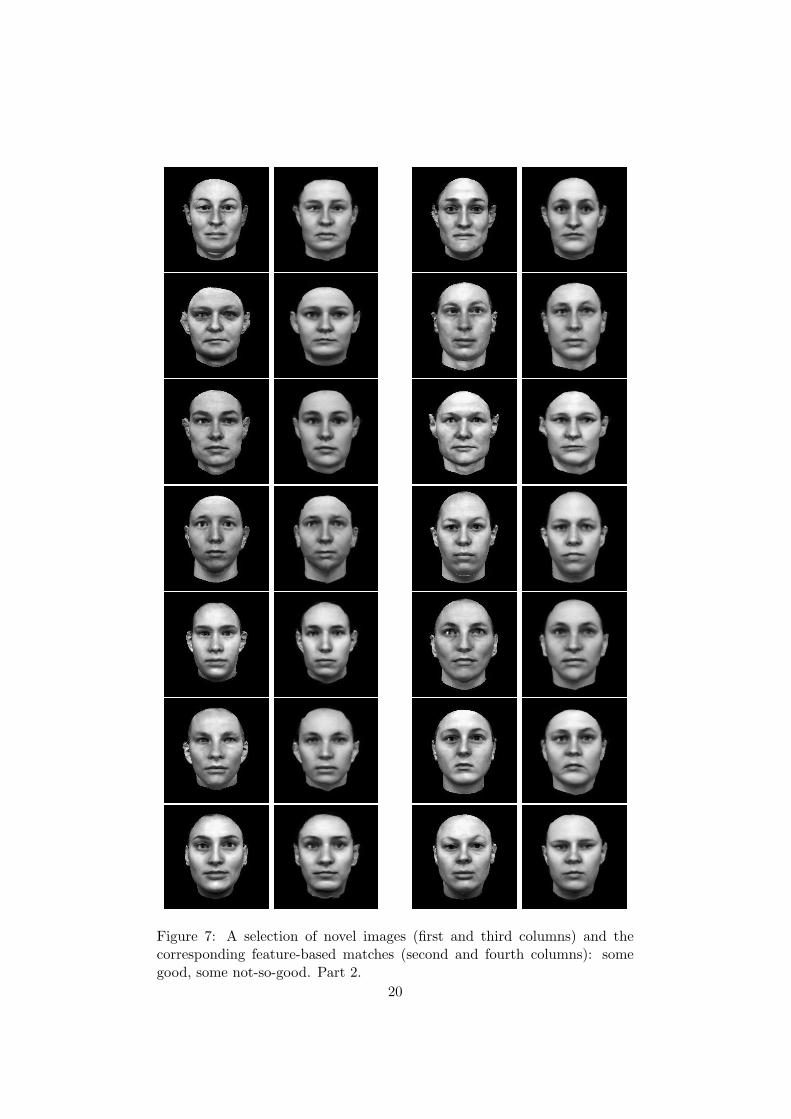
Figure 7: A selection of novel images (first and third columns) and thecorresponding feature-based matches (second and fourth columns): somegood, some not-so-good. Part 2.

20

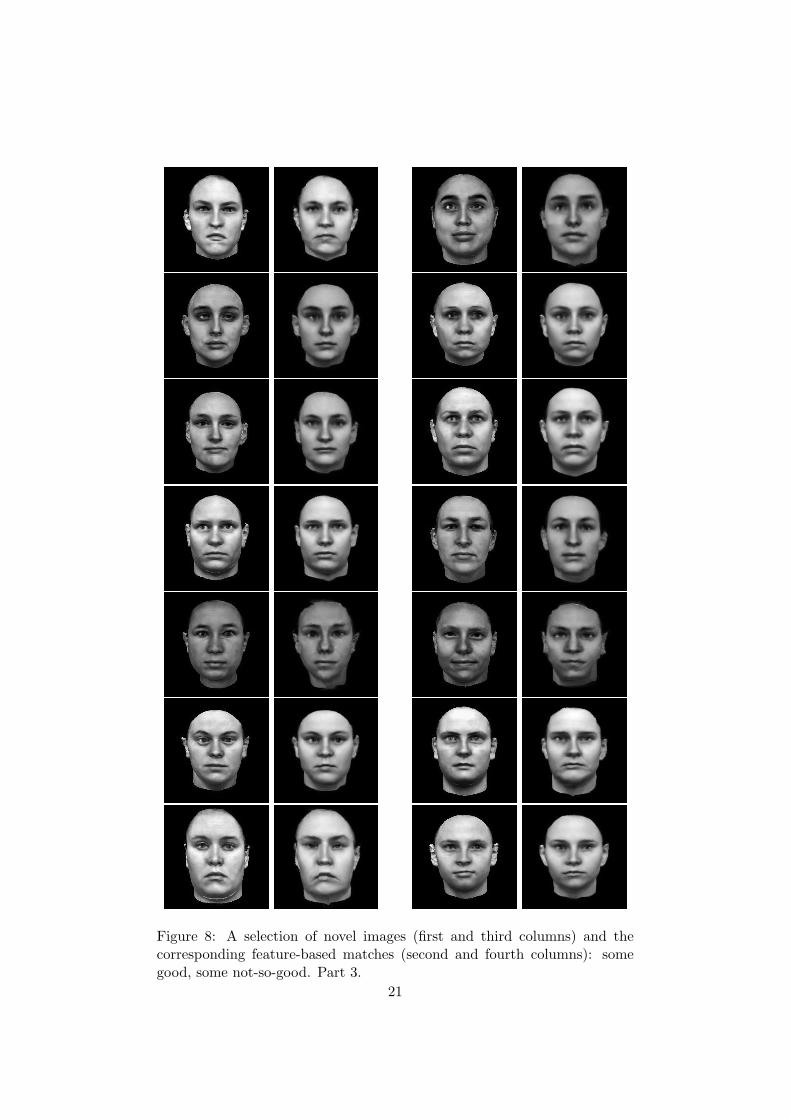
Figure 8: A selection of novel images (first and third columns) and thecorresponding feature-based matches (second and fourth columns): somegood, some not-so-good. Part 3.

21

Figure 9: A selection of novel images (first and third columns) and thecorresponding feature-based matches (second and fourth columns): somegood, some not-so-good. Part 4.

22

2. Obtain substantial quantitative information about the performance ofthe algorithm. Measure running times on a variety of facial images,and also measure the accuracy of the approximation using multiplenorms.

3. Implement a smoother interpolation scheme, such as a spline-basedapproach.

4. Implement the algorithm on a parallel-processing platform. The al-gorithm is highly parallelizable and a large speed increase could beachieved in a multi-processor environment.

5. Investigate whether preprocessing by wavelet decomposition and sim-ilar techniques can give smaller and more workable images to increaseaccuracy and speed.

6. Research, develop and implement a method to extend the feature-based approach to texture components as well. This will make projec-tion a few hundred times more efficient.

7. Research, develop and implement a better correspondence scheme.The performance of the algorithm really hinges on just this step.

Acknowledgements

I am grateful to Dr. Edoardo Charbon and Randhir K. Singh of the EPFL,Switzerland, for their suggestions, encouragement and patience. Randhirwrote the code for matching morphable models by error-minimization whichformed the basis for my efforts, and provided help and advice at crucialstages. He is also responsible for the idea of using wavelet decompositionsfor better matching, a work-in-progress. I also thank the people at theProcessor Architecture Laboratory, EPFL, who tolerated me for two-and-a-half months, and the countless people in the scientific community whoseideas and publications influenced my work.

References

[1] J. Bergen and R. Hingorani, “Hierarchical Motion-Based Frame RateConversion,” Technical Report, David Sarnoff Research Center, Prince-ton, 1990.

[2] M. J. Black, “Robust Incremental Optical Flow,” Ph.D. Thesis, Yale,1992.

23

[3] J.-Y. Bouget, “Pyramidal Implementation of the Lucas Kanade Fea-ture Tracker: Description of the Algorithm,”, Microprocessor ResearchLabs, Intel Corp., 2000.

[4] C. Harris and M. Stephens, “A combined corner and edge detector,”Proc. Alvey Vision Conf., pp.147-151, 1988.

[5] M. J. Jones and T. Poggio, “Model-Based Matching by Linear Combi-nations of Prototypes,” unpublished AI memo, MIT, 1996.

[6] M. Kardouchi, J. Konrad and C. Vazquez, “Estimation of large-amplitude motion and disparity fields: Application to intermediate viewreconstruction,” Proc. Visual Communications and Image Processing,IS&T/SPIE Symp. on Elec. Imaging, San Jose, 2000.

[7] M. Meyer, Haeyoung L., A. Barr, M. Desbrun, “Generalized Barycen-tric Coordinates on Irregular Polygons,”, Journal of Graphics Tools,7(1):pp.13-22, 2002.

[8] T. Vetter and N. F. Troje, “Separation of texture and shape in imagesof faces for image coding and synthesis,” JOSA, A 14:9 pp.2152-2161,1997.

24