More than just a game:What quantitative study of sports can teach us

about general principles of statistics

Andrew GelmanDepartment of Statistics and Department of Political Science

Columbia University, New York

7 Mar 2016

Classic statistics problems in sports

I In-game decisionsI Swing at the first pitch?I Go for it on 4th down?

I Player evaluationI Predict season outcome from aggregated individual statisticsI Predictions and adjustments (age, context, . . . )

I Predictions and odds

I . . .

Some things Bill James taught us

I Outs matterI On-base averageI Caught stealing

I At what age are players at their peak?

I Beware statistical illusions

I Minor league stats predict major-league performance

I . . .

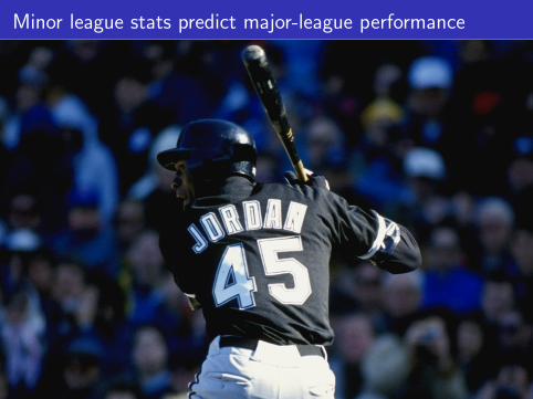
Minor league stats predict major-league performance

A friend from Alaska writes:

“Palin’s magic formula for success has been simply been to ignorepartisan crap and get down to the boring business of fixing up abroken government . . . The real significance of Gov Palin’s successand her phenomenal approval ratings is that they demonstrate hergenuine talent as a non-partisan.”

Do minor league stats predict major-league performance?

My Alaskan friend continues:

“Sarah Palin is not just popular. She is fantastically popular. Herpercentage approval ratings have reached the 90s. Even now, witha minor nepotism scandal going on, she’s still about 80%. . . . Howdoes one do that? You might get 60% or 70% who are rabidlyenthusiastic in their love and support, but youre also going to get asolid core of opposition who hate you with nearly as much passion.The way you get to 90% is by being boringly competent whileremaining inoffensive to people all across the political spectrum.”

Popularity of governors

Popular governor, small state

Governor popularity, state size, and the economy

We fit a linear regression (n = 50):

lm (popularity ~ c.log.statepop + c.income.change)

coef.est coef.se

(Intercept) 48.6 2.2

c.log.statepop -6.1 2.3

c.income.change 2.4 1.7

How is baseball different from politics?

I One goal (winning) vs. two (winning and policy)I Ability vs. being in right place at right downI Single vs. different environmentsI Different individual career optionsI Small N vs. large N

But even the Master is not perfect

“Are athletes special people? In general, no, but occasionally, yes.Johnny Pesky at 75 was trim, youthful, optimistic, and practicallyexploding with energy. You rarely meet anybody like that who isn’tan ex-athlete—and that makes athletes seem special.”— Bill James, 2001.

I Do the math:

Pr(athlete | 75 and energetic) ∝ Pr(athlete) Pr(75 and energetic | athlete)

Rating soccer teams

The model in Stan

parameters {

real b;

real<lower=0> sigma_a;

real<lower=0> sigma_y;

vector[nteams] eta_a;

}

transformed parameters {

vector[nteams] a;

a <- b*prior_score + sigma_a*eta_a;

}

model {

eta_a ~ normal(0,1);

for (i in 1:ngames)

sqrt_dif[i] ~ student_t(df, a[team1[i]]-a[team2[i]],sigma_y);

}

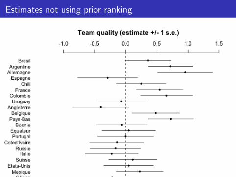
Estimates not using prior ranking

Lessons from World Cup example

I Model score differential, not simple wins and losses—even ifyour only goal is to predict wins and losses

I Same thing in education (model test scores rather thanpass/fail) and elections (model vote share not win/loss)

I Jump in and fit a model, then check its fit to data

I Combine sources of information

I Compare different fits graphically

Does it hurt to have a team full of superstars?

The research paper

The curve they fit to the data

What ordinary people expected to see

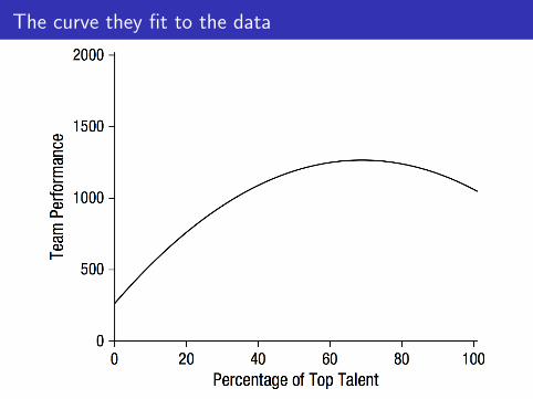
The curve they fit to the data

The range of the data

The curve they fit to the data . . .

. . . the data!

Lessons from superstars example

I Plot data and model together

I Don’t overinterpret statistical significance

I Be careful with nonlinear models

Halftime motivation in basketball

I Economists Jonah Berger and Devin Pope:“Analysis of over 6,000 collegiate basketball games illustratesthat being slightly behind increases a team’s chance ofwinning. Teams behind by a point at halftime, for example,actually win more often than teams ahead by one. Thisincrease is between 5.5 and 7.7 percentage points . . . ”

I But . . . in their data, teams that were behind at halftime by 1point won 51.3% of the time

I Approx 600 such games; thus, std. error is 0.5/√

600 = 0.02

I Estimate ±1 se is [0.513± 0.02] = [0.49, 0.53]

I So where did they get “5.5 and 7.7 percentage points”??

Halftime motivation in basketball: the data and the fitted5th-degree polynomial

The data without the 5th-degree polynomial

“Robustness checks”

I Recent study: “a win in the 10 days before Election Daycauses the incumbent to receive an additional 1.61 percentagepoints of the vote in Senate, gubernatorial, and presidentialelections”

I County-level vote analysis

“Will Ohio States football team decide who wins theWhite House?”

“The key to victory could come down to . . . Florida, Ohio, andVirginia. On Oct. 27th, a little more than a week before theelection, the Ohio State Buckeyes have a big football game againstPenn State. The University of Florida Gators have a huge matchup against the University of Georgia Bulldogs. If the electionremains razor close, these games in these two key battlegroundstates could affect who sits in the White House for the next fouryears. Can you imagine Ohio State head coach Urban Meyergetting a late night call from the Obama campaign suggesting aparticular blitz package? Or maybe Romney has some advice forhow the Gators can bottle up Georgia’s running game. Thedecision of whether to punt or go for it on that crucial fourth downcould affect the job prospects of more than just the football teamscoaching staff.” — Tyler Cowen and Kevin Grier, Slate.com

Understanding the college football and elections study

I Assume that a win in the two weeks before the election givesthe incumbent an extra 2% of the vote

I What does this imply about the election?I Not so much . . .

I Diffusion: A shift of ±1% of the vote in the county containingColumbus, Ohio, corresponds to a 0.1% shift in the state

I Averaging: In the two weeks before the 2012 election, therewere 4 major-college football games involving Ohio teams, andmany more in Florida, Virginia, Colorado, etc.

Applying the statistical significance filter

I Results that are statistically significant are likely to beoverestimates

I Downgrade the estimated 2% effect

Lessons from football and elections example

I Map parameter estimates to the real world

I Published estimates are biased upward

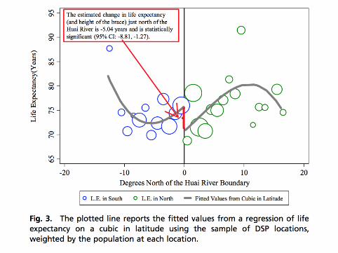
Same issues arise in policy analysis

●

●

●

●

●●

●

●●

●

●●

●

●

●

●●

●

●

0 5 10 15 20

0.0

0.2

0.4

0.6

0.8

1.0

Data on putts in pro golf

Distance from hole (feet)

Pro

babi

lity

of s

ucce

ss

1346/1443

577/694

337/455

208/353

149/272136/256

111/240

69/21767/200

75/237

52/20246/192

54/174

28/167

27/20131/195

33/19120/147

24/152

●

●

●

●

●●

●

●●

●

●●

●

●

●

●●

●

●

0 5 10 15 20

0.0

0.2

0.4

0.6

0.8

1.0

What's the probability of making a golf putt?

Distance from hole (feet)

Pro

babi

lity

of s

ucce

ss

Logistic regression, a = 2.2, b = −0.3

Geometry-based model

x

Rr

−2σ 0 2σ

Stan code

data {

int J;

int n[J];

real x[J];

int y[J];

real r;

real R;

}

parameters {

real<lower=0> sigma;

}

model {

real p[J];

for (j in 1:J)

p[j] <- 2*Phi(asin((R-r)/x[j]) / sigma) - 1;

y ~ binomial(n, p);

}

●

●

●

●

●●

●

●●

●

●●

●

●

●

●●

●

●

0 5 10 15 20

0.0

0.2

0.4

0.6

0.8

1.0

What's the probability of making a golf putt?

Distance from hole (feet)

Pro

babi

lity

of s

ucce

ss

Geometry−based model, sigma = 1.5

●

●

●

●

●●

●

●●

●

●●

●

●

●

●●

●

●

0 5 10 15 20

0.0

0.2

0.4

0.6

0.8

1.0

Two models fit to the golf putting data

Distance from hole (feet)

Pro

babi

lity

of s

ucce

ss

Logistic regression, a = 2.2, b = −0.3

Geometry−based model, sigma = 1.5

Lessons from golf example

I You can (sometimes) fit and interpret a theory-based model

I Plot data and model together

I Compare different fits graphically

Summary

I God is in every leaf of every treeI Statistics in sports:

I Variation, uncertainty, regularity, decision making . . . life!

I Science in sports:I Physiology, motivation, competition . . . life!