Mean Field Theory Solution of the Ising Model

Franz Utermohlen

September 12, 2018

Contents

1 Ising model 1

2 Mean field theory solution of the Ising model 22.1 Decoupling the Hamiltonian . . . . . . . . . . . . . . . . . . . . . . . . . . . 32.2 Self-consistency equation . . . . . . . . . . . . . . . . . . . . . . . . . . . . . 52.3 Critical behavior at zero field . . . . . . . . . . . . . . . . . . . . . . . . . . 7

2.3.1 Magnetization . . . . . . . . . . . . . . . . . . . . . . . . . . . . . . . 92.3.2 Susceptibility . . . . . . . . . . . . . . . . . . . . . . . . . . . . . . . 10

2.4 Free energy . . . . . . . . . . . . . . . . . . . . . . . . . . . . . . . . . . . . 11

3 Mean field theory solution of the Ising model with single-ion anisotropy 153.1 Decoupling the Hamiltonian . . . . . . . . . . . . . . . . . . . . . . . . . . . 153.2 Self-consistency equation . . . . . . . . . . . . . . . . . . . . . . . . . . . . . 16

1 Ising model

The (ferromagnetic) Ising model is a simple model of ferromagnetism that provides someinsight into how phase transitions and the non-analytic behavior of thermodynamic quantitiesacross phase transitions occur in physics. Consider a lattice containing a spin at each site thatcan point either up (+1) or down (−1). The (classical) nearest-neighbor Ising Hamiltonianfor this system is

H = −J∑〈ij〉

sisj − hN∑i=1

si , (1)

where J is a positive (ferromagnetic) coupling constant, 〈ij〉 denotes summation over nearestneighbors,1 si (= +1 or −1) is the value of the spin on the ith site, h is an external magneticfield pointing along the z direction,2 and N is the number of sites on the lattice.

1Each pair of sites is only included once in the sum.2h > 0 corresponds to the field pointing in the +z direction.

1

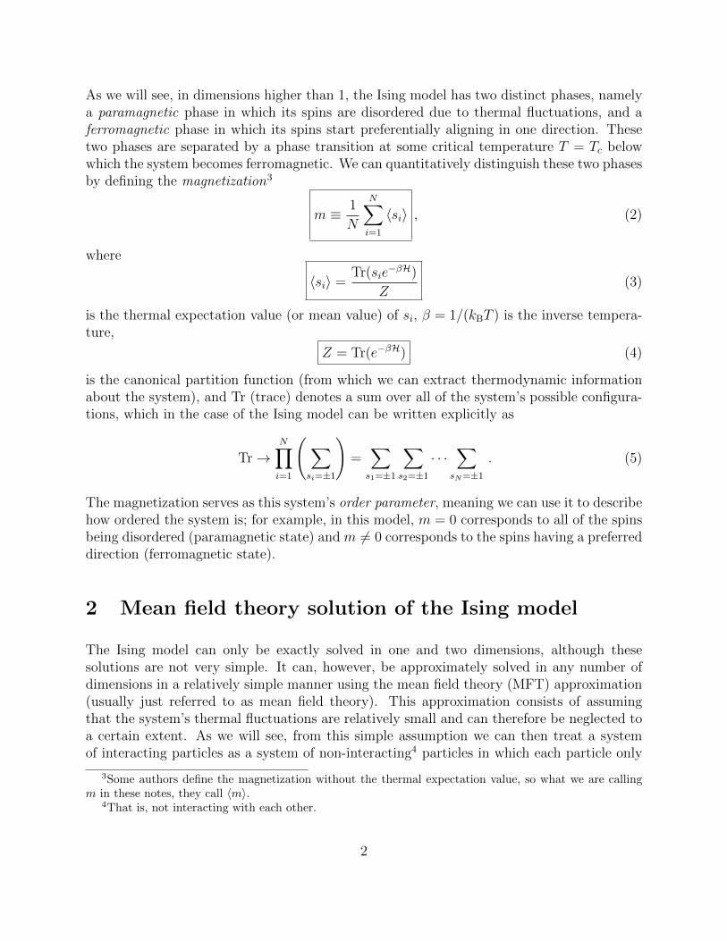
As we will see, in dimensions higher than 1, the Ising model has two distinct phases, namelya paramagnetic phase in which its spins are disordered due to thermal fluctuations, and aferromagnetic phase in which its spins start preferentially aligning in one direction. Thesetwo phases are separated by a phase transition at some critical temperature T = Tc belowwhich the system becomes ferromagnetic. We can quantitatively distinguish these two phasesby defining the magnetization3

m ≡ 1

N

N∑i=1

〈si〉 , (2)

where

〈si〉 =Tr(sie

−βH)

Z(3)

is the thermal expectation value (or mean value) of si, β = 1/(kBT ) is the inverse tempera-ture,

Z = Tr(e−βH) (4)

is the canonical partition function (from which we can extract thermodynamic informationabout the system), and Tr (trace) denotes a sum over all of the system’s possible configura-tions, which in the case of the Ising model can be written explicitly as

Tr→N∏i=1

(∑si=±1

)=∑s1=±1

∑s2=±1

· · ·∑sN=±1

. (5)

The magnetization serves as this system’s order parameter, meaning we can use it to describehow ordered the system is; for example, in this model, m = 0 corresponds to all of the spinsbeing disordered (paramagnetic state) and m 6= 0 corresponds to the spins having a preferreddirection (ferromagnetic state).

2 Mean field theory solution of the Ising model

The Ising model can only be exactly solved in one and two dimensions, although thesesolutions are not very simple. It can, however, be approximately solved in any number ofdimensions in a relatively simple manner using the mean field theory (MFT) approximation(usually just referred to as mean field theory). This approximation consists of assumingthat the system’s thermal fluctuations are relatively small and can therefore be neglected toa certain extent. As we will see, from this simple assumption we can then treat a systemof interacting particles as a system of non-interacting4 particles in which each particle only

3Some authors define the magnetization without the thermal expectation value, so what we are callingm in these notes, they call 〈m〉.

4That is, not interacting with each other.

2

interacts with a “mean field” that captures the average behavior of the particles aroundit. In other words, MFT effectively decouples the Hamiltonian into a simpler Hamiltoniandescribing a non-interacting system. This makes it a very powerful method that is used oftenin physics to explore the behavior of complicated many-body systems that cannot be solvedexactly.

Remarkably, even though the predictions MFT makes are quantitatively incorrect, it cor-rectly predicts the Ising model’s qualitative behavior for two dimensions and higher. This isbecause fluctuations are more important in lower dimensions, so the MFT approximation isless accurate in lower dimensions.

2.1 Decoupling the Hamiltonian

In order to decouple the Ising Hamiltonian using MFT, we start by writing each spin in thespin interaction terms sisj in the form

si = 〈si〉+ δsi , (6)

whereδsi ≡ si − 〈si〉 (7)

denotes fluctuations about the mean value of si. The spin interaction terms sisj thus be-come

sisj = (〈si〉+ δsi)(〈sj〉+ δsj)

= 〈si〉 〈sj〉+ 〈sj〉 δsi + 〈si〉 δsj + δsiδsj . (8)

We now make the assumption that the fluctuations are very small, so we can ignore the termquadratic in fluctuations:

δsiδsj = 0 . (9)

This is the approximation that MFT relies on: assuming fluctuations are small. The quantitysisj is then approximately

sisj ≈ 〈si〉 〈sj〉+ 〈sj〉 δsi + 〈si〉 δsj= 〈si〉 〈sj〉+ 〈sj〉 (si − 〈si〉) + 〈si〉 (sj − 〈sj〉)= 〈sj〉 si + 〈si〉 sj − 〈si〉 〈sj〉 . (10)

Since this system is translationally invariant, the expectation value 〈si〉 of any given site iis independent of the site, so we have

〈si〉 = m. (11)

We can then further simplify sisj to

sisj = m(si + sj)−m2 = m[(si + sj)−m] (12)

3

and approximate the Ising Hamiltonian as

HMF = −Jm∑〈ij〉

(si + sj −m)− hN∑i=1

si , (13)

where the subscript on the Hamiltonian reminds us that this is only an approximation ofthe Ising Hamiltonian. Since ∑

〈ij〉

si =∑〈ij〉

sj (14)

due to the symmetry of i and j in the sum over nearest neighbors, we can write∑〈ij〉

(si + sj) =∑〈ij〉

2si , (15)

so the Hamiltonian reads

HMF = −Jm∑〈ij〉

(2si −m)− hN∑i=1

si . (16)

We can write the sum over nearest neighbors as∑〈ij〉

→ 1

2

N∑i=1

∑j∈nn(i)

, (17)

where the factor of 1/2 is to avoid double counting pairs of sites and nn(i) denotes nearestneighbors of i. Since there is no explicit j dependence inside the summation, this inner sumis simply ∑

j∈nn(i)

= q , (18)

where the coordination number q is equal to the number of neighbors of any given site.5 Wethen have ∑

〈ij〉

→ q

2

N∑i=1

, (19)

so the Ising Hamiltonian further simplifies to

HMF = −qJm2

N∑i=1

(2si −m)− hN∑i=1

si

=NqJm2

2− qJm

N∑i=1

si − hN∑i=1

si

=NqJm2

2− (h+ qJm)

N∑i=1

si , (20)

5For example, for a 1D lattice, q = 2; for a 2D triangular lattice, q = 3; for a 2D square lattice, q = 4;etc.

4

or simply

HMF =NqJm2

2− heff

N∑i=1

si , (21)

whereheff ≡ h+ qJm (22)

is the effective magnetic field felt by the spins. We have now effectively decoupled theHamiltonian into a sum of one-body terms. Again, this conceptually means that particlesno longer interact with each other in this approximation, but rather interact only with aneffective magnetic field heff that is comprised of the external field h and the mean field qJminduced by neighboring particles.

2.2 Self-consistency equation

Let’s calculate the partition function using the mean field Ising Hamiltonian:

ZMF = Tr(e−βHMF)

=N∏i=1

(∑si=±1

)e−βHMF

=N∏i=1

(∑si=±1

)e−βNqJm

2/2eβheff∑N

j=1 sj

= e−βNqJm2/2

N∏i=1

(∑si=±1

eβheffsi

)

= e−βNqJm2/2

N∏i=1

(eβheff + e−βheff)︸ ︷︷ ︸=2 cosh(βheff)

= e−βNqJm2/2[2 cosh(βheff)]N , (23)

so we find

ZMF = e−βNqJm2/2[2 cosh(βheff)]N . (24)

Now, recall from Eq. 2 that the magnetization is given by

m ≡ 1

N

N∑i=1

〈si〉 .

5

Using Eq. 3, we can rewrite this as

m =1

N

N∑i=1

Tr(sie−βHMF)

ZMF

=1

N

1

ZMF

N∑i=1

sie−βHMF

=1

Nβ

1

ZMF

∂ZMF

∂heff

=1

Nβ

∂(lnZMF)

∂heff

, (25)

where on the third line we have used the fact that

∂ZMF

∂heff

=∂

∂heff

Tr(e−βHMF)

= Tr

(∂

∂heff

e−βHMF

)= −β Tr

(∂HMF

∂heff

e−βHMF

)= −β Tr

[(−

N∑i=1

si

)e−βHMF

]

= β Tr

[N∑i=1

sie−βHMF

]. (26)

Now, from Eq. 24 we can calculate lnZMF:

lnZMF = −βNqJm2

2+N ln 2 +N ln[cosh(βheff)] , (27)

so∂(lnZMF)

∂heff

= Nβ tanh(βheff) . (28)

Inserting this back into Eq. 25 gives

m = tanh(βheff) . (29)

Inserting the definition of heff (Eq. 22) back into this equation gives us the self-consistencyequation

m = tanh[β(h+ qJm)] . (30)

This is a transcendental equation, so we cannot solve for m analytically. However, we cansolve for m graphically by plotting m and tanh[β(h+ qJm)] (for fixed values of β, h, q, andJ).

6

Let’s consider the special case of h = 0. In Figure 1 we plot m and tanh(βqJm) on the sameplot for various values of βqJ . We can graphically see that the solutions are qualitativelydifferent when βqJ ≤ 1 and βqJ > 1.6 These two cases can be understood as follows:

• βqJ ≤ 1 (i.e., kBT ≥ qJ): There is only one solution: m = 0. This corresponds to thesystem being in a paramagnetic state.

• βqJ > 1 (i.e., kBT < qJ): There are three solutions: m = 0 and m = ±m0, wherem0 ≤ 1. The m = ±m0 solutions correspond to the system being in a ferromagneticstate (the system is magnetized). As we will discuss later, the m = 0 solution turnsout to be unstable, so we physically only observe either m = m0 or m = −m0 at thesetemperatures.

The critical temperature Tc below which the system becomes spontaneously magnetizedwithout any external magnetic fields is therefore given by

kBTc = qJ . (31)

It should be noted that for the 1D case, MFT thus predicts a magnetic phase transitionat kBTc = 2J ; however, solving this system exactly we find that there is in fact no phasetransition in 1D. Thermal fluctuations turn out to be strong enough to destroy the system’smagnetic ordering in 1D, so MFT provides a qualitatively incorrect result in this specificcase.

As mentioned earlier, MFT is more accurate in higher dimensions. For example, for the 2Dsquare lattice, MFT predicts kBTc = 4J , whereas solving the system exactly we find thatkBTc = 2J/ ln(1 +

√2) ≈ 2.27J . Also note that since MFT assumes fluctuations are small,

it generally overestimates the system’s tendency to order and thus overestimates the valueof Tc.

2.3 Critical behavior at zero field

In this section we discuss the behavior of the system near the critical temperature Tc. Inorder to more easily look at the behavior for T → Tc, let’s define the reduced temperature t

6We can also reach this conclusion a bit more rigorously by noting that there are three solutions when[d

dmtanh(βqJm)

]∣∣∣∣m=0

> 1 ,

and one solution otherwise. Evaluating the derivative gives[d

dmtanh(βqJm)

]∣∣∣∣m=0

=

[βqJ

1

cosh2(βqJm)

]∣∣∣∣m=0

= βqJ ,

so we find that we have three solutions solution when βqJ > 1, and one solution otherwise.

7

-1.0 -0.5 0.5 1.0m

-1.0

-0.5

0.5

1.0

βqJ = 0.5

m

tanh(0.5m)

-1.0 -0.5 0.5 1.0m

-1.0

-0.5

0.5

1.0

βqJ = 1

m

tanh(m)

-1.0 -0.5 0.5 1.0m

-1.0

-0.5

0.5

1.0

βqJ = 1.5

m

tanh(1.5m)

Figure 1: Solving the self-consistent equation graphically for h = 0 and various values of βqJ .The top plot is at T > Tc, the middle plot is at T = Tc, and the bottom plot is at T < Tc.

8

by

t ≡ T − TcTc

. (32)

We can then look at the critical behavior by expanding around small t.

2.3.1 Magnetization

We already know that when there is no external magnetic field, we have m = 0 when T ≥ Tc.Let’s explore further what happens in the critical regime just below Tc (i.e., T → T−c ) atzero field (h = 0). Using the expansion

tanh(x) = x− x3

3+O(x5) (33)

around x = 0, we can rewrite the self-consistency equation (Eq. 30) for h = 0 around m = 0(near Tc) as

m = βqJm− 1

3(βqJm)3

=

(TcT

)m− 1

3

(TcT

)3

m3 , T → T−c , (34)

or moving everything to the same side,

m

[(TcT− 1

)− 1

3

(TcT

)3

m2

]= 0 , T → T−c . (35)

This gives the solutions m = 0 and

m = ±

√3

(T

Tc

)2(Tc − TTc

), T → T−c . (36)

Note that this expression is only sensible for T ≤ Tc, otherwise m would be imaginary (whichis unphysical). However, we have to keep in mind that this expression only applies wheneverm is very close to 0, meaning that we are looking only at the region below Tc but very closeto Tc. In terms of the reduced temperature t, Eq. 36 reads

m = ±√−3(1 + t)2t , T → T−c . (37)

Using the binomial approximation

(1 + x)α ≈ 1 + αx , |x| � 1 , (38)

we can simplify this for t→ 0− (i.e., T → T−c ) as

m ≈ ±√−3(1 + 2t)t ≈ ±

√−3t , T → T−c . (39)

9

TcT

-1

1

m

0

Figure 2: Behavior of the magnetization m(T, 0) obtained by solving the Ising model using MFT.

We have thus found that at zero field, the magnetization m(T, h) behaves as

m(T, 0) =

{±(3|t|)1/2 , T → T−c0 , T → T+

c

. (40)

In the zero-temperature limit (T → 0 , β →∞), the self-consistency equation gives m0 = 1,so

m(0, 0) = ±1 . (41)

We can use all of this information to sketch the magnetization as a function of temperature inFigure 2. The physical interpretation of this is that above Tc, thermal fluctuations are strongenough to prevent the system from becoming magnetized; this is the paramagnetic phase.However, at Tc a phase transition occurs and the system becomes spontaneously magnetizedas you decrease the temperature past Tc; this is the ferromagnetic phase. Even though thisbehavior is quantitatively wrong (and notably qualitatively wrong in 1D!), it is neverthelessqualitatively correct in 2D and higher dimensions, which is quite remarkable.

2.3.2 Susceptibility

The isothermal (magnetic) susceptibility χT

is given by

χT

(T, h) ≡(∂m

∂h

)T

. (42)

Taking the derivative of both sides of the self-consistency equation (Eq. 30) with respect toh while keeping T constant gives

χT

=1

cosh2[β(h+ qJm)]β(1 + qJχ

T) . (43)

10

Solving for χT

, we find

χT

(T, h) =β

cosh2[β(h+ qJm)]− βqJ. (44)

Let’s now look at the behavior of the at zero field (h = 0):

χT

(T, 0) =β

cosh2(βqJm)− βqJ. (45)

For T → T+c , we have m = 0, so

χT

(T, 0) =β

1− βqJ=

1

kB(T − Tc)=

1

kBTc

1

|t|, T → T+

c . (46)

For T ≤ Tc but very close to Tc, we have m = ±(3|t|)1/2 (as found in the previous section),which is very small. We can thus use the expansion

cosh(x) = 1 +x2

2+O(x4) (47)

around x = 0 to write

χT

(T, 0) =β

[1 + 12(βqJ(3|t|)1/2)2]2 − βqJ

≈ β

1 + 3(βqJ)2|t| − βqJ

≈ 1

2

1

kBTc

1

|t|, T → T−c . (48)

We have thus found that at zero field, the isothermal susceptibility goes as

χT

(T, 0) =

{A|t|−1 , T → T−c2A|t|−1 , T → T+

c

, where A =1

2

1

kBTc, (49)

and diverges at T = Tc. We can use this information to sketch the susceptibility as a functionof temperature near Tc in Figure 3.

2.4 Free energy

We can also gain some useful insight into the physics of this system by looking at its(Helmholtz) free energy

F ≡ U − TS = −kBT lnZ , (50)

11

TcT

χT (T, 0)

Figure 3: Behavior of the isothermal susceptibility χT

(T, 0) near Tc obtained by solving the Isingmodel using MFT.

where S is the system’s entropy. Understanding the behavior of the system’s free energyis helpful because the equilibrium state of a system at constant temperature and volumeminimizes its free energy. Specifically, we are going to be looking at how the system’s freeenergy depends on its magnetization. At zero field, the free energy of this system is

FMF|h=0 = −kBT lnZMF

=NqJm2

2−NkBT ln 2−NkBT ln[cosh(βheff)]

=NqJm2

2−NkBT ln 2−NkBT

[(βheff)2

2− (βheff)4

12+O

((βheff)6

)]≈ NqJm2

2−NkBT ln 2−NkBT

[β2(qJm)2

2− β4(qJm)4

12

]=NqJm2

2−NkBT ln 2− N(qJm)2

2kBT+N(qJm)4

12(kBT )3

= −NkBT ln 2 +NkBTc

2T(T − Tc)m2 +

NkBT4c

12T 3m4 , (51)

which, as a function of m, is the form

FMF(m)|h=0 = F0 + a(T − Tc)m2 + bm4 (52)

up to order m4. Adding an external magnetic field adds a term linear in h and m:7

FMF(m) = F0 − hm+ a(T − Tc)m2 + bm4 . (53)

Note that the term constant in m is not relevant to the system’s equilibrium state, since itis just an overall energy shift that does not affect the free energy’s minima with respect tom. In Figures 4 and 5 we will therefore therefore implicitly ignore the F0 term.

7As well as some higher-order terms that we are going to ignore.

12

m

FMF(m)

T > Tch = 0

m

FMF(m)

T = Tch = 0

-m0 m0m

FMF(m)

T < Tch = 0

Figure 4: Mean field solution of the free energy as a function of magnetization at zero field atvarious temperatures. As we cool the system below Tc, the free energy changes smoothly to a“Mexican hat” shape, thereby making the m = 0 solution unstable and two new stable solutionsat m = ±m0 appear.

Plots of the free energy at zero field are shown in Figure 4. We can see that as we cool thesystem below Tc, the m = 0 solution becomes metastable and any small perturbation causesthe system to spontaneously “roll down” either to m = m0 or m = −m0. When we apply aweak external magnetic field below Tc, the solution magnetized in the direction of the fieldbecomes more energetically favorable and more stable (see Figure 5). If the field is strongenough, the solution magnetized in the direction of the field becomes the only solution.

13

m

FMF(m)T > Tch > 0

-m0 m0m

FMF(m)

T < Tch > 0 (small)

m

FMF(m)

T < Tch > 0 (large)

Figure 5: Mean field solution of the free energy as a function of magnetization above and belowTc with an external magnetic field h in the +z direction. Above Tc, the system “rolls” down into astate with positive magnetization, which is what we would expect. Below Tc, the solution m = m0

is now more stable than the m = −m0 solution. For large enough h, m = −m0 stops being asolution and m = m0 becomes the only solution.

14

3 Mean field theory solution of the Ising model with

single-ion anisotropy

Suppose we add a single-ion anisotropy term to the Ising model, so our Hamiltonian isnow

H = −J∑〈ij〉

sisj −DN∑i=1

(si)2 − h

N∑i=1

si , (54)

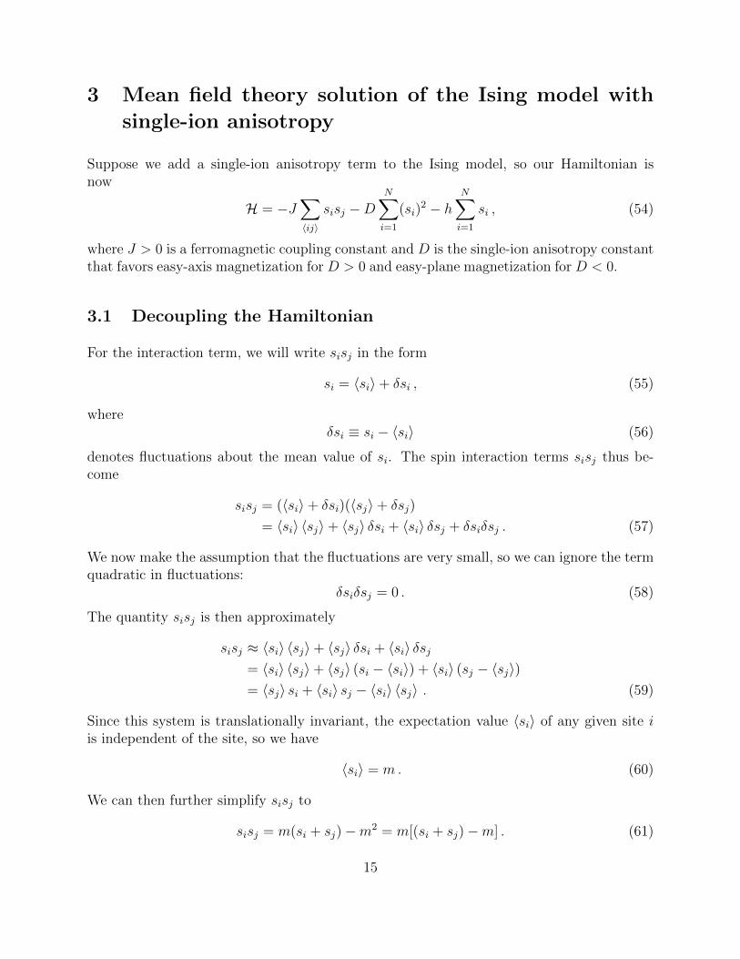
where J > 0 is a ferromagnetic coupling constant and D is the single-ion anisotropy constantthat favors easy-axis magnetization for D > 0 and easy-plane magnetization for D < 0.

3.1 Decoupling the Hamiltonian

For the interaction term, we will write sisj in the form

si = 〈si〉+ δsi , (55)

whereδsi ≡ si − 〈si〉 (56)

denotes fluctuations about the mean value of si. The spin interaction terms sisj thus be-come

sisj = (〈si〉+ δsi)(〈sj〉+ δsj)

= 〈si〉 〈sj〉+ 〈sj〉 δsi + 〈si〉 δsj + δsiδsj . (57)

We now make the assumption that the fluctuations are very small, so we can ignore the termquadratic in fluctuations:

δsiδsj = 0 . (58)

The quantity sisj is then approximately

sisj ≈ 〈si〉 〈sj〉+ 〈sj〉 δsi + 〈si〉 δsj= 〈si〉 〈sj〉+ 〈sj〉 (si − 〈si〉) + 〈si〉 (sj − 〈sj〉)= 〈sj〉 si + 〈si〉 sj − 〈si〉 〈sj〉 . (59)

Since this system is translationally invariant, the expectation value 〈si〉 of any given site iis independent of the site, so we have

〈si〉 = m. (60)

We can then further simplify sisj to

sisj = m(si + sj)−m2 = m[(si + sj)−m] . (61)

15

Similarly, for the single-ion anisotropy term, we will write (si)2 as

(si)2 = 2msi −m2 = m(2si −m) . (62)

The mean field Hamiltonian is then

HMF = −Jm∑〈ij〉

(si + sj −m)−DmN∑i=1

(2si −m)− hN∑i=1

si

= −Jm∑〈ij〉

(2si −m)−DmN∑i=1

(2si −m)− hN∑i=1

si

= −qJm2

N∑i=1

(2si −m)−DmN∑i=1

(2si −m)− hN∑i=1

si

=

(qJ

2+D

)Nm2 − [h+ (qJ + 2D)m]

N∑i=1

si ,

where q is the coordination number. We thus find

HMF =

(qJ

2+D

)Nm2 − heff

N∑i=1

si , (63)

whereheff ≡ h+ (qJ + 2D)m (64)

is the effective magnetic field felt by the spins.

3.2 Self-consistency equation

Let’s calculate the partition function using the mean field Hamiltonian:

ZMF = Tr(e−βHMF)

=N∏i=1

(∑si=±1

)e−βHMF

=N∏i=1

(∑si=±1

)e−β( qJ

2+D)Nm2

eβheff∑N

j=1 sj

= e−β( qJ2

+D)Nm2N∏i=1

(∑si=±1

eβheffsi

)

= e−β( qJ2

+D)Nm2N∏i=1

(eβheff + e−βheff)︸ ︷︷ ︸=2 cosh(βheff)

= e−β( qJ2

+D)Nm2

[2 cosh(βheff)]N , (65)

16

so we find

ZMF = e−β( qJ2

+D)Nm2

[2 cosh(βheff)]N . (66)

Now, recall from Eq. 2 that the magnetization is given by

m ≡ 1

N

N∑i=1

〈si〉 .

Using Eq. 3, we can rewrite this as

m =1

N

N∑i=1

Tr(sie−βHMF)

ZMF

=1

N

1

ZMF

N∑i=1

sie−βHMF

=1

Nβ

1

ZMF

∂ZMF

∂heff

=1

Nβ

∂(lnZMF)

∂heff

, (67)

where on the third line we have used the fact that

∂ZMF

∂heff

=∂

∂heff

Tr(e−βHMF)

= Tr

(∂

∂heff

e−βHMF

)= −β Tr

(∂HMF

∂heff

e−βHMF

)= −β Tr

[(−

N∑i=1

si

)e−βHMF

]

= β Tr

[N∑i=1

sie−βHMF

]. (68)

Now, from Eq. 66 we can calculate lnZMF:

lnZMF = −β(qJ

2+D

)Nm2 +N ln 2 +N ln[cosh(βheff)] , (69)

so∂(lnZMF)

∂heff

= Nβ tanh(βheff) . (70)

Inserting this back into Eq. 67 gives

m = tanh(βheff) . (71)

17

Inserting the definition of heff (Eq. 64) back into this equation gives us the self-consistencyequation

m = tanh[β(h+ (qJ + 2D)m

)]. (72)

This corresponds to a system with a phase transition at kBTc = qJ + 2D. Above thistemperature, it is paramagnetic, and below this temperature, it is ferromagnetic. Note thatthe system will be paramagnetic for all (nonzero) temperatures if D < −qJ/2 (rememberthat D < 0 favors easy-plane magnetization).

References

[1] Mean-Field Theory. https://www.physik.uni-muenchen.de/lehre/vorlesungen/

sose_14/asp/lectures/ASP_Chapter5.pdf.

[2] Martin Evans. Mean-Field Theory of the Ising Model. https://www2.ph.ed.ac.uk/

~mevans/sp/sp10.pdf.

18