monografia
DESCRIPTION
Strong Floor DesignTRANSCRIPT

Seediscussions,stats,andauthorprofilesforthispublicationat:https://www.researchgate.net/publication/265293302
DESIGNOFALARGE-SCALEDYNAMICANDPSEUDO-DYNAMICTESTINGFACILITY
BOOK·JULY2005
DOI:10.13140/2.1.3557.3121
CITATIONS
6
READS
75
5AUTHORS,INCLUDING:
G.M.Calvi
IstitutoUniversitariodiStudiSuperioridiP…
121PUBLICATIONS2,493CITATIONS
SEEPROFILE
AlbertoPavese
UniversityofPavia
42PUBLICATIONS173CITATIONS
SEEPROFILE
PaolaCeresa
IstitutoUniversitariodiStudiSuperioridiP…
13PUBLICATIONS101CITATIONS
SEEPROFILE
Availablefrom:AlbertoPavese
Retrievedon:12January2016
DESIGN OF A LARGE-SCALE DYNAMIC AND PSEUDO-DYNAMIC TESTING
FACILITY
Gian Michele Calvi Professor of Structural Engineering
University of Pavia, Department of Structural Mechanics
Alberto Pavese Associate Professor
University of Pavia, Department of Structural Mechanics
Paola Ceresa Doctoral Student
European School for Advanced Studies in Reduction of Seismic Risk
Filippo Dacarro Laboratory Engineer
European Centre for Training and Research in Earthquake Engineering
Carlo G. Lai Associate Researcher
European Centre for Training and Research in Earthquake Engineering
Carlo Beltrami Graduate Researcher
European School for Advanced Studies in Reduction of Seismic Risk
Pavia, Italy, July 2005

Nessuna parte di questo libro può essere riprodotta o trasmessa in qualsiasi forma o con qualsiasi mezzo elettronico, meccanico o altro senza l’autorizzazione scritta dei proprietari dei diritti e dell’editore.
©Copyright 2005 - IUSS Press
prodotto da: Multimedia Cardano
Via Cardano, 14 - 27100 Pavia, Italy Tel.: (+39) 0382.539776 - fax: (+39) 0382.306406 - e-mail: [email protected]
distribuito da: IUSS Press
IUSS, Collegio Giasone del Maino, Via Luino, 4 - 27100 Pavia, Italy Tel.: (+39) 0382.375841 - fax: (+39) 0382.375899 - email: [email protected] - web: www.iusspress.it
PREFACE This manuscript provides a relatively detailed description of the design of the high-performance uniaxial shaking table as well as of the reaction walls and strong floor at the European Centre for Training and Research in Earthquake Engineering (EUCENTRE, Pavia, Italy). The latter was founded by the Italian National Civil Protection Department, the Italian National Institute for Geophysics and Volcanology, the University of Pavia and the Institute for Advanced Study of Pavia, under the main financial backing of the first of these four partners. The work described in the current publication has benefited significantly from the input of a number of collaborators who have worked closely with the authors in the design of the dynamic and pseudo-dynamic testing facility. Within this context, the following contributors are acknowledged: • Ms. Maria Pia Scovenna for the precious and most valuable assistance with the analysis
and design of the laboratory, the preparation of a very large number of technical drawings and the set-up and construction of the laboratory;
• Dr. Claudio Strobbia, for his contribution to the studies that targeted the evaluation of the dynamic soil-structure interaction effects;
• Ms. Maria Rota, for her contribution to the structural analyses of the testing facilities; • Mr. Paolo Paruta, from Tecno-cut Srl, Mr. Gianni Lova, from Hydros Srl, Mr. Al J.
Clark, Mr. Dave Kusner and Mr. Carlo Maria Ornati, all from MTS Systems Corporation, for their important roles in the design of the shaking table and pseudo-dynamic testing facilities;
• the staff at Cielle Prefabbricati SpA, at Ninive Casseformi Srl and at Alga SpA, for the physical construction of the laboratory, a task for which the contribution of lab technicians Mr. Michele D’Adamo and Mr. Franco Barzon is also very much acknowledged.
The authors would also like to thank Dr. Rui Pinho, for his assistance in the organisation and writing-up of this report, as well as Mr. Arun Menon, who kindly volunteered to proof-review the final draft of this manuscript. The contributions of Dr. Adam J. Crewe and Dr. Giovanni Fabbrocino, who kindly providing material related to the shaking tables of the University of Bristol (UK) and University of Naples “Federico II” (Italy), respectively, are also gratefully acknowledged. Finally, it is noted that the project has also benefited from the active cooperation with Reluis, the Italian National Network of Earthquake Engineering University Laboratories.

TABLE OF CONTENTS
Preface .............................................................................................................................................. iii Table of contents ............................................................................................................................. v List of figures................................................................................................................................... ix List of tables ................................................................................................................................... xv Chapter 1 : Introduction................................................................................................................. 1 1.1 Overview...................................................................................................................................1 1.2 Objectives and outline ............................................................................................................2 Chapter 2 : The new EUCENTRE facility.................................................................................. 5 2.1 Shaking table testing................................................................................................................5
2.1.1 Some existing facilities ..................................................................................................6 2.1.2 Summary of main features of existing shaking tables ............................................13
2.2 Pseudo-dynamic testing........................................................................................................14 2.2.1 Some existing facilities ................................................................................................16 2.2.2 Summary of main features of existing pseudo-dynamic (PsD) facilities.............18
2.3 Definition of the new EUCENTRE testing facility performance targets....................19 2.3.1 Local needs and constraints .......................................................................................19 2.3.2 General description of the EUCENTRE dynamic testing facility
requirements................................................................................................................20 2.3.3 General description of the EUCENTRE pseudo-dynamic testing facility
requirements................................................................................................................23 Chapter 3 : Design of the dynamic testing facility....................................................................25 3.1 Relevant issues for the design of the dynamic testing facility ........................................25
3.1.1 Specifications for the shaking table design ..............................................................25 3.1.2 Specifications for the system restraining the platform motion ............................28 3.1.3 Specifications for the reaction mass design .............................................................30 3.1.4 Specifications for the isolation and damping system design.................................31 3.1.5 Regions of flexibility....................................................................................................33
3.2 Design of the structural and mechanical arrangement of the shaking table ................33 3.2.1 Final configuration of the EUCENTRE shaking table .........................................33 3.2.2 Design revision history ...............................................................................................40
3.3 Design of the system restraining the motion of the platform........................................41 3.3.1 Final configuration.......................................................................................................41 3.3.2 Design revision history ...............................................................................................46
3.4 Design of the reaction mass.................................................................................................46 3.4.1 Final configuration.......................................................................................................46 3.4.2 Design revision history ...............................................................................................49
3.5 Design of the isolation system ............................................................................................51 3.5.1 Final solution ................................................................................................................51
Design of a large-scale dynamic and pseudo-dynamic testing facility
vi
3.5.2 Design revision history ...............................................................................................52 3.6 Numerical verifications.........................................................................................................53
3.6.1 Dynamic response characteristics .............................................................................53 3.6.2 Deformability of the testing system..........................................................................57 3.6.3 Short pier: overturning moment effects...................................................................61 3.6.4 Tall pier: overturning moment effects......................................................................65 3.6.5 Short and tall piers: overturning moment and longitudinal force effects ...........67 3.6.6 Effects of the maximum design loads ......................................................................71
Chapter 4 : Design of the pseudo-dynamic testing facility ..................................................... 75 4.1 Relevant issues for the design of the PsD facility ............................................................75 4.2 Design of the structural arrangement of the EUCENTRE PsD apparatus ................76 4.3 Stiffness evaluation of the PsD apparatus.........................................................................77 4.4 Design of the post-tensioning system................................................................................82 4.5 Design of the foundation system........................................................................................93 4.6 Design revision history .........................................................................................................96 Chapter 5 : Actuator system.......................................................................................................101 5.1 Applications of external actions........................................................................................101 5.2 Actuator system of the shaking table ...............................................................................104 5.3 Actuator system of the PsD facility..................................................................................111 5.4 Generation and distribution of the pressurized oil ........................................................112 Chapter 6 : Soil-structure interaction .......................................................................................115 6.1 Aspects of soil-structure interaction investigations .......................................................115 6.2 Definition of dynamic properties of foundation soil ....................................................116 6.3 Static vertical settlement.....................................................................................................119
6.3.1 Theoretical background ............................................................................................119 6.3.2 Static vertical settlement due to the shaking table weight ...................................125 6.3.3 Static vertical settlement due to PsD testing apparatus weight ..........................131
6.4 Dynamic soil-structure interaction problem ...................................................................136 6.4.1 Dynamic soil-structure interaction..........................................................................136 6.4.2 Evaluation of liquefaction potential........................................................................149
Chapter 7 : Closure......................................................................................................................153 7.1 Design of the testing facility ..............................................................................................153
7.1.1 Design of the shaking table......................................................................................153 7.1.2 Design of the PsD apparatus ...................................................................................153 7.1.3 Soil-structure interaction problem ..........................................................................153
7.2 Future work ..........................................................................................................................154 References.....................................................................................................................................155 APPENDIX A – Choice of the structural layout ..................................................................163 APPENDIX B – Welding technology for the EUCENTRE shaking table ......................167
Table of Contents
vii
APPENDIX C – Characteristics of the selected accelerograms..........................................171 APPENDIX D – Tensile and compressive stresses for the PsD apparatus (Figure 4.4 and Figure 4.5) .............................................................................................................................173 APPENDIX E – Top wall and top pier displacements for the final PsD configuration (Figure 4.3)....................................................................................................................................175 APPENDIX F – Wall displacements at the top and at the force application joints for 1st possible PsD configuration (Figure 4.23) ...........................................................................177

LIST OF FIGURES Figure 2.1 Schematic arrangement of the Master shaking table [ECOEST, 1997]............... 8 Figure 2.2 Arrangement of the three-axis table at LNEC [ECOEST, 1997]......................... 9 Figure 2.3 Arrangement of the six-axes table in Athens [ECOEST, 1997] .........................10 Figure 2.4 Arrangement of the six-axis table in Bristol [ECOEST, 1997] ...........................11 Figure 2.5 The outdoor shaking table at the University of California, San Diego [Van
Den Einde et al., 2004].............................................................................................12 Figure 2.6 An outline of the shaking table system at Miki City [Ogawa et al., 2001] ..........13 Figure 2.7 Reaction-wall at the ELSA laboratory [adapted from Joint Research Centre
- ELSA, 1999] ...........................................................................................................16 Figure 2.8 Multi-Axial Subassemblage Testing (MAST) System [French et al., 2004] ........18 Figure 2.9 Honeycomb-like network of stiffening diaphragms: one possible solution......22 Figure 3.1 Overturning moment contributions. (a) Sum and (b) subtraction of the
contributions of the inertial forces ........................................................................27 Figure 3.2 Possible solution for the hydrostatic bearings .......................................................28 Figure 3.3 Front view of the guide, and bearing areas.............................................................29 Figure 3.4 Guides: side view ........................................................................................................29 Figure 3.5 Components of a typical shaking table [Clark, 1992]............................................32 Figure 3.6 Potential regions of flexibility in a typical shaking table [Crewe, 1998] .............33 Figure 3.7 Final configuration of the shaking table: locations of the hydrostatic
bearings ......................................................................................................................34 Figure 3.8 Honey-comb like network of stiffening diaphragms of the final
configuration: different views (a), (b) and (c) ......................................................36 Figure 3.9 One transversal section of the EUCENTRE shaking table ................................37 Figure 3.10 Plan view of the shaking table without the top plate..........................................37 Figure 3.11 Additional wings to increase the table width from 4000 mm to 5600 mm.....38 Figure 3.12 Sequence of composition by welding....................................................................39 Figure 3.13 Final hydrostatic and mechanical solution to avoid table deformations .........42 Figure 3.14 Bearing friction force vs. shaking table velocity ..................................................43 Figure 3.15 Tolerance errors specified to the manufacturer. Dimensions in mm ..............43 Figure 3.16 Plan view of the anchorage points (circles sign the M60 high-strength
bars) ............................................................................................................................44 Figure 3.17 Sectional views of the first and third fixed guides...............................................45 Figure 3.18 Final configuration of the reaction mass (without the added precast blocks
at the two ends).........................................................................................................48 Figure 3.19 Construction procedure to cast BW-Fixators-RK within reaction mass
(dimensions in cm) ...................................................................................................49 Figure 3.20 First investigated shape of the reaction mass.......................................................50 Figure 3.21 Layout of the isolation system considering T29 CF_Gomma model: 150
air springs...................................................................................................................52 Figure 3.22 First mode shape of the final configuration (deformations in mm). Perfect
restraints.....................................................................................................................54
Design of a large-scale dynamic and pseudo-dynamic testing facility
x
Figure 3.23 Mode shapes of the final configuration (deformations in mm), equivalent springs, middle-stroke position .............................................................................. 54
Figure 3.24 Mode shapes of the final configuration (deformations in mm), equivalent springs, end-stroke position.................................................................................... 55
Figure 3.25 First mode shape: table loaded with the maximum payload at 1 m and 7 m..56 Figure 3.26 Possible effective mass of a specimen for different peak accelerations .......... 58 Figure 3.27 OTM at the table base for different peak accelerations ..................................... 58 Figure 3.28 Shaking table position in the middle of the fixed guides ................................... 60 Figure 3.29 Shaking table position at the end of the fixed guides ......................................... 60 Figure 3.30 Deformed shape: OTM effect due to short pier, middle stroke position ....... 63 Figure 3.31 Short pier. OTM effect: vertical deformations of the bearings (z = -1.7 m,
-1.5 m and -1.1 m), middle stroke position .......................................................... 63 Figure 3.32 Deformed shape: OTM effect due to short pier, end stroke position............. 64 Figure 3.33 Short pier. OTM effect: vertical deformations of the bearings (z = -1.7 m,
-1.5 m and -1.1 m), end stroke position................................................................ 64 Figure 3.34 Deformed shape: OTM effect due to tall pier, middle stroke position ........... 66 Figure 3.35 Tall pier. OTM effect: vertical deformations of the bearings (z = -1.7 m, -
1.5 m and -1.1 m), middle stroke position ........................................................... 66 Figure 3.36 Deformed shape: OTM effect due to tall pier, end stroke position................. 67 Figure 3.37 Tall pier. OTM effect: vertical deformations of the bearings (z = -1.7 m, -
1.5 m and -1.1 m), end stroke position ................................................................. 67 Figure 3.38 Short pier. OTM effect: vertical deformations of the bearings (z = -1.7 m,
-1.5 m and -1.1 m). Middle (a) and end (b) stroke positions. Maximum longitudinal force applied........................................................................................ 69
Figure 3.39 Tall pier. OTM effect: vertical deformations of the bearings (z = -1.7 m, -1.5 m and -1.1 m). Middle (a) and end (b) stroke positions. Maximum longitudinal force applied........................................................................................ 70
Figure 3.40 Deformed shape due to maximum design load application, middle stroke position ...................................................................................................................... 72
Figure 3.41 Design load effect: vertical deformations of the bearings (z = -1.7 m, -1.5 m and -1.1 m), middle stroke position.................................................................. 72
Figure 3.42 Von Mises stresses due to maximum design load application, middle stroke position .......................................................................................................... 73
Figure 3.43 Deformed shape due to maximum design load application, end stroke position ...................................................................................................................... 73
Figure 3.44 Design load effect: vertical deformations of the bearings (z = -1.7 m, -1.5 m and -1.1 m), end stroke position ....................................................................... 74
Figure 3.45 Von Mises stresses due to maximum design load application, end stroke position ...................................................................................................................... 74
Figure 4.1 Final configuration of the PsD test apparatus: view in plan................................ 77 Figure 4.2 Pier cross section: three different longitudinal reinforcement percentages
(scaled 1:2) ................................................................................................................. 79 Figure 4.3 Final PsD structural configuration: 3D view ......................................................... 81
List of Figures
xi
Figure 4.4 Stress field for the shorter wall (9.6 m) of the final PsD configuration.............81 Figure 4.5 Stress field for the longer wall (14.4 m) of the final PsD configuration............82 Figure 4.6 Mechanical stressing anchorage types “M” [Alga, 2004]......................................83 Figure 4.7 Stressing anchorage type “M” [Alga, 2004] ............................................................85 Figure 4.8 Cross-section of the precast block with the perforations for the 31T15
tendons.......................................................................................................................86 Figure 4.9 Stress trend: each wall subjected to its maximum forces .....................................88 Figure 4.10 Strong floor: directions of the hollow precast blocks.........................................90 Figure 4.11 Full view of the PsD apparatus after the design of cable location ...................90 Figure 4.12 Detailed view of the 14.4 m long wall: vertical and transversal cable
locations .....................................................................................................................91 Figure 4.13 Detailed view of 9.6 m long wall: vertical and transversal cable locations......91 Figure 4.14 Detailed view of the strong floor: horizontal cable locations ...........................92 Figure 4.15 Block type A ..............................................................................................................92 Figure 4.16 Block Type D ............................................................................................................92 Figure 4.17 Block Type E.............................................................................................................93 Figure 4.18 Block Type G ............................................................................................................93 Figure 4.19 Schematically in plan view of the foundation system for the PsD
apparatus ....................................................................................................................94 Figure 4.20 Strong floor and foundation system: final configuration (SAP [Computer
and Structures, Inc., 1995]) .....................................................................................95 Figure 4.21 View of the foundation system beneath the strong floor (finite element
mesh with SAP [Computer and Structures, Inc., 1995]) ....................................96 Figure 4.22 Initially investigated configuration of the PsD test apparatus: plan view........97 Figure 4.23 Initially investigated PsD structural configuration: 3D view.............................98 Figure 4.24 Approximate verification of the FE model results .............................................98 Figure 4.25 Stress field for the shorter wall (9.6 m) of the 1st PsD configuration ..............99 Figure 4.26 Stress field for the longer wall (12 m) of the 1st PsD configuration.................99 Figure 5.1 Performance curves for the hydraulic actuator....................................................105 Figure 5.2 Hydraulic actuator assembly by MTS System Corporation [2004] ...................106 Figure 5.3 Cylinder assembly by MTS System Corporation [2004].....................................107 Figure 5.4 Actuator interfaces by Tecno-cut [2004]...............................................................109 Figure 5.5 Square steel plate at the interface reaction mass/actuator .................................109 Figure 5.6 Actuator interfaces by MTS System Corporation [2004] ...................................110 Figure 5.7 Piping system for the EUCENTRE laboratory [Hydros s.r.l., 2004]...............113 Figure 6.1 Blow/foot values from the standard penetration tests.......................................117 Figure 6.2 Shear wave velocity profile from the SPT tests ...................................................118 Figure 6.3 Profiles of P and S wave velocities (left). Poisson’s ratio profile with depth
(right) ........................................................................................................................119 Figure 6.4 Experimental Vs profile with the standard deviation values with depth. On
the right hand side, the Vs precautionary design profile for static loading conditions is shown................................................................................................120
Design of a large-scale dynamic and pseudo-dynamic testing facility
xii
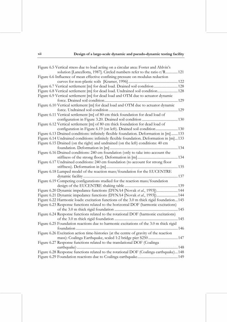
Figure 6.5 Vertical stress due to load acting on a circular area: Foster and Ahlvin’s solution [Lancellotta, 1987]. Circled numbers refer to the ratio r/R.............121
Figure 6.6 Influence of mean effective confining pressure on modulus reduction curves for non-plastic soils [Kramer, 1996] ......................................................122
Figure 6.7 Vertical settlement [m] for dead load. Drained soil condition ..........................128 Figure 6.8 Vertical settlement [m] for dead load. Undrained soil condition......................128 Figure 6.9 Vertical settlement [m] for dead load and OTM due to actuator dynamic
force. Drained soil condition................................................................................129 Figure 6.10 Vertical settlement [m] for dead load and OTM due to actuator dynamic
force. Undrained soil condition ...........................................................................129 Figure 6.11 Vertical settlement [m] of 80 cm thick foundation for dead load of
configuration in Figure 3.20. Drained soil condition .......................................130 Figure 6.12 Vertical settlement [m] of 80 cm thick foundation for dead load of
configuration in Figure 6.19 (on left). Drained soil condition........................130 Figure 6.13 Drained conditions: infinitely flexible foundation. Deformation in [m] .......133 Figure 6.14 Undrained conditions: infinitely flexible foundation. Deformation in [m]...133 Figure 6.15 Drained (on the right) and undrained (on the left) conditions: 40 cm
foundation. Deformation in [m] ..........................................................................134 Figure 6.16 Drained conditions: 240 cm foundation (only to take into account the
stiffness of the strong floor). Deformation in [m]............................................134 Figure 6.17 Undrained conditions: 240 cm foundation (to account for strong floor
stiffness). Deformation in [m]..............................................................................135 Figure 6.18 Lumped model of the reaction mass/foundation for the EUCENTRE
dynamic facility .......................................................................................................137 Figure 6.19 Competing configurations studied for the reaction mass/foundation
design of the EUCENTRE shaking table ..........................................................139 Figure 6.20 Dynamic impedance functions (DYNA4 [Novak et al., 1993]).......................144 Figure 6.21 Dynamic impedance functions (DYNA4 [Novak et al., 1993]).......................144 Figure 6.22 Harmonic loads: excitation functions of the 3.0 m thick rigid foundation...145 Figure 6.23 Response functions related to the horizontal DOF (harmonic excitations)
of the 3.0 m thick rigid foundation .....................................................................145 Figure 6.24 Response functions related to the rotational DOF (harmonic excitations)
of the 3.0 m thick rigid foundation .....................................................................145 Figure 6.25 Foundation reactions due to harmonic excitations of the 3.0 m thick rigid
foundation ...............................................................................................................146 Figure 6.26 Excitation action time-histories (at the centre of gravity of the reaction
mass): Coalinga Earthquake, scaled 1:2 bridge pier S250 ................................147 Figure 6.27 Response functions related to the translational DOF (Coalinga
earthquake) ..............................................................................................................148 Figure 6.28 Response functions related to the rotational DOF (Coalinga earthquake)...148 Figure 6.29 Foundation reactions due to Coalinga earthquake............................................149
List of Figures
xiii
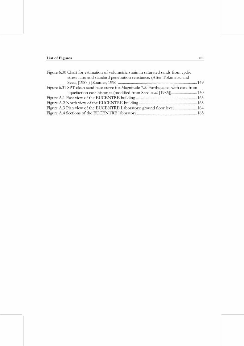
Figure 6.30 Chart for estimation of volumetric strain in saturated sands from cyclic stress ratio and standard penetration resistance. (After Tokimatsu and Seed, [1987]) [Kramer, 1996] ................................................................................149
Figure 6.31 SPT clean-sand base curve for Magnitude 7.5. Earthquakes with data from liquefaction case histories (modified from Seed et al. [1985])..........................150
Figure A.1 East view of the EUCENTRE building ..............................................................163 Figure A.2 North view of the EUCENTRE building ...........................................................163 Figure A.3 Plan view of the EUCENTRE Laboratory: ground floor level .......................164 Figure A.4 Sections of the EUCENTRE laboratory .............................................................165

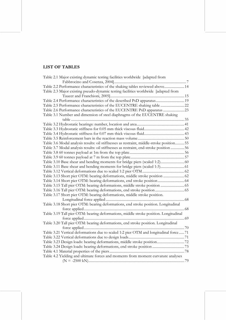
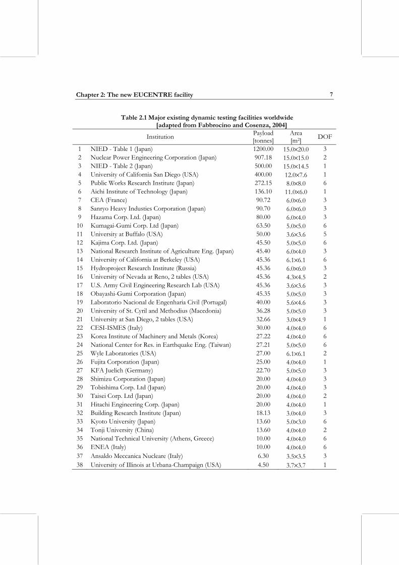
LIST OF TABLES Table 2.1 Major existing dynamic testing facilities worldwide [adapted from
Fabbrocino and Cosenza, 2004]............................................................................... 7 Table 2.2 Performance characteristics of the shaking tables reviewed above......................14 Table 2.3 Major existing pseudo-dynamic testing facilities worldwide [adapted from
Taucer and Franchioni, 2005].................................................................................15 Table 2.4 Performance characteristics of the described PsD apparatus ...............................19 Table 2.5 Performance characteristics of the EUCENTRE shaking table ..........................22 Table 2.6 Performance characteristics of the EUCENTRE PsD apparatus .......................23 Table 3.1 Number and dimension of steel diaphragms of the EUCENTRE shaking
table ............................................................................................................................35 Table 3.2 Hydrostatic bearings: number, location and area....................................................41 Table 3.3 Hydrostatic stiffness for 0.05 mm thick viscous fluid............................................42 Table 3.4 Hydrostatic stiffness for 0.07 mm thick viscous fluid............................................43 Table 3.5 Reinforcement bars in the reaction mass volume...................................................50 Table 3.6 Modal analysis results: oil stiffnesses as restraint, middle-stroke position..........55 Table 3.7 Modal analysis results: oil stiffnesses as restraint, end-stroke position ...............56 Table 3.8 60 tonnes payload at 1m from the top plate............................................................56 Table 3.9 60 tonnes payload at 7 m from the top plate...........................................................57 Table 3.10 Base shear and bending moments for bridge piers (scaled 1:2)..........................60 Table 3.11 Base shear and bending moments for bridge piers (scaled 1:3)..........................61 Table 3.12 Vertical deformations due to scaled 1:2 pier OTM..............................................62 Table 3.13 Short pier OTM: bearing deformations, middle stroke position .......................62 Table 3.14 Short pier OTM: bearing deformations, end stroke position .............................64 Table 3.15 Tall pier OTM: bearing deformations, middle stroke position ..........................65 Table 3.16 Tall pier OTM: bearing deformations, end stroke position ................................65 Table 3.17 Short pier OTM: bearing deformations, middle stroke position.
Longitudinal force applied ......................................................................................68 Table 3.18 Short pier OTM: bearing deformations, end stroke position. Longitudinal
force applied..............................................................................................................68 Table 3.19 Tall pier OTM: bearing deformations, middle stroke position. Longitudinal
force applied..............................................................................................................69 Table 3.20 Tall pier OTM: bearing deformations, end stroke position. Longitudinal
force applied..............................................................................................................70 Table 3.21 Vertical deformations due to scaled 1:2 pier OTM and longitudinal force......71 Table 3.22 Vertical deformations due to design loads.............................................................71 Table 3.23 Design loads: bearing deformations, middle stroke position..............................72 Table 3.24 Design loads: bearing deformations, end stroke position ...................................73 Table 4.1 Material properties of the piers..................................................................................78 Table 4.2 Yielding and ultimate forces and moments from moment curvature analyses
(N = -2500 kN).........................................................................................................79
Design of a large-scale dynamic and pseudo-dynamic testing facility
xvi
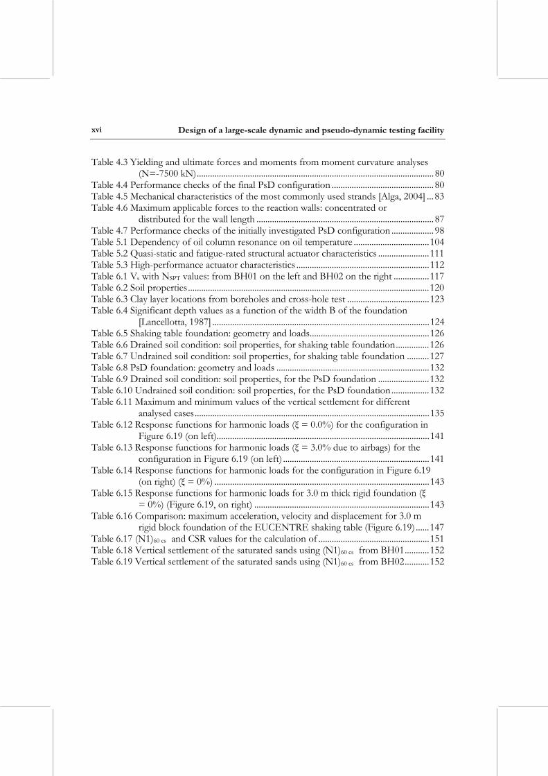
Table 4.3 Yielding and ultimate forces and moments from moment curvature analyses (N=-7500 kN)........................................................................................................... 80
Table 4.4 Performance checks of the final PsD configuration .............................................. 80 Table 4.5 Mechanical characteristics of the most commonly used strands [Alga, 2004] ... 83 Table 4.6 Maximum applicable forces to the reaction walls: concentrated or
distributed for the wall length ................................................................................ 87 Table 4.7 Performance checks of the initially investigated PsD configuration ................... 98 Table 5.1 Dependency of oil column resonance on oil temperature ..................................104 Table 5.2 Quasi-static and fatigue-rated structural actuator characteristics .......................111 Table 5.3 High-performance actuator characteristics ............................................................112 Table 6.1 Vs with NSPT values: from BH01 on the left and BH02 on the right ................117 Table 6.2 Soil properties.............................................................................................................120 Table 6.3 Clay layer locations from boreholes and cross-hole test .....................................123 Table 6.4 Significant depth values as a function of the width B of the foundation
[Lancellotta, 1987] ..................................................................................................124 Table 6.5 Shaking table foundation: geometry and loads......................................................126 Table 6.6 Drained soil condition: soil properties, for shaking table foundation...............126 Table 6.7 Undrained soil condition: soil properties, for shaking table foundation ..........127 Table 6.8 PsD foundation: geometry and loads .....................................................................132 Table 6.9 Drained soil condition: soil properties, for the PsD foundation .......................132 Table 6.10 Undrained soil condition: soil properties, for the PsD foundation.................132 Table 6.11 Maximum and minimum values of the vertical settlement for different
analysed cases..........................................................................................................135 Table 6.12 Response functions for harmonic loads (ξ = 0.0%) for the configuration in
Figure 6.19 (on left)................................................................................................141 Table 6.13 Response functions for harmonic loads (ξ = 3.0% due to airbags) for the
configuration in Figure 6.19 (on left) ..................................................................141 Table 6.14 Response functions for harmonic loads for the configuration in Figure 6.19
(on right) (ξ = 0%) .................................................................................................143 Table 6.15 Response functions for harmonic loads for 3.0 m thick rigid foundation (ξ
= 0%) (Figure 6.19, on right) ...............................................................................143 Table 6.16 Comparison: maximum acceleration, velocity and displacement for 3.0 m
rigid block foundation of the EUCENTRE shaking table (Figure 6.19) ......147 Table 6.17 (N1)60 cs and CSR values for the calculation of ..................................................151 Table 6.18 Vertical settlement of the saturated sands using (N1)60 cs from BH01...........152 Table 6.19 Vertical settlement of the saturated sands using (N1)60 cs from BH02...........152
CHAPTER 1: INTRODUCTION
1.1 OVERVIEW Structural behaviour under dynamic loads is vital in many branches of civil, mechanical and aerospace engineering. Examples include earthquake loading of buildings, vibration induced by vehicles on non-uniform road surfaces and launching loads in spacecraft. All these applications share the common characteristics that they are difficult to model analytically and that detailed monitoring of prototype structures in the field is uneconomic and in many cases impossible. Laboratory testing therefore has a crucial role to play in furthering our understanding of dynamic loads and mitigating their undesirable effects. The present work is focused on earthquake engineering. The key issue in any laboratory test is the accuracy with which the conditions in the field can be reproduced. If the laboratory conditions are not representative, then the test results will at best be of limited applicability, and may be dangerously misleading. An accurate dynamic test requires very high performance of three main elements: the hardware used to apply the loads (usually servo-hydraulic actuators); the control system that monitors and corrects the loads; and (in the case of hybrid methods such as pseudo-dynamic testing) the numerical dynamic analysis that runs in parallel with the physical test. In civil engineering, scaling and rate of loading effects are particularly problematic. Extrapolating from small-scale model results to prototype behaviour is fraught with difficulties, particularly when the structural response is nonlinear. However, loading full-scale structures at the correct rate requires enormous resources and extremely high-performance hardware. Some compromise is therefore usually necessary. In the field of earthquake engineering, the most widely used experimental methods are the following [Carvalho, 1998]: • Static cyclic testing is widely used for determining the performance of materials and
elements under the repeated load reversals that occur during earthquakes, though it does not model dynamic behaviour.
• Shaking tables are widely used to impose prescribed base motions on reduced-scale models, though a few tables exist which have the capacity to apply seismic base motions to full-scale structures, as described later. Apart from the scaling problems mentioned above, there are difficulties in controlling such tests. Traditional control
Design of a large-scale dynamic and pseudo-dynamic testing facility
2
algorithms require a priori knowledge of the properties of the system being controlled. However, these are generally not known to a high degree of accuracy and may change during the test as the specimen suffers damage.
• The main current alternative to shaking table testing is pseudo-dynamic (PsD) testing in which a large-scale test specimen is loaded over an expanded time-scale with the dynamic effects accounted for computationally. This is acceptable if the dynamic and rate-dependent effects can be calculated reliably but, uncertainty over these aspects of behaviour is very often the motivation for performing the test in the first place.
• More recently, a variety of real-time methods have been developed. Like pseudo-dynamic testing, these use a combination of physical testing and numerical modelling, but the experimental part of the process is performed at the correct rate so that the test specimen can respond dynamically [Nakashima et al., 1990].
• Arrays of explosive charges are occasionally used to simulate earthquake ground motions at large scale [Kitada et al., 2000].
• Dynamic centrifuge testing is used to model geotechnical and soil-structure interaction problems.
Among such methods, static cyclic testing does not involve dynamics, array of explosive charges is a rather infrequently used approach, and dynamic centrifuge testing is used in the testing of soils.
1.2 OBJECTIVES AND OUTLINE This manuscript focuses on the design of a new testing facility to be constructed at the European Centre for Training and Research in Earthquake Engineering (EUCENTRE) in Pavia (Italy). The design of both shaking table and pseudo-dynamic testing facilities is discussed. The testing element capabilities are given, focusing on the servo-hydraulic actuator performances for both dynamic and pseudo-dynamic testing. The problem of soil-structure interaction has been studied in terms of the settlements due to the static loads for both the shaking table and the PsD apparatus. The dynamic resultant motion transmitted to the soil from the shaking table is taken into account. The seismic isolation of the shaking table, and consequently of the overall structure, is studied. This publication is organized as follows. Chapter two introduces the testing facility under construction at the EUCENTRE. In particular, an overview of the dynamic and pseudo-dynamic testing is given. Some examples of existing shaking tables and pseudo-dynamic apparatus are given. The testing facility performance targets are discussed in comparison with the local needs and constraints. Chapter three describes the design of the EUCENTRE shaking table, with particular attention to the structural and mechanical arrangements of the platform, the stiffness
Chapter 1: Introduction
3
evaluation of the system restraining the platform motion, the design of the reaction mass and the isolation system. Chapter four describes the design of the EUCENTRE pseudo-dynamic testing facility. The structural arrangement of the PsD apparatus is described and the evaluation of its stiffness is presented. The design of the post-tensioning system for the reaction walls and the strong floor is described. The foundation system of the facility is designed to take into account the anchorage spaces of the cables. Chapter five is a brief description of the testing elements such as the servo-hydraulic actuators. The performance characteristics of the powerful actuator of the shaking table are listed together with the actuators required for the PsD apparatus. The piping system for both facilities is briefly described. Chapter six is devoted to the study of the soil-structure interaction: both soil-shaking table and soil-PsD apparatus interaction. The soil properties are described. The evaluation of the vertical settlements due to static loads is performed under the reaction mass of the shaking table and the PsD apparatus, respectively. From a dynamic point of view, the complex interaction due the table’s resultant motion transmitted to the underlying soil is developed with reference to the work of Pavese et al. [2005]. Chapter seven provides a succinct closure to this manuscript.

CHAPTER 2: THE NEW EUCENTRE FACILITY
In this chapter, the rationale behind the construction of the new testing facility at the EUCENTRE is presented. This requires, however, that a brief overview of existing facilities for both shaking table and PsD testing is firstly given. Therefore, a description of the technical aspects of such testing systems is found in what follows.
2.1 SHAKING TABLE TESTING Although attempts at testing structures under earthquake loading have been recorded as early as at the turn of the last century [Rogers, 1908], it was not until the late 1960’s and the early 1970’s that effective shaking table testing of structural models started being carried out [Donea and Jones, 1991; Pinho, 2000]. This came as a result of the advances in electro-hydraulic servo equipment, as well as improvements in computer hardware and instrumentation for control and acquisition of data [Aristizabal-Ochoa and Clark, 1980]. Such work was mainly initiated in the US in the late 1960’s and the early 1970’s, with the set-up of dynamic testing facilities at the University of Illinois Urbana [Sozen et al., 1969; Otani and Sozen, 1972]. Since then, shaking table testing has been widely adopted in earthquake engineering research centres worldwide, owing to the fact that it is the only currently available means of truly reproducing the dynamic effects that earthquakes impose on structures. In fact, notwithstanding the practicality and effectiveness of pseudo-dynamic testing, the important effects introduced by strain-rate in the structural response of structures continue to raise doubts regarding the suitability of static or quasi-static methods for studying the dynamic behaviour of structures under earthquake loading [Paulson and Abrams, 1990]. On the other hand, however, hydraulic power limitations in the vast majority of currently available shaking tables impose the requirement for the use of reduced scale specimens. This, in turn, introduces difficulties and uncertainties in the interpretation of the experimental results, since it has yet to be established what is the minimum scale or minimum portion of a building system that can be tested to reflect strength and deformation properties of actual buildings [Abrams, 1996]. Recent initiatives seem to propose an alternative way. Thus, the need for building large and powerful dynamic facilities capable of testing up to failure full-scale models has become clear. Consequently, considerable effort and funding
Design of a large-scale dynamic and pseudo-dynamic testing facility
6
have been allocated over the past 40 years in the construction of continuously larger and more powerful shaking table facilities around the world. Despite several advantages, testing of full-scale structures under dynamic loading, such as those reported by Minowa et al. [1996], Ogawa et al. [2001], Van Den Einde et al. [2004], is still far from being a common undertaking, mainly due to the very high cost associated. However, if applied to isolated structural members (or sub-assemblies), for which large-scale models can more easily be employed, such testing is the most suitable to accurately reproduce the effects earthquake shaking has on these elements.
2.1.1 Some existing facilities Several shaking tables throughout Europe are being used to investigate the dynamic effects of earthquakes on structures. With regards to the initiatives outside Europe, considerable funding and effort have also been allotted over the past 40 years in the construction of continuously larger and powerful shaking table facilities. In particular, in Japan and in USA, the drive for building large and more powerful dynamic facilities, capable of testing up to failure full-scale models, has become clear. A large number of dynamic testing facilities are located in Japan and they represent, in conjunction with similar equipment installed in Asia, about 60% of the available facilities. Table 2.1 provides an interesting overview of academic and industrial facilities in the field of seismic experimental design and assessment of structures. If the shaking table properties are considered, it is worth noting that 1 and 2 degrees of freedom (DOF) are less common than 3 and 6 DOFs, even if torsional input generally is not used and the corresponding DOFs are employed to ensure the equilibrium of the table and avoid vertical and rotational motions. In terms of specimen masses, one may observe (Table 2.1) that a payload of about 20-30 tonnes is commonly used even if a more recent trend especially in Japan, has led to specimen masses up to 1200 tonnes. In what follows, a brief panorama of the most powerful dynamic testing facilities in Italy, Europe, USA and Japan is given. It is noted that this section is not intended to serve as a fully comprehensive overview of dynamic experimental facilities worldwide but rather aims at providing an insight to the performance characteristics of existing shaking tables (or under construction), so as to somehow set the context within which the subsequentely described new earthquake engineering testing facility in Pavia (i.e. EUCENTRE) finds its rationale and role. Readers who are instead interested in a more complete worldwide listing of this type of laboratories, may refer to the recently published report by Taucer and Franchioni [2005]. a) In Italy: CESI-ISMES – MASTER shaking table The MASTER (MultiAxis Shaking Table for Earthquake Reproduction) shaking table at CESI-ISMES (Figure 2.1 and Table 2.2) was commissioned in 1984. The ISMES MASTER shaking table has six degrees of freedom control (i.e. two horizontal and one
Chapter 2: The new EUCENTRE facility
7
Table 2.1 Major existing dynamic testing facilities worldwide [adapted from Fabbrocino and Cosenza, 2004]
Institution Payload [tonnes]
Area [m2] DOF
1 NIED - Table 1 (Japan) 1200.00 15.0×20.0 3 2 Nuclear Power Engineering Corporation (Japan) 907.18 15.0×15.0 2 3 NIED - Table 2 (Japan) 500.00 15.0×14.5 1 4 University of California San Diego (USA) 400.00 12.0×7.6 1 5 Public Works Research Institute (Japan) 272.15 8.0×8.0 6 6 Aichi Institute of Technology (Japan) 136.10 11.0×6.0 1 7 CEA (France) 90.72 6.0×6.0 3 8 Sanryo Heavy Industies Corporation (Japan) 90.70 6.0×6.0 3 9 Hazama Corp. Ltd. (Japan) 80.00 6.0×4.0 3 10 Kumagai-Gumi Corp. Ltd (Japan) 63.50 5.0×5.0 6 11 University at Buffalo (USA) 50.00 3.6×3.6 5 12 Kajima Corp. Ltd. (Japan) 45.50 5.0×5.0 6 13 National Research Institute of Agriculture Eng. (Japan) 45.40 6.0×4.0 3 14 University of California at Berkeley (USA) 45.36 6.1×6.1 6 15 Hydroproject Research Institute (Russia) 45.36 6.0×6.0 3 16 University of Nevada at Reno, 2 tables (USA) 45.36 4.3×4.5 2 17 U.S. Army Civil Engineering Research Lab (USA) 45.36 3.6×3.6 3 18 Obayashi-Gumi Corporation (Japan) 45.35 5.0×5.0 3 19 Laboratorio Nacional de Engenharia Civil (Portugal) 40.00 5.6×4.6 3 20 University of St. Cyril and Methodius (Macedonia) 36.28 5.0×5.0 3 21 University at San Diego, 2 tables (USA) 32.66 3.0×4.9 1 22 CESI-ISMES (Italy) 30.00 4.0×4.0 6 23 Korea Institute of Machinery and Metals (Korea) 27.22 4.0×4.0 6 24 National Center for Res. in Earthquake Eng. (Taiwan) 27.21 5.0×5.0 6 25 Wyle Laboratories (USA) 27.00 6.1×6.1 2 26 Fujita Corporation (Japan) 25.00 4.0×4.0 1 27 KFA Juelich (Germany) 22.70 5.0×5.0 3 28 Shimizu Corporation (Japan) 20.00 4.0×4.0 3 29 Tobishima Corp. Ltd (Japan) 20.00 4.0×4.0 3 30 Taisei Corp. Ltd (Japan) 20.00 4.0×4.0 2 31 Hitachi Engineering Corp. (Japan) 20.00 4.0×4.0 1 32 Building Research Institute (Japan) 18.13 3.0×4.0 3 33 Kyoto University (Japan) 13.60 5.0×3.0 6 34 Tonji University (China) 13.60 4.0×4.0 2 35 National Technical University (Athens, Greece) 10.00 4.0×4.0 6 36 ENEA (Italy) 10.00 4.0×4.0 6 37 Ansaldo Meccanica Nucleare (Italy) 6.30 3.5×3.5 3 38 University of Illinois at Urbana-Champaign (USA) 4.50 3.7×3.7 1
Design of a large-scale dynamic and pseudo-dynamic testing facility
8
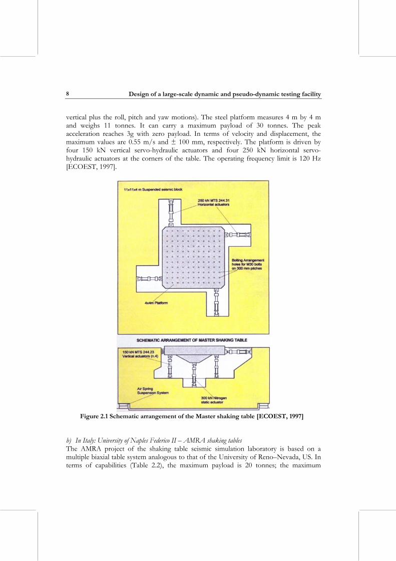
vertical plus the roll, pitch and yaw motions). The steel platform measures 4 m by 4 m and weighs 11 tonnes. It can carry a maximum payload of 30 tonnes. The peak acceleration reaches 3g with zero payload. In terms of velocity and displacement, the maximum values are 0.55 m/s and ± 100 mm, respectively. The platform is driven by four 150 kN vertical servo-hydraulic actuators and four 250 kN horizontal servo-hydraulic actuators at the corners of the table. The operating frequency limit is 120 Hz [ECOEST, 1997].
Figure 2.1 Schematic arrangement of the Master shaking table [ECOEST, 1997]
b) In Italy: University of Naples Federico II – AMRA shaking tables The AMRA project of the shaking table seismic simulation laboratory is based on a multiple biaxial table system analogous to that of the University of Reno–Nevada, US. In terms of capabilities (Table 2.2), the maximum payload is 20 tonnes; the maximum
Chapter 2: The new EUCENTRE facility
9
acceleration is 1g (with zero payload), the maximum velocity 1.0 m/s and the stroke ± 250 mm. The two shaking tables are 3 m by 3 m wide. The two tables can be set to produce a single biaxial table shaking in the two horizontal directions or to reproduce asynchronous seismic inputs through separate control of each table. In other words, they can be constrained to act together as a single large table or can be operated individually with independent motions [Fabbrocino and Cosenza, 2004]. c) In Italy: ENEA – Casaccia shaking tables In the earthquake-engineering laboratory of the ENEA-Casaccia, Rome, there are two shaking tables (Table 2.2). The first system is characterized by a platform with an overall size of 4 m by 4 m, a maximum payload of 10 tonnes, peak acceleration of 3g (with zero payload), peak velocity of 0.5 m/s and a stroke of ± 250 mm. The second shaking table is 2 m by 2 m wide and it has one tonne as maximum payload, 5g as peak acceleration for a bare table, 1.0 m/s as peak velocity and ± 300 mm stroke. Both systems have been designed as six degrees of freedom shaking tables. The testing frequency range is 0-50 Hz for the first system, and 0-100 Hz for the second one. d) In Europe: Centre for Studies and Equipment in Earthquake Engineering (Portugal) – 3D
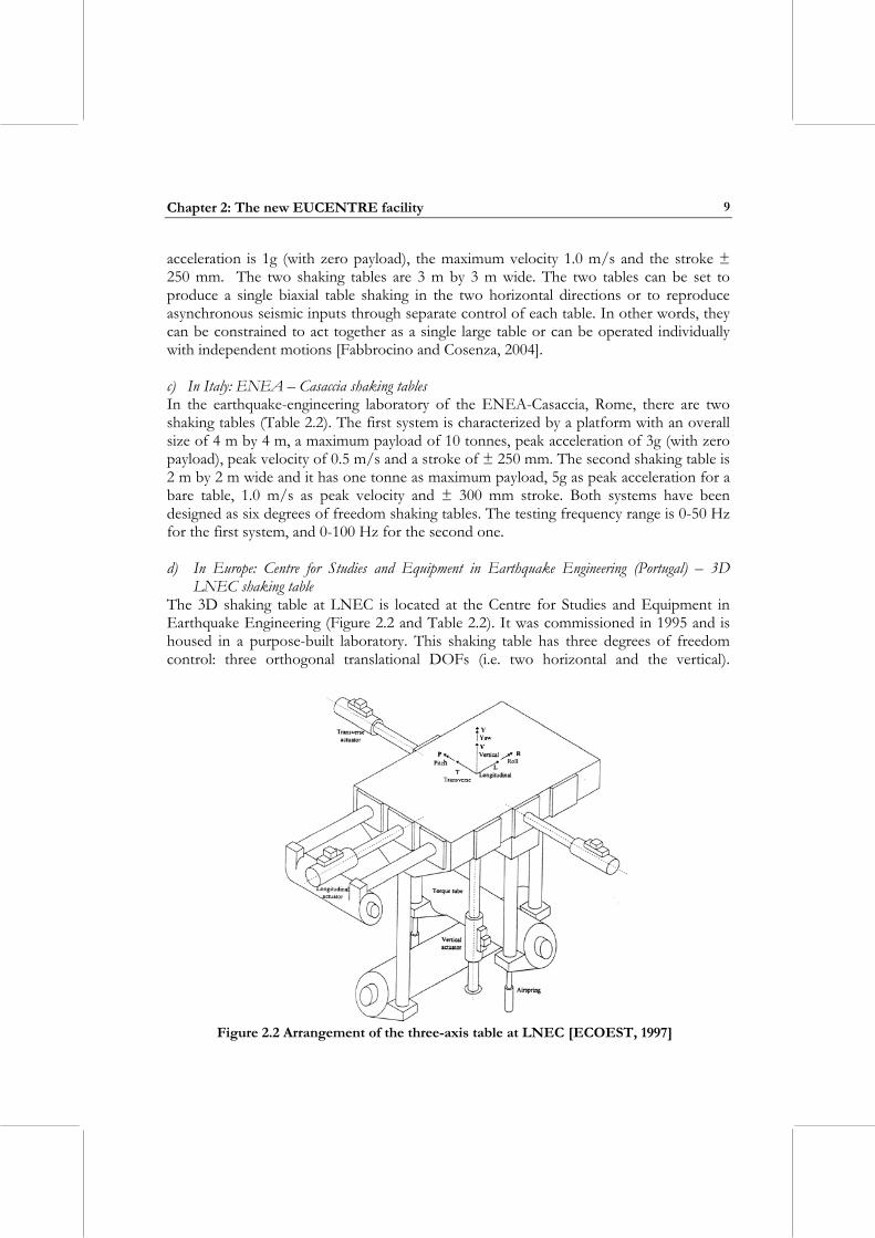
LNEC shaking table The 3D shaking table at LNEC is located at the Centre for Studies and Equipment in Earthquake Engineering (Figure 2.2 and Table 2.2). It was commissioned in 1995 and is housed in a purpose-built laboratory. This shaking table has three degrees of freedom control: three orthogonal translational DOFs (i.e. two horizontal and the vertical).
Figure 2.2 Arrangement of the three-axis table at LNEC [ECOEST, 1997]
Design of a large-scale dynamic and pseudo-dynamic testing facility
10
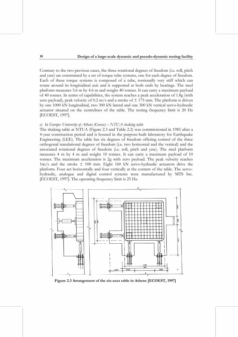
Contrary to the two previous cases, the three rotational degrees of freedom (i.e. roll, pitch and yaw) are constrained by a set of torque tube systems, one for each degree of freedom. Each of these torque systems is composed of a tube, torsionally very stiff which can rotate around its longitudinal axis and is supported at both ends by bearings. The steel platform measures 5.6 m by 4.6 m and weighs 40 tonnes. It can carry a maximum payload of 40 tonnes. In terms of capabilities, the system reaches a peak acceleration of 1.8g (with zero payload), peak velocity of 0.2 m/s and a stroke of ± 175 mm. The platform is driven by one 1000 kN longitudinal, two 300 kN lateral and one 300 kN vertical servo-hydraulic actuator situated on the centrelines of the table. The testing frequency limit is 20 Hz [ECOEST, 1997]. e) In Europe: University of Athens (Greece) – NTUA shaking table The shaking table at NTUA (Figure 2.3 and Table 2.2) was commissioned in 1985 after a 4-year construction period and is housed in the purpose-built laboratory for Earthquake Engineering (LEE). The table has six degrees of freedom offering control of the three orthogonal translational degrees of freedom (i.e. two horizontal and the vertical) and the associated rotational degrees of freedom (i.e. roll, pitch and yaw). The steel platform measures 4 m by 4 m and weighs 10 tonnes. It can carry a maximum payload of 10 tonnes. The maximum acceleration is 2g with zero payload. The peak velocity reaches 1m/s and the stroke ± 100 mm. Eight 160 kN servo-hydraulic actuators drive the platform. Four act horizontally and four vertically at the corners of the table. The servo-hydraulic, analogue and digital control systems were manufactured by MTS Inc. [ECOEST, 1997]. The operating frequency limit is 25 Hz.
Figure 2.3 Arrangement of the six-axes table in Athens [ECOEST, 1997]
Chapter 2: The new EUCENTRE facility
11
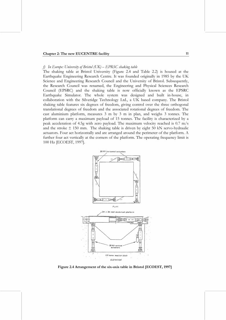
f) In Europe: University of Bristol (UK) – EPRSC shaking table The shaking table at Bristol University (Figure 2.4 and Table 2.2) is housed at the Earthquake Engineering Research Centre. It was founded originally in 1985 by the UK Science and Engineering Research Council and the University of Bristol. Subsequently, the Research Council was renamed, the Engineering and Physical Sciences Research Council (EPSRC) and the shaking table is now officially known as the EPSRC Earthquake Simulator. The whole system was designed and built in-house, in collaboration with the Silveridge Technology Ltd., a UK based company. The Bristol shaking table features six degrees of freedom, giving control over the three orthogonal translational degrees of freedom and the associated rotational degrees of freedom. The cast aluminium platform, measures 3 m by 3 m in plan, and weighs 3 tonnes. The platform can carry a maximum payload of 15 tonnes. The facility is characterized by a peak acceleration of 4.5g with zero payload. The maximum velocity reached is 0.7 m/s and the stroke ± 150 mm. The shaking table is driven by eight 50 kN servo-hydraulic actuators. Four act horizontally and are arranged around the perimeter of the platform. A further four act vertically at the corners of the platform. The operating frequency limit is 100 Hz [ECOEST, 1997].
Figure 2.4 Arrangement of the six-axis table in Bristol [ECOEST, 1997]
Design of a large-scale dynamic and pseudo-dynamic testing facility
12
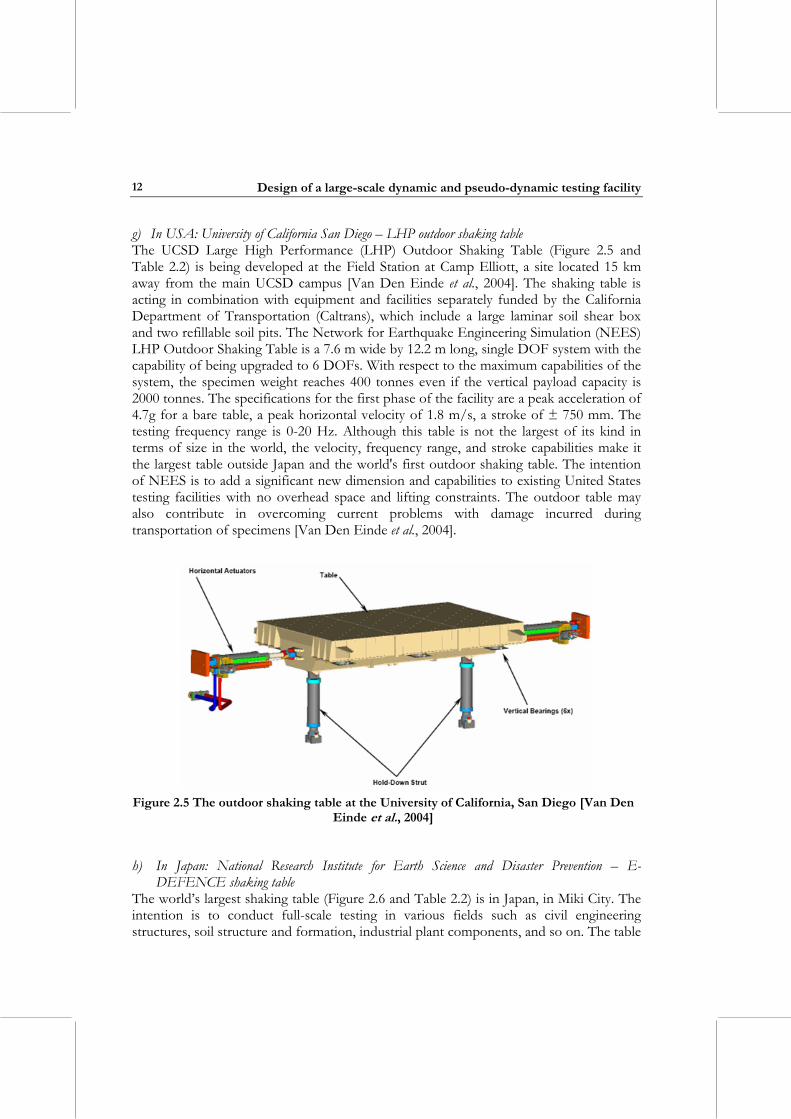
g) In USA: University of California San Diego – LHP outdoor shaking table The UCSD Large High Performance (LHP) Outdoor Shaking Table (Figure 2.5 and Table 2.2) is being developed at the Field Station at Camp Elliott, a site located 15 km away from the main UCSD campus [Van Den Einde et al., 2004]. The shaking table is acting in combination with equipment and facilities separately funded by the California Department of Transportation (Caltrans), which include a large laminar soil shear box and two refillable soil pits. The Network for Earthquake Engineering Simulation (NEES) LHP Outdoor Shaking Table is a 7.6 m wide by 12.2 m long, single DOF system with the capability of being upgraded to 6 DOFs. With respect to the maximum capabilities of the system, the specimen weight reaches 400 tonnes even if the vertical payload capacity is 2000 tonnes. The specifications for the first phase of the facility are a peak acceleration of 4.7g for a bare table, a peak horizontal velocity of 1.8 m/s, a stroke of ± 750 mm. The testing frequency range is 0-20 Hz. Although this table is not the largest of its kind in terms of size in the world, the velocity, frequency range, and stroke capabilities make it the largest table outside Japan and the world's first outdoor shaking table. The intention of NEES is to add a significant new dimension and capabilities to existing United States testing facilities with no overhead space and lifting constraints. The outdoor table may also contribute in overcoming current problems with damage incurred during transportation of specimens [Van Den Einde et al., 2004].
Figure 2.5 The outdoor shaking table at the University of California, San Diego [Van Den
Einde et al., 2004]
h) In Japan: National Research Institute for Earth Science and Disaster Prevention – E-
DEFENCE shaking table The world’s largest shaking table (Figure 2.6 and Table 2.2) is in Japan, in Miki City. The intention is to conduct full-scale testing in various fields such as civil engineering structures, soil structure and formation, industrial plant components, and so on. The table
Chapter 2: The new EUCENTRE facility
13
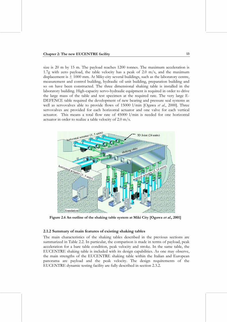
size is 20 m by 15 m. The payload reaches 1200 tonnes. The maximum acceleration is 1.7g with zero payload, the table velocity has a peak of 2.0 m/s, and the maximum displacement is ± 1000 mm. At Miky-city several buildings, such as the laboratory centre, measurement and control building, hydraulic oil unit building, preparation building and so on have been constructed. The three dimensional shaking table is installed in the laboratory building. High-capacity servo-hydraulic equipment is required in order to drive the large mass of the table and test specimen at the required rate. The very large E-DEFENCE table required the development of new bearing and pressure seal systems as well as servovalves able to provide flows of 15000 l/min [Ogawa et al., 2000]. Three servovalves are provided for each horizontal actuator and one valve for each vertical actuator. This means a total flow rate of 45000 l/min is needed for one horizontal actuator in order to realize a table velocity of 2.0 m/s.
Figure 2.6 An outline of the shaking table system at Miki City [Ogawa et al., 2001]
2.1.2 Summary of main features of existing shaking tables The main characteristics of the shaking tables described in the previous sections are summarized in Table 2.2. In particular, the comparison is made in terms of payload, peak acceleration for a bare table condition, peak velocity and stroke. In the same table, the EUCENTRE shaking table is included with its design capabilities. As one may observe, the main strengths of the EUCENTRE shaking table within the Italian and European panorama are payload and the peak velocity. The design requirements of the EUCENTRE dynamic testing facility are fully described in section 2.3.2.
Design of a large-scale dynamic and pseudo-dynamic testing facility
14
Table 2.2 Performance characteristics of the shaking tables reviewed above
Institution Payload [tonnes]
Peak acc. [g] *
Peak vel.
[m/s]
Stroke ±
[mm] NIED (Japan) 1200.00 1.7 2.00 1000 University of California San Diego (USA) 400.00 4.7 1.80 750 Centre for Studies & Equipment Earth. Eng. (Portugal) 40.00 1.8 0.20 175 CESI-ISMES (Italy) 30.00 3.0 0.55 100 University of Naples Federico II (Italy) 20.00 1.0 1.00 250 University of Bristol (UK) 15.00 4.5 0.70 150 ENEA (Italy) 10.00 3.0 1.00 250 University of Athens (Greece) 10.00 2.0 1.00 100 EUCENTRE (Italy) 60.00 5.0 1.50 500
* For a bare table condition
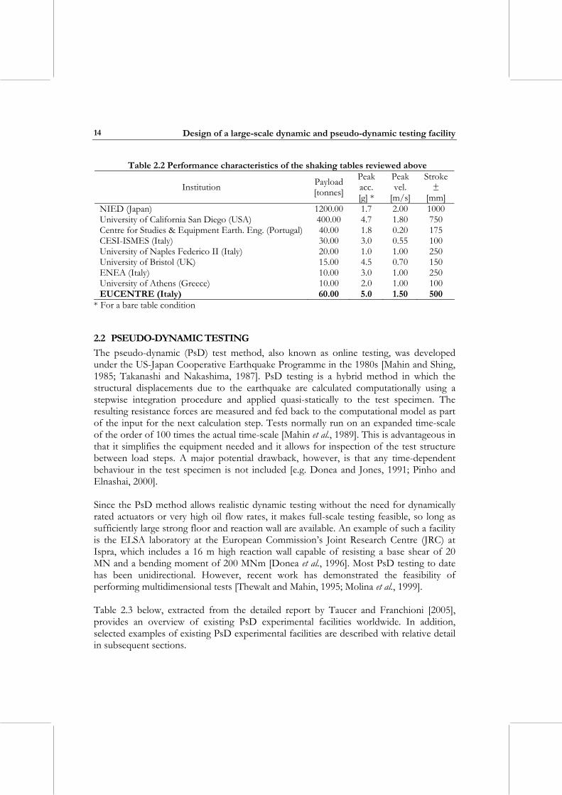
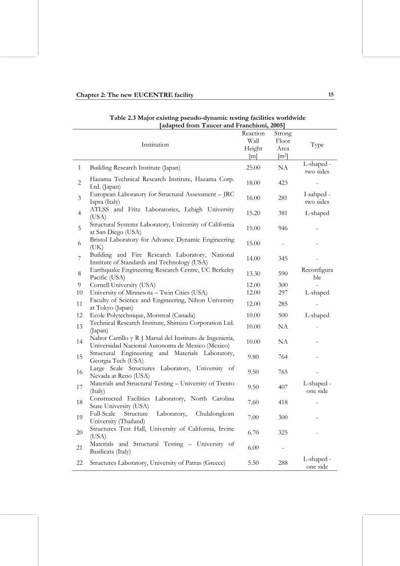
2.2 PSEUDO-DYNAMIC TESTING The pseudo-dynamic (PsD) test method, also known as online testing, was developed under the US-Japan Cooperative Earthquake Programme in the 1980s [Mahin and Shing, 1985; Takanashi and Nakashima, 1987]. PsD testing is a hybrid method in which the structural displacements due to the earthquake are calculated computationally using a stepwise integration procedure and applied quasi-statically to the test specimen. The resulting resistance forces are measured and fed back to the computational model as part of the input for the next calculation step. Tests normally run on an expanded time-scale of the order of 100 times the actual time-scale [Mahin et al., 1989]. This is advantageous in that it simplifies the equipment needed and it allows for inspection of the test structure between load steps. A major potential drawback, however, is that any time-dependent behaviour in the test specimen is not included [e.g. Donea and Jones, 1991; Pinho and Elnashai, 2000]. Since the PsD method allows realistic dynamic testing without the need for dynamically rated actuators or very high oil flow rates, it makes full-scale testing feasible, so long as sufficiently large strong floor and reaction wall are available. An example of such a facility is the ELSA laboratory at the European Commission’s Joint Research Centre (JRC) at Ispra, which includes a 16 m high reaction wall capable of resisting a base shear of 20 MN and a bending moment of 200 MNm [Donea et al., 1996]. Most PsD testing to date has been unidirectional. However, recent work has demonstrated the feasibility of performing multidimensional tests [Thewalt and Mahin, 1995; Molina et al., 1999]. Table 2.3 below, extracted from the detailed report by Taucer and Franchioni [2005], provides an overview of existing PsD experimental facilities worldwide. In addition, selected examples of existing PsD experimental facilities are described with relative detail in subsequent sections.
Chapter 2: The new EUCENTRE facility
15
Table 2.3 Major existing pseudo-dynamic testing facilities worldwide [adapted from Taucer and Franchioni, 2005]
Institution
Reaction Wall
Height [m]
Strong Floor Area [m2]
Type
1 Building Research Institute (Japan) 25.00 NA L-shaped - two sides
2 Hazama Technical Research Institute, Hazama Corp. Ltd. (Japan) 18.00 423 -
3 European Laboratory for Structural Assessment – JRC Ispra (Italy) 16.00 281 I-sahped -
two sides
4 ATLSS and Fritz Laboratories, Lehigh University (USA) 15.20 381 L-shaped
5 Structural Systems Laboratory, University of California at San Diego (USA) 15.00 946 -
6 Bristol Laboratory for Advance Dynamic Engineering (UK) 15.00 - -
7 Building and Fire Research Laboratory, National Institute of Standards and Technology (USA) 14.00 345 -
8 Earthquake Engineering Research Centre, UC Berkeley Pacific (USA) 13.30 590 Reconfigura
ble 9 Cornell University (USA) 12.00 300 - 10 University of Minnesota – Twin Cities (USA) 12.00 297 L-shaped
11 Faculty of Science and Engineering, Nihon University at Tokyo (Japan) 12.00 285 -
12 Ecole Polytechnique, Montreal (Canada) 10.00 500 L-shaped
13 Technical Research Institute, Shimizu Corporation Ltd. (Japan) 10.00 NA -
14 Nabor Carrillo y R J Marsal del Instituto de Ingenieria, Universidad Nacional Autonoma de Mexico (Mexico) 10.00 NA -
15 Structural Engineering and Materials Laboratory, Georgia Tech (USA) 9.80 764 -
16 Large Scale Structures Laboratory, University of Nevada at Reno (USA) 9.50 765 -
17 Materials and Structural Testing – University of Trento (Italy) 9.50 407 L-shaped -
one side
18 Constructed Facilities Laboratory, North Carolina State University (USA) 7.60 418 -
19 Full-Scale Structure Laboratory, Chulalongkom University (Thailand) 7.00 300 -
20 Structures Test Hall, University of California, Irvine (USA) 6.70 325 -
21 Materials and Structural Testing – University of Basilicata (Italy) 6.00 -
22 Structures Laboratory, University of Patras (Greece) 5.50 288 L-shaped - one side
Design of a large-scale dynamic and pseudo-dynamic testing facility
16
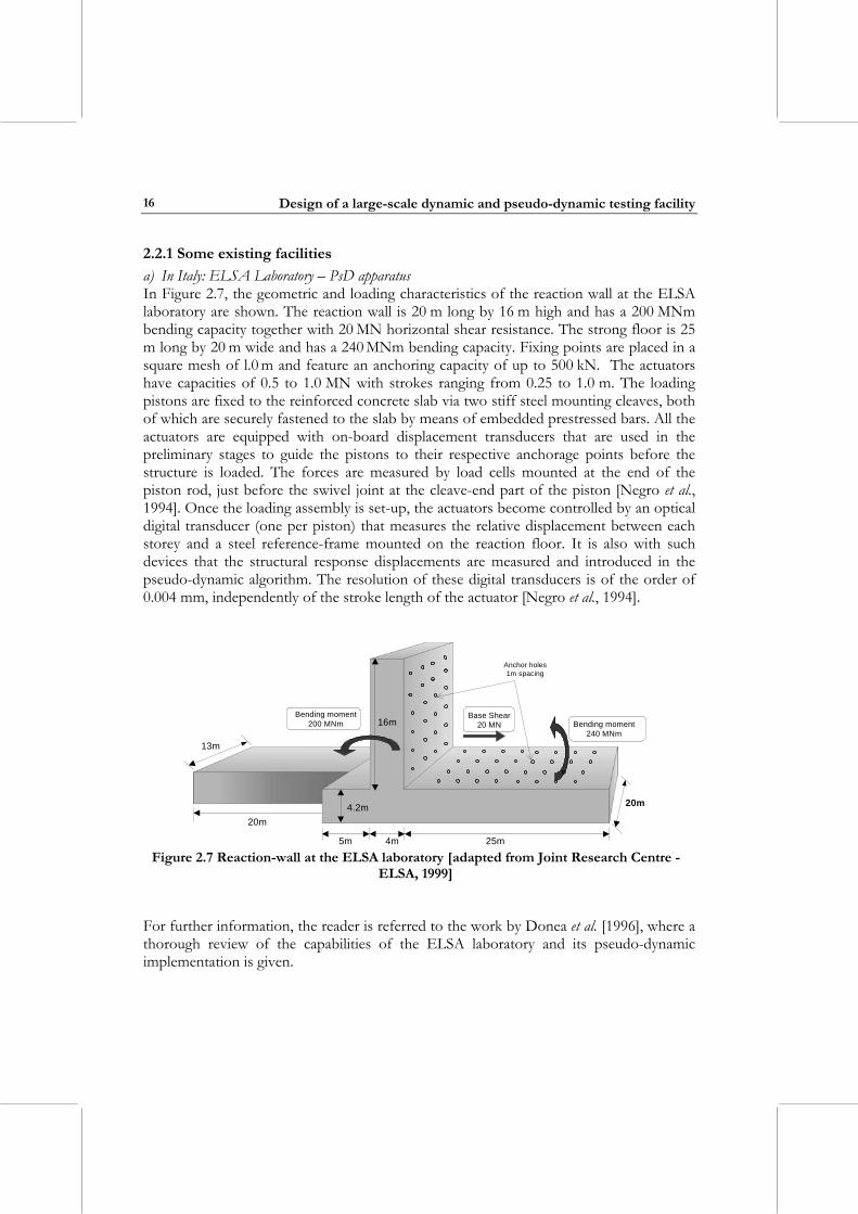
2.2.1 Some existing facilities a) In Italy: ELSA Laboratory – PsD apparatus In Figure 2.7, the geometric and loading characteristics of the reaction wall at the ELSA laboratory are shown. The reaction wall is 20 m long by 16 m high and has a 200 MNm bending capacity together with 20 MN horizontal shear resistance. The strong floor is 25 m long by 20 m wide and has a 240 MNm bending capacity. Fixing points are placed in a square mesh of l.0 m and feature an anchoring capacity of up to 500 kN. The actuators have capacities of 0.5 to 1.0 MN with strokes ranging from 0.25 to 1.0 m. The loading pistons are fixed to the reinforced concrete slab via two stiff steel mounting cleaves, both of which are securely fastened to the slab by means of embedded prestressed bars. All the actuators are equipped with on-board displacement transducers that are used in the preliminary stages to guide the pistons to their respective anchorage points before the structure is loaded. The forces are measured by load cells mounted at the end of the piston rod, just before the swivel joint at the cleave-end part of the piston [Negro et al., 1994]. Once the loading assembly is set-up, the actuators become controlled by an optical digital transducer (one per piston) that measures the relative displacement between each storey and a steel reference-frame mounted on the reaction floor. It is also with such devices that the structural response displacements are measured and introduced in the pseudo-dynamic algorithm. The resolution of these digital transducers is of the order of 0.004 mm, independently of the stroke length of the actuator [Negro et al., 1994].
16m
4.2m
25m4m5m
20m
13m
20m
Bending moment200 MNm Bending moment
240 MNm
Base Shear20 MN
Anchor holes1m spacing
Figure 2.7 Reaction-wall at the ELSA laboratory [adapted from Joint Research Centre -
ELSA, 1999]
For further information, the reader is referred to the work by Donea et al. [1996], where a thorough review of the capabilities of the ELSA laboratory and its pseudo-dynamic implementation is given.
Chapter 2: The new EUCENTRE facility
17
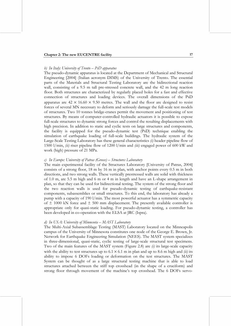
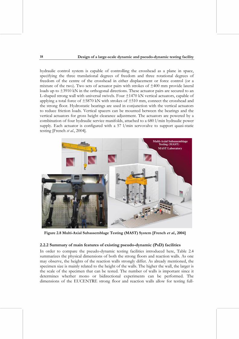
b) In Italy: University of Trento – PsD apparatus The pseudo-dynamic apparatus is located at the Department of Mechanical and Structural Engineering [2004] (Italian acronym DIMS) of the University of Trento. The essential parts of the Materials and Structural Testing Laboratory are the bidirectional reaction wall, consisting of a 9.5 m tall pre-stressed concrete wall, and the 42 m long reaction floor. Both structures are characterized by regularly placed holes for a fast and effective connection of structures and loading devices. The overall dimensions of the PsD apparatus are 42 × 16.60 × 9.50 metres. The wall and the floor are designed to resist forces of several MN necessary to deform and seriously damage the full-scale test models of structures. Two 10 tonnes bridge-cranes permit the movement and positioning of test structures. By means of computer-controlled hydraulic actuators it is possible to expose full-scale structures to dynamic strong forces and control the resulting displacements with high precision. In addition to static and cyclic tests on large structures and components, the facility is equipped for the pseudo-dynamic test (PsD) technique enabling the simulation of earthquake loading of full-scale buildings. The hydraulic system of the Large-Scale Testing Laboratory has these general characteristics (i) header pipeline flow of 1500 l/min, (ii) riser pipeline flow of 1200 l/min and (iii) engaged power of 600 kW and work (high) pressure of 21 MPa. c) In Europe: University of Patras (Greece) – Structures Laboratory The main experimental facility of the Structures Laboratory [University of Patras, 2004] consists of a strong floor, 18 m by 16 m in plan, with anchor points every 0.5 m in both directions, and two strong walls. These vertically prestressed walls are solid with thickness of 1.0 m, are 5.5 m high and 6 m or 4 m in length and have an L-shape arrangement in plan, so that they can be used for bidirectional testing. The system of the strong floor and the two reaction walls is used for pseudo-dynamic testing of earthquake-resistant components, subassemblies or small structures. To this end, the laboratory has already a pump with a capacity of 190 l/min. The most powerful actuator has a symmetric capacity of ± 1000 kN force and ± 500 mm displacement. The presently available controller is appropriate only for quasi-static loading. For pseudo-dynamic testing, a controller has been developed in co-operation with the ELSA at JRC (Ispra). d) In USA: University of Minnesota – MAST Laboratory The Multi-Axial Subassemblage Testing (MAST) Laboratory located on the Minneapolis campus of the University of Minnesota constitutes one node of the George E. Brown, Jr. Network for Earthquake Engineering Simulation (NEES). The MAST system specializes in three-dimensional, quasi-static, cyclic testing of large-scale structural test specimens. Two of the main features of the MAST system (Figure 2.8) are (i) its large-scale capacity with the ability to test structures up to 6.1 × 6.1 m in plan and up to 8.6 m high and (ii) its ability to impose 6 DOFs loading or deformation on the test structures. The MAST System can be thought of as a large structural testing machine that is able to load structures attached between the stiff top crosshead (in the shape of a cruciform) and strong floor through movement of the machine’s top crosshead. The 6 DOFs servo-
Design of a large-scale dynamic and pseudo-dynamic testing facility
18
hydraulic control system is capable of controlling the crosshead as a plane in space, specifying the three translational degrees of freedom and three rotational degrees of freedom of the centre of the crosshead in either displacement or force control (or a mixture of the two). Two sets of actuator pairs with strokes of ±400 mm provide lateral loads up to ±3910 kN in the orthogonal directions. These actuator pairs are secured to an L-shaped strong wall with universal swivels. Four ±1470 kN vertical actuators, capable of applying a total force of ±5870 kN with strokes of ±510 mm, connect the crosshead and the strong floor. Hydrostatic bearings are used in conjunction with the vertical actuators to reduce friction loads. Vertical spacers can be mounted between the bearings and the vertical actuators for gross height clearance adjustment. The actuators are powered by a combination of four hydraulic service manifolds, attached to a 680 l/min hydraulic power supply. Each actuator is configured with a 57 l/min servovalve to support quasi-static testing [French et al., 2004].
Figure 2.8 Multi-Axial Subassemblage Testing (MAST) System [French et al., 2004]
2.2.2 Summary of main features of existing pseudo-dynamic (PsD) facilities In order to compare the pseudo-dynamic testing facilities introduced here, Table 2.4 summarizes the physical dimensions of both the strong floors and reaction walls. As one may observe, the heights of the reaction walls strongly differ. As already mentioned, the specimen size is mainly related to the height of the walls. The higher the wall, the larger is the scale of the specimen that can be tested. The number of walls is important since it determines whether mono or bidirectional experiments can be performed. The dimensions of the EUCENTRE strong floor and reaction walls allow for testing full-
Chapter 2: The new EUCENTRE facility
19
scaled structures. The design requirements of the EUCENTRE pseudo-dynamic testing facility are fully described in section 2.3.3.
Table 2.4 Performance characteristics of the PsD facilities reviewed above
Institution Strong floor size [m]
Reaction wall height [m]
No. of walls
ELSA Laboratory (Italy) 25.00 × 20.00 16.0 1 University of Trento (Italy) 42.00 × 16.60 9.5 2 MAST (USA) 6.10 × 6.10 8.6 2 University of Patras (Greece) 6.00 × 4.00 5.5 1 EUCENTRE (Italy) 14.40 × 9.60 12.0 2
2.3 DEFINITION OF THE NEW EUCENTRE TESTING FACILITY PERFORMANCE TARGETS
2.3.1 Local needs and constraints When a dynamic and pseudo-dynamic testing facility is designed, the main goal is to develop a laboratory that provides the possibility of performing experimental tests on structures without limitations in terms of capacity. For example, the specifications of a shaking table should define a facility capable of simulating the mechanisms of collapse of structures under strong earthquake motions. To simulate real three-dimensional earthquake motion the first requirement is the number of allowed degrees of freedom (DOFs) of the shaking tables. They must at least be three. Secondly, the size of ground motion that can be reproduced is normally governed by its velocity content. This is directly related to the oil flow rate that can be provided by the pumping system and servovalves. To test real full-scale structures the size of the platform has to be large enough to support multi-stories buildings. The majority of test structures have a rectangular shape, e.g. buildings, bridges, soil boxes and pipelines. In order to use the table area effectively under the test weight limit, a rectangular-shaped table is desirable in most vibrational tests. In order to verify failure mechanisms and to develop effective isolation systems for real structures, the largest possible test models of the correct shape are desirable though technical and economic conditions must be taken into account. To design a large table the required technological know-how and cost must be accurately taken into account since ad-hoc devices (i.e. actuators, servovalves) have to be designed and fabricated. Each proposed test project must be financially supported. Apart from the construction costs, the manufacturing, assembling and installing of actuators, oil-pressure supply system and other major parts of dynamic and pseudo-dynamic facility, heavily contribute to the choice of design specifications.
Design of a large-scale dynamic and pseudo-dynamic testing facility
20
The current worldwide design trend is to build facilities whose velocity and displacement performance limits are emphasized more than acceleration. The world’s largest and powerful shaking table has been developed in Japan. The construction of the facility (named E-Defence) at Miki-city (see section 2.1.1b) started in 1998, the research and development for core technology were started in 1995 and the entire work has been completed in the beginning of 2005. The implied extensive research and development work was possible through a close cooperation of dozens of a number of research centres, universities, independent administrative institutions and private companies. The new outdoor shaking table in San Diego (see section 2.1.1g), on the other hand, was designed to be the world’s first outdoor shaking table adding a significant new dimension and capabilities to existing USA testing facility with no overhead space and lifting constraints. The NEES/LHP Outdoor Shaking Table in San Diego is a single DOF system with the capability of upgrading to 6 DOFs. The new testing facility at the European Centre for Training and Research in Earthquake Engineering (EUCENTRE), features within the same laboratory a dynamic and a pseudo-dynamic testing facility. This choice is justified by the performance limitations of the shaking table, which, as described below, do not allow for dynamic tests on real full-scaled structures such as three or four-storey buildings. For such structures, the neighbouring PsD apparatus can be employed, without significant limitations. The design of the table follows the Japanese trend of high velocity and large amplitude requirements in order to reproduce the size of real earthquakes. The shape of the table is rectangular like the Miki City large table and the NEES/LHP Outdoor Shaking Table in San Diego. Moreover, and perhaps more importantly, the characteristics of this new testing facility have been chosen so as to complement, rather than to compete, with existing earthquake engineering testing facilities in Europe, and, in particular, in Italy, summarised in previous sections of this chapter. Open cooperation with Reluis, the Italian National Network of Earthquake Engineering University Laboratories, eased the attainment of such important objective.
2.3.2 General description of the EUCENTRE dynamic testing facility requirements
The importance of promoting strengthening and rationalization of earthquake-proof structural design is one of the lessons from the most recent earthquakes. Since earthquake vibrations involve three-dimensional movement of the structure, it should be ideal to set up a three-dimensional earthquake simulator facility to accurately reproduce earthquake ground motions. For the EUCENTRE shaking table, priority was given to size and power rather than DOF in order to perform tests on full-scale or large-scale models of test structures and foundations. Therefore, a large, powerful, one-dimensional platform was chosen with respect to a small six DOF table with limited performance capabilities (Table 2.2). Single-axis shaking tables are the simplest form of table. For many
Chapter 2: The new EUCENTRE facility
21
tests it is only desirable to excite the specimen in one axis as this simplifies subsequent interpretation of the results. In these cases, single-axis tables may provide the best solution for performing the test if they have a large enough dynamic capacity. Single-axis tables are also slightly simpler to control than multi-axis tables. The main disadvantage of single-axis tables is their inability to investigate the more complex behaviour of structures under loading in more than one axis. Like the Miki City large table and the LHP Outdoor shaking table (section 2.1.1), the EUCENTRE platform has a rectangular shape (see section 2.3.1). The dimensions in plan are 7.0 m by 5.6 m as described in section 3.2.1. The size of the platform automatically constrains the dimensions of the test specimen, be it reinforced concrete and/or masonry buildings, shear walls, retaining walls, bridge piers, and so on. A compromise is often required between the capabilities and the platform dimensions. The capacity to accurately reproduce near-fault ground motion effects was considered essential for the EUCENTRE facility since, the seismic hazard of the built environment is controlled by near-field ground motion at long return period hazard (e.g. 2% probability of exceedence in 50 years) for many sites. Near-field, fault normal, ground motion records with forward directivity effects (Doppler effects) are characterized by a large velocity pulse, while near-field, fault parallel, ground motion records are characterized by a fling step (i.e., large step function in the ground displacement record). This is controlled by the peak table velocity parameter. A peak table velocity of 1.5 m/s was selected according to the available near-fault seismological data and as a compromise between technical performance and budgetary constraints. For the reproduction of far-field ground motions, a maximum horizontal peak ground and peak table acceleration of 1.8g (with maximum payload, see section 5.2), corresponding to an upper bound of the vast majority of recorded ground motion records, was considered. The significant frequency content of actual earthquake horizontal ground acceleration records lies in the range between 0 to 15 Hz, while the significant frequency component of horizontal ground velocity and displacement records lie in a lower frequency range than that of the acceleration. A frequency bandwidth of 20 Hz for accurate reproduction of actual full-scale ground acceleration records by the table was chosen. With regard to the construction technology, a steel welded platform was chosen. The platform consists of a closed steel box structure constructed in a single piece. Several tables are made in steel or aluminium. The table could be made from several aluminium sections bolted and glued together. The platform surface could be an arrangement of aluminium plates or even magnesium plates. Since the table has to survive experiments without deformations, the stiffness of steel made it preferable compared to aluminium.
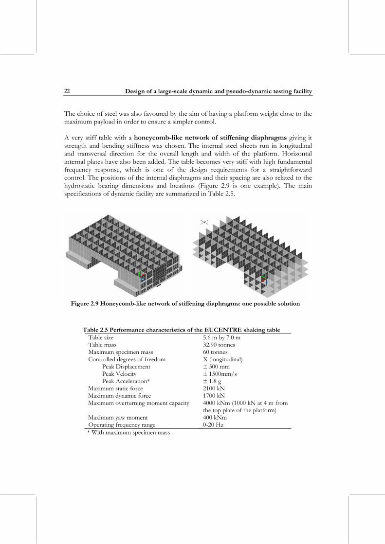
Design of a large-scale dynamic and pseudo-dynamic testing facility
22
The choice of steel was also favoured by the aim of having a platform weight close to the maximum payload in order to ensure a simpler control. A very stiff table with a honeycomb-like network of stiffening diaphragms giving it strength and bending stiffness was chosen. The internal steel sheets run in longitudinal and transversal direction for the overall length and width of the platform. Horizontal internal plates have also been added. The table becomes very stiff with high fundamental frequency response, which is one of the design requirements for a straightforward control. The positions of the internal diaphragms and their spacing are also related to the hydrostatic bearing dimensions and locations (Figure 2.9 is one example). The main specifications of dynamic facility are summarized in Table 2.5.
Figure 2.9 Honeycomb-like network of stiffening diaphragms: one possible solution
Table 2.5 Performance characteristics of the EUCENTRE shaking table
Table size 5.6 m by 7.0 m Table mass 32.90 tonnes Maximum specimen mass 60 tonnes Controlled degrees of freedom X (longitudinal)
Peak Displacement ± 500 mm Peak Velocity ± 1500mm/s Peak Acceleration* ± 1.8 g
Maximum static force 2100 kN Maximum dynamic force 1700 kN Maximum overturning moment capacity 4000 kNm (1000 kN at 4 m from
the top plate of the platform) Maximum yaw moment 400 kNm Operating frequency range 0-20 Hz * With maximum specimen mass
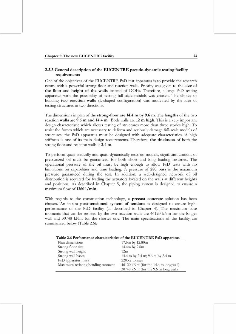
Chapter 2: The new EUCENTRE facility
23
2.3.3 General description of the EUCENTRE pseudo-dynamic testing facility requirements
One of the objectives of the EUCENTRE PsD test apparatus is to provide the research centre with a powerful strong floor and reaction walls. Priority was given to the size of the floor and height of the walls instead of DOFs. Therefore, a large PsD testing apparatus with the possibility of testing full-scale models was chosen. The choice of building two reaction walls (L-shaped configuration) was motivated by the idea of testing structures in two directions. The dimensions in plan of the strong-floor are 14.4 m by 9.6 m. The lengths of the two reaction walls are 9.6 m and 14.4 m. Both walls are 12 m high. This is a very important design characteristic which allows testing of structures more than three stories high. To resist the forces which are necessary to deform and seriously damage full-scale models of structures, the PsD apparatus must be designed with adequate characteristics. A high stiffness is one of its main design requirements. Therefore, the thickness of both the strong floor and reaction walls is 2.4 m. To perform quasi-statically and quasi-dynamically tests on models, significant amount of pressurized oil must be guaranteed for both short and long loading histories. The operational pressure of the oil must be high enough to allow PsD tests with no limitations on capabilities and time loading. A pressure of 280 bars is the maximum pressure guaranteed during the test. In addition, a well-designed network of oil distribution is required for feeding the actuators located on the walls at different heights and positions. As described in Chapter 5, the piping system is designed to ensure a maximum flow of 1360 l/min. With regards to the construction technology, a precast concrete solution has been chosen. An in-situ post-tensioned system of tendons is designed to ensure high-performance of the PsD facility (as described in Chapter 4). The maximum base moments that can be resisted by the two reaction walls are 46120 kNm for the longer wall and 30748 kNm for the shorter one. The main specifications of the facility are summarized below (Table 2.6):
Table 2.6 Performance characteristics of the EUCENTRE PsD apparatus Plan dimensions 17.6m by 12.80m Strong floor size 14.4m by 9.6m Strong wall height 12m Strong wall bases 14.4 m by 2.4 m; 9.6 m by 2.4 m PsD apparatus mass 2203.2 tonnes Maximum resisting bending moment 46120 kNm (for the 14.4 m long wall) 30748 kNm (for the 9.6 m long wall)

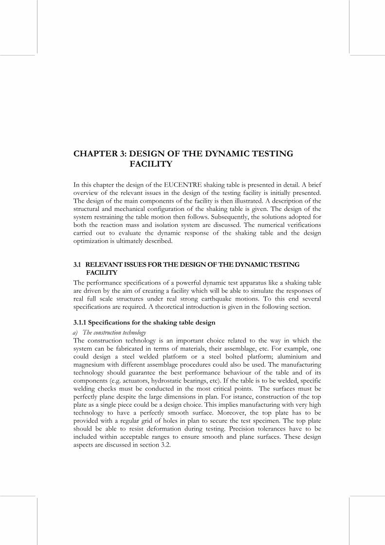
CHAPTER 3: DESIGN OF THE DYNAMIC TESTING FACILITY
In this chapter the design of the EUCENTRE shaking table is presented in detail. A brief overview of the relevant issues in the design of the testing facility is initially presented. The design of the main components of the facility is then illustrated. A description of the structural and mechanical configuration of the shaking table is given. The design of the system restraining the table motion then follows. Subsequently, the solutions adopted for both the reaction mass and isolation system are discussed. The numerical verifications carried out to evaluate the dynamic response of the shaking table and the design optimization is ultimately described.
3.1 RELEVANT ISSUES FOR THE DESIGN OF THE DYNAMIC TESTING FACILITY
The performance specifications of a powerful dynamic test apparatus like a shaking table are driven by the aim of creating a facility which will be able to simulate the responses of real full scale structures under real strong earthquake motions. To this end several specifications are required. A theoretical introduction is given in the following section.
3.1.1 Specifications for the shaking table design a) The construction technology The construction technology is an important choice related to the way in which the system can be fabricated in terms of materials, their assemblage, etc. For example, one could design a steel welded platform or a steel bolted platform; aluminium and magnesium with different assemblage procedures could also be used. The manufacturing technology should guarantee the best performance behaviour of the table and of its components (e.g. actuators, hydrostatic bearings, etc). If the table is to be welded, specific welding checks must be conducted in the most critical points. The surfaces must be perfectly plane despite the large dimensions in plan. For istance, construction of the top plate as a single piece could be a design choice. This implies manufacturing with very high technology to have a perfectly smooth surface. Moreover, the top plate has to be provided with a regular grid of holes in plan to secure the test specimen. The top plate should be able to resist deformation during testing. Precision tolerances have to be included within acceptable ranges to ensure smooth and plane surfaces. These design aspects are discussed in section 3.2.
Design of a large-scale dynamic and pseudo-dynamic testing facility
26
b) Materials The choice of construction material is limited by the specifications of the facility. If the table must be light, aluminium gives the possibility to create limited weight platforms. If the customer wants a heavy platform, steel is the most appropriate material with the possibility of adding concrete blocks within the table to reach the design weight. A very light platform has the advantage that it requires a smaller actuator to move it, which thereby reduces the initial cost of the facility. However, a very light platform is much more likely to be affected by significant table-specimen interaction which requires better hardware and software systems to effectively control. Therefore the larger the platform mass the better it is from the point of view of the specimen, but this requires larger actuators, increases running costs and can limit the maximum accelerations achievable. A solution of this conflict is the use of a light platform with high capacity actuators. For small light specimens the platform is used as it is, but when a larger specimen that may interact significantly with the table is to be tested, then additional static mass, up to the capacity of the table, may be added to the platform. This additional mass then helps to reduce the table-specimen interaction by increasing the platform mass that has to be excited by the specimen. The other effect of having a larger, more massive platform is simply the enhanced capacity of the shaking table to deal with larger scale models. The larger the model, the simpler the scaling issue becomes. Therefore, within the limits imposed by cost of construction of the shaking table, the running costs and the cost of manufacture of models, the largest mass of the platform and capacity of the table should be chosen (as described in section 3.2.). c) Shaking table stiffness The stiffness of the table and the bearings must be very high to reach frequency responses beyond the range of fundamental frequencies of the test structures. The design of a shaking table requires accurate considerations of the response frequencies of all the components of the facility since the resonance of the response can cause unforeseen amplifications of motions. The first frequency to take into account is the frequency related to the “oil-column” stiffness. A test system’s first natural mode of vibration usually depends on the platform/payload mass and its “oil-column” stiffness, i.e. the stiffness of the compressible oil in the actuators. This “oil-column” stiffness is important in all hydraulic systems as it usually defines the first resonant frequency. A system’s dynamic behaviour is quite different at excitation below and above this frequency. The oil’s effective bulk modulus of elasticity (or compressibility) depends on the oil’s material properties as well as factors such as entrained air; temperature and mechanical compliance (see section 5.2). Since the stiffness of a “column” of oil is inversely proportional to its length, a long-stroke actuator should have small oil-column stiffness. The overall dynamic system has a natural mode of vibration and frequency content dependent on the mobilized mass and the actuator stiffness. The platform should be sufficiently rigid in order not to respond itself dynamically so that it transmits the input motion to the structure with as little modification as possible (described in sections 3.2 and 3.3). In addition, there is the variation in motion across the table surface itself. The
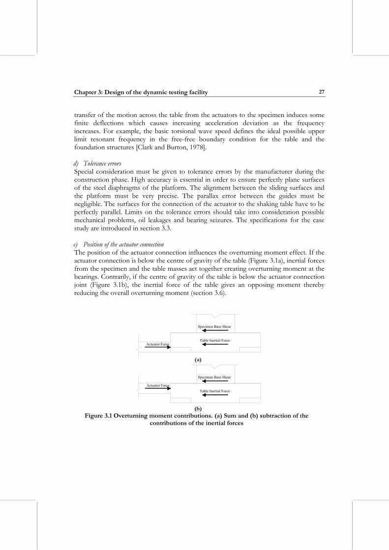
Chapter 3: Design of the dynamic testing facility
27
transfer of the motion across the table from the actuators to the specimen induces some finite deflections which causes increasing acceleration deviation as the frequency increases. For example, the basic torsional wave speed defines the ideal possible upper limit resonant frequency in the free-free boundary condition for the table and the foundation structures [Clark and Burton, 1978]. d) Tolerance errors Special consideration must be given to tolerance errors by the manufacturer during the construction phase. High accuracy is essential in order to ensure perfectly plane surfaces of the steel diaphragms of the platform. The alignment between the sliding surfaces and the platform must be very precise. The parallax error between the guides must be negligible. The surfaces for the connection of the actuator to the shaking table have to be perfectly parallel. Limits on the tolerance errors should take into consideration possible mechanical problems, oil leakages and bearing seizures. The specifications for the case study are introduced in section 3.3. e) Position of the actuator connection The position of the actuator connection influences the overturning moment effect. If the actuator connection is below the centre of gravity of the table (Figure 3.1a), inertial forces from the specimen and the table masses act together creating overturning moment at the bearings. Contrarily, if the centre of gravity of the table is below the actuator connection joint (Figure 3.1b), the inertial force of the table gives an opposing moment thereby reducing the overall overturning moment (section 3.6).
Specimen Base Shear
Table Inertial ForceActuator Force
(a)
Specimen Base Shear
Actuator ForceTable Inertial Force
(b)
Figure 3.1 Overturning moment contributions. (a) Sum and (b) subtraction of the contributions of the inertial forces
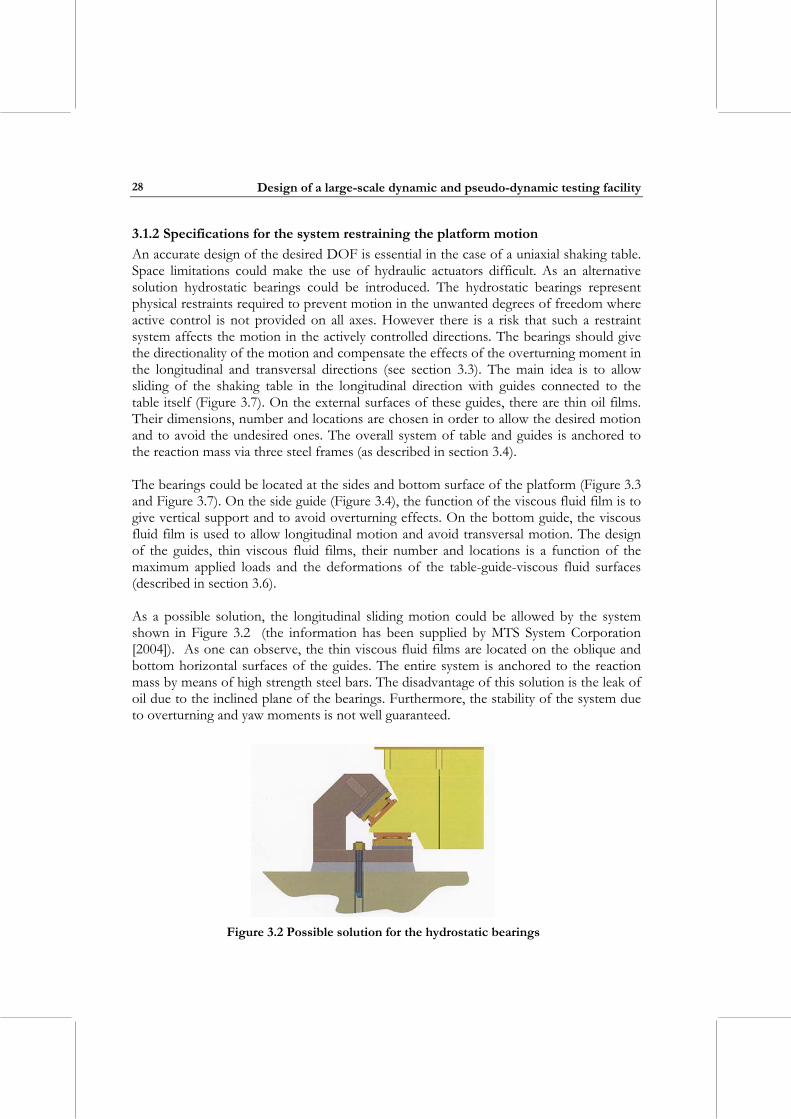
Design of a large-scale dynamic and pseudo-dynamic testing facility
28
3.1.2 Specifications for the system restraining the platform motion An accurate design of the desired DOF is essential in the case of a uniaxial shaking table. Space limitations could make the use of hydraulic actuators difficult. As an alternative solution hydrostatic bearings could be introduced. The hydrostatic bearings represent physical restraints required to prevent motion in the unwanted degrees of freedom where active control is not provided on all axes. However there is a risk that such a restraint system affects the motion in the actively controlled directions. The bearings should give the directionality of the motion and compensate the effects of the overturning moment in the longitudinal and transversal directions (see section 3.3). The main idea is to allow sliding of the shaking table in the longitudinal direction with guides connected to the table itself (Figure 3.7). On the external surfaces of these guides, there are thin oil films. Their dimensions, number and locations are chosen in order to allow the desired motion and to avoid the undesired ones. The overall system of table and guides is anchored to the reaction mass via three steel frames (as described in section 3.4). The bearings could be located at the sides and bottom surface of the platform (Figure 3.3 and Figure 3.7). On the side guide (Figure 3.4), the function of the viscous fluid film is to give vertical support and to avoid overturning effects. On the bottom guide, the viscous fluid film is used to allow longitudinal motion and avoid transversal motion. The design of the guides, thin viscous fluid films, their number and locations is a function of the maximum applied loads and the deformations of the table-guide-viscous fluid surfaces (described in section 3.6). As a possible solution, the longitudinal sliding motion could be allowed by the system shown in Figure 3.2 (the information has been supplied by MTS System Corporation [2004]). As one can observe, the thin viscous fluid films are located on the oblique and bottom horizontal surfaces of the guides. The entire system is anchored to the reaction mass by means of high strength steel bars. The disadvantage of this solution is the leak of oil due to the inclined plane of the bearings. Furthermore, the stability of the system due to overturning and yaw moments is not well guaranteed.
Figure 3.2 Possible solution for the hydrostatic bearings
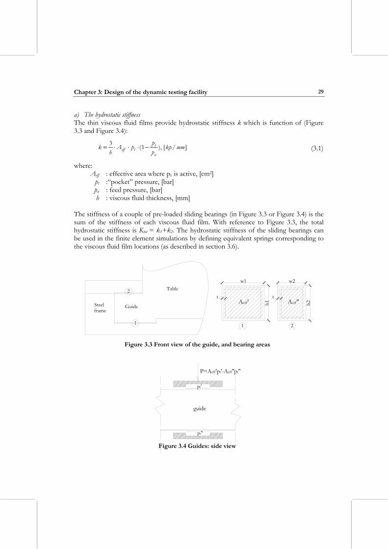
Chapter 3: Design of the dynamic testing facility
29
a) The hydrostatic stiffness The thin viscous fluid films provide hydrostatic stiffness k which is function of (Figure 3.3 and Figure 3.4):
]/[),1(3 mmkppp
pAh
ka
tteff −⋅⋅⋅= (3.1)
where: Aeff : effective area where pt is active, [cm2]
pt :“pocket” pressure, [bar] pa : feed pressure, [bar] h : viscous fluid thickness, [mm]
The stiffness of a couple of pre-loaded sliding bearings (in Figure 3.3 or Figure 3.4) is the sum of the stiffness of each viscous fluid film. With reference to Figure 3.3, the total hydrostatic stiffness is Ktot = k1+k2. The hydrostatic stiffness of the sliding bearings can be used in the finite element simulations by defining equivalent springs corresponding to the viscous fluid film locations (as described in section 3.6).
t t
w2
Aeff''
2
b2b1
w1
1
Aeff'
1
2 Table
GuideSteel frame
Figure 3.3 Front view of the guide, and bearing areas
pt'
pt''
P=Aeff'pt'-Aeff''pt''
guide
Figure 3.4 Guides: side view
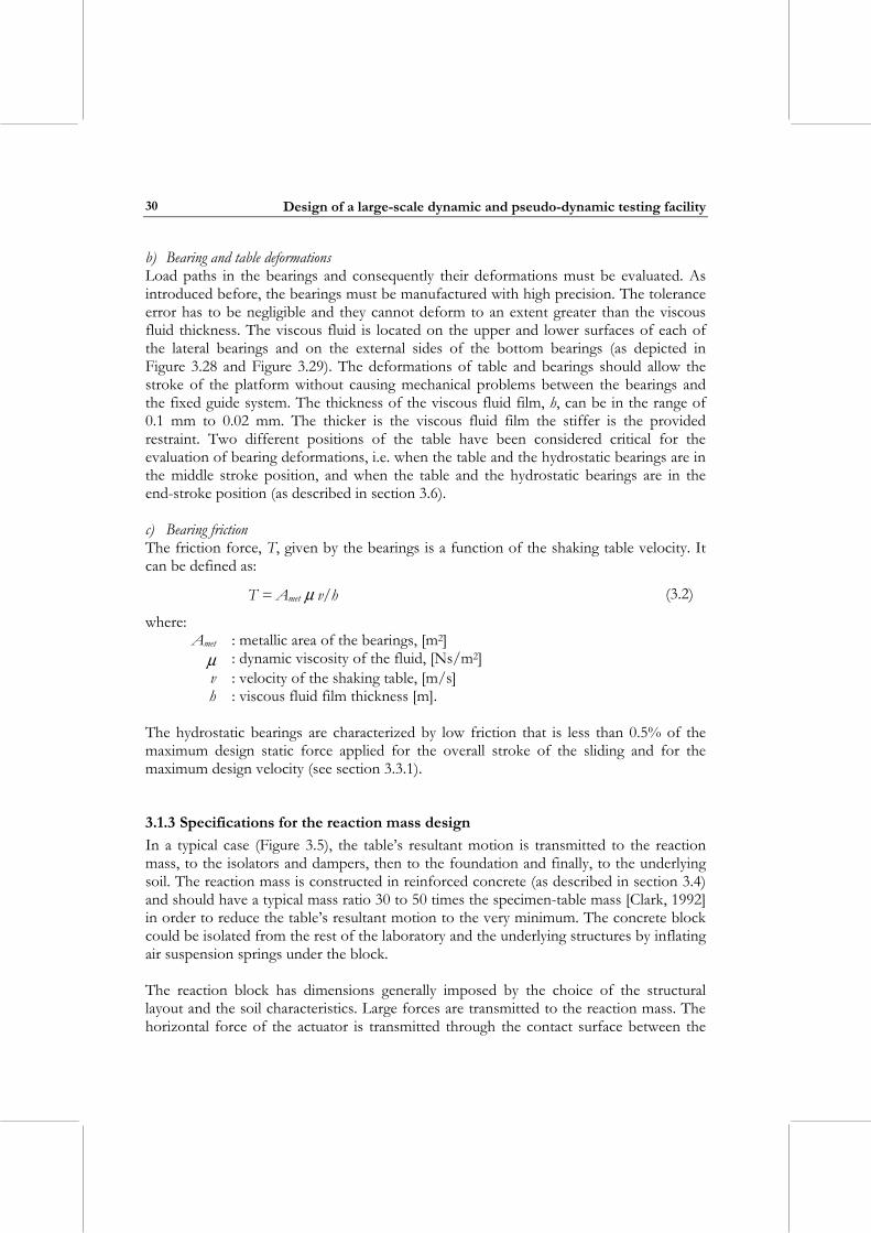
Design of a large-scale dynamic and pseudo-dynamic testing facility
30
b) Bearing and table deformations Load paths in the bearings and consequently their deformations must be evaluated. As introduced before, the bearings must be manufactured with high precision. The tolerance error has to be negligible and they cannot deform to an extent greater than the viscous fluid thickness. The viscous fluid is located on the upper and lower surfaces of each of the lateral bearings and on the external sides of the bottom bearings (as depicted in Figure 3.28 and Figure 3.29). The deformations of table and bearings should allow the stroke of the platform without causing mechanical problems between the bearings and the fixed guide system. The thickness of the viscous fluid film, h, can be in the range of 0.1 mm to 0.02 mm. The thicker is the viscous fluid film the stiffer is the provided restraint. Two different positions of the table have been considered critical for the evaluation of bearing deformations, i.e. when the table and the hydrostatic bearings are in the middle stroke position, and when the table and the hydrostatic bearings are in the end-stroke position (as described in section 3.6). c) Bearing friction The friction force, T, given by the bearings is a function of the shaking table velocity. It can be defined as:
T = Amet µ v/h (3.2)
where: Amet : metallic area of the bearings, [m2]
µ : dynamic viscosity of the fluid, [Ns/m2] v : velocity of the shaking table, [m/s] h : viscous fluid film thickness [m].
The hydrostatic bearings are characterized by low friction that is less than 0.5% of the maximum design static force applied for the overall stroke of the sliding and for the maximum design velocity (see section 3.3.1).
3.1.3 Specifications for the reaction mass design In a typical case (Figure 3.5), the table’s resultant motion is transmitted to the reaction mass, to the isolators and dampers, then to the foundation and finally, to the underlying soil. The reaction mass is constructed in reinforced concrete (as described in section 3.4) and should have a typical mass ratio 30 to 50 times the specimen-table mass [Clark, 1992] in order to reduce the table’s resultant motion to the very minimum. The concrete block could be isolated from the rest of the laboratory and the underlying structures by inflating air suspension springs under the block. The reaction block has dimensions generally imposed by the choice of the structural layout and the soil characteristics. Large forces are transmitted to the reaction mass. The horizontal force of the actuator is transmitted through the contact surface between the
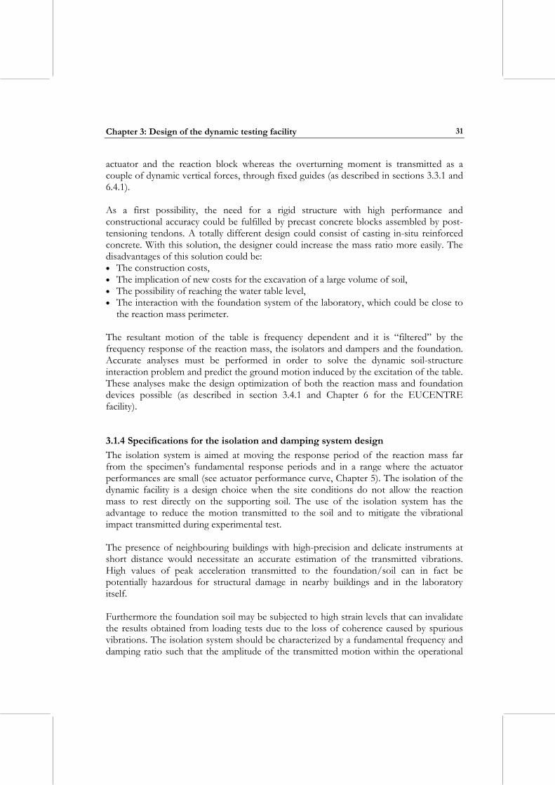
Chapter 3: Design of the dynamic testing facility
31
actuator and the reaction block whereas the overturning moment is transmitted as a couple of dynamic vertical forces, through fixed guides (as described in sections 3.3.1 and 6.4.1). As a first possibility, the need for a rigid structure with high performance and constructional accuracy could be fulfilled by precast concrete blocks assembled by post-tensioning tendons. A totally different design could consist of casting in-situ reinforced concrete. With this solution, the designer could increase the mass ratio more easily. The disadvantages of this solution could be: • The construction costs, • The implication of new costs for the excavation of a large volume of soil, • The possibility of reaching the water table level, • The interaction with the foundation system of the laboratory, which could be close to
the reaction mass perimeter. The resultant motion of the table is frequency dependent and it is “filtered” by the frequency response of the reaction mass, the isolators and dampers and the foundation. Accurate analyses must be performed in order to solve the dynamic soil-structure interaction problem and predict the ground motion induced by the excitation of the table. These analyses make the design optimization of both the reaction mass and foundation devices possible (as described in section 3.4.1 and Chapter 6 for the EUCENTRE facility).
3.1.4 Specifications for the isolation and damping system design The isolation system is aimed at moving the response period of the reaction mass far from the specimen’s fundamental response periods and in a range where the actuator performances are small (see actuator performance curve, Chapter 5). The isolation of the dynamic facility is a design choice when the site conditions do not allow the reaction mass to rest directly on the supporting soil. The use of the isolation system has the advantage to reduce the motion transmitted to the soil and to mitigate the vibrational impact transmitted during experimental test. The presence of neighbouring buildings with high-precision and delicate instruments at short distance would necessitate an accurate estimation of the transmitted vibrations. High values of peak acceleration transmitted to the foundation/soil can in fact be potentially hazardous for structural damage in nearby buildings and in the laboratory itself. Furthermore the foundation soil may be subjected to high strain levels that can invalidate the results obtained from loading tests due to the loss of coherence caused by spurious vibrations. The isolation system should be characterized by a fundamental frequency and damping ratio such that the amplitude of the transmitted motion within the operational
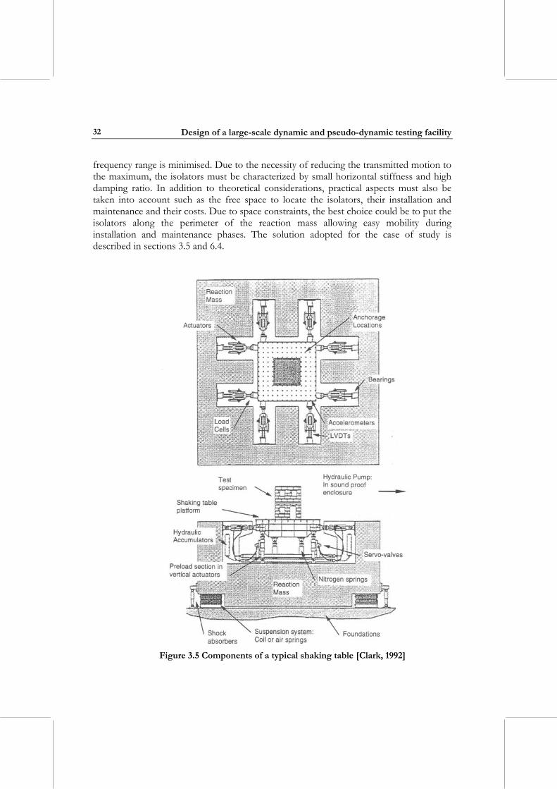
Design of a large-scale dynamic and pseudo-dynamic testing facility
32
frequency range is minimised. Due to the necessity of reducing the transmitted motion to the maximum, the isolators must be characterized by small horizontal stiffness and high damping ratio. In addition to theoretical considerations, practical aspects must also be taken into account such as the free space to locate the isolators, their installation and maintenance and their costs. Due to space constraints, the best choice could be to put the isolators along the perimeter of the reaction mass allowing easy mobility during installation and maintenance phases. The solution adopted for the case of study is described in sections 3.5 and 6.4.
Figure 3.5 Components of a typical shaking table [Clark, 1992]
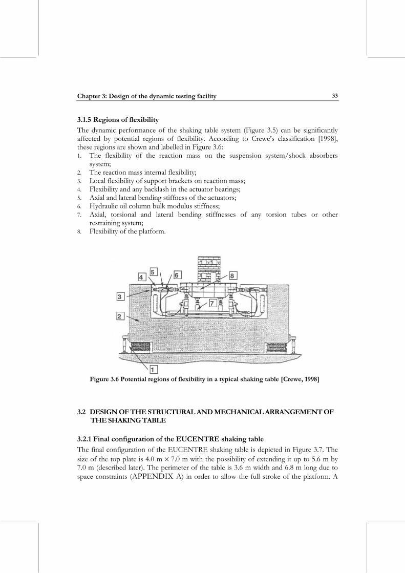
Chapter 3: Design of the dynamic testing facility
33
3.1.5 Regions of flexibility The dynamic performance of the shaking table system (Figure 3.5) can be significantly affected by potential regions of flexibility. According to Crewe’s classification [1998], these regions are shown and labelled in Figure 3.6: 1. The flexibility of the reaction mass on the suspension system/shock absorbers
system; 2. The reaction mass internal flexibility; 3. Local flexibility of support brackets on reaction mass; 4. Flexibility and any backlash in the actuator bearings; 5. Axial and lateral bending stiffness of the actuators; 6. Hydraulic oil column bulk modulus stiffness; 7. Axial, torsional and lateral bending stiffnesses of any torsion tubes or other
restraining system; 8. Flexibility of the platform.
Figure 3.6 Potential regions of flexibility in a typical shaking table [Crewe, 1998]
3.2 DESIGN OF THE STRUCTURAL AND MECHANICAL ARRANGEMENT OF THE SHAKING TABLE
3.2.1 Final configuration of the EUCENTRE shaking table The final configuration of the EUCENTRE shaking table is depicted in Figure 3.7. The size of the top plate is 4.0 m × 7.0 m with the possibility of extending it up to 5.6 m by 7.0 m (described later). The perimeter of the table is 3.6 m width and 6.8 m long due to space constraints (APPENDIX A) in order to allow the full stroke of the platform. A
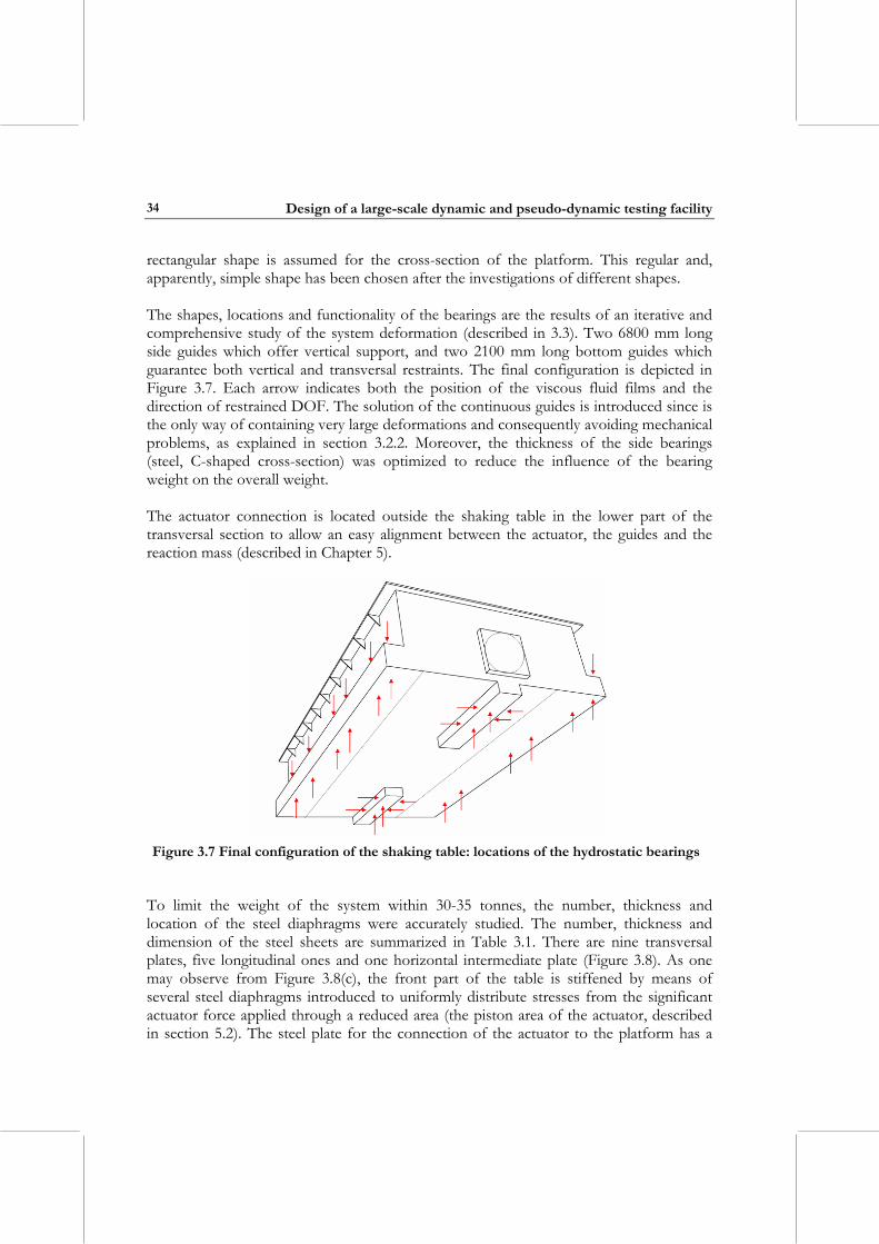
Design of a large-scale dynamic and pseudo-dynamic testing facility
34
rectangular shape is assumed for the cross-section of the platform. This regular and, apparently, simple shape has been chosen after the investigations of different shapes. The shapes, locations and functionality of the bearings are the results of an iterative and comprehensive study of the system deformation (described in 3.3). Two 6800 mm long side guides which offer vertical support, and two 2100 mm long bottom guides which guarantee both vertical and transversal restraints. The final configuration is depicted in Figure 3.7. Each arrow indicates both the position of the viscous fluid films and the direction of restrained DOF. The solution of the continuous guides is introduced since is the only way of containing very large deformations and consequently avoiding mechanical problems, as explained in section 3.2.2. Moreover, the thickness of the side bearings (steel, C-shaped cross-section) was optimized to reduce the influence of the bearing weight on the overall weight. The actuator connection is located outside the shaking table in the lower part of the transversal section to allow an easy alignment between the actuator, the guides and the reaction mass (described in Chapter 5).
Figure 3.7 Final configuration of the shaking table: locations of the hydrostatic bearings
To limit the weight of the system within 30-35 tonnes, the number, thickness and location of the steel diaphragms were accurately studied. The number, thickness and dimension of the steel sheets are summarized in Table 3.1. There are nine transversal plates, five longitudinal ones and one horizontal intermediate plate (Figure 3.8). As one may observe from Figure 3.8(c), the front part of the table is stiffened by means of several steel diaphragms introduced to uniformly distribute stresses from the significant actuator force applied through a reduced area (the piston area of the actuator, described in section 5.2). The steel plate for the connection of the actuator to the platform has a
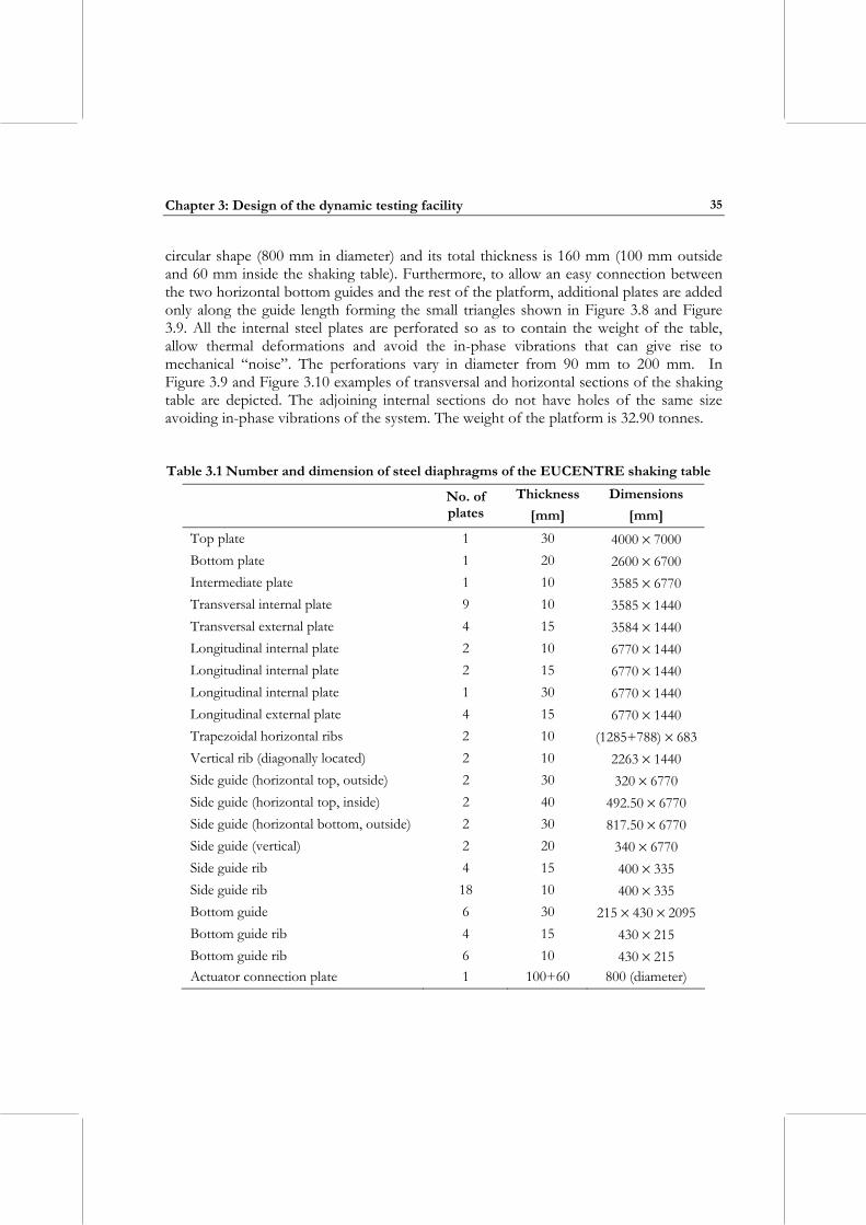
Chapter 3: Design of the dynamic testing facility
35
circular shape (800 mm in diameter) and its total thickness is 160 mm (100 mm outside and 60 mm inside the shaking table). Furthermore, to allow an easy connection between the two horizontal bottom guides and the rest of the platform, additional plates are added only along the guide length forming the small triangles shown in Figure 3.8 and Figure 3.9. All the internal steel plates are perforated so as to contain the weight of the table, allow thermal deformations and avoid the in-phase vibrations that can give rise to mechanical “noise”. The perforations vary in diameter from 90 mm to 200 mm. In Figure 3.9 and Figure 3.10 examples of transversal and horizontal sections of the shaking table are depicted. The adjoining internal sections do not have holes of the same size avoiding in-phase vibrations of the system. The weight of the platform is 32.90 tonnes. Table 3.1 Number and dimension of steel diaphragms of the EUCENTRE shaking table
No. of plates
Thickness [mm]
Dimensions [mm]
Top plate 1 30 4000 × 7000 Bottom plate 1 20 2600 × 6700 Intermediate plate 1 10 3585 × 6770 Transversal internal plate 9 10 3585 × 1440 Transversal external plate 4 15 3584 × 1440 Longitudinal internal plate 2 10 6770 × 1440 Longitudinal internal plate 2 15 6770 × 1440 Longitudinal internal plate 1 30 6770 × 1440 Longitudinal external plate 4 15 6770 × 1440 Trapezoidal horizontal ribs 2 10 (1285+788) × 683 Vertical rib (diagonally located) 2 10 2263 × 1440 Side guide (horizontal top, outside) 2 30 320 × 6770 Side guide (horizontal top, inside) 2 40 492.50 × 6770 Side guide (horizontal bottom, outside) 2 30 817.50 × 6770 Side guide (vertical) 2 20 340 × 6770 Side guide rib 4 15 400 × 335 Side guide rib 18 10 400 × 335 Bottom guide 6 30 215 × 430 × 2095 Bottom guide rib 4 15 430 × 215 Bottom guide rib 6 10 430 × 215 Actuator connection plate 1 100+60 800 (diameter)
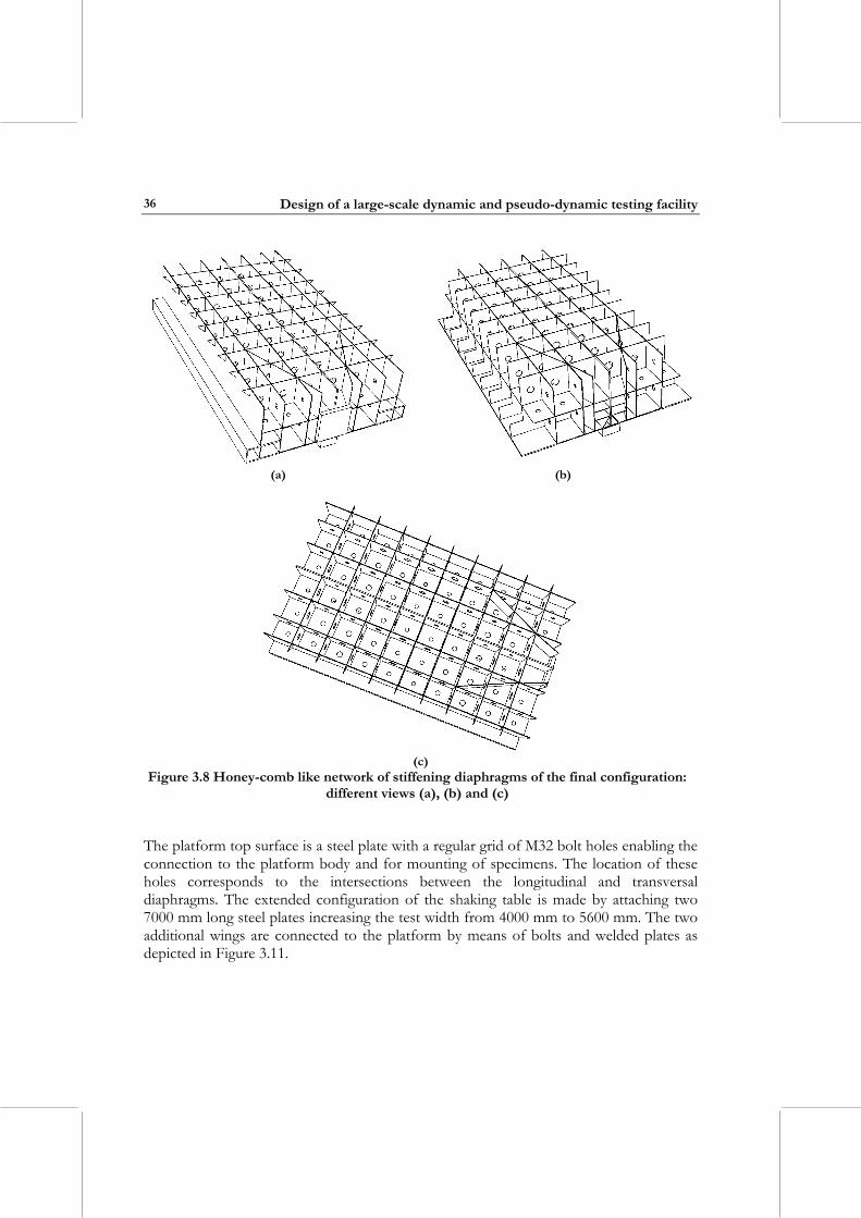
Design of a large-scale dynamic and pseudo-dynamic testing facility
36
(a) (b)
(c)
Figure 3.8 Honey-comb like network of stiffening diaphragms of the final configuration: different views (a), (b) and (c)
The platform top surface is a steel plate with a regular grid of M32 bolt holes enabling the connection to the platform body and for mounting of specimens. The location of these holes corresponds to the intersections between the longitudinal and transversal diaphragms. The extended configuration of the shaking table is made by attaching two 7000 mm long steel plates increasing the test width from 4000 mm to 5600 mm. The two additional wings are connected to the platform by means of bolts and welded plates as depicted in Figure 3.11.
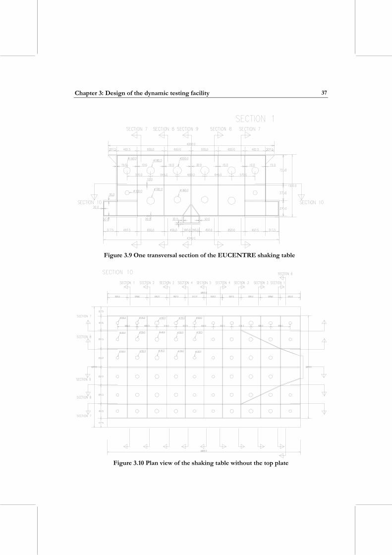
Chapter 3: Design of the dynamic testing facility
37
Figure 3.9 One transversal section of the EUCENTRE shaking table
Figure 3.10 Plan view of the shaking table without the top plate
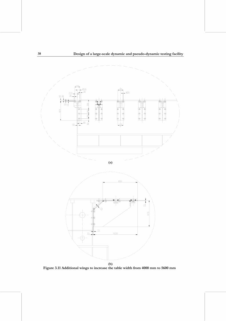
Design of a large-scale dynamic and pseudo-dynamic testing facility
38
(a)
(b)
Figure 3.11 Additional wings to increase the table width from 4000 mm to 5600 mm
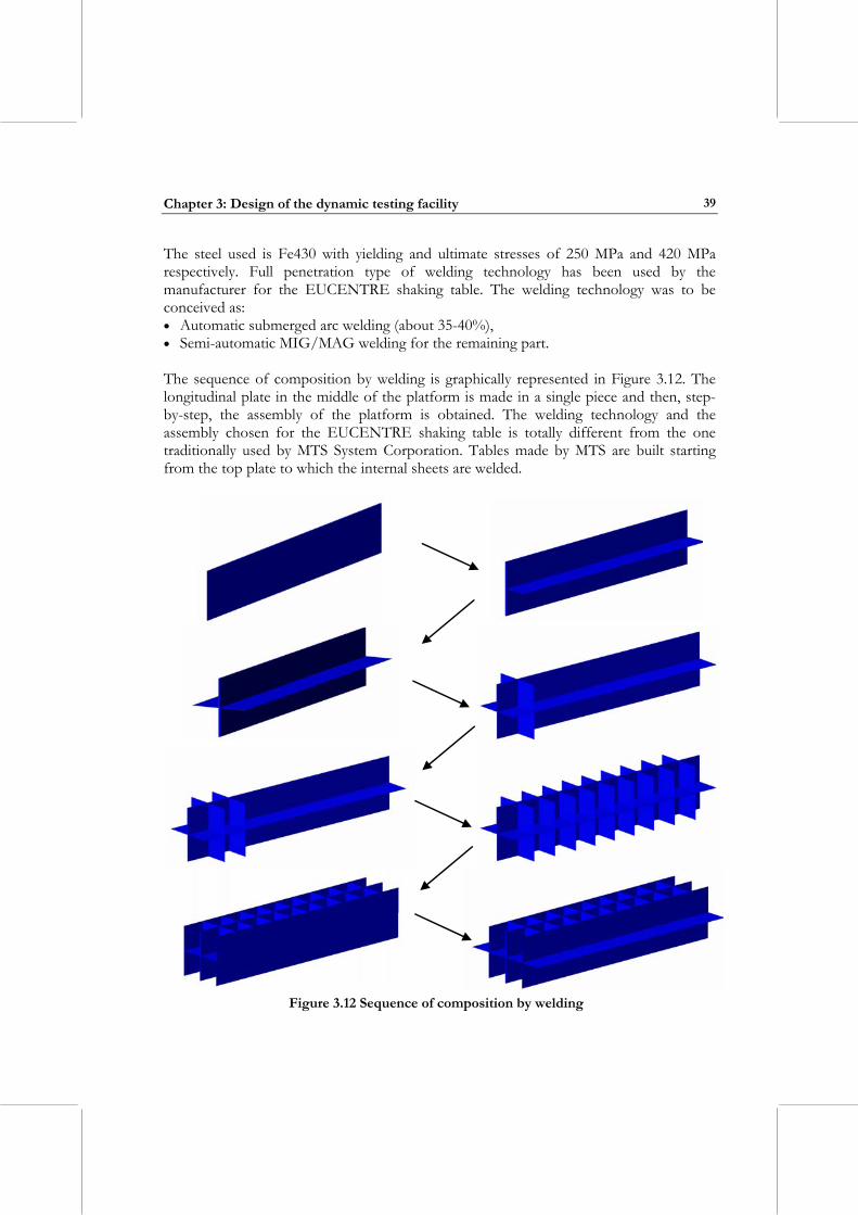
Chapter 3: Design of the dynamic testing facility
39
The steel used is Fe430 with yielding and ultimate stresses of 250 MPa and 420 MPa respectively. Full penetration type of welding technology has been used by the manufacturer for the EUCENTRE shaking table. The welding technology was to be conceived as: • Automatic submerged arc welding (about 35-40%), • Semi-automatic MIG/MAG welding for the remaining part. The sequence of composition by welding is graphically represented in Figure 3.12. The longitudinal plate in the middle of the platform is made in a single piece and then, step-by-step, the assembly of the platform is obtained. The welding technology and the assembly chosen for the EUCENTRE shaking table is totally different from the one traditionally used by MTS System Corporation. Tables made by MTS are built starting from the top plate to which the internal sheets are welded.
Figure 3.12 Sequence of composition by welding
Design of a large-scale dynamic and pseudo-dynamic testing facility
40
A point to be noted is that, due to temperature variations, steel thickness variations and consequently deformations could occur. An accurate evaluation of the stresses caused by temperature variations is required. Some views of the welding technology proposed by the manufacturer [Tecno-cut, 2004] as well as six different types of welded sheets are presented in APPENDIX A. As one may see in APPENDIX A, welding type “1” refers to the top horizontal plate of the shaking table. This plate is not made of a single piece; it is composed of two 7000 mm long sheets welded together in the longitudinal direction.
3.2.2 Design revision history Initially the platform was in the form of an inverted trapezoid with a depth of over 1.5 m at the centre, along with the honeycomb of diaphragms. This solution was adopted to have a very high bending stiffness but it was discarded for the complexity of creating stable and easily controllable hydrostatic bearings. To simplify the bearing design, a rectangular cross-section substituted the trapezoidal one. Using a rectangular shape, the area of the internal diaphragms increases so does the table weight. If the platform weight increases, the maximum feasible payload on the table decreases. So in order to lighten the table an inverted trapezoid shape was further retained in the middle of the platform (in longitudinal direction, as depicted in Figure 2.9). This was possible for the solution proposed for the hydrostatic bearings. Two guides were located beneath the platform and they constrained the transversal motion and the roll rotation. The mechanical constraints to the vertical DOF, the pitch and yaw rotations could be given by means of four lateral hydrostatic bearings (two for each table side), located at the bottom of the platform (as depicted in Figure 2.9). The main problem related to that solution was the abrupt change in stiffness in the longitudinal direction. This caused unacceptable deformations of the platform and bearings with mechanical problems for the system restraining the table motion (as discussed in section 3.2.2). During the sequence of the facility design [Ceresa, 2004], the actuator position was modified several times. Initially the actuator was located inside the platform. That solution could be justified by the aim of limiting occupied space and protecting the actuator from possible damage during experimental tests. Nevertheless, the final choice avoided the disadvantage of a shaking table weakened by the opening for the actuator location. Several changes have been made also for the position of the actuator connection with respect to the centre of gravity of the shaking table. To overcome the above mentioned problems, a much regular shape of the platform was maintained along the overall longitudinal direction and the position of the actuator connection was established to easily allow its alignment with the lateral guides.
Chapter 3: Design of the dynamic testing facility
41
3.3 DESIGN OF THE SYSTEM RESTRAINING THE MOTION OF THE PLATFORM
3.3.1 Final configuration The adopted solution for the system restraining the motion of the platform is represented in Figure 3.7. Its regular shape is optimized in order to minimize deformations of both platform and side bearings and to to avoid concentration of forces. Such a configuration can be adopted considering the hydrostatic solution represented in Figure 3.13 − 6800 mm long bearings for each side of the platform giving the vertical supports and 2 bearings below the table which avoid transversal and vertical movements. The need for adding vertical bearings is due to the overall deformation of the table in its middle part. Hence, additional viscous fluid films are located on the side guides − two 400 mm hydrostatic bearings on both left and right side guides, two 400 mm hydrostatic bearings for both front and back bottom guides. A schematic representation of the hydrostatic bearing location and its functioning is depicted in Figure 3.7. With reference to Figure 3.13, the number and dimensions of the oil surfaces are summarized in Table 3.2. The total number of oil surfaces is computed in the fifth column of the table. For the side guides, 2×3×2 implies 2 adjacent 400 mm long viscous fluid films to form one hydrostatic bearing, times 3 since the bearings are three for each side, times 2 considering both left and right side guides. For the bottom guides, 2×2 implies 2 adjacent 400 mm long oil films, times 2 considering the front and back guides.
Table 3.2 Hydrostatic bearings: number, location and area
Location Restraint Area [mm2]
Aeff [mm2]
Total no. thin viscous fluid films
Side guides vertical top 400 × 320 360 × 280 2×3×2 = 12 bottom 400 × 480 360 × 440 2×3×2 = 12
Bottom guides vertical 400 × 430 360 × 390 2×2 = 4 Bottom guides transversal 400 × 200 360 × 160 2×2 = 4
Eq. (3.1) is used to compute hydrostatic stiffness of the thin viscous fluid films. In Table 3.3 and Table 3.4, the stiffnesses are computed for two different oil thicknesses - 0.05 mm and 0.07 mm. The decision to assume the viscous fluid thickness up to 0.05–0.07 mm was taken in consultation with the manufacturer. In the analyses performed, the 0.05 mm thick viscous fluid was considered since it ensures stiffer restraint (section 3.6). Considering the dynamic viscosity of the oil equal to 0.07 Ns/m2, the thickness of the oil film h of 0.05 mm, and the metallic area of the bearings, Amet given by the sum of the area in Table 3.2, the trend of the bearing friction force vs. the table velocity is determined and shown in Figure 3.14.
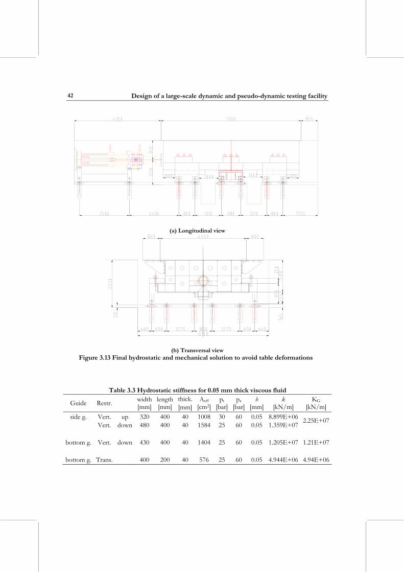
Design of a large-scale dynamic and pseudo-dynamic testing facility
42
(a) Longitudinal view
(b) Transversal view Figure 3.13 Final hydrostatic and mechanical solution to avoid table deformations
Table 3.3 Hydrostatic stiffness for 0.05 mm thick viscous fluid
Guide Restr. width [mm]
length[mm]
thick.[mm]
Aeff [cm2]
pt [bar]
pa [bar]
h [mm]
k [kN/m]
KG [kN/m]
side g. Vert. up 320 400 40 1008 30 60 0.05 8.899E+06 Vert. down 480 400 40 1584 25 60 0.05 1.359E+07
2.25E+07
bottom g. Vert. down 430 400 40 1404 25 60 0.05 1.205E+07 1.21E+07
bottom g. Trans. 400 200 40 576 25 60 0.05 4.944E+06 4.94E+06
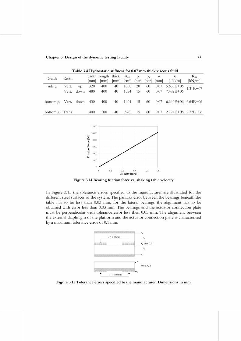
Chapter 3: Design of the dynamic testing facility
43
Table 3.4 Hydrostatic stiffness for 0.07 mm thick viscous fluid
Guide Restr. width [mm]
length[mm]
thick.[mm]
Aeff [cm2]
pt [bar]
pa [bar]
h [mm]
k [kN/m]
KG [kN/m]
side g. Vert. up 320 400 40 1008 20 60 0.07 5.650E+06 Vert. down 480 400 40 1584 15 60 0.07 7.492E+06
1.31E+07
bottom g. Vert. down 430 400 40 1404 15 60 0.07 6.640E+06 6.64E+06
bottom g. Trans. 400 200 40 576 15 60 0.07 2.724E+06 2.72E+06
0
2000
4000
6000
8000
10000
12000
0 0.3 0.6 0.9 1.2 1.5Velocity [m/s]
Fric
tion
Forc
e [N
]
Figure 3.14 Bearing friction force vs. shaking table velocity In Figure 3.15 the tolerance errors specified to the manufacturer are illustrated for the different steel surfaces of the system. The parallax error between the bearings beneath the table has to be less than 0.03 mm; for the lateral bearings the alignment has to be obtained with error less than 0.03 mm. The bearings and the actuator connection plate must be perpendicular with tolerance error less then 0.05 mm. The alignment between the external diaphragm of the platform and the actuator connection plate is characterised by a maximum tolerance error of 0.1 mm.
// 0.03mm
max 0.1
//
//
A
B
0.05 A, B
0.03mm
Figure 3.15 Tolerance errors specified to the manufacturer. Dimensions in mm
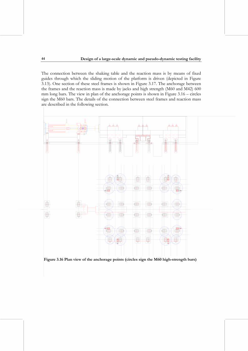
Design of a large-scale dynamic and pseudo-dynamic testing facility
44
The connection between the shaking table and the reaction mass is by means of fixed guides through which the sliding motion of the platform is driven (depicted in Figure 3.13). One section of these steel frames is shown in Figure 3.17. The anchorage between the frames and the reaction mass is made by jacks and high strength (M60 and M42) 600 mm long bars. The view in plan of the anchorage points is shown in Figure 3.16 – circles sign the M60 bars. The details of the connection between steel frames and reaction mass are described in the following section.
Figure 3.16 Plan view of the anchorage points (circles sign the M60 high-strength bars)
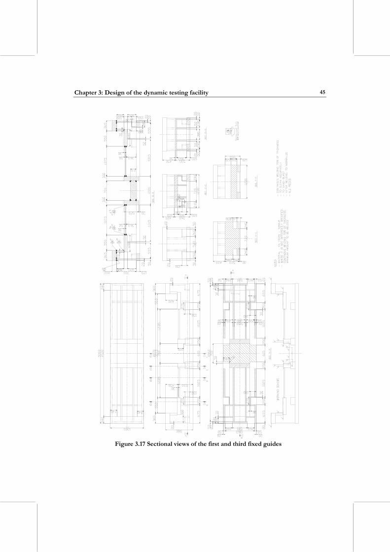
Chapter 3: Design of the dynamic testing facility
45
Figure 3.17 Sectional views of the first and third fixed guides
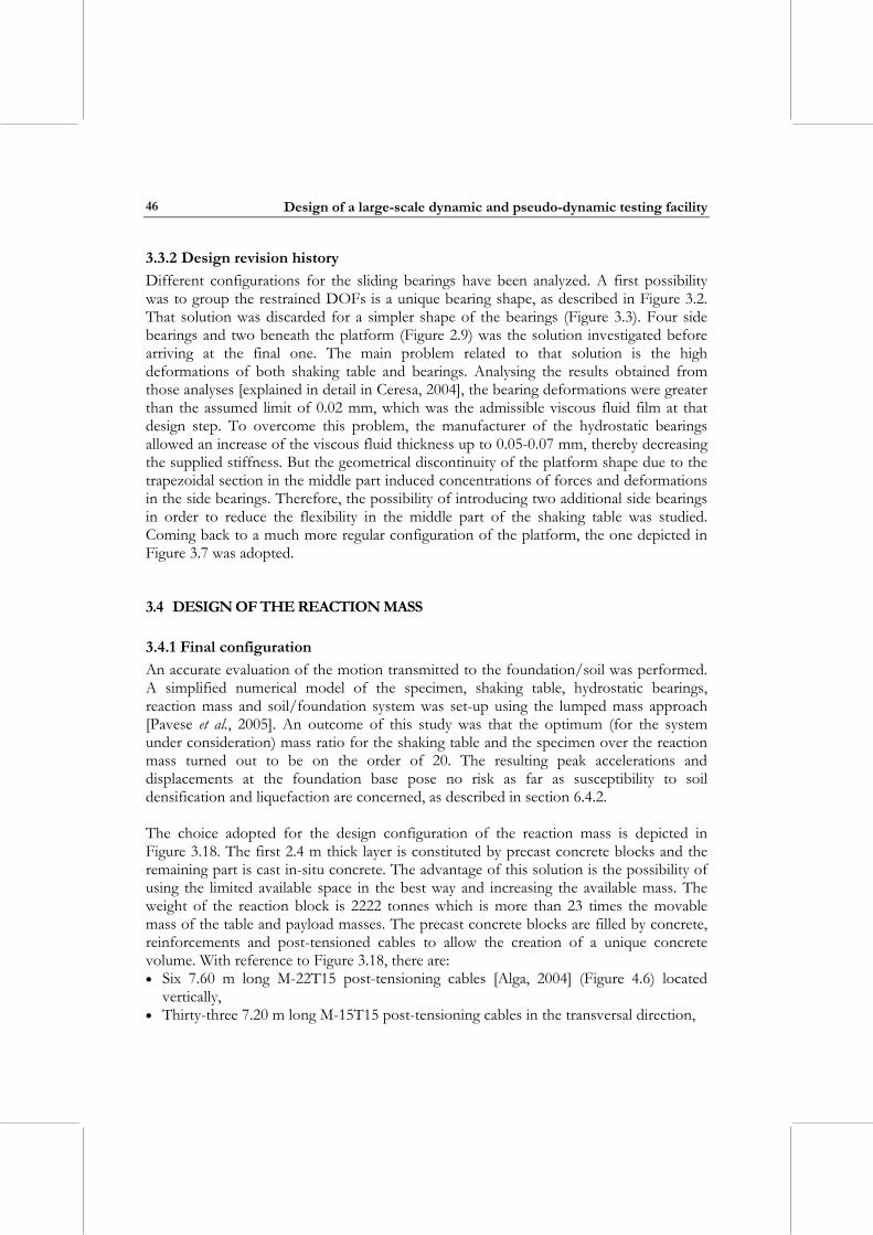
Design of a large-scale dynamic and pseudo-dynamic testing facility
46
3.3.2 Design revision history Different configurations for the sliding bearings have been analyzed. A first possibility was to group the restrained DOFs is a unique bearing shape, as described in Figure 3.2. That solution was discarded for a simpler shape of the bearings (Figure 3.3). Four side bearings and two beneath the platform (Figure 2.9) was the solution investigated before arriving at the final one. The main problem related to that solution is the high deformations of both shaking table and bearings. Analysing the results obtained from those analyses [explained in detail in Ceresa, 2004], the bearing deformations were greater than the assumed limit of 0.02 mm, which was the admissible viscous fluid film at that design step. To overcome this problem, the manufacturer of the hydrostatic bearings allowed an increase of the viscous fluid thickness up to 0.05-0.07 mm, thereby decreasing the supplied stiffness. But the geometrical discontinuity of the platform shape due to the trapezoidal section in the middle part induced concentrations of forces and deformations in the side bearings. Therefore, the possibility of introducing two additional side bearings in order to reduce the flexibility in the middle part of the shaking table was studied. Coming back to a much more regular configuration of the platform, the one depicted in Figure 3.7 was adopted.
3.4 DESIGN OF THE REACTION MASS
3.4.1 Final configuration An accurate evaluation of the motion transmitted to the foundation/soil was performed. A simplified numerical model of the specimen, shaking table, hydrostatic bearings, reaction mass and soil/foundation system was set-up using the lumped mass approach [Pavese et al., 2005]. An outcome of this study was that the optimum (for the system under consideration) mass ratio for the shaking table and the specimen over the reaction mass turned out to be on the order of 20. The resulting peak accelerations and displacements at the foundation base pose no risk as far as susceptibility to soil densification and liquefaction are concerned, as described in section 6.4.2. The choice adopted for the design configuration of the reaction mass is depicted in Figure 3.18. The first 2.4 m thick layer is constituted by precast concrete blocks and the remaining part is cast in-situ concrete. The advantage of this solution is the possibility of using the limited available space in the best way and increasing the available mass. The weight of the reaction block is 2222 tonnes which is more than 23 times the movable mass of the table and payload masses. The precast concrete blocks are filled by concrete, reinforcements and post-tensioned cables to allow the creation of a unique concrete volume. With reference to Figure 3.18, there are: • Six 7.60 m long M-22T15 post-tensioning cables [Alga, 2004] (Figure 4.6) located
vertically, • Thirty-three 7.20 m long M-15T15 post-tensioning cables in the transversal direction,
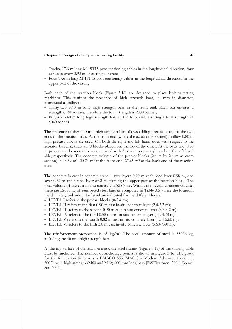
Chapter 3: Design of the dynamic testing facility
47
• Twelve 17.6 m long M-15T15 post-tensioning cables in the longitudinal direction, four cables in every 0.90 m of casting concrete,
• Four 17.6 m long M-15T15 post-tensioning cables in the longitudinal direction, in the upper part of the casting.
Both ends of the reaction block (Figure 3.18) are designed to place isolator-testing machines. This justifies the presence of high strength bars, 40 mm in diameter, distributed as follows: • Thirty-two 3.40 m long high strength bars in the front end. Each bar ensures a
strength of 90 tonnes, therefore the total strength is 2880 tonnes, • Fifty-six 3.40 m long high strength bars in the back end, assuring a total strength of
5040 tonnes. The presence of these 40 mm high strength bars allows adding precast blocks at the two ends of the reaction mass. At the front end (where the actuator is located), hollow 0.80 m high precast blocks are used. On both the right and left hand sides with respect to the actuator location, there are 3 blocks placed one on top of the other. At the back end, 0.80 m precast solid concrete blocks are used with 3 blocks on the right and on the left hand side, respectively. The concrete volume of the precast blocks (2.4 m by 2.4 m as cross section) is 48.39 m3: 20.74 m3 at the front end, 27.65 m3 at the back end of the reaction mass. The concrete is cast in separate steps − two layers 0.90 m each, one layer 0.58 m, one layer 0.82 m and a final layer of 2 m forming the upper part of the reaction block. The total volume of the cast in-situ concrete is 838.7 m3. Within the overall concrete volume, there are 52055 kg of reinforced steel bars as computed in Table 3.5 where the location, the diameter, and amount of steel are indicated for the different levels: • LEVEL I refers to the precast blocks (0-2.4 m); • LEVEL II refers to the first 0.90 m cast in-situ concrete layer (2.4-3.3 m); • LEVEL III refers to the second 0.90 m cast in-situ concrete layer (3.3-4.2 m); • LEVEL IV refers to the third 0.58 m cast in-situ concrete layer (4.2-4.78 m); • LEVEL V refers to the fourth 0.82 m cast in-situ concrete layer (4.78-5.60 m); • LEVEL VI refers to the fifth 2.0 m cast in-situ concrete layer (5.60-7.60 m). The reinforcement proportion is 63 kg/m3. The total amount of steel is 55006 kg, including the 40 mm high strength bars. At the top surface of the reaction mass, the steel frames (Figure 3.17) of the shaking table must be anchored. The number of anchorage points is shown in Figure 3.16. The grout for the foundation tie beams is EMACO S55 [MAC Spa Modern Advanced Concrete, 2002], with high strength (M60 and M42) 600 mm long bars [BWFixatoren, 2004; Tecno-cut, 2004].
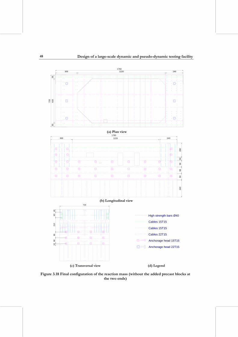
Design of a large-scale dynamic and pseudo-dynamic testing facility
48
1220
610
1760
720
5555
300 240
(a) Plan view
1760
240
9090
9050
200
300 1220 240
(b) Longitudinal view
4080
210
8686
18
720
High strength bars Ø40
Cables 15T15
Cables 22T15
Anchorage head 15T15
Anchorage head 22T15
Cables 15T15
(c) Transversal view (d) Legend
Figure 3.18 Final configuration of the reaction mass (without the added precast blocks at the two ends)
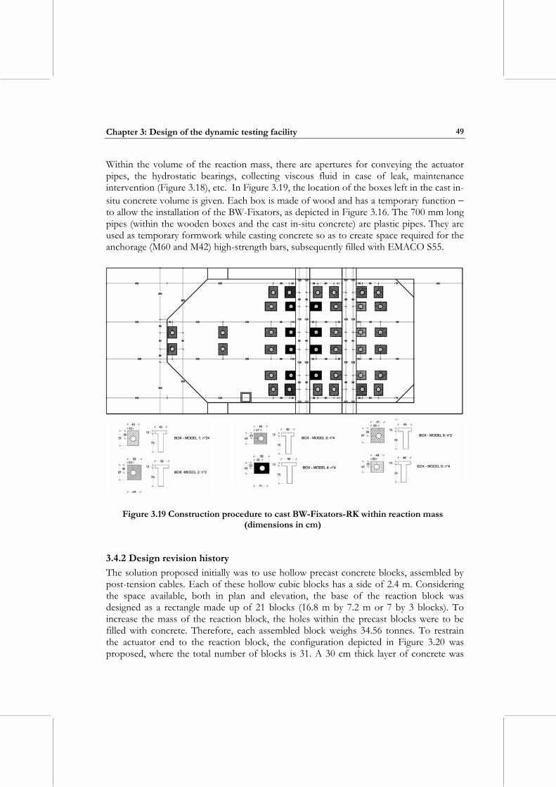
Chapter 3: Design of the dynamic testing facility
49
Within the volume of the reaction mass, there are apertures for conveying the actuator pipes, the hydrostatic bearings, collecting viscous fluid in case of leak, maintenance intervention (Figure 3.18), etc. In Figure 3.19, the location of the boxes left in the cast in-situ concrete volume is given. Each box is made of wood and has a temporary function − to allow the installation of the BW-Fixators, as depicted in Figure 3.16. The 700 mm long pipes (within the wooden boxes and the cast in-situ concrete) are plastic pipes. They are used as temporary formwork while casting concrete so as to create space required for the anchorage (M60 and M42) high-strength bars, subsequently filled with EMACO S55.
Figure 3.19 Construction procedure to cast BW-Fixators-RK within reaction mass (dimensions in cm)
3.4.2 Design revision history The solution proposed initially was to use hollow precast concrete blocks, assembled by post-tension cables. Each of these hollow cubic blocks has a side of 2.4 m. Considering the space available, both in plan and elevation, the base of the reaction block was designed as a rectangle made up of 21 blocks (16.8 m by 7.2 m or 7 by 3 blocks). To increase the mass of the reaction block, the holes within the precast blocks were to be filled with concrete. Therefore, each assembled block weighs 34.56 tonnes. To restrain the actuator end to the reaction block, the configuration depicted in Figure 3.20 was proposed, where the total number of blocks is 31. A 30 cm thick layer of concrete was
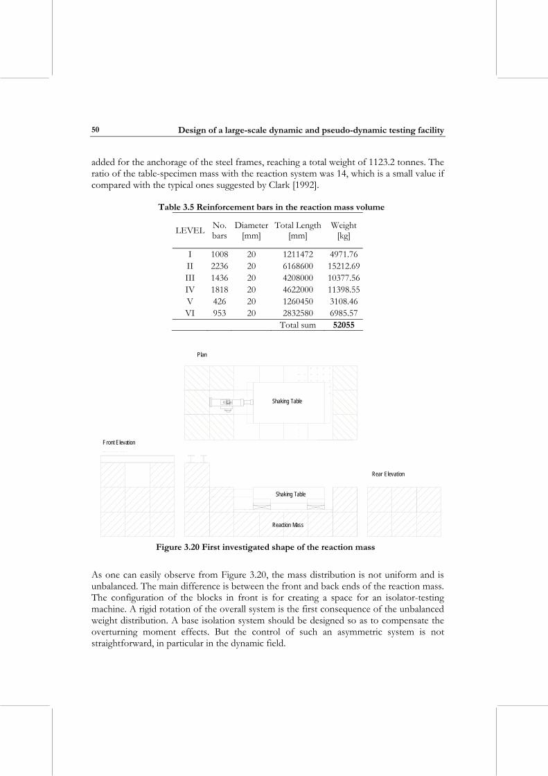
Design of a large-scale dynamic and pseudo-dynamic testing facility
50
added for the anchorage of the steel frames, reaching a total weight of 1123.2 tonnes. The ratio of the table-specimen mass with the reaction system was 14, which is a small value if compared with the typical ones suggested by Clark [1992].
Table 3.5 Reinforcement bars in the reaction mass volume
LEVEL No. bars
Diameter [mm]
Total Length [mm]
Weight [kg]
I 1008 20 1211472 4971.76II 2236 20 6168600 15212.69III 1436 20 4208000 10377.56IV 1818 20 4622000 11398.55V 426 20 1260450 3108.46VI 953 20 2832580 6985.57
Total sum 52055
Shaking Table
Reaction Mass
Shaking Table
In plan view
In front view
From the back
Front Elevation
Plan
Rear Elevation
Figure 3.20 First investigated shape of the reaction mass
As one can easily observe from Figure 3.20, the mass distribution is not uniform and is unbalanced. The main difference is between the front and back ends of the reaction mass. The configuration of the blocks in front is for creating a space for an isolator-testing machine. A rigid rotation of the overall system is the first consequence of the unbalanced weight distribution. A base isolation system should be designed so as to compensate the overturning moment effects. But the control of such an asymmetric system is not straightforward, in particular in the dynamic field.
Chapter 3: Design of the dynamic testing facility
51
Changes to the initially investigated configuration were required when the actual dimensions of the actuator were defined by the MTS System Corporation [2004]. The available space was to be subdivided between the size of the table, its stroke, the actuator length, the actuator connection plates with the reaction mass and the platform itself. A modification of the assembled reaction mass was considered. The end blocks at the back were changed reducing their width to 1.2 m instead of 2.4 m. The new width was determined by the economic choice of using the same formwork for the all precast blocks. If this solution solved space and cost limitations, it contributed to unbalancing the mass distribution, and further, to reduce the reaction mass. To balance the distribution of the weights and to increase the mass ratio between the table-specimen and the reaction system, a new configuration of the reaction mass was introduced. And this design choice was related to the changed configuration of the platform itself. The reaction block, depicted in Figure 6.19 (on left), was constituted by 31 precast concrete blocks, 0.40 m thick reinforced concrete (RC) layer beneath the fixed guides (size 12 m long by 7.2 m width), and two boundary 2.0 m high RC walls of thickness 0.60 m and length 12 m. The thickness of the two boundary walls was justified by the possibility of adding two lateral steel wings to the platform to increase its area in plan. The total mass of the reaction system was increased up to 1229.76 tonnes which is 15.4 times the table-specimen mass. From the numerical simulations of the dynamic soil-structure interaction (section 6.4.1), the configuration in the right hand side of Figure 6.19 was studied before arriving at the final solution described in section 3.4.1. For further information, the reader is referred to Ceresa [2004] where a thorough explanation of the studied cases is given.
3.5 DESIGN OF THE ISOLATION SYSTEM
3.5.1 Final solution The final choice for the dynamic facility of the EUCENTRE was to increase the mass of the reaction block (Section 3.4) without the isolation and damping systems. The decision was taken according the results of an accurate study [Pavese et al., 2005] of the motion transmitted to the underlying soil (described in Section 6.4). The designers decided on the basis of the comparison of two configurations - the reaction mass and the isolation system of Figure 6.19 (on the left) and the reaction mass rigidly connected to the foundation without isolation (Figure 6.19, on the right). The first was discarded since the amplification of transmitted motion is unacceptable at the resonance frequency of the system. By increasing the reaction mass, its ratio to the movable mass (given by both the specimen and table masses) increases allowing a reduction of accelerations and displacements transmitted to the soil. From results of the dynamic soil-structure
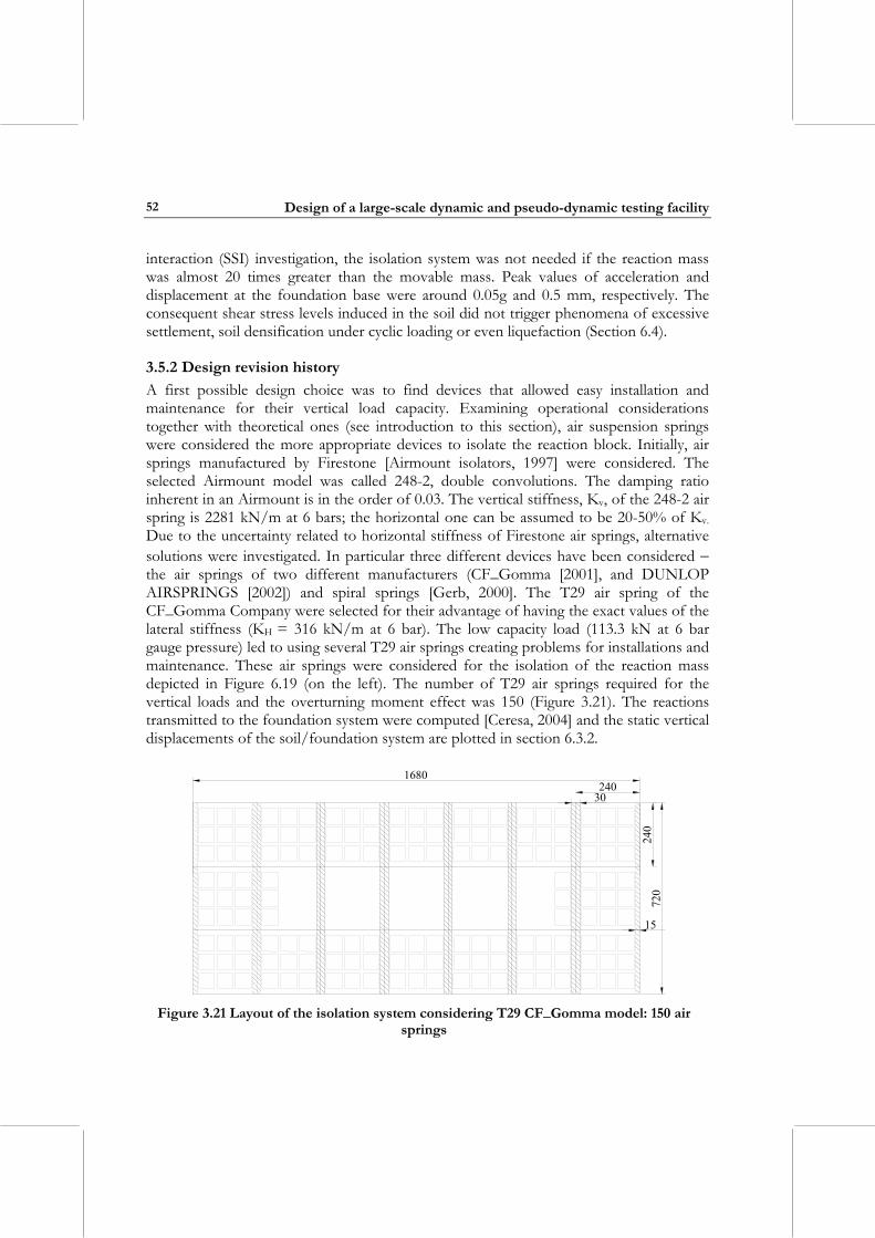
Design of a large-scale dynamic and pseudo-dynamic testing facility
52
interaction (SSI) investigation, the isolation system was not needed if the reaction mass was almost 20 times greater than the movable mass. Peak values of acceleration and displacement at the foundation base were around 0.05g and 0.5 mm, respectively. The consequent shear stress levels induced in the soil did not trigger phenomena of excessive settlement, soil densification under cyclic loading or even liquefaction (Section 6.4).
3.5.2 Design revision history A first possible design choice was to find devices that allowed easy installation and maintenance for their vertical load capacity. Examining operational considerations together with theoretical ones (see introduction to this section), air suspension springs were considered the more appropriate devices to isolate the reaction block. Initially, air springs manufactured by Firestone [Airmount isolators, 1997] were considered. The selected Airmount model was called 248-2, double convolutions. The damping ratio inherent in an Airmount is in the order of 0.03. The vertical stiffness, Kv, of the 248-2 air spring is 2281 kN/m at 6 bars; the horizontal one can be assumed to be 20-50% of Kv.
Due to the uncertainty related to horizontal stiffness of Firestone air springs, alternative solutions were investigated. In particular three different devices have been considered − the air springs of two different manufacturers (CF_Gomma [2001], and DUNLOP AIRSPRINGS [2002]) and spiral springs [Gerb, 2000]. The T29 air spring of the CF_Gomma Company were selected for their advantage of having the exact values of the lateral stiffness (KH = 316 kN/m at 6 bar). The low capacity load (113.3 kN at 6 bar gauge pressure) led to using several T29 air springs creating problems for installations and maintenance. These air springs were considered for the isolation of the reaction mass depicted in Figure 6.19 (on the left). The number of T29 air springs required for the vertical loads and the overturning moment effect was 150 (Figure 3.21). The reactions transmitted to the foundation system were computed [Ceresa, 2004] and the static vertical displacements of the soil/foundation system are plotted in section 6.3.2.
240
240
30
720
1680
15
Figure 3.21 Layout of the isolation system considering T29 CF_Gomma model: 150 air
springs
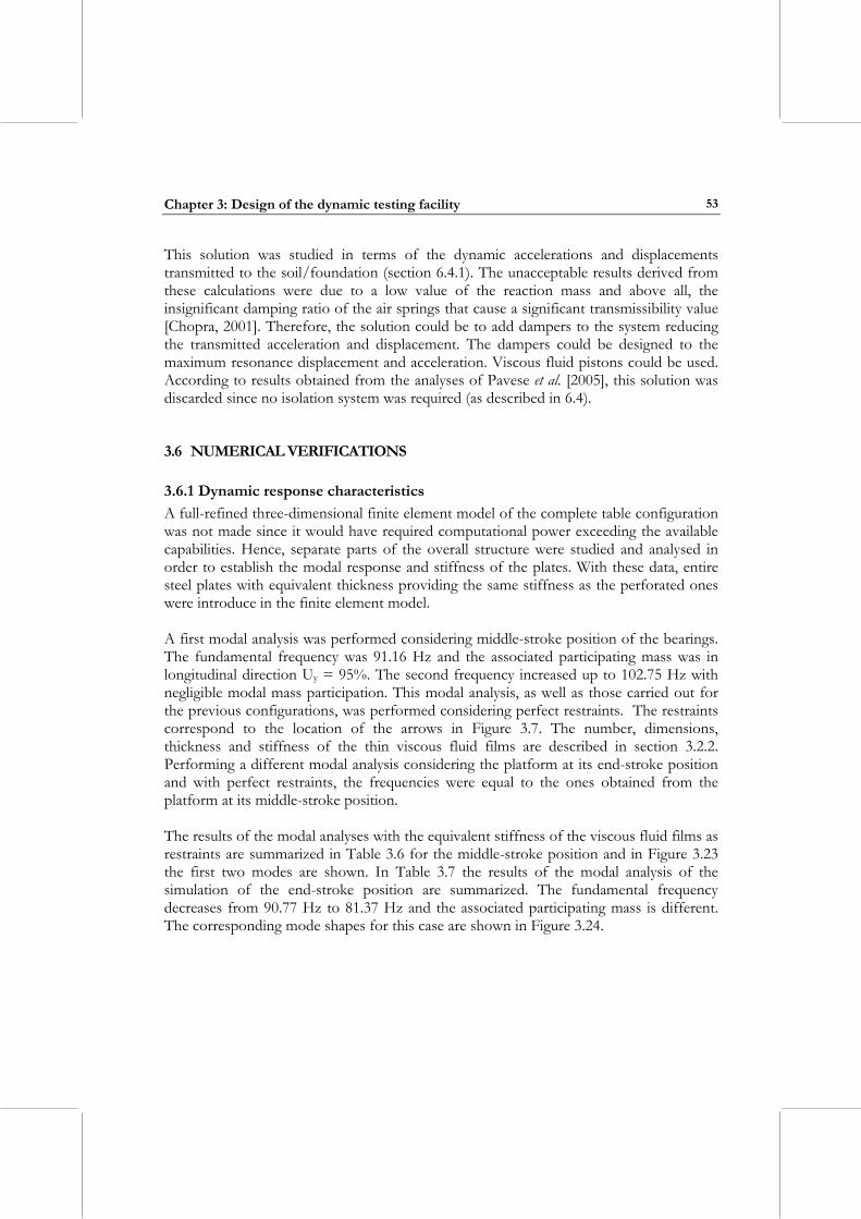
Chapter 3: Design of the dynamic testing facility
53
This solution was studied in terms of the dynamic accelerations and displacements transmitted to the soil/foundation (section 6.4.1). The unacceptable results derived from these calculations were due to a low value of the reaction mass and above all, the insignificant damping ratio of the air springs that cause a significant transmissibility value [Chopra, 2001]. Therefore, the solution could be to add dampers to the system reducing the transmitted acceleration and displacement. The dampers could be designed to the maximum resonance displacement and acceleration. Viscous fluid pistons could be used. According to results obtained from the analyses of Pavese et al. [2005], this solution was discarded since no isolation system was required (as described in 6.4).
3.6 NUMERICAL VERIFICATIONS
3.6.1 Dynamic response characteristics A full-refined three-dimensional finite element model of the complete table configuration was not made since it would have required computational power exceeding the available capabilities. Hence, separate parts of the overall structure were studied and analysed in order to establish the modal response and stiffness of the plates. With these data, entire steel plates with equivalent thickness providing the same stiffness as the perforated ones were introduce in the finite element model. A first modal analysis was performed considering middle-stroke position of the bearings. The fundamental frequency was 91.16 Hz and the associated participating mass was in longitudinal direction Uy = 95%. The second frequency increased up to 102.75 Hz with negligible modal mass participation. This modal analysis, as well as those carried out for the previous configurations, was performed considering perfect restraints. The restraints correspond to the location of the arrows in Figure 3.7. The number, dimensions, thickness and stiffness of the thin viscous fluid films are described in section 3.2.2. Performing a different modal analysis considering the platform at its end-stroke position and with perfect restraints, the frequencies were equal to the ones obtained from the platform at its middle-stroke position. The results of the modal analyses with the equivalent stiffness of the viscous fluid films as restraints are summarized in Table 3.6 for the middle-stroke position and in Figure 3.23 the first two modes are shown. In Table 3.7 the results of the modal analysis of the simulation of the end-stroke position are summarized. The fundamental frequency decreases from 90.77 Hz to 81.37 Hz and the associated participating mass is different. The corresponding mode shapes for this case are shown in Figure 3.24.
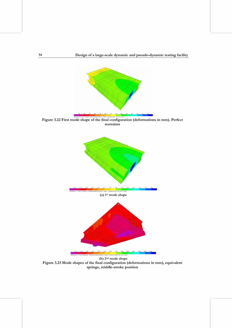
Design of a large-scale dynamic and pseudo-dynamic testing facility
54
Figure 3.22 First mode shape of the final configuration (deformations in mm). Perfect
restraints
(a) 1st mode shape
(b) 2nd mode shape
Figure 3.23 Mode shapes of the final configuration (deformations in mm), equivalent springs, middle-stroke position
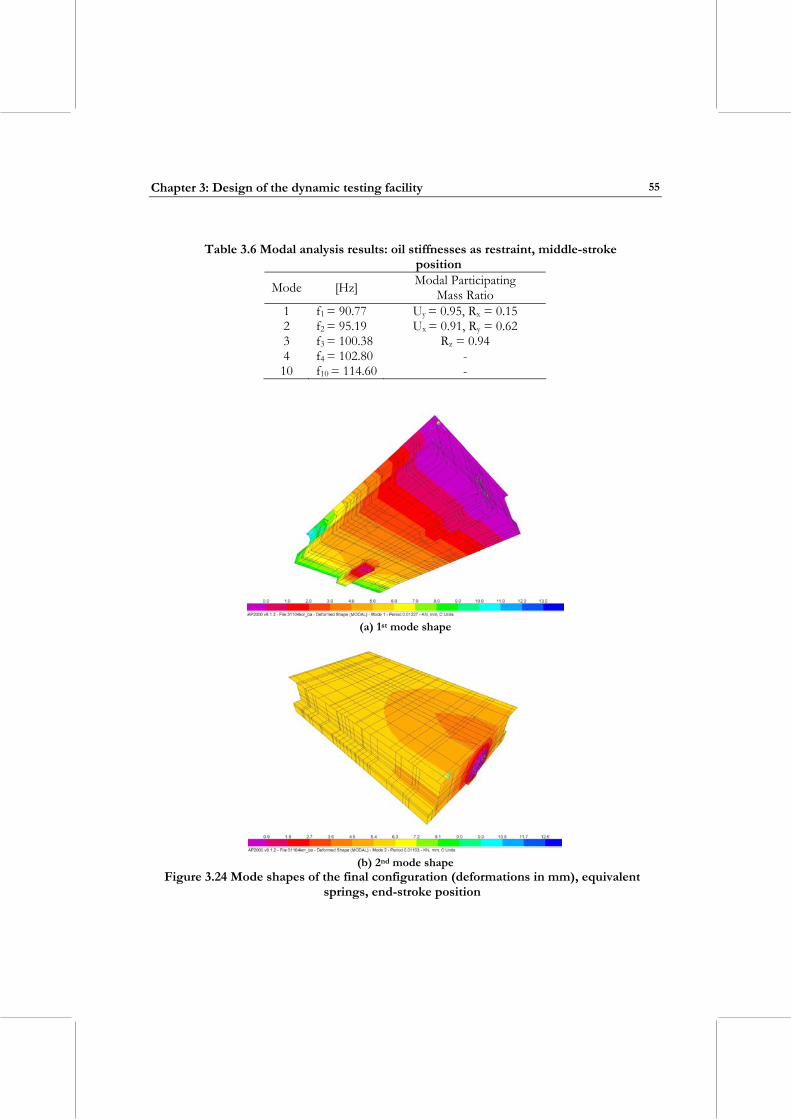
Chapter 3: Design of the dynamic testing facility
55
Table 3.6 Modal analysis results: oil stiffnesses as restraint, middle-stroke
position
Mode [Hz] Modal Participating Mass Ratio
1 f1 = 90.77 Uy = 0.95, Rx = 0.15 2 f2 = 95.19 Ux = 0.91, Ry = 0.62 3 f3 = 100.38 Rz = 0.94 4 f4 = 102.80 - 10 f10 = 114.60 -
(a) 1st mode shape
(b) 2nd mode shape
Figure 3.24 Mode shapes of the final configuration (deformations in mm), equivalent springs, end-stroke position
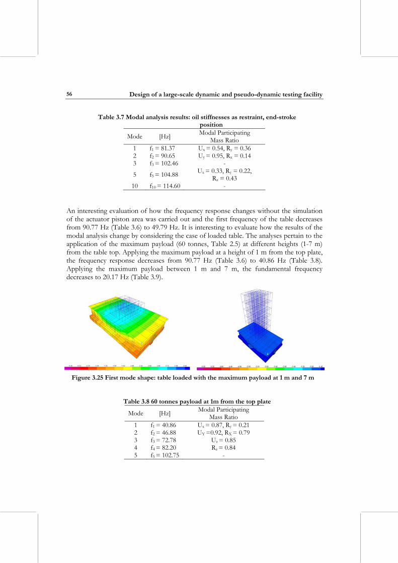
Design of a large-scale dynamic and pseudo-dynamic testing facility
56
Table 3.7 Modal analysis results: oil stiffnesses as restraint, end-stroke position
Mode [Hz] Modal Participating Mass Ratio
1 f1 = 81.37 Ux = 0.54, Ry = 0.36 2 f2 = 90.65 Uy = 0.95, Rx = 0.14 3 f3 = 102.46 -
5 f5 = 104.88 Ux = 0.33, Ry = 0.22, Rz = 0.43
10 f10 = 114.60 - An interesting evaluation of how the frequency response changes without the simulation of the actuator piston area was carried out and the first frequency of the table decreases from 90.77 Hz (Table 3.6) to 49.79 Hz. It is interesting to evaluate how the results of the modal analysis change by considering the case of loaded table. The analyses pertain to the application of the maximum payload (60 tonnes, Table 2.5) at different heights (1-7 m) from the table top. Applying the maximum payload at a height of 1 m from the top plate, the frequency response decreases from 90.77 Hz (Table 3.6) to 40.86 Hz (Table 3.8). Applying the maximum payload between 1 m and 7 m, the fundamental frequency decreases to 20.17 Hz (Table 3.9).
Figure 3.25 First mode shape: table loaded with the maximum payload at 1 m and 7 m
Table 3.8 60 tonnes payload at 1m from the top plate
Mode [Hz] Modal Participating Mass Ratio
1 f1 = 40.86 Ux = 0.87, Ry = 0.21 2 f2 = 46.88 UY =0.92, RX = 0.79 3 f3 = 72.78 Uz = 0.85 4 f4 = 82.20 Rz = 0.84 5 f5 = 102.75 -
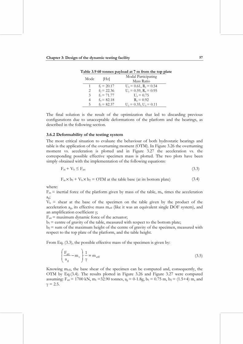
Chapter 3: Design of the dynamic testing facility
57
Table 3.9 60 tonnes payload at 7 m from the top plate
Mode [Hz] Modal Participating Mass Ratio
1 f1 = 20.17 Ux = 0.61, Ry = 0.54 2 f2 = 22.36 Uy = 0.59, Rx = 0.95 3 f3 = 71.77 Uz = 0.75 4 f4 = 82.18 Rz = 0.92 5 f5 = 82.37 Uy = 0.35, Uz = 0.11
The final solution is the result of the optimization that led to discarding previous configurations due to unacceptable deformations of the platform and the bearings, as described in the following section.
3.6.2 Deformability of the testing system The most critical situation to evaluate the behaviour of both hydrostatic bearings and table is the application of the overturning moment (OTM). In Figure 3.26 the overturning moment vs. acceleration is plotted and in Figure 3.27 the acceleration vs. the corresponding possible effective specimen mass is plotted. The two plots have been simply obtained with the implementation of the following equations:
Fin + Vb ≤ Fatt (3.3)
Fin × b1 + Vb × b2 = OTM at the table base (at its bottom plate) (3.4)
where: Fin = inertial force of the platform given by mass of the table, mt, times the acceleration ag; Vb = shear at the base of the specimen on the table given by the product of the acceleration ag, its effective mass meff (like it was an equivalent single DOF system), and an amplification coefficient γ; Fatt = maximum dynamic force of the actuator; b1 = centre of gravity of the table, measured with respect to the bottom plate; b2 = sum of the maximum height of the centre of gravity of the specimen, measured with respect to the top plate of the platform, and the table height. From Eq. (3.3), the possible effective mass of the specimen is given by:
efftg
att mγ1m
aF
=⋅⎟⎟⎠
⎞⎜⎜⎝
⎛− (3.5)
Knowing meff, the base shear of the specimen can be computed and, consequently, the OTM by Eq.(3.4). The results plotted in Figure 3.26 and Figure 3.27 were computed assuming: Fatt = 1700 kN, mt =32.90 tonnes, ag = 0-1.8g, b1 = 0.75 m, b2 = (1.5+4) m, and γ = 2.5.
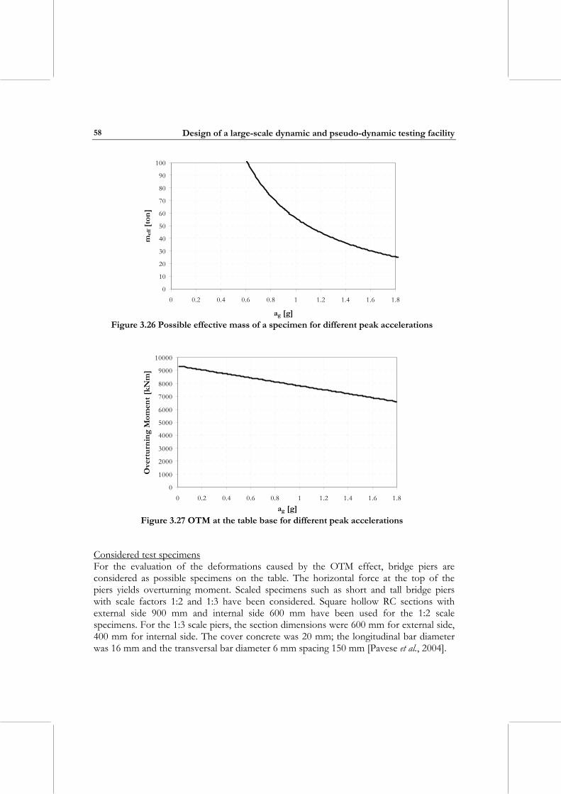
Design of a large-scale dynamic and pseudo-dynamic testing facility
58
0
10
20
30
40
50
60
70
80
90
100
0 0.2 0.4 0.6 0.8 1 1.2 1.4 1.6 1.8
ag [g]
mef
f [to
n]
Figure 3.26 Possible effective mass of a specimen for different peak accelerations
0
1000
2000
3000
4000
5000
6000
7000
8000
9000
10000
0 0.2 0.4 0.6 0.8 1 1.2 1.4 1.6 1.8ag [g]
Ove
rtur
ning
Mom
ent [
kNm
]
Figure 3.27 OTM at the table base for different peak accelerations
Considered test specimens For the evaluation of the deformations caused by the OTM effect, bridge piers are considered as possible specimens on the table. The horizontal force at the top of the piers yields overturning moment. Scaled specimens such as short and tall bridge piers with scale factors 1:2 and 1:3 have been considered. Square hollow RC sections with external side 900 mm and internal side 600 mm have been used for the 1:2 scale specimens. For the 1:3 scale piers, the section dimensions were 600 mm for external side, 400 mm for internal side. The cover concrete was 20 mm; the longitudinal bar diameter was 16 mm and the transversal bar diameter 6 mm spacing 150 mm [Pavese et al., 2004].
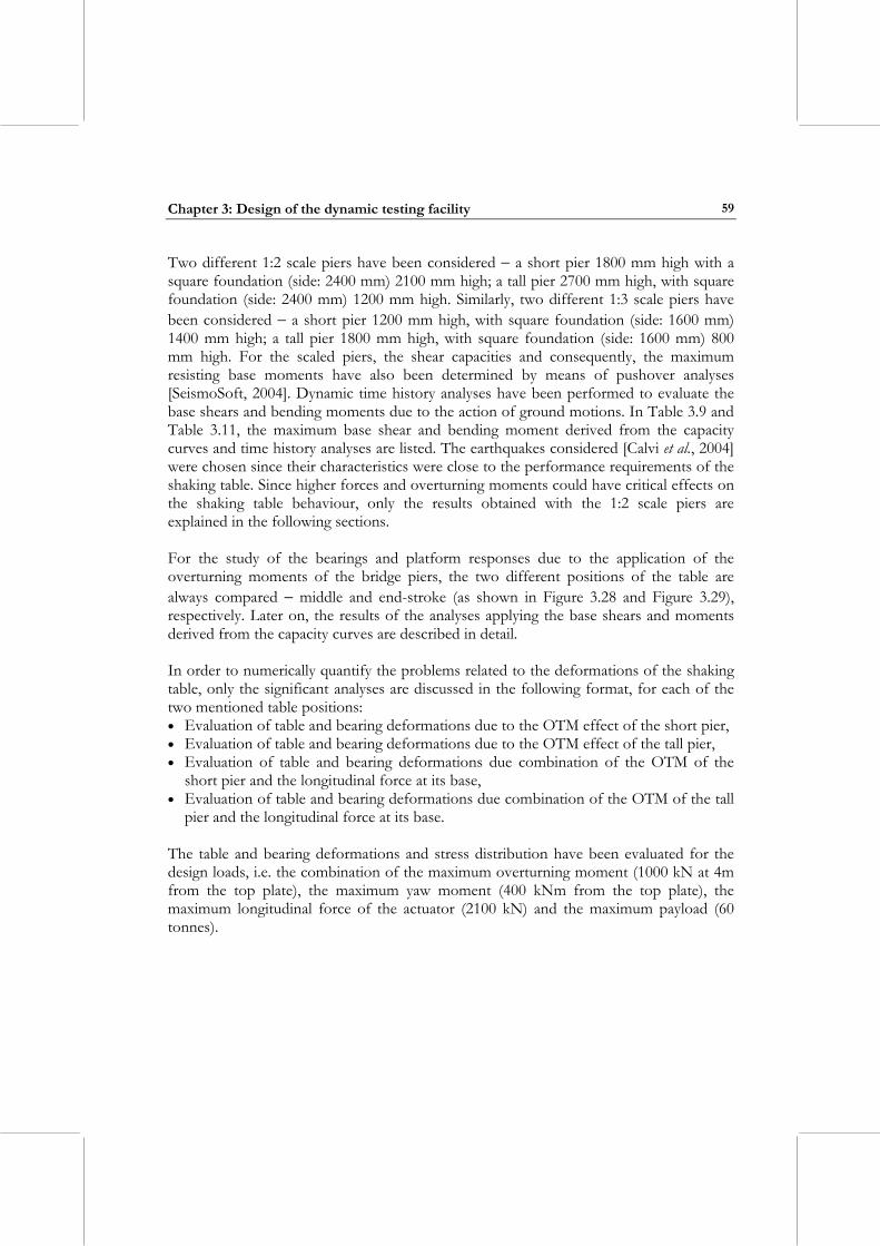
Chapter 3: Design of the dynamic testing facility
59
Two different 1:2 scale piers have been considered − a short pier 1800 mm high with a square foundation (side: 2400 mm) 2100 mm high; a tall pier 2700 mm high, with square foundation (side: 2400 mm) 1200 mm high. Similarly, two different 1:3 scale piers have been considered − a short pier 1200 mm high, with square foundation (side: 1600 mm) 1400 mm high; a tall pier 1800 mm high, with square foundation (side: 1600 mm) 800 mm high. For the scaled piers, the shear capacities and consequently, the maximum resisting base moments have also been determined by means of pushover analyses [SeismoSoft, 2004]. Dynamic time history analyses have been performed to evaluate the base shears and bending moments due to the action of ground motions. In Table 3.9 and Table 3.11, the maximum base shear and bending moment derived from the capacity curves and time history analyses are listed. The earthquakes considered [Calvi et al., 2004] were chosen since their characteristics were close to the performance requirements of the shaking table. Since higher forces and overturning moments could have critical effects on the shaking table behaviour, only the results obtained with the 1:2 scale piers are explained in the following sections. For the study of the bearings and platform responses due to the application of the overturning moments of the bridge piers, the two different positions of the table are always compared − middle and end-stroke (as shown in Figure 3.28 and Figure 3.29), respectively. Later on, the results of the analyses applying the base shears and moments derived from the capacity curves are described in detail. In order to numerically quantify the problems related to the deformations of the shaking table, only the significant analyses are discussed in the following format, for each of the two mentioned table positions: • Evaluation of table and bearing deformations due to the OTM effect of the short pier, • Evaluation of table and bearing deformations due to the OTM effect of the tall pier, • Evaluation of table and bearing deformations due combination of the OTM of the
short pier and the longitudinal force at its base, • Evaluation of table and bearing deformations due combination of the OTM of the tall
pier and the longitudinal force at its base. The table and bearing deformations and stress distribution have been evaluated for the design loads, i.e. the combination of the maximum overturning moment (1000 kN at 4m from the top plate), the maximum yaw moment (400 kNm from the top plate), the maximum longitudinal force of the actuator (2100 kN) and the maximum payload (60 tonnes).
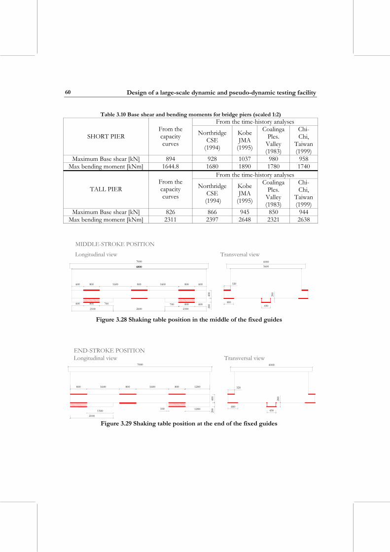
Design of a large-scale dynamic and pseudo-dynamic testing facility
60
Table 3.10 Base shear and bending moments for bridge piers (scaled 1:2) From the time-history analyses
SHORT PIER From the capacity curves
Northridge CSE
(1994)
Kobe JMA
(1995)
Coalinga Ples.
Valley (1983)
Chi-Chi,
Taiwan (1999)
Maximum Base shear [kN] 894 928 1037 980 958 Max bending moment [kNm] 1644.8 1680 1890 1780 1740
From the time-history analyses
TALL PIER From the capacity curves
Northridge CSE
(1994)
Kobe JMA
(1995)
Coalinga Ples.
Valley (1983)
Chi-Chi,
Taiwan (1999)
Maximum Base shear [kN] 826 866 945 850 944 Max bending moment [kNm] 2311 2397 2648 2321 2638
600 800 1600 800 1600 800 600
400
200
Longitudinal view
6800
40003600
430
200
320
MIDDLE-STROKE POSITION
7000
480
Transversal view
6800
2100 2600 2100
700600 700 600800 800
Figure 3.28 Shaking table position in the middle of the fixed guides
Transversal viewLongitudinal view4000
200
400
12001600800
7000
END-STROKE POSITION
800 1600 800
21001300
100 1200480
320
200
430
Figure 3.29 Shaking table position at the end of the fixed guides

Chapter 3: Design of the dynamic testing facility
61
Table 3.11 Base shear and bending moments for bridge piers (scaled 1:3) From the time-history analyses
SHORT PIER From the capacity curves
Northridge CSE
(1994)
Kobe JMA
(1995)
Coalinga Ples.
Valley (1983)
Chi-Chi, Taiwan (1999)
Maximum Base shear [kN] 397 381 422 452 434 Max bending moment [kNm] 487 460 511 546 493
From the time-history analyses
TALL PIER From the capacity curves
Northridge CSE
(1994)
Kobe JMA
(1995)
Coalinga Ples.
Valley (1983)
Chi-Chi, Taiwan (1999)
Maximum Base shear [kN] 367 373 419 392 415 Max bending moment [kNm] 685 680 780 715 773
Method To evaluate whether the proposed solution for table and hydrostatic bearings satisfy the design requirements, static analyses were performed. The overturning moment effects due to the 1:2 scale piers (Table 3.10) are studied considering the two critical situations of middle- and end-stroke positions. The combined effects due to the application of the maximum design overturning moment (4000 kNm at the top plate), maximum design yaw moment (400 kNm at the top plate) and the maximum dynamic longitudinal force (1700 kN) was considered. The results of the analyses performed could give quantitative evaluations of the system behaviour. It is clear that when the springs are in tension the results are not completely realistic since the viscous fluid cannot work in tension. It is also true that the simulation of the behaviour of the pressurized viscous fluid cannot simply be made by linear springs as has been carried out in the following analyses. A specific program is required to model the real behaviour of pressurized viscous fluid under static and dynamic excitations. As an approximation, cut-off elements, which work only in compression and not in tension, were used in some analyses. The effort implies longer time for computations since a very short time step for the load increase must be given to ensure the final convergence of the analysis. In the end, the results did not change significantly from the ones obtained with linear equivalent springs. Therefore, the final choice was to accept the results obtained from the analyses with equivalent springs as a good estimate in reasonable computational time.
3.6.3 Short pier: overturning moment effects The analysis is carried out considering the overturning moment caused by the pier yielding force and the foundation weight as applied loads. The results in terms of reactions and deformations of the bearings are summarized in Table 3.13 for the middle stroke position. The deformations of the hydrostatic bearings are computed knowing the hydrostatic stiffness of the pressurized viscous fluid (Table 3.3) and using the reactions, resulting from the analysis. The results show that the deformations are less than viscous
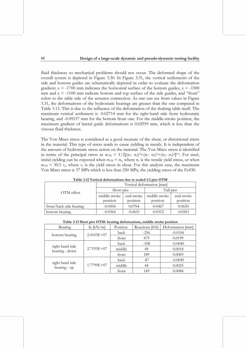
Design of a large-scale dynamic and pseudo-dynamic testing facility
62
fluid thickness so mechanical problems should not occur. The deformed shape of the overall system is depicted in Figure 3.30. In Figure 3.31, the vertical settlements of the side and bottom guides are schematically depicted in order to evaluate the deformation gradient: z = -1700 mm indicates the horizontal surface of the bottom guides, z = -1500 mm and z = -1100 mm indicate bottom and top surface of the side guides, and “front” refers to the table side of the actuator connection. As one can see from values in Figure 3.31, the deformations of the hydrostatic bearings are greater than the one computed in Table 3.13. This is due to the influence of the deformation of the shaking table itself. The maximum vertical settlement is -0.02714 mm for the right-hand side front hydrostatic bearing, and -0.09157 mm for the bottom front one. For the middle-stroke position, the maximum gradient of lateral guide deformations is 0.02959 mm, which is less than the viscous fluid thickness. The Von Mises stress is considered as a good measure of the shear, or distortional stress in the material. This type of stress tends to cause yielding in metals. It is independent of the amount of hydrostatic stress action on the material. The Von Mises stress is identified in terms of the principal stress as σVM = 1/2[(σ1- σ2)2+(σ1- σ3)2+(σ2- σ3)2]0.5. For steel, initial yielding can be expected when σVM = σy, where σy is the tensile yield stress, or when σVM = 30.5 τy, where τy is the yield stress in shear. For this analysis case, the maximum Von Mises stress is 37 MPa which is less than 250 MPa, the yielding stress of the Fe430.
Table 3.12 Vertical deformations due to scaled 1:2 pier OTM Vertical deformation [mm]
Short pier Tall pier OTM effect middle-stroke
position end-stroke position
middle-stroke position
end-stroke position
front/back side bearing -0.0504 0.0704 -0.0467 0.0650 bottom bearing -0.0364 -0.0651 -0.0312 -0.0561
Table 3.13 Short pier OTM: bearing deformations, middle stroke position
Bearing K [kN/m] Position Reactions [kN] Deformation [mm] back -256 -0.0106 bottom bearing 2.4103E+07 front 479 0.0199 back -108 -0.0040
middle 49 0.0018 right hand side bearing - down 2.7193E+07
front 189 0.0069 back -87 -0.0049
middle 44 0.0025 right hand side
bearing - up 1.7799E+07 front 149 0.0084
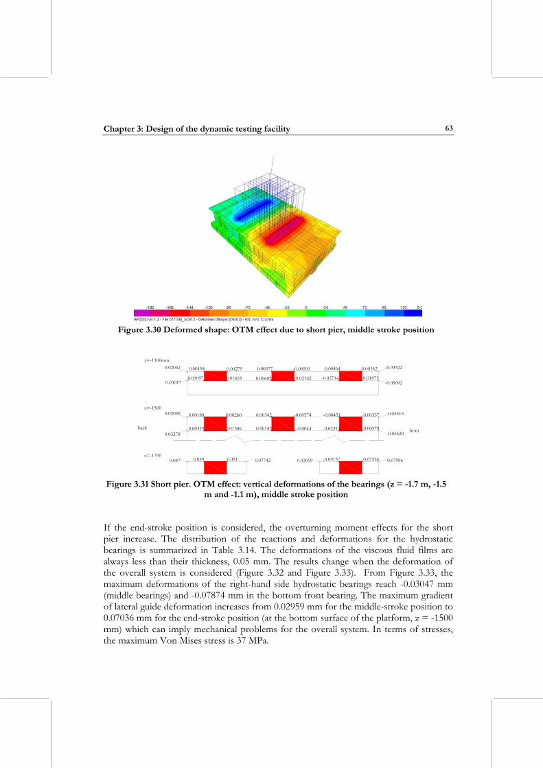
Chapter 3: Design of the dynamic testing facility
63
Figure 3.30 Deformed shape: OTM effect due to short pier, middle stroke position
front
z=-1700
z=-1500
z=-1100mm
back
-0.05092
-0.03522
-0.01873-0.02714-0.021620.006820.016180.01097
-0.00342-0.00464-0.005910.003770.002790.001940.02062
0.03017
0.02059
0.032780.00319 0.01386 0.00145 -0.0044 -0.02313 -0.00579
-0.00337-0.00451-0.005740.003420.002600.00189
-0.05620
-0.03515
0.0510.039 0.077420.047 0.02059 -0.09157 -0.07534 -0.07996
Figure 3.31 Short pier. OTM effect: vertical deformations of the bearings (z = -1.7 m, -1.5
m and -1.1 m), middle stroke position
If the end-stroke position is considered, the overturning moment effects for the short pier increase. The distribution of the reactions and deformations for the hydrostatic bearings is summarized in Table 3.14. The deformations of the viscous fluid films are always less than their thickness, 0.05 mm. The results change when the deformation of the overall system is considered (Figure 3.32 and Figure 3.33). From Figure 3.33, the maximum deformations of the right-hand side hydrostatic bearings reach -0.03047 mm (middle bearings) and -0.07874 mm in the bottom front bearing. The maximum gradient of lateral guide deformation increases from 0.02959 mm for the middle-stroke position to 0.07036 mm for the end-stroke position (at the bottom surface of the platform, z = -1500 mm) which can imply mechanical problems for the overall system. In terms of stresses, the maximum Von Mises stress is 37 MPa.
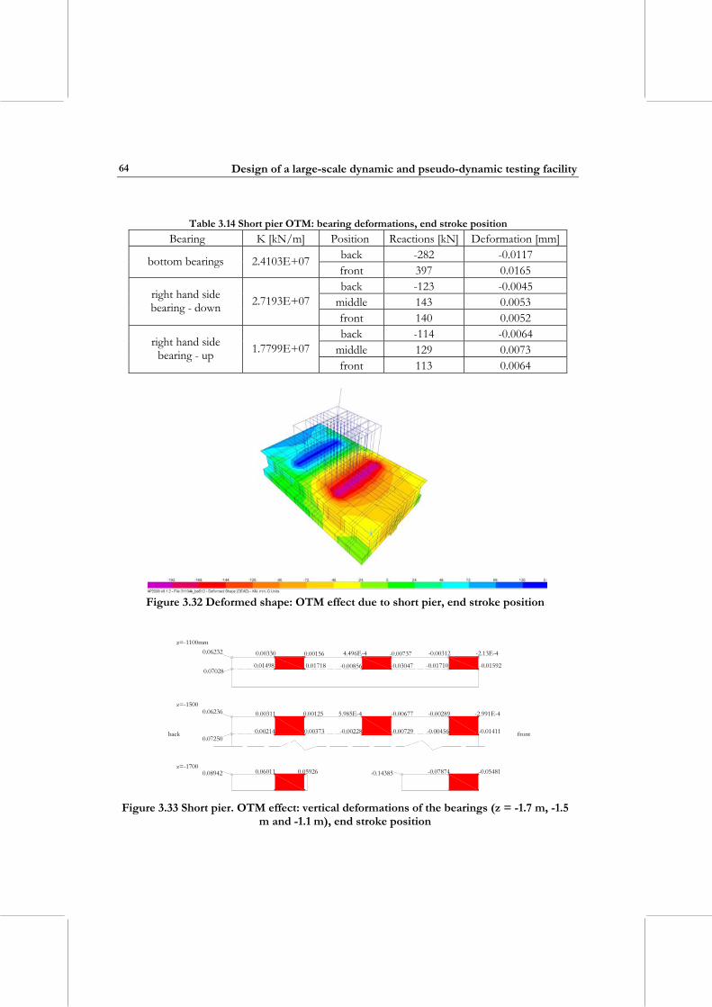
Design of a large-scale dynamic and pseudo-dynamic testing facility
64
Table 3.14 Short pier OTM: bearing deformations, end stroke position
Bearing K [kN/m] Position Reactions [kN] Deformation [mm] back -282 -0.0117 bottom bearings 2.4103E+07 front 397 0.0165 back -123 -0.0045
middle 143 0.0053 right hand side bearing - down 2.7193E+07
front 140 0.0052 back -114 -0.0064
middle 129 0.0073 right hand side
bearing - up 1.7799E+07 front 113 0.0064
Figure 3.32 Deformed shape: OTM effect due to short pier, end stroke position
-0.05481-0.07874-0.143850.08942 0.06011 0.05926
0.00311 0.00125 5.985E-4 -0.00677 -0.00289 -2.991E-4
-0.01411-0.00456-0.00729-0.002280.003730.002140.07250
0.06236
0.07028
0.06232 0.00330 0.00156 4.496E-4 -0.00737 -0.00312 -2.13E-4
0.01498 0.01718 -0.00856 -0.03047 -0.01710 -0.01592
back
z=-1100mm
z=-1500
z=-1700
front
Figure 3.33 Short pier. OTM effect: vertical deformations of the bearings (z = -1.7 m, -1.5
m and -1.1 m), end stroke position
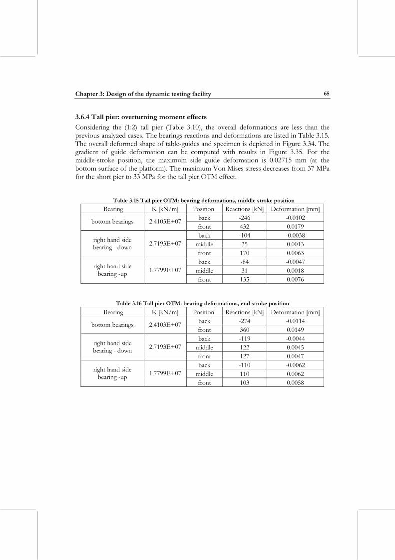
Chapter 3: Design of the dynamic testing facility
65
3.6.4 Tall pier: overturning moment effects Considering the (1:2) tall pier (Table 3.10), the overall deformations are less than the previous analyzed cases. The bearings reactions and deformations are listed in Table 3.15. The overall deformed shape of table-guides and specimen is depicted in Figure 3.34. The gradient of guide deformation can be computed with results in Figure 3.35. For the middle-stroke position, the maximum side guide deformation is 0.02715 mm (at the bottom surface of the platform). The maximum Von Mises stress decreases from 37 MPa for the short pier to 33 MPa for the tall pier OTM effect.
Table 3.15 Tall pier OTM: bearing deformations, middle stroke position Bearing K [kN/m] Position Reactions [kN] Deformation [mm]
back -246 -0.0102 bottom bearings 2.4103E+07 front 432 0.0179 back -104 -0.0038
middle 35 0.0013 right hand side bearing - down 2.7193E+07
front 170 0.0063 back -84 -0.0047
middle 31 0.0018 right hand side
bearing -up 1.7799E+07 front 135 0.0076
Table 3.16 Tall pier OTM: bearing deformations, end stroke position Bearing K [kN/m] Position Reactions [kN] Deformation [mm]
back -274 -0.0114 bottom bearings 2.4103E+07 front 360 0.0149 back -119 -0.0044
middle 122 0.0045 right hand side bearing - down 2.7193E+07
front 127 0.0047 back -110 -0.0062
middle 110 0.0062 right hand side
bearing -up 1.7799E+07 front 103 0.0058
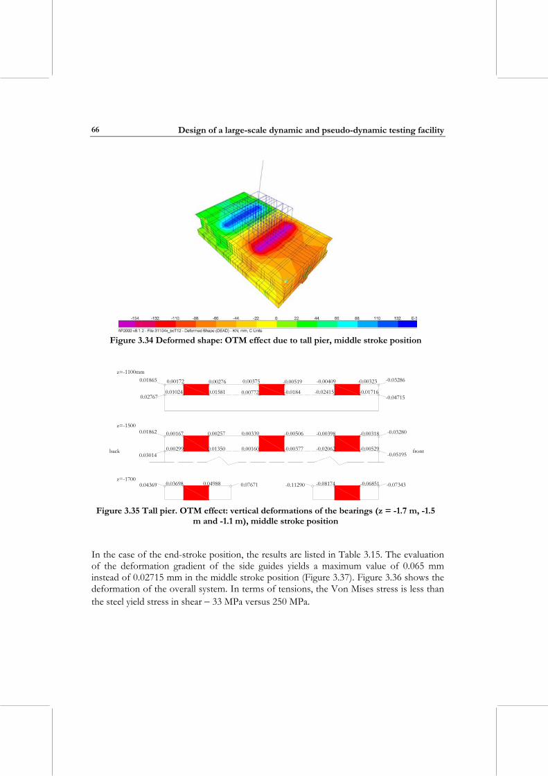
Design of a large-scale dynamic and pseudo-dynamic testing facility
66
Figure 3.34 Deformed shape: OTM effect due to tall pier, middle stroke position
0.00375 -0.00519 -0.00409 -0.00323
0.01024 0.01581 0.00772 -0.0184 -0.02415 -0.01716
-0.03286
-0.04715
back
z=-1100mm
z=-1500
z=-1700
front
-0.07343-0.06851-0.08174-0.112900.04369 0.076710.03698 0.04988
-0.03280
-0.05195
0.00167 0.00257 0.00339 -0.00506 -0.00398 -0.00318
-0.00529-0.02062-0.003770.001600.013500.002990.03014
0.01862
0.02767
0.01865 0.00172 0.00276
Figure 3.35 Tall pier. OTM effect: vertical deformations of the bearings (z = -1.7 m, -1.5
m and -1.1 m), middle stroke position
In the case of the end-stroke position, the results are listed in Table 3.15. The evaluation of the deformation gradient of the side guides yields a maximum value of 0.065 mm instead of 0.02715 mm in the middle stroke position (Figure 3.37). Figure 3.36 shows the deformation of the overall system. In terms of tensions, the Von Mises stress is less than the steel yield stress in shear − 33 MPa versus 250 MPa.
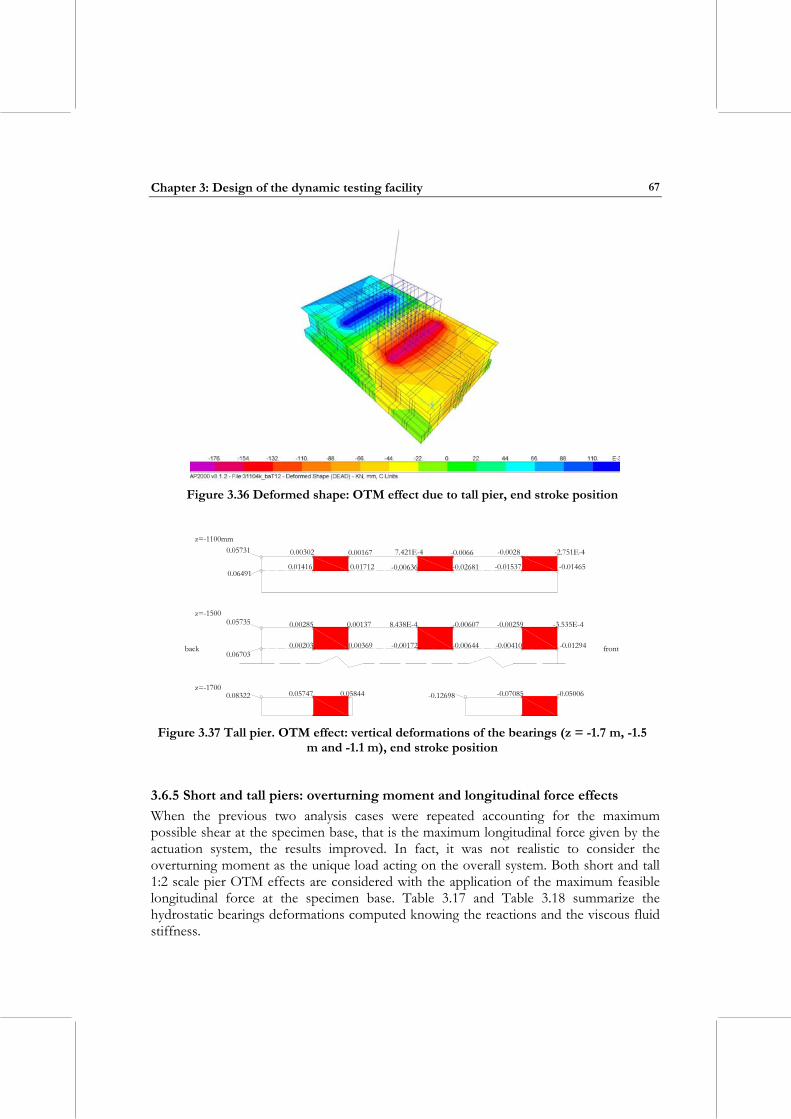
Chapter 3: Design of the dynamic testing facility
67
Figure 3.36 Deformed shape: OTM effect due to tall pier, end stroke position
0.001370.00285
0.058440.057470.08322 -0.12698 -0.07085 -0.05006
front
z=-1700
z=-1500
z=-1100mm
back
-0.01465-0.01537-0.02681-0.006360.017120.01416
-2.751E-4-0.0028-0.00667.421E-40.001670.003020.05731
0.06491
0.05735
0.067030.00203 0.00369 -0.00172 -0.00644 -0.00410 -0.01294
-3.535E-4-0.00259-0.006078.438E-4
Figure 3.37 Tall pier. OTM effect: vertical deformations of the bearings (z = -1.7 m, -1.5
m and -1.1 m), end stroke position
3.6.5 Short and tall piers: overturning moment and longitudinal force effects When the previous two analysis cases were repeated accounting for the maximum possible shear at the specimen base, that is the maximum longitudinal force given by the actuation system, the results improved. In fact, it was not realistic to consider the overturning moment as the unique load acting on the overall system. Both short and tall 1:2 scale pier OTM effects are considered with the application of the maximum feasible longitudinal force at the specimen base. Table 3.17 and Table 3.18 summarize the hydrostatic bearings deformations computed knowing the reactions and the viscous fluid stiffness.
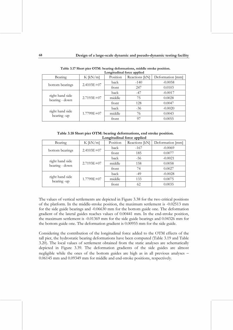
Design of a large-scale dynamic and pseudo-dynamic testing facility
68
Table 3.17 Short pier OTM: bearing deformations, middle stroke position. Longitudinal force applied
Bearing K [kN/m] Position Reactions [kN] Deformation [mm] back -140 -0.0058 bottom bearings 2.4103E+07 front 247 0.0103 back -47 -0.0017
middle 75 0.0028 right hand side bearing - down 2.7193E+07
front 128 0.0047 back -36 -0.0020
middle 76 0.0043 right hand side bearing -up 1.7799E+07
front 97 0.0055
Table 3.18 Short pier OTM: bearing deformations, end stroke position. Longitudinal force applied
Bearing K [kN/m] Position Reactions [kN] Deformation [mm] back -167 -0.0069 bottom bearings 2.4103E+07 front 185 0.0077 back -56 -0.0021
middle 158 0.0058 right hand side bearing - down 2.7193E+07
front 74 0.0027 back -49 -0.0028
middle 133 0.0075 right hand side bearing -up 1.7799E+07
front 62 0.0035 The values of vertical settlements are depicted in Figure 3.38 for the two critical positions of the platform. In the middle-stroke position, the maximum settlement is -0.02513 mm for the side guide bearings and -0.06630 mm for the bottom guide one. The deformation gradient of the lateral guides reaches values of 0.00441 mm. In the end-stroke position, the maximum settlement is -0.01369 mm for the side guide bearings and 0.04326 mm for the bottom guide one. The deformation gradient is 0.00955 mm for the side guide. Considering the contribution of the longitudinal force added to the OTM effects of the tall pier, the hydrostatic bearing deformations have been computed (Table 3.19 and Table 3.20). The local values of settlement obtained from the static analyses are schematically depicted in Figure 3.39. The deformation gradients of the side guides are almost negligible while the ones of the bottom guides are high as in all previous analyses − 0.06145 mm and 0.09349 mm for middle and end-stroke positions, respectively.
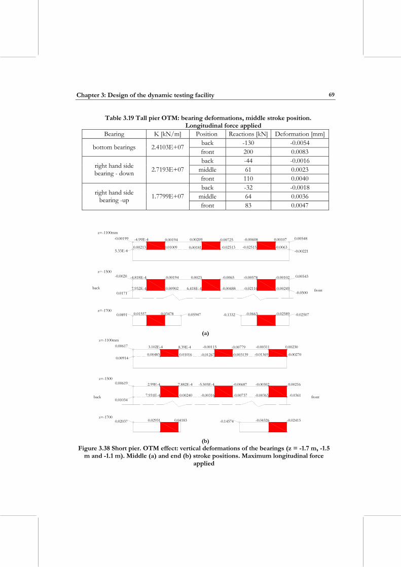
Chapter 3: Design of the dynamic testing facility
69
Table 3.19 Tall pier OTM: bearing deformations, middle stroke position. Longitudinal force applied
Bearing K [kN/m] Position Reactions [kN] Deformation [mm] back -130 -0.0054 bottom bearings 2.4103E+07 front 200 0.0083 back -44 -0.0016
middle 61 0.0023 right hand side bearing - down 2.7193E+07
front 110 0.0040 back -32 -0.0018
middle 64 0.0036 right hand side bearing -up 1.7799E+07
front 83 0.0047
-0.02507-0.02589-0.0663-0.13320.0891 0.059470.01557 0.03478
0.00543
-0.0500
-4.818E-4 0.00194 0.0023 -0.0065 -0.00578 -0.00102
-0.00249-0.02116-0.004886.418E-40.009027.932E-40.0171
-0.0020
5.33E-4
-0.00199 -4.99E-4 0.00194 0.00209 -0.00725 -0.00608 0.00107
0.00213 0.01009 0.00181 -0.02513 -0.02513 -0.0063
0.00548
-0.00221
back
z=-1100mm
z=-1500
z=-1700
front
(a)
front
z=-1700
z=-1500
z=-1100mm
back
-0.00270-0.01369-0.003139-0.012670.010160.00483
0.00230-0.00311-0.00779-0.001158.39E-43.102E-40.00617
0.00914
0.00619
0.010347.931E-4 0.00240 -0.00316 -0.00737 -0.00365 -0.0361
0.00216-0.00302-0.00687-5.505E-47.882E-42.99E-4
0.041830.029310.02037 -0.14574 -0.04326 -0.02413
(b)
Figure 3.38 Short pier. OTM effect: vertical deformations of the bearings (z = -1.7 m, -1.5 m and -1.1 m). Middle (a) and end (b) stroke positions. Maximum longitudinal force
applied
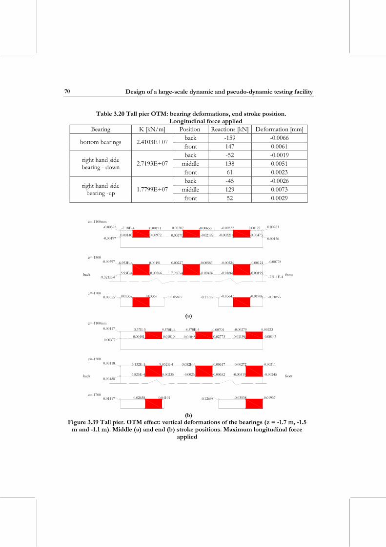
Design of a large-scale dynamic and pseudo-dynamic testing facility
70
Table 3.20 Tall pier OTM: bearing deformations, end stroke position. Longitudinal force applied
Bearing K [kN/m] Position Reactions [kN] Deformation [mm] back -159 -0.0066 bottom bearings 2.4103E+07 front 147 0.0061 back -52 -0.0019
middle 138 0.0051 right hand side bearing - down 2.7193E+07
front 61 0.0023 back -45 -0.0026
middle 129 0.0073 right hand side bearing -up 1.7799E+07
front 52 0.0029
front
z=-1700
z=-1500
z=-1100mm
back
0.00156
0.00783
-0.00473-0.002214-0.021920.002710.009720.00140
0.00127-0.00552-0.006530.002070.00191-7.18E-4-0.00395
-0.00197
-0.00397
-9.321E-45.93E-4 0.00866 7.96E-4 -0.00476 -0.01864 -0.00199
-0.00121-0.00524-0.005830.002270.00191-6.953E-4
-7.511E-4
-0.00778
0.033570.01352 0.058750.00555 -0.11792 -0.05647 -0.01906 -0.01853
(a)
-0.01937-0.03538-0.126980.01417 0.02658 0.04101
3.132E-5 9.052E-4 -3.052E-4 -0.00617 -0.00272 -0.00211
-0.00245-0.00319-0.00652-0.00260.002356.825E-40.00488
0.00118
0.00377
0.00117 3.37E-5 9.578E-4 -8.578E-4 -0.00701 -0.00279 0.00223
0.00401 0.01010 -0.01048 -0.02773 -0.01196 -0.00143
back
z=-1100mm
z=-1500
z=-1700
front
(b)
Figure 3.39 Tall pier. OTM effect: vertical deformations of the bearings (z = -1.7 m, -1.5 m and -1.1 m). Middle (a) and end (b) stroke positions. Maximum longitudinal force
applied
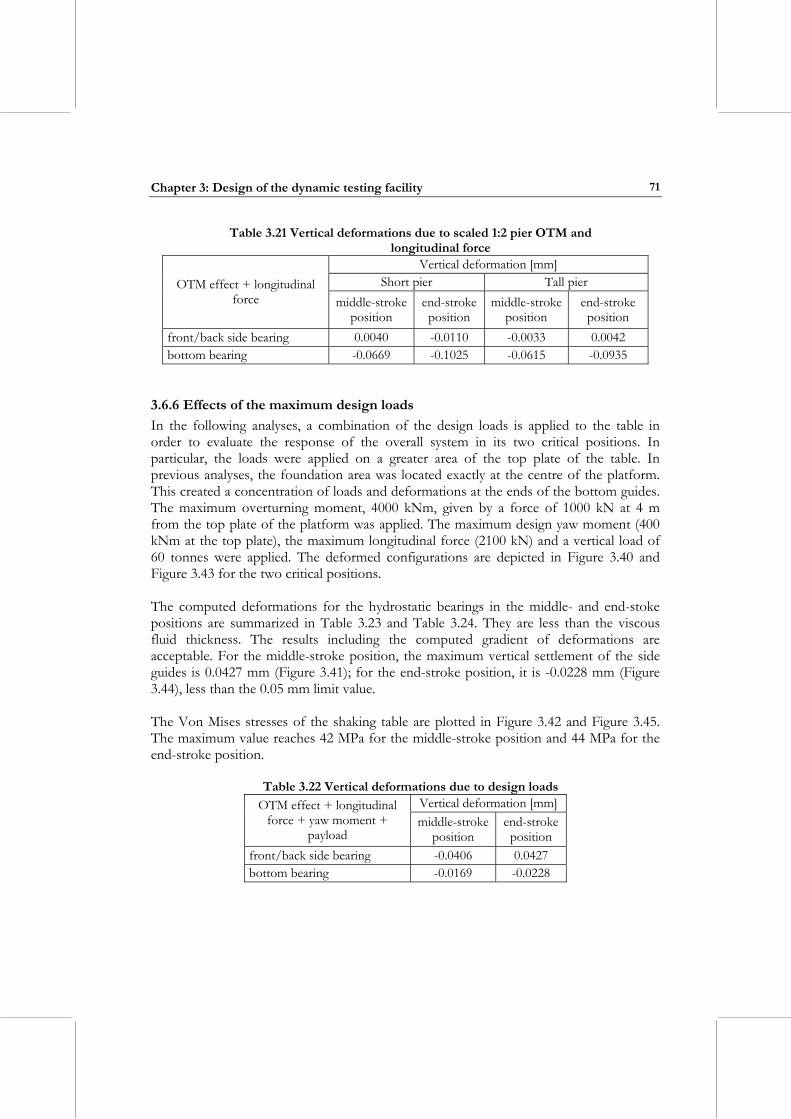
Chapter 3: Design of the dynamic testing facility
71
Table 3.21 Vertical deformations due to scaled 1:2 pier OTM and longitudinal force
Vertical deformation [mm] Short pier Tall pier OTM effect + longitudinal
force middle-stroke position
end-stroke position
middle-stroke position
end-stroke position
front/back side bearing 0.0040 -0.0110 -0.0033 0.0042 bottom bearing -0.0669 -0.1025 -0.0615 -0.0935
3.6.6 Effects of the maximum design loads In the following analyses, a combination of the design loads is applied to the table in order to evaluate the response of the overall system in its two critical positions. In particular, the loads were applied on a greater area of the top plate of the table. In previous analyses, the foundation area was located exactly at the centre of the platform. This created a concentration of loads and deformations at the ends of the bottom guides. The maximum overturning moment, 4000 kNm, given by a force of 1000 kN at 4 m from the top plate of the platform was applied. The maximum design yaw moment (400 kNm at the top plate), the maximum longitudinal force (2100 kN) and a vertical load of 60 tonnes were applied. The deformed configurations are depicted in Figure 3.40 and Figure 3.43 for the two critical positions. The computed deformations for the hydrostatic bearings in the middle- and end-stoke positions are summarized in Table 3.23 and Table 3.24. They are less than the viscous fluid thickness. The results including the computed gradient of deformations are acceptable. For the middle-stroke position, the maximum vertical settlement of the side guides is 0.0427 mm (Figure 3.41); for the end-stroke position, it is -0.0228 mm (Figure 3.44), less than the 0.05 mm limit value. The Von Mises stresses of the shaking table are plotted in Figure 3.42 and Figure 3.45. The maximum value reaches 42 MPa for the middle-stroke position and 44 MPa for the end-stroke position.
Table 3.22 Vertical deformations due to design loads Vertical deformation [mm]OTM effect + longitudinal
force + yaw moment + payload
middle-stroke position
end-stroke position
front/back side bearing -0.0406 0.0427 bottom bearing -0.0169 -0.0228
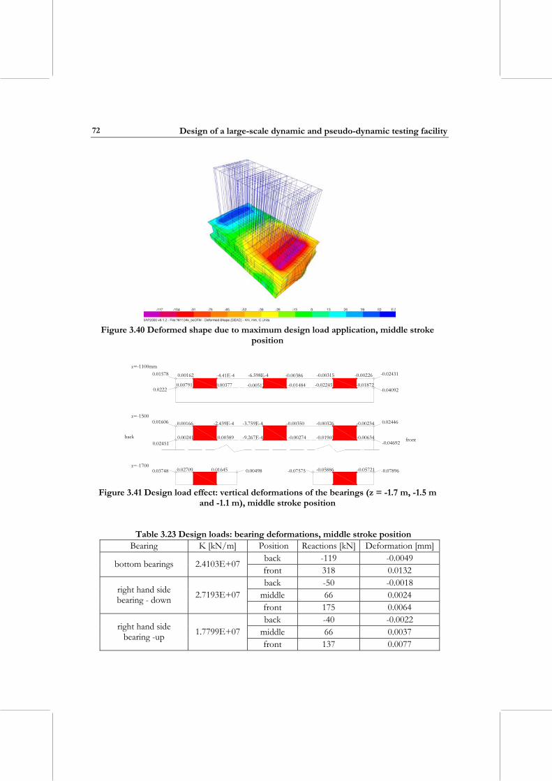
Design of a large-scale dynamic and pseudo-dynamic testing facility
72
Figure 3.40 Deformed shape due to maximum design load application, middle stroke
position
-0.04092
-0.02431
-0.01872-0.02245-0.01484-0.005120.003770.00791
-0.00226-0.00315-0.00386-6.598E-4-4.41E-40.001620.01578
0.0222
0.01606
0.024510.00241 0.00389 -9.267E-4 -0.00274 -0.01969 -0.00634
-0.00234-0.00326-0.00350-3.759E-4-2.439E-40.00166
-0.04692
0.02446
0.016450.02709 0.004980.03748 -0.07575 -0.05886 -0.05721 -0.07896
front
z=-1700
z=-1500
z=-1100mm
back
Figure 3.41 Design load effect: vertical deformations of the bearings (z = -1.7 m, -1.5 m
and -1.1 m), middle stroke position
Table 3.23 Design loads: bearing deformations, middle stroke position Bearing K [kN/m] Position Reactions [kN] Deformation [mm]
back -119 -0.0049 bottom bearings 2.4103E+07 front 318 0.0132 back -50 -0.0018
middle 66 0.0024 right hand side bearing - down 2.7193E+07
front 175 0.0064 back -40 -0.0022
middle 66 0.0037 right hand side bearing -up 1.7799E+07
front 137 0.0077
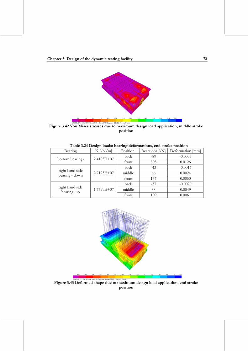
Chapter 3: Design of the dynamic testing facility
73
Figure 3.42 Von Mises stresses due to maximum design load application, middle stroke
position
Table 3.24 Design loads: bearing deformations, end stroke position
Bearing K [kN/m] Position Reactions [kN] Deformation [mm] back -89 -0.0037 bottom bearings 2.4103E+07 front 303 0.0126 back -43 -0.0016
middle 66 0.0024 right hand side bearing - down 2.7193E+07
front 137 0.0050 back -37 -0.0020
middle 88 0.0049 right hand side bearing -up 1.7799E+07
front 109 0.0061
Figure 3.43 Deformed shape due to maximum design load application, end stroke
position
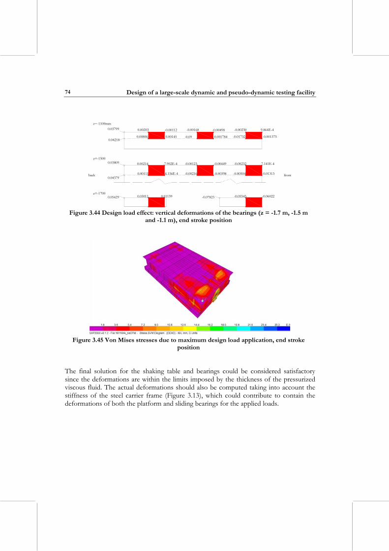
Design of a large-scale dynamic and pseudo-dynamic testing facility
74
-0.06022-0.05543-0.078230.05429 0.03011 0.01159
0.00214 -7.902E-4 -0.00123 -0.00449 -0.00232 7.141E-4
-0.01313-0.00504-0.00398-0.002164.156E-40.001110.04379
0.03809
0.04218
0.03799 0.00203 -0.00112 -0.00168 -0.00498 -0.00230 9.864E-4
0.00806 0.00145 -0.09 -0.001784 -0.01732 -0.001375
back
z=-1100mm
z=-1500
z=-1700
front
Figure 3.44 Design load effect: vertical deformations of the bearings (z = -1.7 m, -1.5 m
and -1.1 m), end stroke position
Figure 3.45 Von Mises stresses due to maximum design load application, end stroke
position
The final solution for the shaking table and bearings could be considered satisfactory since the deformations are within the limits imposed by the thickness of the pressurized viscous fluid. The actual deformations should also be computed taking into account the stiffness of the steel carrier frame (Figure 3.13), which could contribute to contain the deformations of both the platform and sliding bearings for the applied loads.
CHAPTER 4: DESIGN OF THE PSEUDO-DYNAMIC TESTING FACILITY
This chapter describes the design of the pseudo-dynamic (PsD) testing facility at the EUCENTRE laboratory. The main issues relevant for the design phase are briefly introduced. The structural configuration of both the strong floor and the reaction walls is given. The optimization that led to the final configuration – for both the strong floor and reaction walls – of the testing apparatus is described in the section related to the stiffness evaluation of the PsD apparatus. The design of the post-tensioning system is then illustrated. Finally, a description of the design of the foundation system is given.
4.1 RELEVANT ISSUES FOR THE DESIGN OF THE PSD FACILITY In some circumstances, it may be essential to test at full-scale, either because testing at a reduced scale would be too restrictive in terms of the types of materials that could be used or because construction of a small model would be too difficult. In these circumstances, shaking tables are not likely to be appropriate for most structures. On the other hand, pseudo-dynamic test rigs allow full-scale specimens to be tested, although not with actual inertia forces. A reaction wall is a large, very stiff wall that is used to provide support for actuators that are then used to deform large or life-size structures. Such a facility can be used to perform static or cyclic tests of large structures, but it is also possible to use a technique called pseudo-dynamic testing to simulate earthquake loading of full-scale structures. The performance characteristics of a PsD testing facility should allow testing full-scale structures such as bridge piers, multi storey reinforced concrete and/or masonry buildings. A few important issues related to a PsD facility’s performance are enlisted in the following. The optimum performance of the testing facility is influenced by each one of the following points that are, in turn, strongly correlated: • The dimensions of the strong floor and walls are a limitation to the type of tests. • The construction technology affects the high performance characteristics required for
the facility. In fact, one can chose a classical technology such as cast in-situ concrete for walls and floor. An alternative technology could be to assemble precast concrete blocks. In this case, a particular technology must be selected for the steel reinforcement, as well. For example, post-tensioned steel cables to assemble the whole precast structure, absorb the tensile stresses in the concrete and maintain certain stress levels despite tension drops, could be an alternative.
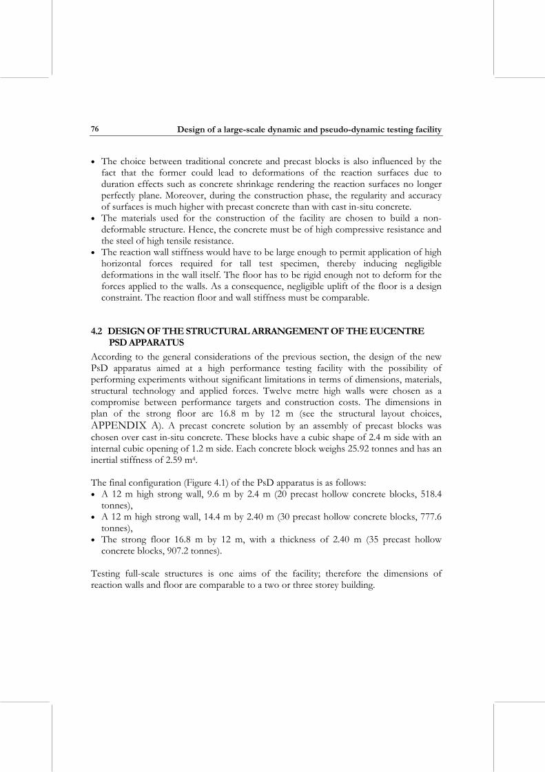
Design of a large-scale dynamic and pseudo-dynamic testing facility
76
• The choice between traditional concrete and precast blocks is also influenced by the fact that the former could lead to deformations of the reaction surfaces due to duration effects such as concrete shrinkage rendering the reaction surfaces no longer perfectly plane. Moreover, during the construction phase, the regularity and accuracy of surfaces is much higher with precast concrete than with cast in-situ concrete.
• The materials used for the construction of the facility are chosen to build a non-deformable structure. Hence, the concrete must be of high compressive resistance and the steel of high tensile resistance.
• The reaction wall stiffness would have to be large enough to permit application of high horizontal forces required for tall test specimen, thereby inducing negligible deformations in the wall itself. The floor has to be rigid enough not to deform for the forces applied to the walls. As a consequence, negligible uplift of the floor is a design constraint. The reaction floor and wall stiffness must be comparable.
4.2 DESIGN OF THE STRUCTURAL ARRANGEMENT OF THE EUCENTRE PSD APPARATUS
According to the general considerations of the previous section, the design of the new PsD apparatus aimed at a high performance testing facility with the possibility of performing experiments without significant limitations in terms of dimensions, materials, structural technology and applied forces. Twelve metre high walls were chosen as a compromise between performance targets and construction costs. The dimensions in plan of the strong floor are 16.8 m by 12 m (see the structural layout choices, APPENDIX A). A precast concrete solution by an assembly of precast blocks was chosen over cast in-situ concrete. These blocks have a cubic shape of 2.4 m side with an internal cubic opening of 1.2 m side. Each concrete block weighs 25.92 tonnes and has an inertial stiffness of 2.59 m4. The final configuration (Figure 4.1) of the PsD apparatus is as follows: • A 12 m high strong wall, 9.6 m by 2.4 m (20 precast hollow concrete blocks, 518.4
tonnes), • A 12 m high strong wall, 14.4 m by 2.40 m (30 precast hollow concrete blocks, 777.6
tonnes), • The strong floor 16.8 m by 12 m, with a thickness of 2.40 m (35 precast hollow
concrete blocks, 907.2 tonnes). Testing full-scale structures is one aims of the facility; therefore the dimensions of reaction walls and floor are comparable to a two or three storey building.
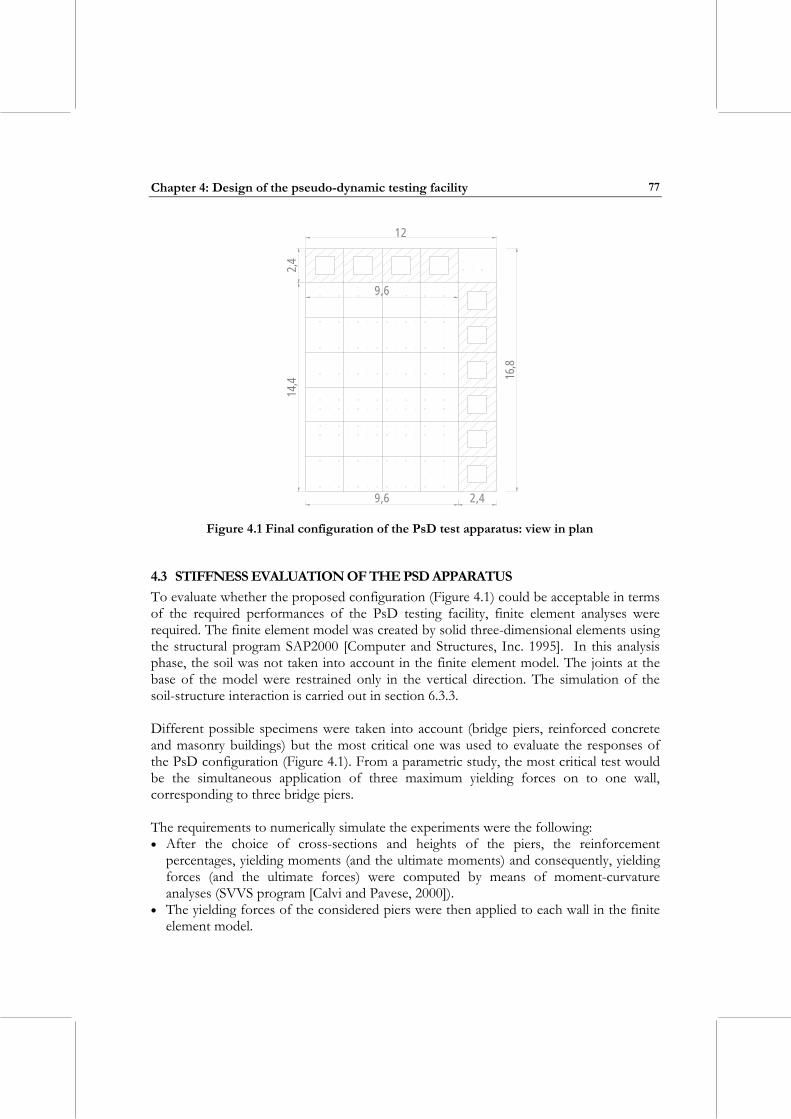
Chapter 4: Design of the pseudo-dynamic testing facility
77
12
9,62,4
16,8
14,4
9,6 2,4
Figure 4.1 Final configuration of the PsD test apparatus: view in plan
4.3 STIFFNESS EVALUATION OF THE PSD APPARATUS To evaluate whether the proposed configuration (Figure 4.1) could be acceptable in terms of the required performances of the PsD testing facility, finite element analyses were required. The finite element model was created by solid three-dimensional elements using the structural program SAP2000 [Computer and Structures, Inc. 1995]. In this analysis phase, the soil was not taken into account in the finite element model. The joints at the base of the model were restrained only in the vertical direction. The simulation of the soil-structure interaction is carried out in section 6.3.3. Different possible specimens were taken into account (bridge piers, reinforced concrete and masonry buildings) but the most critical one was used to evaluate the responses of the PsD configuration (Figure 4.1). From a parametric study, the most critical test would be the simultaneous application of three maximum yielding forces on to one wall, corresponding to three bridge piers. The requirements to numerically simulate the experiments were the following: • After the choice of cross-sections and heights of the piers, the reinforcement
percentages, yielding moments (and the ultimate moments) and consequently, yielding forces (and the ultimate forces) were computed by means of moment-curvature analyses (SVVS program [Calvi and Pavese, 2000]).
• The yielding forces of the considered piers were then applied to each wall in the finite element model.
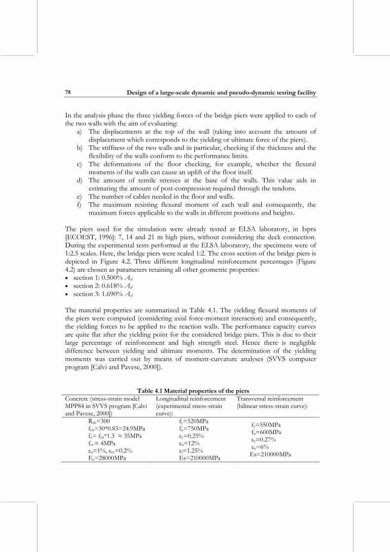
Design of a large-scale dynamic and pseudo-dynamic testing facility
78
In the analysis phase the three yielding forces of the bridge piers were applied to each of the two walls with the aim of evaluating:
a) The displacements at the top of the wall (taking into account the amount of displacement which corresponds to the yielding or ultimate force of the piers).
b) The stiffness of the two walls and in particular, checking if the thickness and the flexibility of the walls conform to the performance limits.
c) The deformations of the floor checking, for example, whether the flexural moments of the walls can cause an uplift of the floor itself.
d) The amount of tensile stresses at the base of the walls. This value aids in estimating the amount of post-compression required through the tendons.
e) The number of cables needed in the floor and walls. f) The maximum resisting flexural moment of each wall and consequently, the
maximum forces applicable to the walls in different positions and heights. The piers used for the simulation were already tested at ELSA laboratory, in Ispra [ECOEST, 1996]: 7, 14 and 21 m high piers, without considering the deck connection. During the experimental tests performed at the ELSA laboratory, the specimens were of 1:2.5 scales. Here, the bridge piers were scaled 1:2. The cross section of the bridge piers is depicted in Figure 4.2. Three different longitudinal reinforcement percentages (Figure 4.2) are chosen as parameters retaining all other geometric properties: • section 1: 0.500% Asl • section 2: 0.618% Asl • section 3: 1.690% Asl The material properties are summarized in Table 4.1. The yielding flexural moments of the piers were computed (considering axial force-moment interaction) and consequently, the yielding forces to be applied to the reaction walls. The performance capacity curves are quite flat after the yielding point for the considered bridge piers. This is due to their large percentage of reinforcement and high strength steel. Hence there is negligible difference between yielding and ultimate moments. The determination of the yielding moments was carried out by means of moment-curvature analyses (SVVS computer program [Calvi and Pavese, 2000]).
Table 4.1 Material properties of the piers Concrete (stress-strain model MPP84 in SVVS program [Calvi and Pavese, 2000])
Longitudinal reinforcement (experimental stress-strain curve):
Transversal reinforcement (bilinear stress-strain curve):
Rck=300 fck=30*0.83=24.9MPa fc= fck*1.3 ≈ 35MPa fct ≈ 4MPa εu=1%, εcc=0.2% Ec=28000MPa
fy=520MPa fu=750MPa εy=0.25% εu=12% εi=1.25% Es=210000MPa
fy=550MPa fu=600MPa εy=0.27% εu=6% Es=210000MPa
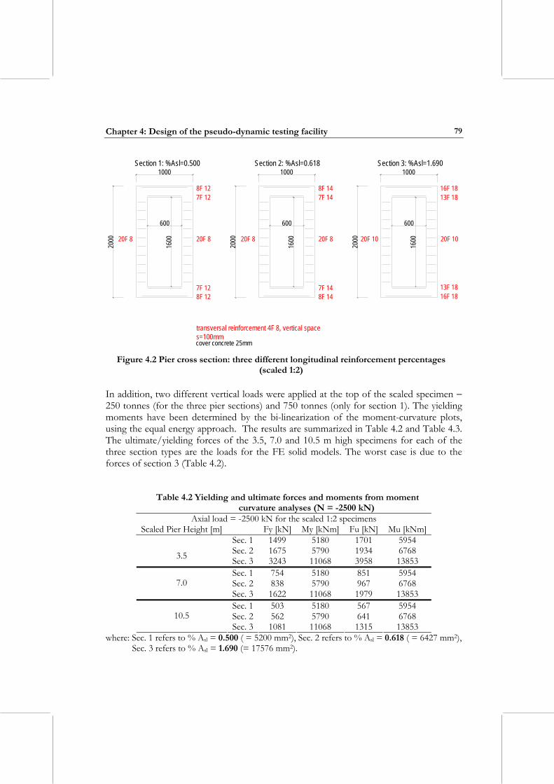
Chapter 4: Design of the pseudo-dynamic testing facility
79
8F 127F 12
7F 128F 12
1000
2000
1600
600
cover concrete 25mm
20F 820F 8
Section 1: %Asl=0.500
20F 8 20F 8
1600
2000
8F 147F 14
7F 14
600
Section 2: %Asl=0.6181000
8F 14
2000
1600 20F 1020F 10
13F 18
600
Section 3: %Asl=1.6901000
16F 18
16F 1813F 18
transversal reinforcement 4F 8, vertical space s=100mm
Figure 4.2 Pier cross section: three different longitudinal reinforcement percentages (scaled 1:2)
In addition, two different vertical loads were applied at the top of the scaled specimen − 250 tonnes (for the three pier sections) and 750 tonnes (only for section 1). The yielding moments have been determined by the bi-linearization of the moment-curvature plots, using the equal energy approach. The results are summarized in Table 4.2 and Table 4.3. The ultimate/yielding forces of the 3.5, 7.0 and 10.5 m high specimens for each of the three section types are the loads for the FE solid models. The worst case is due to the forces of section 3 (Table 4.2).
Table 4.2 Yielding and ultimate forces and moments from moment curvature analyses (N = -2500 kN)
Axial load = -2500 kN for the scaled 1:2 specimens Scaled Pier Height [m] Fy [kN] My [kNm] Fu [kN] Mu [kNm]
Sec. 1 1499 5180 1701 5954 Sec. 2 1675 5790 1934 6768
3.5 Sec. 3 3243 11068 3958 13853 Sec. 1 754 5180 851 5954 Sec. 2 838 5790 967 6768 7.0 Sec. 3 1622 11068 1979 13853 Sec. 1 503 5180 567 5954 Sec. 2 562 5790 641 6768 10.5 Sec. 3 1081 11068 1315 13853
where: Sec. 1 refers to % Asl = 0.500 ( = 5200 mm2), Sec. 2 refers to % Asl = 0.618 ( = 6427 mm2), Sec. 3 refers to % Asl = 1.690 (= 17576 mm2).
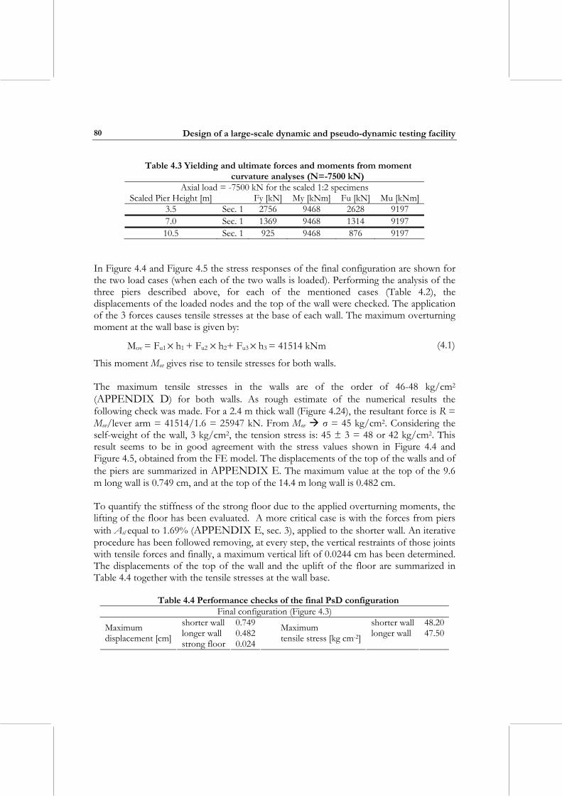
Design of a large-scale dynamic and pseudo-dynamic testing facility
80
Table 4.3 Yielding and ultimate forces and moments from moment curvature analyses (N=-7500 kN)
Axial load = -7500 kN for the scaled 1:2 specimens Scaled Pier Height [m] Fy [kN] My [kNm] Fu [kN] Mu [kNm]
3.5 Sec. 1 2756 9468 2628 9197 7.0 Sec. 1 1369 9468 1314 9197 10.5 Sec. 1 925 9468 876 9197
In Figure 4.4 and Figure 4.5 the stress responses of the final configuration are shown for the two load cases (when each of the two walls is loaded). Performing the analysis of the three piers described above, for each of the mentioned cases (Table 4.2), the displacements of the loaded nodes and the top of the wall were checked. The application of the 3 forces causes tensile stresses at the base of each wall. The maximum overturning moment at the wall base is given by:
Mov = Fu1 × h1 + Fu2 × h2+ Fu3 × h3 = 41514 kNm (4.1)
This moment Mov gives rise to tensile stresses for both walls. The maximum tensile stresses in the walls are of the order of 46-48 kg/cm2 (APPENDIX D) for both walls. As rough estimate of the numerical results the following check was made. For a 2.4 m thick wall (Figure 4.24), the resultant force is R = Mov/lever arm = 41514/1.6 = 25947 kN. From Mov σ = 45 kg/cm2. Considering the self-weight of the wall, 3 kg/cm2, the tension stress is: 45 ± 3 = 48 or 42 kg/cm2. This result seems to be in good agreement with the stress values shown in Figure 4.4 and Figure 4.5, obtained from the FE model. The displacements of the top of the walls and of the piers are summarized in APPENDIX E. The maximum value at the top of the 9.6 m long wall is 0.749 cm, and at the top of the 14.4 m long wall is 0.482 cm. To quantify the stiffness of the strong floor due to the applied overturning moments, the lifting of the floor has been evaluated. A more critical case is with the forces from piers with Asl equal to 1.69% (APPENDIX E, sec. 3), applied to the shorter wall. An iterative procedure has been followed removing, at every step, the vertical restraints of those joints with tensile forces and finally, a maximum vertical lift of 0.0244 cm has been determined. The displacements of the top of the wall and the uplift of the floor are summarized in Table 4.4 together with the tensile stresses at the wall base.
Table 4.4 Performance checks of the final PsD configuration Final configuration (Figure 4.3)
shorter wall 0.749 shorter wall 48.20 longer wall 0.482 longer wall 47.50 Maximum
displacement [cm] strong floor 0.024
Maximum tensile stress [kg cm-2]
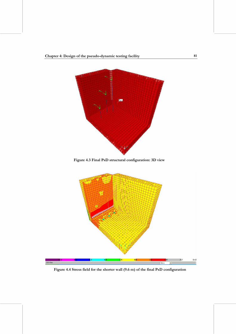
Chapter 4: Design of the pseudo-dynamic testing facility
81
Figure 4.3 Final PsD structural configuration: 3D view
Figure 4.4 Stress field for the shorter wall (9.6 m) of the final PsD configuration
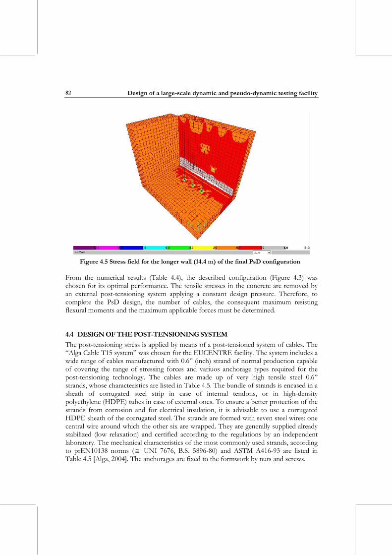
Design of a large-scale dynamic and pseudo-dynamic testing facility
82
Figure 4.5 Stress field for the longer wall (14.4 m) of the final PsD configuration
From the numerical results (Table 4.4), the described configuration (Figure 4.3) was chosen for its optimal performance. The tensile stresses in the concrete are removed by an external post-tensioning system applying a constant design pressure. Therefore, to complete the PsD design, the number of cables, the consequent maximum resisting flexural moments and the maximum applicable forces must be determined.
4.4 DESIGN OF THE POST-TENSIONING SYSTEM The post-tensioning stress is applied by means of a post-tensioned system of cables. The “Alga Cable T15 system” was chosen for the EUCENTRE facility. The system includes a wide range of cables manufactured with 0.6” (inch) strand of normal production capable of covering the range of stressing forces and variuos anchorage types required for the post-tensioning technology. The cables are made up of very high tensile steel 0.6” strands, whose characteristics are listed in Table 4.5. The bundle of strands is encased in a sheath of corrugated steel strip in case of internal tendons, or in high-density polyethylene (HDPE) tubes in case of external ones. To ensure a better protection of the strands from corrosion and for electrical insulation, it is advisable to use a corrugated HDPE sheath of the corrugated steel. The strands are formed with seven steel wires: one central wire around which the other six are wrapped. They are generally supplied already stabilized (low relaxation) and certified according to the regulations by an independent laboratory. The mechanical characteristics of the most commonly used strands, according to prEN10138 norms ( ≅ UNI 7676, B.S. 5896-80) and ASTM A416-93 are listed in Table 4.5 [Alga, 2004]. The anchorages are fixed to the formwork by nuts and screws.
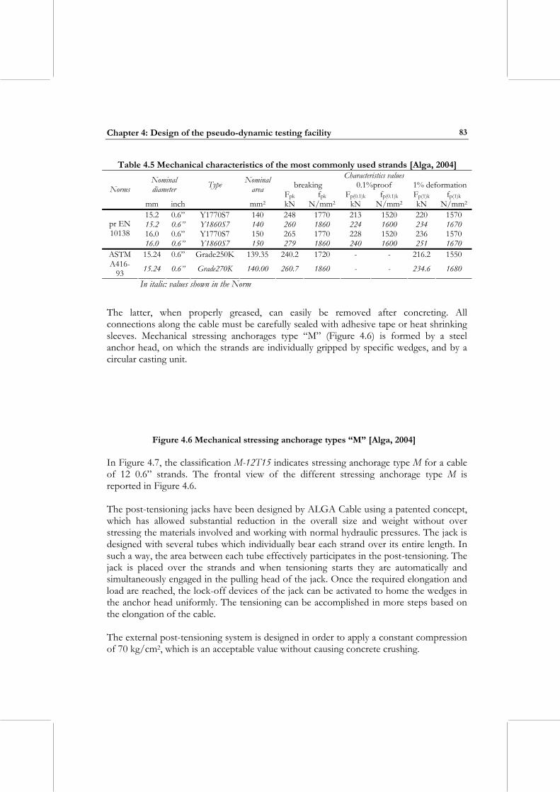
Chapter 4: Design of the pseudo-dynamic testing facility
83
Table 4.5 Mechanical characteristics of the most commonly used strands [Alga, 2004] Characteristics values
breaking 0.1%proof 1% deformationNominal diameter Type Nominal
area Fpk fpk Fp(0.1)k fp(0.1)k Fp(1)k fp(1)k Norms
mm inch mm2 kN N/mm2 kN N/mm2 kN N/mm2
15.2 0.6” Y1770S7 140 248 1770 213 1520 220 1570 15.2 0.6” Y1860S7 140 260 1860 224 1600 234 1670 16.0 0.6” Y1770S7 150 265 1770 228 1520 236 1570
pr EN 10138
16.0 0.6” Y1860S7 150 279 1860 240 1600 251 1670 15.24 0.6” Grade250K 139.35 240.2 1720 - - 216.2 1550 ASTM
A416-93 15.24 0.6” Grade270K 140.00 260.7 1860 - - 234.6 1680
In italic: values shown in the Norm
The latter, when properly greased, can easily be removed after concreting. All connections along the cable must be carefully sealed with adhesive tape or heat shrinking sleeves. Mechanical stressing anchorages type “M” (Figure 4.6) is formed by a steel anchor head, on which the strands are individually gripped by specific wedges, and by a circular casting unit.
Figure 4.6 Mechanical stressing anchorage types “M” [Alga, 2004]
In Figure 4.7, the classification M-12T15 indicates stressing anchorage type M for a cable of 12 0.6” strands. The frontal view of the different stressing anchorage type M is reported in Figure 4.6. The post-tensioning jacks have been designed by ALGA Cable using a patented concept, which has allowed substantial reduction in the overall size and weight without over stressing the materials involved and working with normal hydraulic pressures. The jack is designed with several tubes which individually bear each strand over its entire length. In such a way, the area between each tube effectively participates in the post-tensioning. The jack is placed over the strands and when tensioning starts they are automatically and simultaneously engaged in the pulling head of the jack. Once the required elongation and load are reached, the lock-off devices of the jack can be activated to home the wedges in the anchor head uniformly. The tensioning can be accomplished in more steps based on the elongation of the cable. The external post-tensioning system is designed in order to apply a constant compression of 70 kg/cm2, which is an acceptable value without causing concrete crushing.
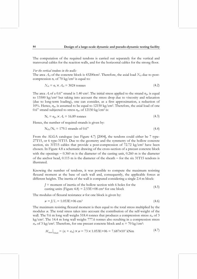
Design of a large-scale dynamic and pseudo-dynamic testing facility
84
The computation of the required tendons is carried out separately for the vertical and transversal cables for the reaction walls, and for the horizontal cables for the strong floor. For the vertical tendons in the walls: The area Acb of the concrete block is 43200cm2. Therefore, the axial load Ncb due to post-compression σc of 70 kg/cm2 is equal to:
Ncb = σc × Acb = 3024 tonnes (4.2)
The area As of a 0.6” strand is 1.40 cm2. The initial stress applied to the strand σpc is equal to 13500 kg/cm2 but taking into account the stress drop due to viscosity and relaxation (due to long-term loading), one can consider, as a first approximation, a reduction of 10%. Hence, σpc is assumed to be equal to 12150 kg/cm2. Therefore, the axial load of one 0.6” strand subjected to stress σpc of 12150 kg/cm2 is:
Ns = σpc × As = 16.89 tonnes (4.3)
Hence, the number of required strands is given by:
Ncb/Ns = 179.1 strands of 0.6” (4.4)
From the ALGA catalogue (see Figure 4.7) [2004], the tendons could either be 7 type-27T15, or 6 type-31T15. Due to the geometry and the symmetry of the hollow concrete section, six 31T15 cables that provide a post-compression of 72.72 kg/cm2 have been chosen. In Figure 4.8 a schematic drawing of the cross-section of a precast concrete block with the openings − 0.360 m is the diameter of the casting unit, 0.260 m is the diameter of the anchor head, 0.115 m is the diameter of the sheath − for the six 31T15 tendons is illustrated. Knowing the number of tendons, it was possible to compute the maximum resisting flexural moment at the base of each wall and, consequently, the applicable forces at different heights. The inertia of the wall is computed considering a single 2.4 m block:
J = moment of inertia of the hollow section with 6 holes for the casting units (Figure 4.8) = 2.53E+08 cm4 for one block (4.5)
The modulus of flexural resistance w for one block is given by:
w = J/L = 1.053E+06 cm3 (4.6)
The maximum resisting flexural moment is then equal to the total stress multiplied by the modulus w. The total stress takes into account the contribution of the self-weight of the wall. The 9.6 m long wall weighs 518.4 tonnes that produces a compression stress σsw of 3 kg/cm2. The 14.4 m long wall weighs 777.6 tonnes also resulting in a compression stress σsw of 3 kg/cm2. Therefore, for one precast concrete block and σc = 70 kg/cm2:
blockM 1max = (σc + σsw) × w = 73 × 1.053E+06 = 7.687×10⁷ kNm (4.7)
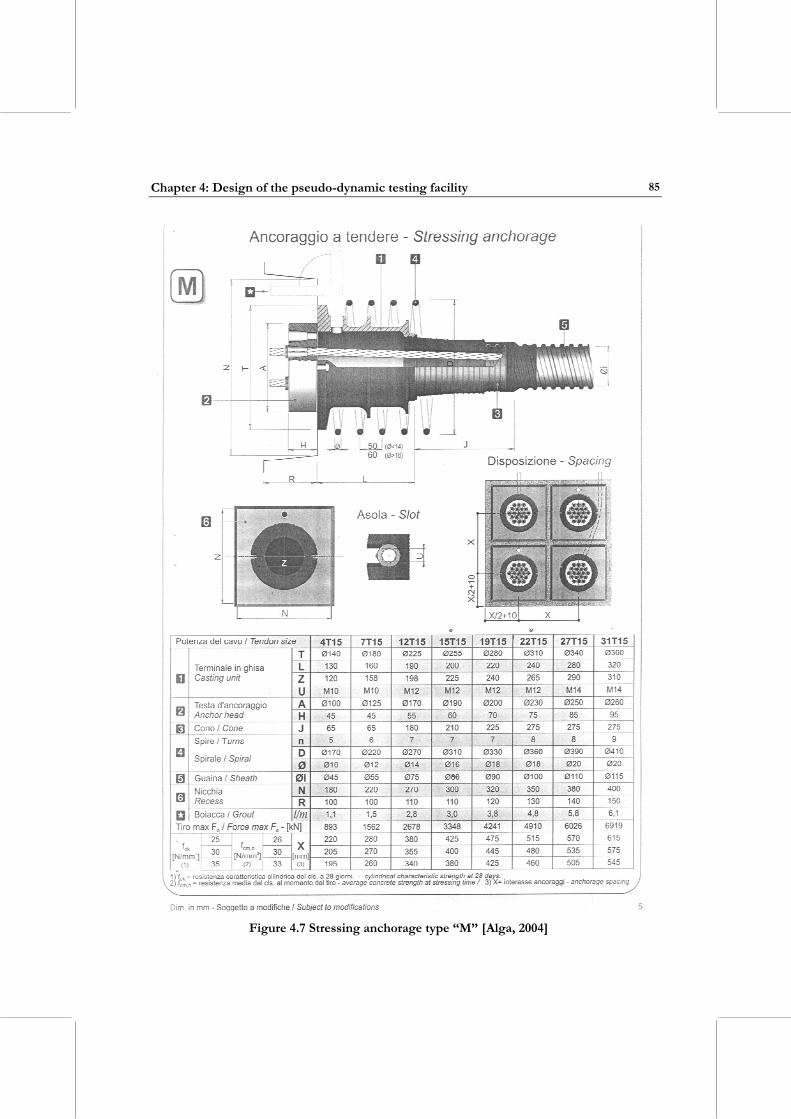
Chapter 4: Design of the pseudo-dynamic testing facility
85
Figure 4.7 Stressing anchorage type “M” [Alga, 2004]
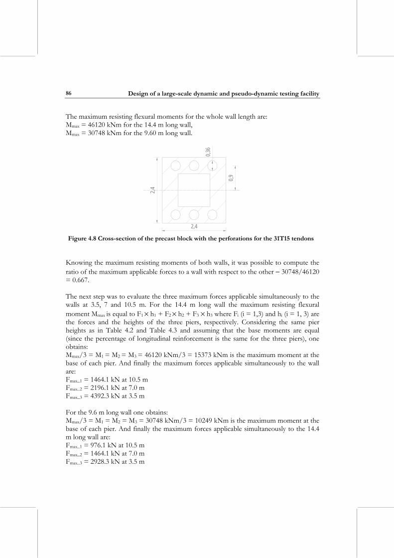
Design of a large-scale dynamic and pseudo-dynamic testing facility
86
The maximum resisting flexural moments for the whole wall length are: Mmax = 46120 kNm for the 14.4 m long wall, Mmax = 30748 kNm for the 9.60 m long wall.
0,9
2,4
2,4
0,36
Figure 4.8 Cross-section of the precast block with the perforations for the 31T15 tendons
Knowing the maximum resisting moments of both walls, it was possible to compute the ratio of the maximum applicable forces to a wall with respect to the other − 30748/46120 = 0.667. The next step was to evaluate the three maximum forces applicable simultaneously to the walls at 3.5, 7 and 10.5 m. For the 14.4 m long wall the maximum resisting flexural moment Mmax is equal to F1 × h1 + F2 × h2 + F3 × h3 where Fi (i = 1,3) and hi (i = 1, 3) are the forces and the heights of the three piers, respectively. Considering the same pier heights as in Table 4.2 and Table 4.3 and assuming that the base moments are equal (since the percentage of longitudinal reinforcement is the same for the three piers), one obtains: Mmax/3 = M1 = M2 = M3 = 46120 kNm/3 = 15373 kNm is the maximum moment at the base of each pier. And finally the maximum forces applicable simultaneously to the wall are: Fmax_1 = 1464.1 kN at 10.5 m Fmax_2 = 2196.1 kN at 7.0 m Fmax_3 = 4392.3 kN at 3.5 m For the 9.6 m long wall one obtains: Mmax/3 = M1 = M2 = M3 = 30748 kNm/3 = 10249 kNm is the maximum moment at the base of each pier. And finally the maximum forces applicable simultaneously to the 14.4 m long wall are: Fmax_1 = 976.1 kN at 10.5 m Fmax_2 = 1464.1 kN at 7.0 m Fmax_3 = 2928.3 kN at 3.5 m
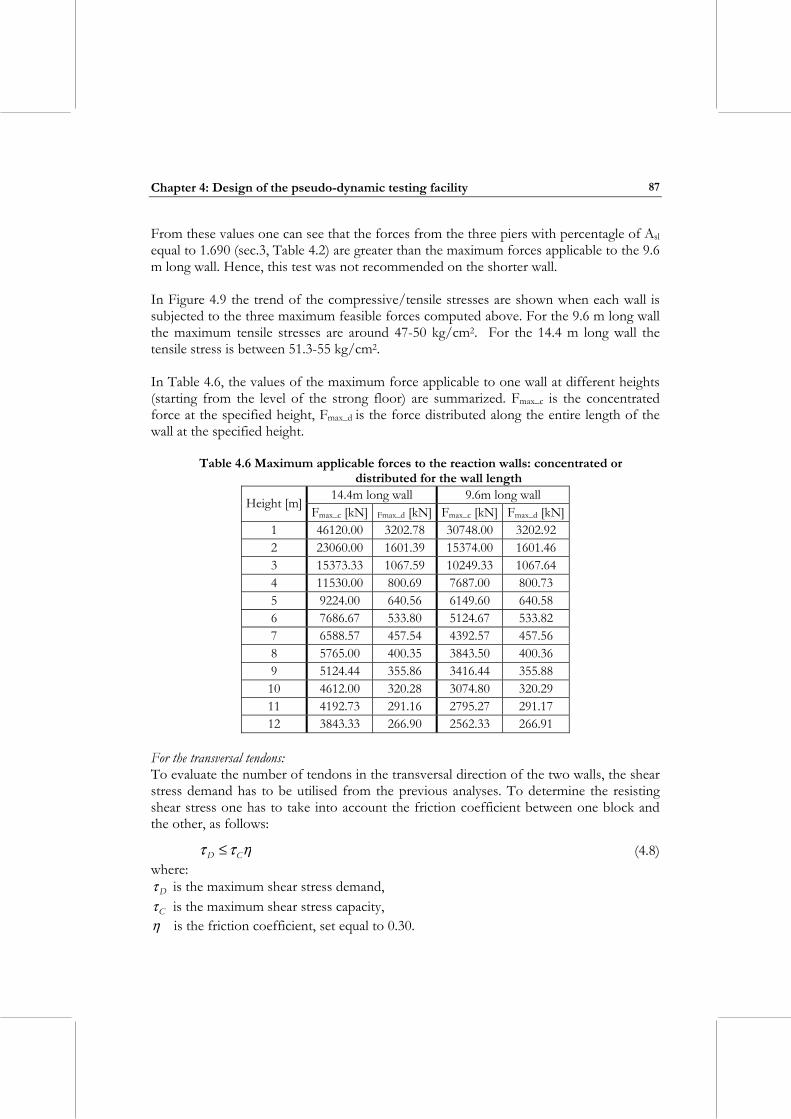
Chapter 4: Design of the pseudo-dynamic testing facility
87
From these values one can see that the forces from the three piers with percentagle of Asl equal to 1.690 (sec.3, Table 4.2) are greater than the maximum forces applicable to the 9.6 m long wall. Hence, this test was not recommended on the shorter wall. In Figure 4.9 the trend of the compressive/tensile stresses are shown when each wall is subjected to the three maximum feasible forces computed above. For the 9.6 m long wall the maximum tensile stresses are around 47-50 kg/cm2. For the 14.4 m long wall the tensile stress is between 51.3-55 kg/cm2. In Table 4.6, the values of the maximum force applicable to one wall at different heights (starting from the level of the strong floor) are summarized. Fmax_c is the concentrated force at the specified height, Fmax_d is the force distributed along the entire length of the wall at the specified height.
Table 4.6 Maximum applicable forces to the reaction walls: concentrated or distributed for the wall length
14.4m long wall 9.6m long wall Height [m] Fmax_c [kN] Fmax_d [kN] Fmax_c [kN] Fmax_d [kN]
1 46120.00 3202.78 30748.00 3202.92 2 23060.00 1601.39 15374.00 1601.46 3 15373.33 1067.59 10249.33 1067.64 4 11530.00 800.69 7687.00 800.73 5 9224.00 640.56 6149.60 640.58 6 7686.67 533.80 5124.67 533.82 7 6588.57 457.54 4392.57 457.56 8 5765.00 400.35 3843.50 400.36 9 5124.44 355.86 3416.44 355.88 10 4612.00 320.28 3074.80 320.29 11 4192.73 291.16 2795.27 291.17 12 3843.33 266.90 2562.33 266.91
For the transversal tendons: To evaluate the number of tendons in the transversal direction of the two walls, the shear stress demand has to be utilised from the previous analyses. To determine the resisting shear stress one has to take into account the friction coefficient between one block and the other, as follows:
ηττ CD ≤ (4.8)where:
Dτ is the maximum shear stress demand, Cτ is the maximum shear stress capacity,
η is the friction coefficient, set equal to 0.30.
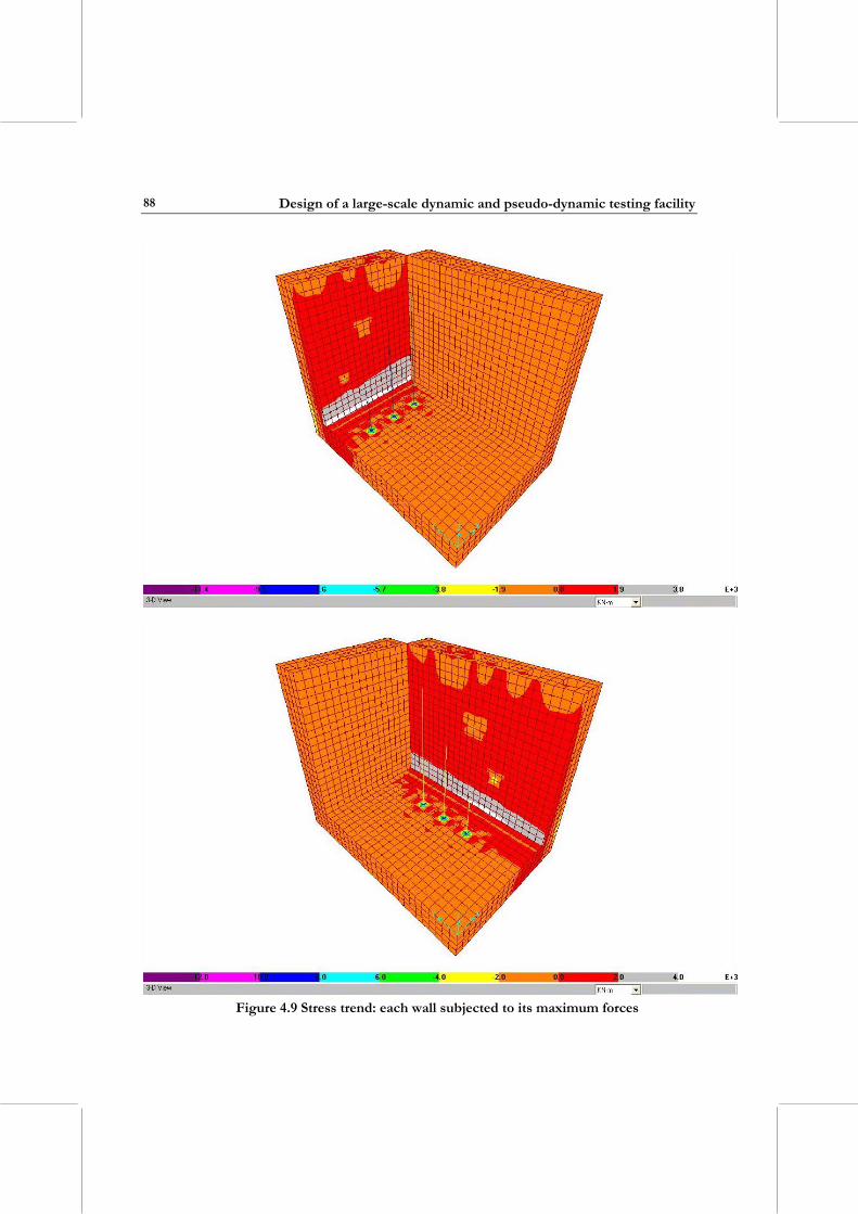
Design of a large-scale dynamic and pseudo-dynamic testing facility
88
Figure 4.9 Stress trend: each wall subjected to its maximum forces
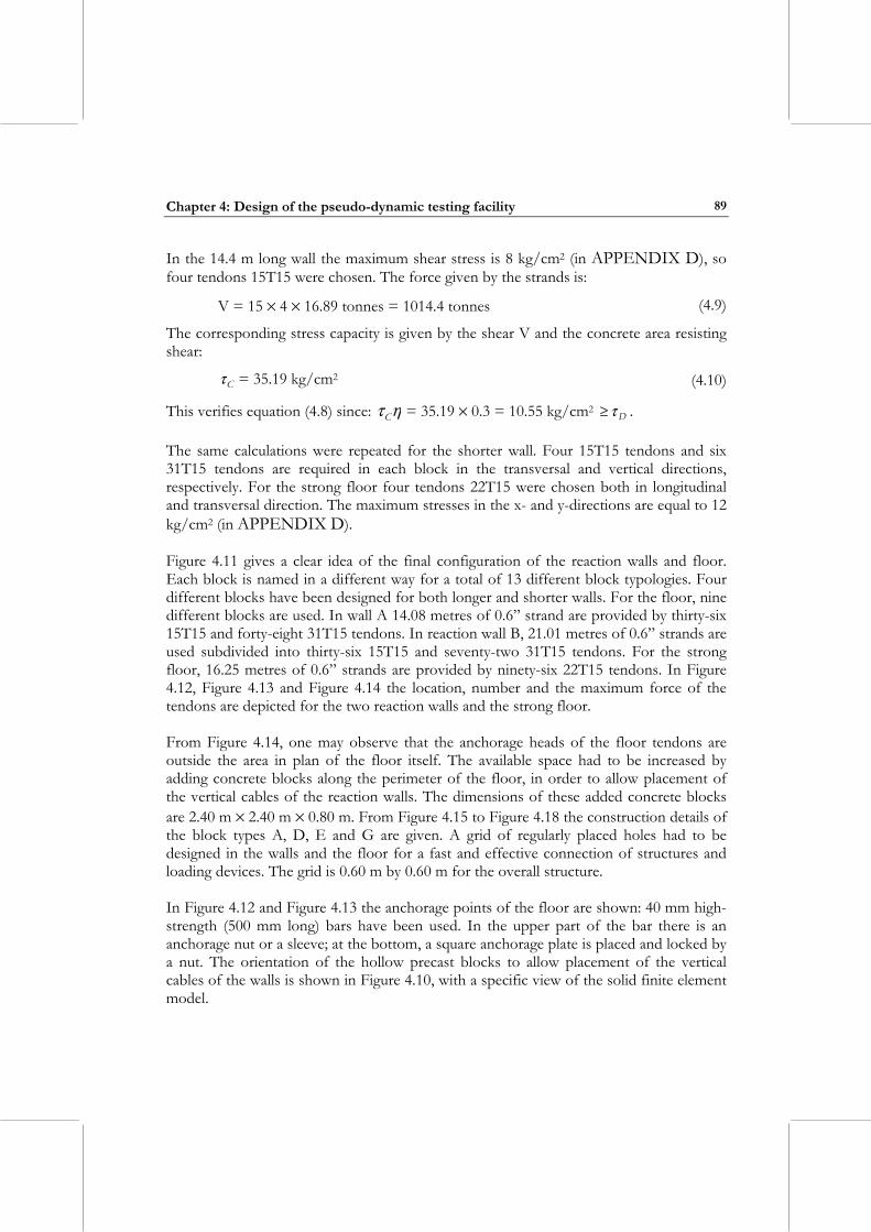
Chapter 4: Design of the pseudo-dynamic testing facility
89
In the 14.4 m long wall the maximum shear stress is 8 kg/cm2 (in APPENDIX D), so four tendons 15T15 were chosen. The force given by the strands is:
V = 15 × 4 × 16.89 tonnes = 1014.4 tonnes (4.9)
The corresponding stress capacity is given by the shear V and the concrete area resisting shear:
Cτ = 35.19 kg/cm2 (4.10)
This verifies equation (4.8) since: ητC = 35.19 × 0.3 = 10.55 kg/cm2 Dτ≥ . The same calculations were repeated for the shorter wall. Four 15T15 tendons and six 31T15 tendons are required in each block in the transversal and vertical directions, respectively. For the strong floor four tendons 22T15 were chosen both in longitudinal and transversal direction. The maximum stresses in the x- and y-directions are equal to 12 kg/cm2 (in APPENDIX D). Figure 4.11 gives a clear idea of the final configuration of the reaction walls and floor. Each block is named in a different way for a total of 13 different block typologies. Four different blocks have been designed for both longer and shorter walls. For the floor, nine different blocks are used. In wall A 14.08 metres of 0.6” strand are provided by thirty-six 15T15 and forty-eight 31T15 tendons. In reaction wall B, 21.01 metres of 0.6” strands are used subdivided into thirty-six 15T15 and seventy-two 31T15 tendons. For the strong floor, 16.25 metres of 0.6” strands are provided by ninety-six 22T15 tendons. In Figure 4.12, Figure 4.13 and Figure 4.14 the location, number and the maximum force of the tendons are depicted for the two reaction walls and the strong floor. From Figure 4.14, one may observe that the anchorage heads of the floor tendons are outside the area in plan of the floor itself. The available space had to be increased by adding concrete blocks along the perimeter of the floor, in order to allow placement of the vertical cables of the reaction walls. The dimensions of these added concrete blocks are 2.40 m × 2.40 m × 0.80 m. From Figure 4.15 to Figure 4.18 the construction details of the block types A, D, E and G are given. A grid of regularly placed holes had to be designed in the walls and the floor for a fast and effective connection of structures and loading devices. The grid is 0.60 m by 0.60 m for the overall structure. In Figure 4.12 and Figure 4.13 the anchorage points of the floor are shown: 40 mm high-strength (500 mm long) bars have been used. In the upper part of the bar there is an anchorage nut or a sleeve; at the bottom, a square anchorage plate is placed and locked by a nut. The orientation of the hollow precast blocks to allow placement of the vertical cables of the walls is shown in Figure 4.10, with a specific view of the solid finite element model.
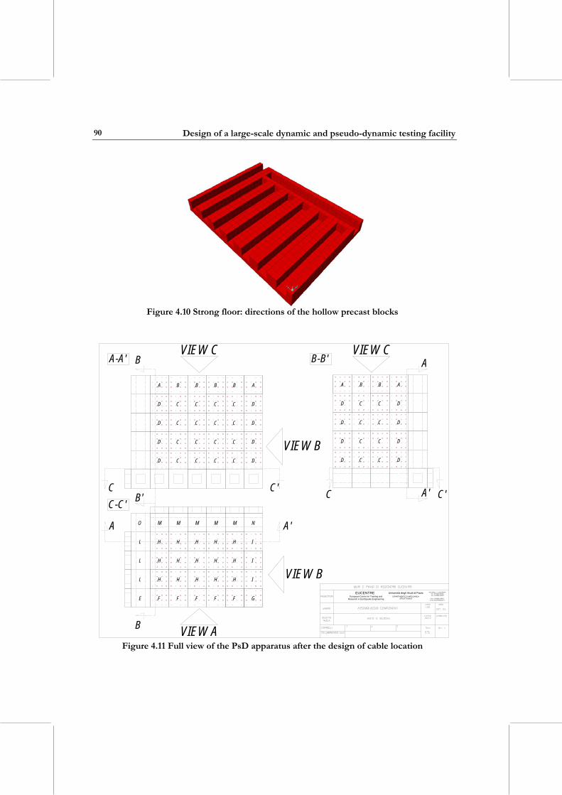
Design of a large-scale dynamic and pseudo-dynamic testing facility
90
Figure 4.10 Strong floor: directions of the hollow precast blocks
A B B B B A
D C C C C D
D C C C C D
D C C C C D
D C C C C D
F F F F F G
I
I
IH
H
H
H
H
H
H
H
H
H
H
H
H
H
H
D
D
D
C
C
C
C
B
C
C
C
C
B
D
D
A
D
D
A
D
E
L
L
L
M NM M M MO
VIEW B
VIEW A
VIEW B
VIEW C VIEW C
A'A
B
B'C C'
A-A' B-B'
C-C'
DIPARTIMENTO DI MECCANICA STRUTTURALE
Università degli Studi di PaviaEuropean Centre for Training and
Research in Earthquake Engineering
EUCENTRE Via Ferrata, 1 - 27100 PAVIATel. +39 0382 505468Tel. +39 0382 505451
Fax. +39 0382 528422E-mail [email protected]
B
C'C
A
A'
Figure 4.11 Full view of the PsD apparatus after the design of cable location
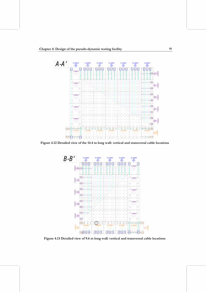
Chapter 4: Design of the pseudo-dynamic testing facility
91
11.440kN
24.180kN
7.800kN
7.800kN
11.440kN 11.440kN
7.800kN
7.800kN
3.900kN
24.180kN 24.180kN 24.180kN
11.440kN 11.440kN 11.440kN
24.180kN 24.180kN 24.180kN
11.440kN
A-A'
Figure 4.12 Detailed view of the 14.4 m long wall: vertical and transversal cable locations
B-B'3.900kN
7.800kN
7.800kN
7.800kN
7.800kN
11.440kN 11.440kN 11.440kN 11.440kN 11.440kN
Figure 4.13 Detailed view of 9.6 m long wall: vertical and transversal cable locations
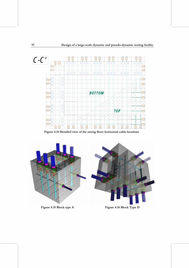
Design of a large-scale dynamic and pseudo-dynamic testing facility
92
BOTTOM
TOP
C-C'
Figure 4.14 Detailed view of the strong floor: horizontal cable locations
Figure 4.15 Block type A Figure 4.16 Block Type D
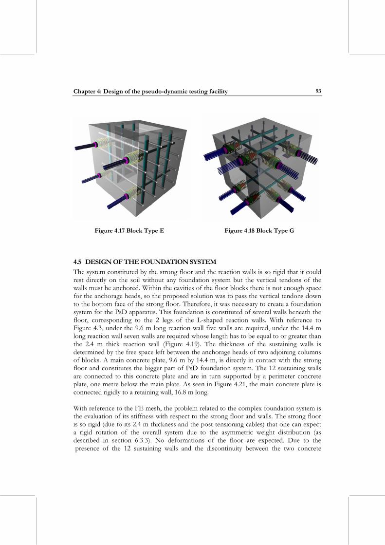
Chapter 4: Design of the pseudo-dynamic testing facility
93
Figure 4.17 Block Type E Figure 4.18 Block Type G
4.5 DESIGN OF THE FOUNDATION SYSTEM The system constituted by the strong floor and the reaction walls is so rigid that it could rest directly on the soil without any foundation system but the vertical tendons of the walls must be anchored. Within the cavities of the floor blocks there is not enough space for the anchorage heads, so the proposed solution was to pass the vertical tendons down to the bottom face of the strong floor. Therefore, it was necessary to create a foundation system for the PsD apparatus. This foundation is constituted of several walls beneath the floor, corresponding to the 2 legs of the L-shaped reaction walls. With reference to Figure 4.3, under the 9.6 m long reaction wall five walls are required, under the 14.4 m long reaction wall seven walls are required whose length has to be equal to or greater than the 2.4 m thick reaction wall (Figure 4.19). The thickness of the sustaining walls is determined by the free space left between the anchorage heads of two adjoining columns of blocks. A main concrete plate, 9.6 m by 14.4 m, is directly in contact with the strong floor and constitutes the bigger part of PsD foundation system. The 12 sustaining walls are connected to this concrete plate and are in turn supported by a perimeter concrete plate, one metre below the main plate. As seen in Figure 4.21, the main concrete plate is connected rigidly to a retaining wall, 16.8 m long. With reference to the FE mesh, the problem related to the complex foundation system is the evaluation of its stiffness with respect to the strong floor and walls. The strong floor is so rigid (due to its 2.4 m thickness and the post-tensioning cables) that one can expect a rigid rotation of the overall system due to the asymmetric weight distribution (as described in section 6.3.3). No deformations of the floor are expected. Due to the presence of the 12 sustaining walls and the discontinuity between the two concrete
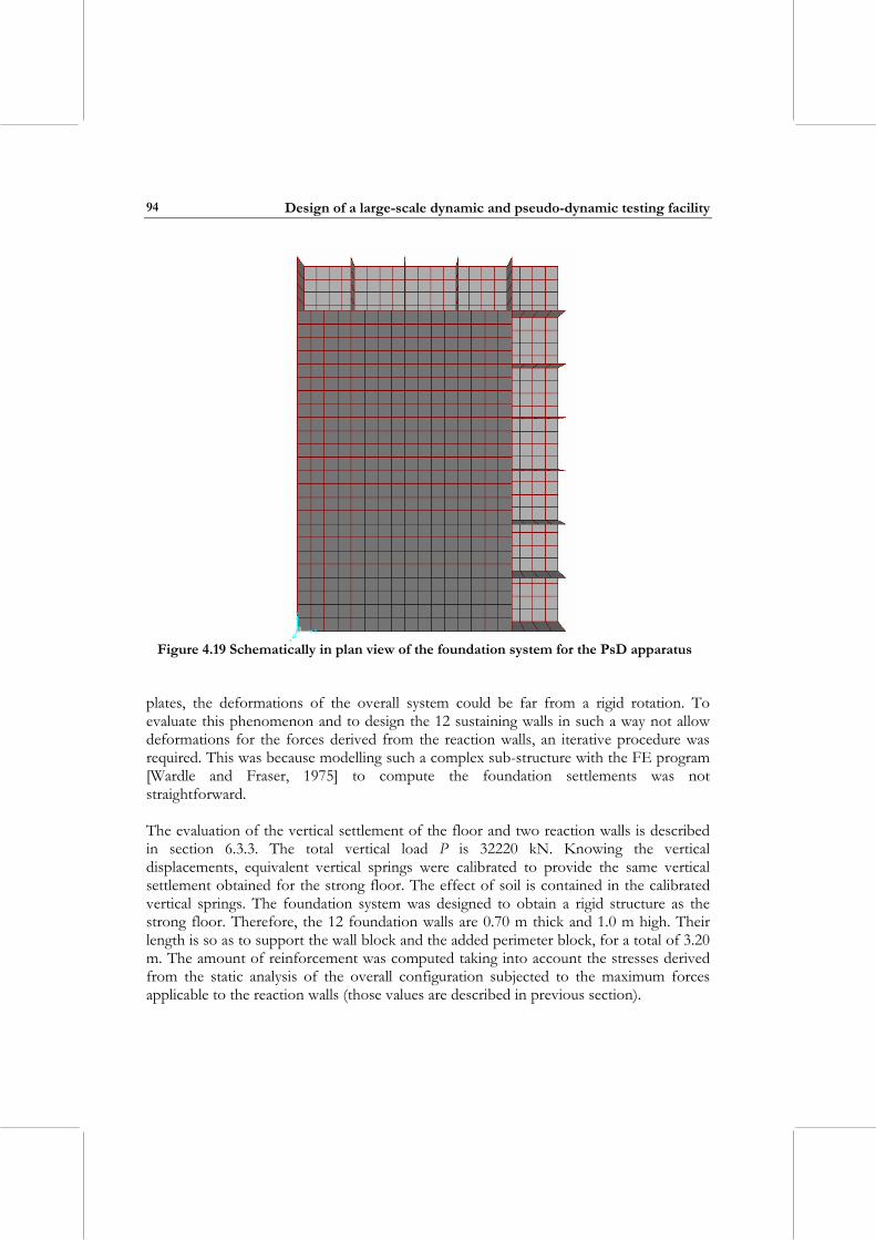
Design of a large-scale dynamic and pseudo-dynamic testing facility
94
Figure 4.19 Schematically in plan view of the foundation system for the PsD apparatus
plates, the deformations of the overall system could be far from a rigid rotation. To evaluate this phenomenon and to design the 12 sustaining walls in such a way not allow deformations for the forces derived from the reaction walls, an iterative procedure was required. This was because modelling such a complex sub-structure with the FE program [Wardle and Fraser, 1975] to compute the foundation settlements was not straightforward. The evaluation of the vertical settlement of the floor and two reaction walls is described in section 6.3.3. The total vertical load P is 32220 kN. Knowing the vertical displacements, equivalent vertical springs were calibrated to provide the same vertical settlement obtained for the strong floor. The effect of soil is contained in the calibrated vertical springs. The foundation system was designed to obtain a rigid structure as the strong floor. Therefore, the 12 foundation walls are 0.70 m thick and 1.0 m high. Their length is so as to support the wall block and the added perimeter block, for a total of 3.20 m. The amount of reinforcement was computed taking into account the stresses derived from the static analysis of the overall configuration subjected to the maximum forces applicable to the reaction walls (those values are described in previous section).
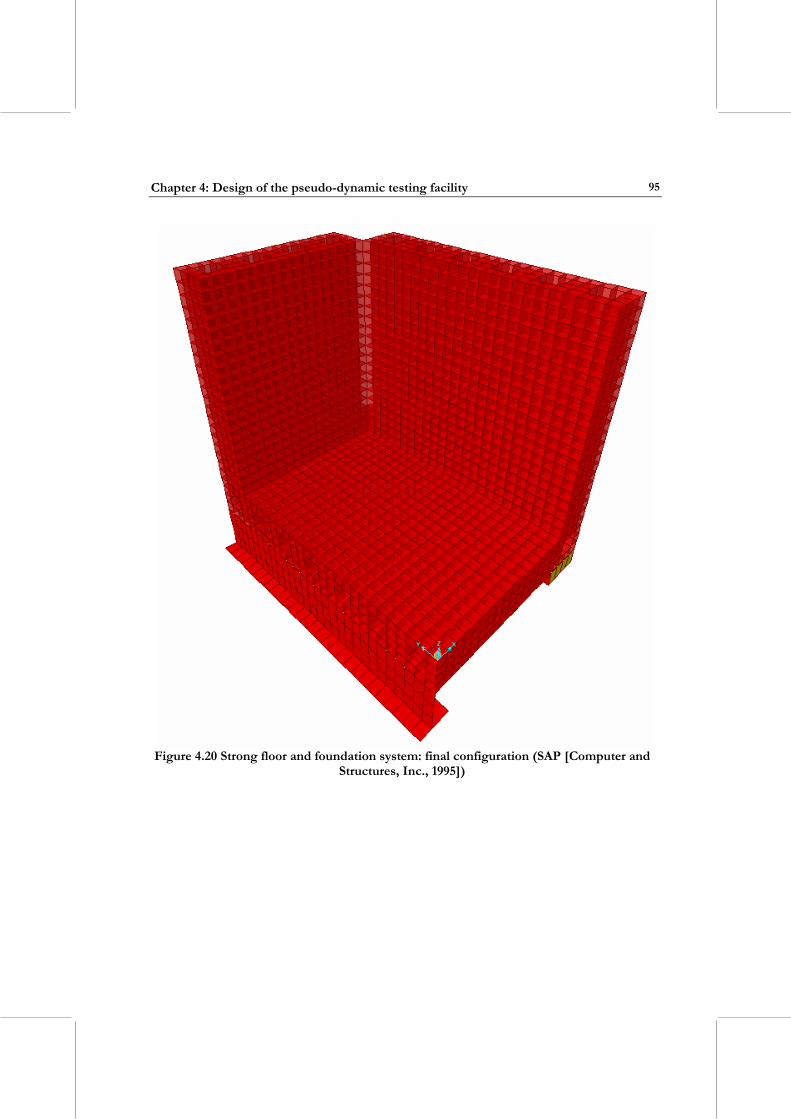
Chapter 4: Design of the pseudo-dynamic testing facility
95
Figure 4.20 Strong floor and foundation system: final configuration (SAP [Computer and
Structures, Inc., 1995])
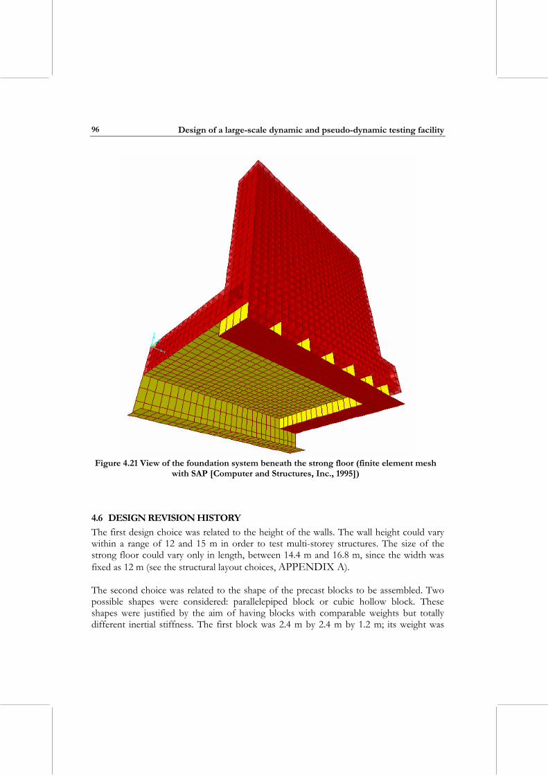
Design of a large-scale dynamic and pseudo-dynamic testing facility
96
Figure 4.21 View of the foundation system beneath the strong floor (finite element mesh
with SAP [Computer and Structures, Inc., 1995])
4.6 DESIGN REVISION HISTORY The first design choice was related to the height of the walls. The wall height could vary within a range of 12 and 15 m in order to test multi-storey structures. The size of the strong floor could vary only in length, between 14.4 m and 16.8 m, since the width was fixed as 12 m (see the structural layout choices, APPENDIX A). The second choice was related to the shape of the precast blocks to be assembled. Two possible shapes were considered: parallelepiped block or cubic hollow block. These shapes were justified by the aim of having blocks with comparable weights but totally different inertial stiffness. The first block was 2.4 m by 2.4 m by 1.2 m; its weight was
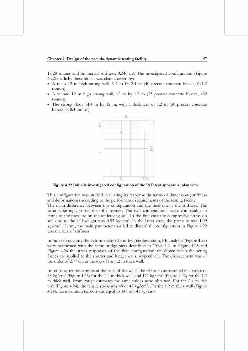
Chapter 4: Design of the pseudo-dynamic testing facility
97
17.28 tonnes and its inertial stiffness, 0.346 m4. The investigated configuration (Figure 4.22) made by these blocks was characterized by: • A main 12 m high strong wall, 9.6 m by 2.4 m (40 precast concrete blocks, 691.2
tonnes), • A second 12 m high strong wall, 12 m by 1.2 m (25 precast concrete blocks, 432
tonnes), • The strong floor 14.4 m by 12 m, with a thickness of 1.2 m (30 precast concrete
blocks, 518.4 tonnes).
9,6
9,6
12
122,4
14,4
1,21,2
Figure 4.22 Initially investigated configuration of the PsD test apparatus: plan view
This configuration was studied evaluating its response (in terms of dimensions, stiffness and deformations) according to the performance requirements of the testing facility. The main difference between this configuration and the final one is the stiffness. The latter is strongly stiffer than the former. The two configurations were comparable in terms of the pressure on the underlying soil. In the first case the compressive stress on soil due to the self-weight was 0.95 kg/cm2; in the latter case, the pressure was 1.09 kg/cm2. Hence, the main parameter that led to discard the configuration in Figure 4.22 was the lack of stiffness. In order to quantify the deformability of this first configuration, FE analyses (Figure 4.23) were performed with the same bridge piers described in Table 4.2. In Figure 4.25 and Figure 4.26 the stress responses of the first configuration are shown when the acting forces are applied to the shorter and longer walls, respectively. The displacement was of the order of 2.77 cm at the top of the 1.2 m thick wall. In terms of tensile stresses at the base of the walls, the FE analyses resulted in a stress of 48 kg/cm2 (Figure 4.25) for the 2.4 m thick wall, and 171 kg/cm2 (Figure 4.26) for the 1.2 m thick wall. From rough estimates the same values were obtained. For the 2.4 m tick wall (Figure 4.24), the tensile stress was 48 or 42 kg/cm2. For the 1.2 m thick wall (Figure 4.24), the maximum tension was equal to 147 or 141 kg/cm2.
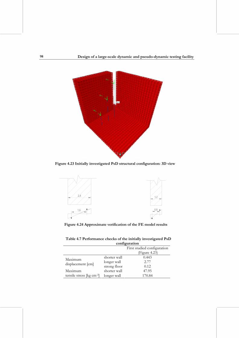
Design of a large-scale dynamic and pseudo-dynamic testing facility
98
Figure 4.23 Initially investigated PsD structural configuration: 3D view
2,4
1,6
0,8
1,2
Figure 4.24 Approximate verification of the FE model results
Table 4.7 Performance checks of the initially investigated PsD
configuration First studied configuration
(Figure 4.23) shorter wall 0.443 longer wall 2.77 Maximum
displacement [cm] strong floor 0.12 shorter wall 47.95 Maximum
tensile stress [kg cm-2] longer wall 170.84
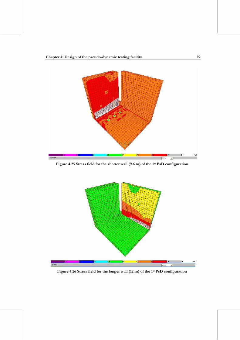
Chapter 4: Design of the pseudo-dynamic testing facility
99
Figure 4.25 Stress field for the shorter wall (9.6 m) of the 1st PsD configuration
Figure 4.26 Stress field for the longer wall (12 m) of the 1st PsD configuration

Design of a large-scale dynamic and pseudo-dynamic testing facility
100
From the numerical results (Table 4.7), it can be observed that the first configuration was not appropriate since the 12 m long wall was too flexible (its top displacement was almost 3 cm) and the tensile stress was unacceptable. There was no post-tensioning system able to absorb this large stress without causing crushing of the concrete. And, finally, the uplift of the floor was not negligible.
CHAPTER 5: ACTUATOR SYSTEM
In the following sections some details of the design solution for the EUCENTRE testing facility are reported. The information presented in the sections 5.2 and 5.3 is with reference to that supplied by MTS System Corporation [2004]. A brief description of the piping system for the pressurized oil distribution is given. The information has been supplied by Hydros s.r.l [2004].
5.1 APPLICATIONS OF EXTERNAL ACTIONS During the set-up of an experimental investigation, engineers must make several decisions related to the application of external actions. The first decision will stem from the choice of test being performed; be it pseudo-static, pseudo-dynamic, or a fully dynamic test. In the case of the pseudo-static and pseudo-dynamic tests, the engineer needs to select an appropriate type of jack or hydraulic actuator. If a fully dynamic seismic investigation into the non-linear range is to be performed, then application of external actions is currently limited to the use of shaking tables. Non-destructive dynamic testing can be computed using ambient or small-amplitude forced vibrations. There are important considerations to be given to the application of external actions, as described in Sullivan et al. [2004]. Forces and displacements can be applied to a structure using one of the following devices:
a) Screw jacks, b) Flat jacks, c) Hydraulic jacks, d) Hydraulic actuators.
Consideration should be given to the range of displacements and forces that must be applied and these should be checked against the limits of the jacks and actuators available. a) Screw jacks Screw jacks incorporate a threaded shaft or gearing system that allows extension or retraction of a bearing plate at the end of the jack. They are designed for both tensile and compressive loads and will operate in any orientation or mounting position. They can be flexibly configured, either be installed singly, in pairs, or as part of a multiple jack system. The jacks can control both forces and displacements manually or by an electric, hydraulic or pneumatic motor, however, an external transducer is required in order to apply rotations. Further positive characteristics of screw jacks are that they have a wide range of
Design of a large-scale dynamic and pseudo-dynamic testing facility
102
load capabilities, and variations in speed are available, according to the screw type and gearing. However, as the jacks cannot apply loads and displacements at high velocity they are currently limited to use in static types of tests. Manufacturers provide a wide range of screw jacks with special features such as anti-rotation designs, anti backlash options and other safety features. b) Flat jacks Flat-jacks are typically circular low flat units which are capable of exerting high-pressure forces. They are used by the construction industry for a multitude of applications, such as lifting heavy structures, transferring existing loads to temporary or permanent supports and permanently preloading replacement bridge bearings. Due to their design, they are only light in weight but require a minimal installation gap of just a few centimeters. In typical seismic testing situations, flat-jacks are installed only temporarily. Flat-jacks intended for temporary installation can be inflated using hydraulic or resin pumping equipment. The flat-jacks should be inserted leaving ample clearance to allow for shimming tight prior to inflation. Extraction devices can be attached to flat jacks with steel plates to allow ease of removal upon completion of jacking. It is apparent that the flat-jacks only allow application of pressure forces and therefore are suitable principally for quasi-static testing without cycling. A typical application of flat jacks is in the assessment of the compressive stresses in masonry walls. c) Hydraulic jacks Hydraulic jacks consist of a piston within which it is possible to inject or withdraw viscous fluid at pressure. The pressure pushes the oil against the piston plate moving an arm which is attached to the structure being acted upon. The hydraulic jacks can be configured so that both tensile and compressive forces can be applied to a structure. The force applied to the structure is simply the product of the oil pressure and the piston area. Neglecting the compressibility of oil, the flow rate within the jack is given by the velocity of the piston multiplied again by the section area of the piston and consequently it is evident that the maximum flow rate of the hydraulic system limits the velocity of the piston. To ensure long life of hydraulic jacks, installation of a high performance oil filter unit within the hydraulic system is worthwhile as is the performance of regular maintenance of the bearings and gaskets. To enable application of forces in both tensile and compression, hydraulic jacks have been developed with the ability to inject oil from both sides of the piston plate. The main limitation associated with the use of hydraulic jacks in seismic engineering is that they do not allow quick control of the applied force, and consequently they are best suited to static tests. d) Hydraulic actuators The forces are applied through hydraulic actuators which, differently from other testing devices like hydraulic jacks, are able to quickly control the applied forces. This control is achieved with servovalve that can inject oil and change the pressure within the cylinder of the actuator very quickly. Actuators typically allow application of motions with frequency
Chapter 5: Actuator system
103
from 0 to 150 or 200 Hz. Because of the quick control and relatively high forces that can be provided by hydraulic actuators, they are a very useful tool for dynamic seismic testing. To ensure long life of hydraulic actuators, installation of a high performance oil filter unit within the hydraulic system is worthwhile as is the performance of regular maintenance. The actuators in shaking tables are generally quite long and thin because of the requirements for long stroke and high velocity. This means that the actuators have some axial flexibility and will have the potential for bending laterally like pin-ended struts. The natural frequency of the axial mode of a normally proportioned actuator is generally high (>100 Hz) while the natural frequency of the bending mode is likely to be lower (generally 2 or 3 times higher than the natural frequency of the oil column). These frequencies are relatively high in relation to the operating frequency of the table and hence are, in general, unlikely to be particularly significant. Of all the possible resonances that can be introduced into a shaking table, the most important is probably the oil column resonance [Clark, 1992]. This is because it is likely to have a low frequency, often well within the operating range of the shaking table, and is unlikely to be highly damped. The natural frequency of the oil column in any actuator can be calculated from:
LmKAf ⋅=
π21 (5.1)
where: f = natural frequency of the oil column (Hz), K = bulk modulus of the hydraulic oil (N/m2), A = effective cross sectional area of the oil column in the actuator (m2), L = length of the oil column (m), m = effective mass of the platform and specimen being excited by the actuator (kg). The effect of this temperature dependence can be seen in the table below where the changing bulk modulus causes the natural frequency of an oil column to change by 12% over a range of 30°C. This change in natural frequency of the system may be of particular importance if, during a test the oil temperature rises and the natural frequency of the oil column drops closer to a natural frequency of the specimen being tested. Not only do the dynamic characteristics of the table change but also the possibility of table-specimen interaction becomes more likely. It should be noted that the bulk modulus of the oil is temperature dependant and this should be taken into account when calculating the natural frequency of the oil column.
Design of a large-scale dynamic and pseudo-dynamic testing facility
104
Table 5.1 Dependency of oil column resonance on oil temperature [Crewe, 1998]
Oil temperature [°C] Bulk modulus [N/m2] Natural frequency10 2.272 × 10⁹ 18.720 20 2.110 × 10⁹ 18.025 30 1.947 × 10⁹ 17.326 40 1.785 × 10⁹ 16.590 100 1.315 × 10⁹ 14.239
To perform dynamic and pseudo-dynamic tests hydraulic actuators are used. Hydraulic actuators have been designed by the manufacturers, MTS System Corporation, to meet the performance requirements of a powerful dynamic and pseudo-dynamic facility at the EUCENTRE laboratory. The MTS System Corporation designed a special and unique piece as the hydraulic actuator of the shaking table whereas for the PsD apparatus, standard devices have been chosen.
5.2 ACTUATOR SYSTEM OF THE SHAKING TABLE For the EUCENTRE shaking table, the longitudinal hydraulic actuator is provided by MTS System Corporation, Eden Prairie, Minnesota. The high-performance actuator (type 244) has a dynamic capacity of ± 1700 kN (at 280 bar supply pressure) and a static capacity of ± 2116 kN. The total dynamic stroke is equal to 1000 mm ( ± 500 mm); the total static stroke is 1152.4 mm. The fatigue-rated actuator assembly includes the following: • Hollow single-piece rod. • Dual (qty-2) Model 256.80 three-stage sleeve type servovalve rated at 3000 l/min (70
bar pressure drop. Higher flows at corresponding higher pressures). Each valve has 252.43 type pilot valve.
• Linear variable displacement transducer (LVDT): type stroke transducer. • Close-coupled pressure and return accumulators, 200 litres for pressure, and 100 litres
for return. • Differential pressure cells • Hydraulic cushions sized for 85 tonnes mass (table+specimen) • Low-friction hydrostatic rod bearings • Refer to performance curve for actuator performance data (Figure 5.1):
Based on the specifications of the servo-hydraulic components described as follows, the performance curves of the EUCENTRE shaking table in a tripartite plot are shown in Figure 5.1. Table performance envelopes for a bare table condition and a table loaded with a 60 tonnes (Mton in the plot) payload are provided. These performance curves were generated based on the final design platform weight of 32.90 tonnes. Figure 5.1 also shows that the maximum acceleration input of the EUCENTRE shaking table is a function of the vertical payload on the table. For a bare table the performance curve indicates an acceleration in excess of 5.0g, which tends to reduce with the increase of
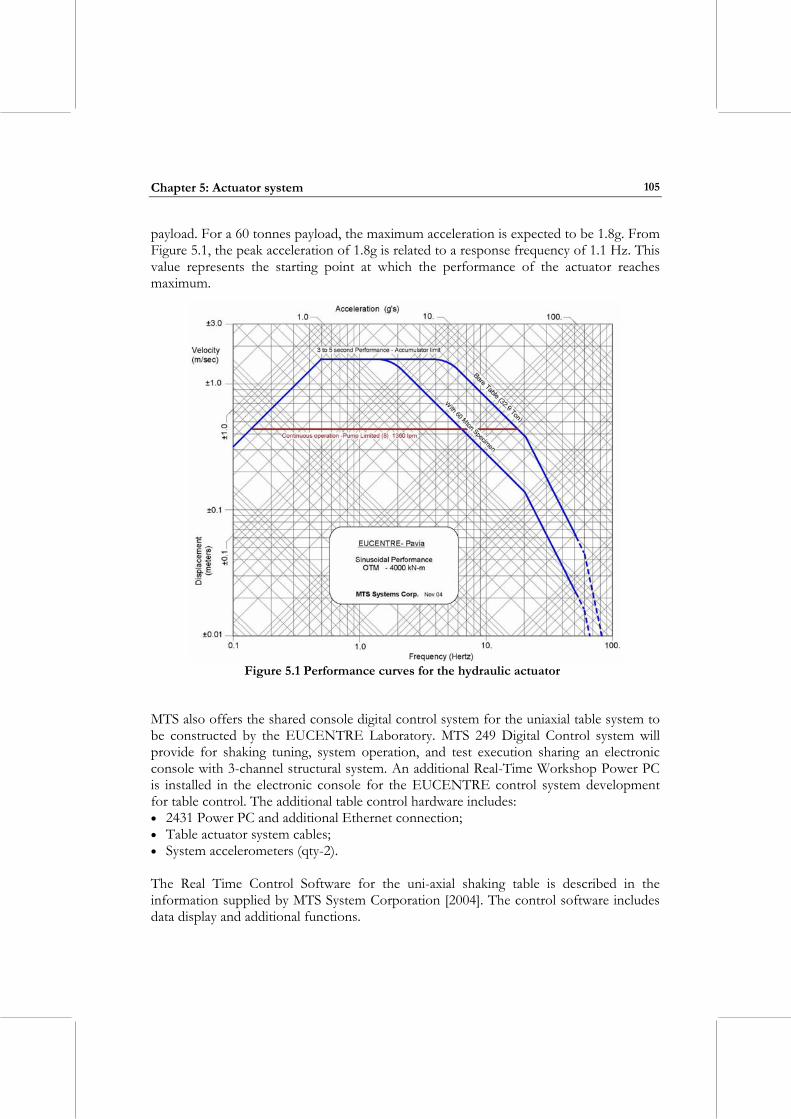
Chapter 5: Actuator system
105
payload. For a 60 tonnes payload, the maximum acceleration is expected to be 1.8g. From Figure 5.1, the peak acceleration of 1.8g is related to a response frequency of 1.1 Hz. This value represents the starting point at which the performance of the actuator reaches maximum.
Figure 5.1 Performance curves for the hydraulic actuator
MTS also offers the shared console digital control system for the uniaxial table system to be constructed by the EUCENTRE Laboratory. MTS 249 Digital Control system will provide for shaking tuning, system operation, and test execution sharing an electronic console with 3-channel structural system. An additional Real-Time Workshop Power PC is installed in the electronic console for the EUCENTRE control system development for table control. The additional table control hardware includes: • 2431 Power PC and additional Ethernet connection; • Table actuator system cables; • System accelerometers (qty-2). The Real Time Control Software for the uni-axial shaking table is described in the information supplied by MTS System Corporation [2004]. The control software includes data display and additional functions.
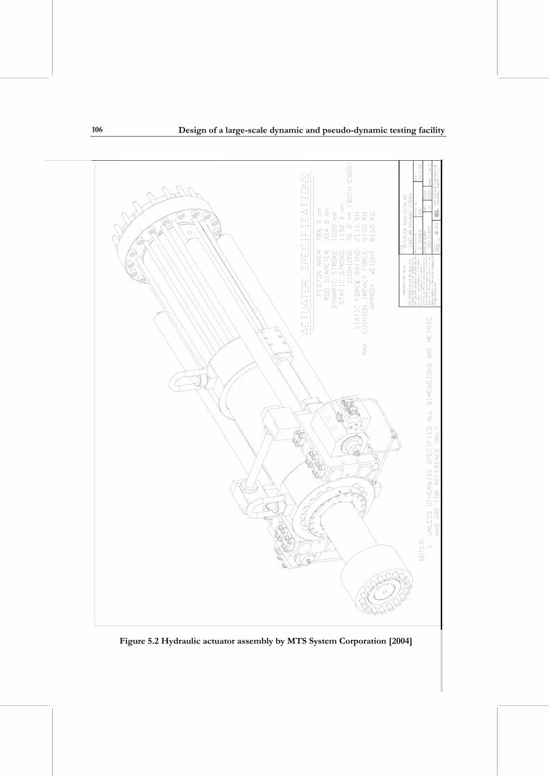
Design of a large-scale dynamic and pseudo-dynamic testing facility
106
Figure 5.2 Hydraulic actuator assembly by MTS System Corporation [2004]
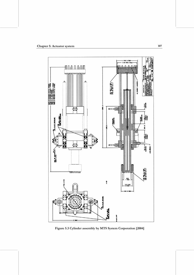
Chapter 5: Actuator system
107
Figure 5.3 Cylinder assembly by MTS System Corporation [2004]
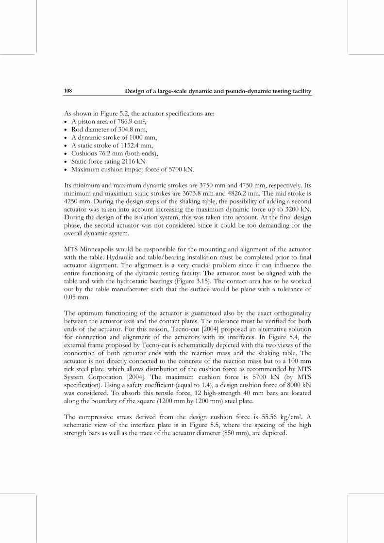
Design of a large-scale dynamic and pseudo-dynamic testing facility
108
As shown in Figure 5.2, the actuator specifications are: • A piston area of 786.9 cm2, • Rod diameter of 304.8 mm, • A dynamic stroke of 1000 mm, • A static stroke of 1152.4 mm, • Cushions 76.2 mm (both ends), • Static force rating 2116 kN • Maximum cushion impact force of 5700 kN. Its minimum and maximum dynamic strokes are 3750 mm and 4750 mm, respectively. Its minimum and maximum static strokes are 3673.8 mm and 4826.2 mm. The mid stroke is 4250 mm. During the design steps of the shaking table, the possibility of adding a second actuator was taken into account increasing the maximum dynamic force up to 3200 kN. During the design of the isolation system, this was taken into account. At the final design phase, the second actuator was not considered since it could be too demanding for the overall dynamic system. MTS Minneapolis would be responsible for the mounting and alignment of the actuator with the table. Hydraulic and table/bearing installation must be completed prior to final actuator alignment. The alignment is a very crucial problem since it can influence the entire functioning of the dynamic testing facility. The actuator must be aligned with the table and with the hydrostatic bearings (Figure 3.15). The contact area has to be worked out by the table manufacturer such that the surface would be plane with a tolerance of 0.05 mm. The optimum functioning of the actuator is guaranteed also by the exact orthogonality between the actuator axis and the contact plates. The tolerance must be verified for both ends of the actuator. For this reason, Tecno-cut [2004] proposed an alternative solution for connection and alignment of the actuators with its interfaces. In Figure 5.4, the external frame proposed by Tecno-cut is schematically depicted with the two views of the connection of both actuator ends with the reaction mass and the shaking table. The actuator is not directly connected to the concrete of the reaction mass but to a 100 mm tick steel plate, which allows distribution of the cushion force as recommended by MTS System Corporation [2004]. The maximum cushion force is 5700 kN (by MTS specification). Using a safety coefficient (equal to 1.4), a design cushion force of 8000 kN was considered. To absorb this tensile force, 12 high-strength 40 mm bars are located along the boundary of the square (1200 mm by 1200 mm) steel plate. The compressive stress derived from the design cushion force is 55.56 kg/cm2. A schematic view of the interface plate is in Figure 5.5, where the spacing of the high strength bars as well as the trace of the actuator diameter (850 mm), are depicted.
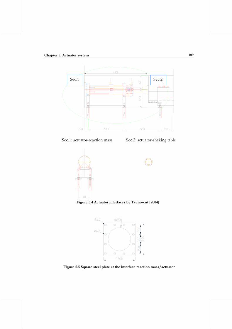
Chapter 5: Actuator system
109
Sec.1: actuator-reaction mass Sec.2: actuator-shaking table
Sec.1 Sec.2
Figure 5.4 Actuator interfaces by Tecno-cut [2004]
Figure 5.5 Square steel plate at the interface reaction mass/actuator
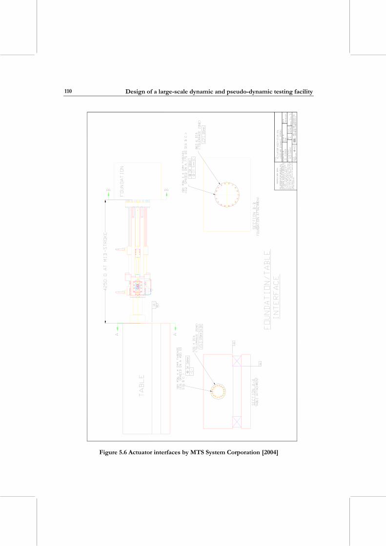
Design of a large-scale dynamic and pseudo-dynamic testing facility
110
Figure 5.6 Actuator interfaces by MTS System Corporation [2004]
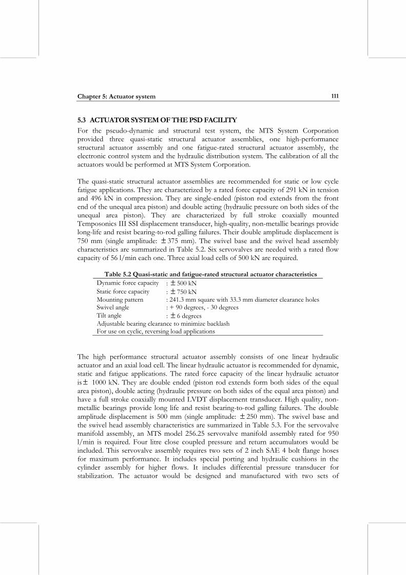
Chapter 5: Actuator system
111
5.3 ACTUATOR SYSTEM OF THE PSD FACILITY For the pseudo-dynamic and structural test system, the MTS System Corporation provided three quasi-static structural actuator assemblies, one high-performance structural actuator assembly and one fatigue-rated structural actuator assembly, the electronic control system and the hydraulic distribution system. The calibration of all the actuators would be performed at MTS System Corporation. The quasi-static structural actuator assemblies are recommended for static or low cycle fatigue applications. They are characterized by a rated force capacity of 291 kN in tension and 496 kN in compression. They are single-ended (piston rod extends from the front end of the unequal area piston) and double acting (hydraulic pressure on both sides of the unequal area piston). They are characterized by full stroke coaxially mounted Temposonics III SSI displacement transducer, high-quality, non-metallic bearings provide long-life and resist bearing-to-rod galling failures. Their double amplitude displacement is 750 mm (single amplitude: ± 375 mm). The swivel base and the swivel head assembly characteristics are summarized in Table 5.2. Six servovalves are needed with a rated flow capacity of 56 l/min each one. Three axial load cells of 500 kN are required.
Table 5.2 Quasi-static and fatigue-rated structural actuator characteristics Dynamic force capacity : ± 500 kN Static force capacity : ± 750 kN Mounting pattern : 241.3 mm square with 33.3 mm diameter clearance holes Swivel angle : + 90 degrees, - 30 degrees Tilt angle : ± 6 degrees Adjustable bearing clearance to minimize backlash For use on cyclic, reversing load applications
The high performance structural actuator assembly consists of one linear hydraulic actuator and an axial load cell. The linear hydraulic actuator is recommended for dynamic, static and fatigue applications. The rated force capacity of the linear hydraulic actuator is ± 1000 kN. They are double ended (piston rod extends form both sides of the equal area piston), double acting (hydraulic pressure on both sides of the equal area piston) and have a full stroke coaxially mounted LVDT displacement transducer. High quality, non-metallic bearings provide long life and resist bearing-to-rod galling failures. The double amplitude displacement is 500 mm (single amplitude: ± 250 mm). The swivel base and the swivel head assembly characteristics are summarized in Table 5.3. For the servovalve manifold assembly, an MTS model 256.25 servovalve manifold assembly rated for 950 l/min is required. Four litre close coupled pressure and return accumulators would be included. This servovalve assembly requires two sets of 2 inch SAE 4 bolt flange hoses for maximum performance. It includes special porting and hydraulic cushions in the cylinder assembly for higher flows. It includes differential pressure transducer for stabilization. The actuator would be designed and manufactured with two sets of
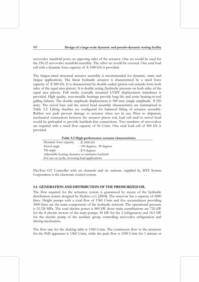
Design of a large-scale dynamic and pseudo-dynamic testing facility
112
servovalve manifold ports on opposing sides of the actuator. One set would be used for the 256.25 servovalve manifold assembly. The other set would be covered. One axial load cell with a dynamic force capacity of ± 1000 kN is provided. The fatigue-rated structural actuator assembly is recommended for dynamic, static and fatigue applications. The linear hydraulic actuator is characterized by a rated force capacity of ± 500 kN. It is characterized by double ended (piston rod extends form both sides of the equal area piston). It is double acting (hydraulic pressure on both sides of the equal area piston). Full stroke coaxially mounted LVDT displacement transducer is provided. High quality, non-metallic bearings provide long life and resist bearing-to-rod galling failures. The double amplitude displacement is 500 mm (single amplitude: ± 250 mm). The swivel base and the swivel head assembly characteristics are summarized in Table 5.2. Lifting shackles are configured for balanced lifting of actuator assembly. Rubber rest pads prevent damage to actuator when not in use. Prior to shipment, mechanical connections between the actuator piston rod, load cell and/or swivel head would be preloaded to provide backlash-free connections. Two numbers of servovalves are required with a rated flow capacity of 56 l/min. One axial load cell of 500 kN is provided.
Table 5.3 High-performance actuator characteristics Dynamic force capacity : ± 1000 kN Swivel angle : +90 degrees, -30 degrees Tilt angle : ± 8 degrees Adjustable bearing clearance to minimize backlash For use on cyclic, reversing load applications
FlexTest GT Controller with six channels and six stations, supplied by MTS System Corporation is the electronic control system.
5.4 GENERATION AND DISTRIBUTION OF THE PRESSURIZED OIL The flow required for the actuation system is guaranteed by means of the hydraulic distribution system designed by Hydros s.r.l. [2004]. The reservoir has a capacity of 6000 litres. Height pumps with a total flow of 1360 l/min and five accumulators providing 3000 litres are the main components of the hydraulic network. The operational pressure is 21/28 MPa. The total electric power is 800 kW those main contributions are 720 kW for the 8 electric motors of the main pumps, 50 kW for the 2 refrigerators and 18.5 kW for the electric pump of the auxiliary group controlling servovalve refrigeration and driving mechanism. The flow rate for the shaking table is 1360 l/min. The continuous flow to the actuators for the PsD apparatus is 1360 l/min, while the peak flow is 1500 l/min for 1 minute or
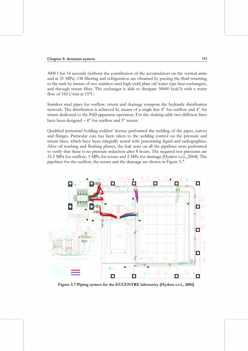
Chapter 5: Actuator system
113
3000 l for 14 seconds (without the contribution of the accumulators on the vertical arms and at 21 MPa). Oil filtering and refrigeration are obtained by passing the fluid returning to the tank by means of two stainless steel high-yield plate oil/water type heat exchangers, and through return filter. The exchanger is able to dissipate 50000 kcal/h with a water flow of 160 l/min at 15°C. Stainless steel pipes for outflow, return and drainage compose the hydraulic distribution network. The distribution is achieved by means of a single line 4” for outflow and 4” for return dedicated to the PsD apparatus operation. For the shaking table two different lines have been designed − 4” for outflow and 5” return. Qualified personnel holding welders’ license performed the welding of the pipes, curves and flanges. Particular care has been taken to the welding control on the pressure and return lines, which have been integrally tested with penetrating liquid and radiographies. After oil washing and flushing phases, the leak tests on all the pipelines were performed to verify that there is no pressure reduction after 8 hours. The required test pressures are 31.5 MPa for outflow, 3 MPa for return and 2 MPa for drainage [Hydros s.r.l., 2004]. The pipelines for the outflow, the return and the drainage are shown in Figure 5.7.
Figure 5.7 Piping system for the EUCENTRE laboratory [Hydros s.r.l., 2004]

CHAPTER 6: SOIL-STRUCTURE INTERACTION
This chapter is devoted to the soil-structure interaction problem. The definition of the dynamic properties of the foundation soil is given. The evaluation of the static vertical settlement of both the shaking table and the PsD apparatus is presented. A description of the dynamic soil-foundation structure interaction due to the excitations of the shaking table then follows.
6.1 ASPECTS OF SOIL-STRUCTURE INTERACTION INVESTIGATIONS A good design of a testing facility has to consider all the aspects and phenomena related to the interaction of the facility with the soil. Hence, it is important to know exactly the present conditions of the soil, its material composition, layering, trend of its mechanical parameters like the shear wave velocity and the Poisson’s ratio (Section 6.2). The initial computation consists of the evaluation of the vertical settlement due to the static load condition. The evaluation of vertical displacements is important since it can influence the behaviour of the overall facility. If differential displacements can exist, the stationary condition of the facility is influenced. The presence of asymmetric configurations causes these differential displacements. For the shaking table (section 6.3.2), the reaction mass-table-specimen system constitutes a non-equilibrated structure due to the eccentric position of the table (with respect to the reaction mass centre of gravity), and of the specimen (due to its own configuration). The vertical loads can be transmitted either directly to the foundation system (if the reaction mass rests directly on the foundation) or through the isolation system at the foundation. In the first case, the stiffness of the reaction mass should be large enough to cause a rigid rotation of the foundation, which, in turn, has to be a rigid structure. In the second case, the isolation system does not allow a uniform load distribution: there are as many lumped loads as the number of isolators. Obviously the isolation system has to be designed to balance the effect of the unbalanced mass distribution and of the overturning moment (even if the latter has its influence only in the dynamic field). It is clear that the presence of possible differential displacements causes significant problems for the stability and the operation of the shaking table, the actuation system, and the hydrostatic bearings whose required accuracy is high. For the pseudo-dynamic facility (section 6.3.3) the presence of differential displacements has to be taken into account for a correct working of the facility. The advantage of the
Design of a large-scale dynamic and pseudo-dynamic testing facility
116
PsD apparatus with respect to the shaking table is that the strong walls and floor represent a very stiff system whose weight is transmitted to the foundation/soil through a thick floor. The load distribution in the PsD apparatus is not balanced due to asymmetric positioning of the reaction walls with respect to the strong floor. Due to the stiffness of the strong floor, the asymmetric configuration could cause a rigid rotation of the basement. The amount of those displacements must be quantified in long and short-term situations. And the foundation system must be stiff enough not to deform as a consequence of the transmitted forces, if it exists. After the evaluation of response under the dead loads and the self-weight of the facility, a more refined study of the dynamic soil-structure interaction problem must be performed to predict the ground motion induced by the excitation of the shaking table (section 6.4.2). Further, it is important to estimate the liquefaction susceptibility of the soil as a function of the acceleration transmitted through the foundation. If the liquefaction potential exists, solutions to improve the soil behaviour are required to prevent the collapse of the entire testing facility. Also the possibility of settlement of saturated sands must be taken into account and quantified as a function of the transmitted acceleration. An accurate study of the dynamic interaction between shaking table and underlying soil has been performed. The amplification of accelerations and displacements transmitted to the reaction mass/foundation/soil corresponding to the isolator resonance frequency led to discarding the airbags. No base isolation has been designed to mitigate the vibration impact induced by the experimental simulations. The results of the study performed to optimize the reaction mass/foundation design are described in section 6.4.1, derived from Pavese et al. [2005].
6.2 DEFINITION OF DYNAMIC PROPERTIES OF FOUNDATION SOIL In the area of study, the following geotechnical investigation campaign was performed: • Two boreholes (BH01 and BH02) until 25 m depth. A standard penetration test (SPT)
every 1.5 m was performed in one borehole. In the second borehole a open wall piezometre was used to determine the water table level;
• One seismic cross-hole test (CH1) until 25 m depth. This test was carried out to determine the profiles of shear wave velocity, Vs, and dilatational wave velocity, Vp, with depth.
The results of the SPT test are depicted in Figure 6.1. The segmented line represents a precautionary estimate of the blow/foot NSPT with the depth. The values of the SPT test show a variation of 10 blow/foot until 14 m in depth. Beyond this there is an increase of NSPT until 37 blow/foot at 20 m in depth. During boring, several specimens have been taken for laboratory tests, like granulometric tests, classification tests, measurements of the volume weight and of the amount of natural water. On the undisturbed samples, taken within the cohesive material layers, endometric and triaxial tests were carried out.
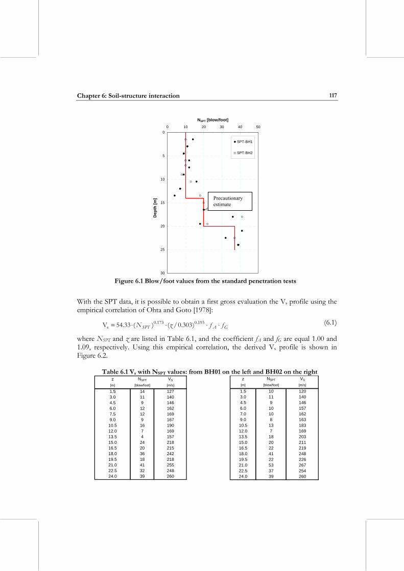
Chapter 6: Soil-structure interaction
117
0
5
10
15
20
25
30
0 10 20 30 40 50
NSPT [blow/foot]
Dep
th [m
]
SPT-BH1
SPT-BH2
cautelative estimate
Precautionary estimate
Figure 6.1 Blow/foot values from the standard penetration tests
With the SPT data, it is possible to obtain a first gross evaluation the Vs profile using the empirical correlation of Ohta and Goto [1978]:
GASPT ffzN ⋅⋅⋅⋅= 193.0173.0s )303.0/()(33.54V (6.1)
where NSPT and z are listed in Table 6.1, and the coefficient fA and fG are equal 1.00 and 1.09, respectively. Using this empirical correlation, the derived Vs profile is shown in Figure 6.2.
Table 6.1 Vs with NSPT values: from BH01 on the left and BH02 on the right z NSPT VS
[m] [blow/foot] [m/s]
1.5 14 1273.0 11 1404.5 9 1466.0 12 1627.5 12 1699.0 9 167
10.5 16 19012.0 7 16913.5 4 15715.0 24 21816.5 20 21518.0 36 24219.5 18 21821.0 41 25522.5 32 24824.0 39 260
z NSPT VS
[m] [blow/foot] [m/s]
1.5 10 1203.0 11 1404.5 9 1466.0 10 1577.0 10 1629.0 8 163
10.5 13 18312.0 7 16913.5 18 20315.0 20 21116.5 22 21918.0 41 24819.5 22 22621.0 53 26722.5 37 25424.0 39 260
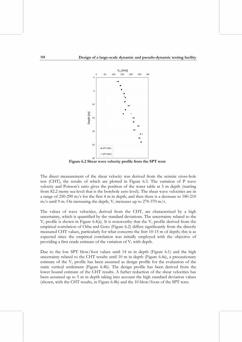
Design of a large-scale dynamic and pseudo-dynamic testing facility
118
0
5
10
15
20
25
30
0 50 100 150 200 250 300
VS [m/s]
Dep
th [m
]
SPT-BH1
SPT-BH2
Figure 6.2 Shear wave velocity profile from the SPT tests
The direct measurement of the shear velocity was derived from the seismic cross-hole test (CHT), the results of which are plotted in Figure 6.3. The variation of P wave velocity and Poisson’s ratio gives the position of the water table at 5 m depth (starting from 82.2 metre sea-level that is the borehole zero level). The shear wave velocities are in a range of 250-290 m/s for the first 4 m in depth, and then there is a decrease to 180-210 m/s until 9 m. On increasing the depth, Vs increases up to 270-370 m/s. The values of wave velocities, derived from the CHT, are characterized by a high uncertainty, which is quantified by the standard deviations. The uncertainty related to the Vs profile is shown in Figure 6.4(a). It is noteworthy that the Vs profile derived from the empirical correlation of Otha and Goto (Figure 6.2) differs significantly from the directly measured CHT values, particularly for what concerns the fisrt 10-15 m of depth; this is as expected since the empirical correlation was initially employed with the objective of providing a first crude estimate of the variation of Vs with depth. Due to the low SPT blow/foot values until 14 m in depth (Figure 6.1) and the high uncertainty related to the CHT results until 10 m in depth (Figure 6.4a), a precautionary estimate of the Vs profile has been assumed as design profile for the evaluation of the static vertical settlement (Figure 6.4b). The design profile has been derived from the lower bound estimate of the CHT results. A furher reduction of the shear velocities has been assumed up to 5 m in depth taking into account the high standard deviation values (shown, with the CHT results, in Figure 6.4b) and the 10 blow/foots of the SPT tests.
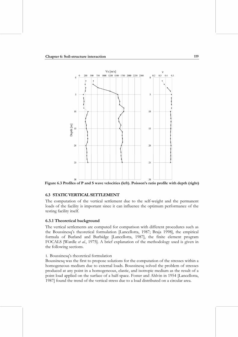
Chapter 6: Soil-structure interaction
119
ν Vs [m/s] D
epth
[m]
Figure 6.3 Profiles of P and S wave velocities (left). Poisson’s ratio profile with depth (right)
6.3 STATIC VERTICAL SETTLEMENT The computation of the vertical settlement due to the self-weight and the permanent loads of the facility is important since it can influence the optimum performance of the testing facility itself.
6.3.1 Theoretical background The vertical settlements are computed for comparison with different procedures such as the Boussinesq’s theoretical formulation [Lancellotta, 1987; Braja 1998], the empirical formula of Burland and Burbidge [Lancellotta, 1987], the finite element program FOCALS [Wardle et al., 1975]. A brief explanation of the methodology used is given in the following sections. 1. Boussinesq’s theoretical formulation Boussinesq was the first to propose solutions for the computation of the stresses within a homogeneous medium due to external loads. Boussinesq solved the problem of stresses produced at any point in a homogeneous, elastic, and isotropic medium as the result of a point load applied on the surface of a half-space. Foster and Ahlvin in 1954 [Lancellotta, 1987] found the trend of the vertical stress due to a load distributed on a circular area.
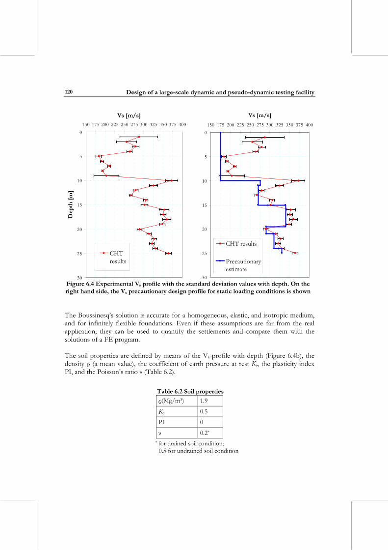
Design of a large-scale dynamic and pseudo-dynamic testing facility
120
0
5
10
15
20
25
30
150 175 200 225 250 275 300 325 350 375 400
Vs [m/s]
Dep
th [m
]
CHTresults
0
5
10
15
20
25
30
150 175 200 225 250 275 300 325 350 375 400
Vs [m/s]
CHT results
Precautionaryestimate
Figure 6.4 Experimental Vs profile with the standard deviation values with depth. On the right hand side, the Vs precautionary design profile for static loading conditions is shown The Boussinesq’s solution is accurate for a homogeneous, elastic, and isotropic medium, and for infinitely flexible foundations. Even if these assumptions are far from the real application, they can be used to quantify the settlements and compare them with the solutions of a FE program. The soil properties are defined by means of the Vs profile with depth (Figure 6.4b), the density ρ (a mean value), the coefficient of earth pressure at rest Ko, the plasticity index PI, and the Poisson’s ratio ν (Table 6.2).
Table 6.2 Soil properties ρ(Mg/m3) 1.9
Ko 0.5
PI 0
ν 0.2* * for drained soil condition; 0.5 for undrained soil condition
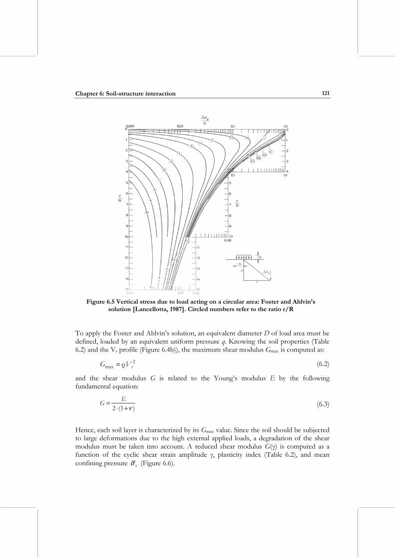
Chapter 6: Soil-structure interaction
121
NUMBERS IN REFER TO THE RATIO r/R
Figure 6.5 Vertical stress due to load acting on a circular area: Foster and Ahlvin’s
solution [Lancellotta, 1987]. Circled numbers refer to the ratio r/R
To apply the Foster and Ahlvin’s solution, an equivalent diameter D of load area must be defined, loaded by an equivalent uniform pressure q. Knowing the soil properties (Table 6.2) and the Vs profile (Figure 6.4b)), the maximum shear modulus Gmax is computed as:
2max ρ sVG = (6.2)
and the shear modulus G is related to the Young’s modulus E by the following fundamental equation:
)1(2 ν+⋅= EG (6.3)
Hence, each soil layer is characterized by its Gmax value. Since the soil should be subjected to large deformations due to the high external applied loads, a degradation of the shear modulus must be taken into account. A reduced shear modulus G(γ) is computed as a function of the cyclic shear strain amplitude γ, plasticity index (Table 6.2), and mean confining pressure oσ (Figure 6.6).
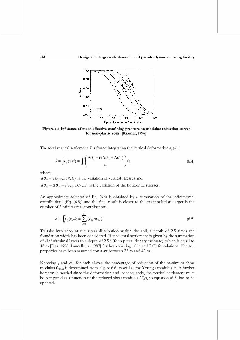
Design of a large-scale dynamic and pseudo-dynamic testing facility
122
Figure 6.6 Influence of mean effective confining pressure on modulus reduction curves
for non-plastic soils [Kramer, 1996]
The total vertical settlement S is found integrating the vertical deformation )(zzε :
dzE
dzzS yxzz ∫∫
∞∞
⎟⎟⎠
⎞⎜⎜⎝
⎛ ∆+∆−∆==
00
)()(
σσνσε (6.4)
where: ),,,,( EDqzfz νσ =∆ is the variation of vertical stresses and
),,,,( EDqzgyx νσσ =∆=∆ is the variation of the horizontal stresses. An approximate solution of Eq. (6.4) is obtained by a summation of the infinitesimal contributions (Eq. (6.5)) and the final result is closer to the exact solution, larger is the number of i infinitesimal contributions.
)()(0
0i
N
iziz zdzzS ∆⋅≅= ∑∫
=
∞εε (6.5)
To take into account the stress distribution within the soil, a depth of 2.5 times the foundation width has been considered. Hence, total settlement is given by the summation of i infinitesimal layers to a depth of 2.5B (for a precautionary estimate), which is equal to 42 m [Das, 1998; Lancellotta, 1987] for both shaking table and PsD foundations. The soil properties have been assumed constant between 25 m and 42 m. Knowing γ and oσ for each i layer, the percentage of reduction of the maximum shear modulus Gmax is determined from Figure 6.6, as well as the Young’s modulus E. A further iteration is needed since the deformation and, consequently, the vertical settlement must be computed as a function of the reduced shear modulus G(γ), so equation (6.5) has to be updated.
Chapter 6: Soil-structure interaction
123
Different soil situations are considered: drained and undrained soil. The former represents a long-term situation, the latter a short-term situation. It is important for the computation of the vertical settlement of the soil under the facility to determine the amount of immediate vertical deformation and displacement. If the results are too high, a preloaded condition has to be recommended for the soil. Therefore, the computation of the vertical settlement is carried out for the drained soil condition first. Then for the short-term situation, the clay layers must be characterized by undrained parameters (Eu
and uν , later defined). For drained soil condition, ten main layers have been considered. Each main layer is subdivided into infinitesimal i layers for the approximate solution of the equation (6.5). For undrained soil condition, the layer subdivision was refined with respect to the one proposed for the long-term condition. This is required to take into account the clay layers whose locations are derived from the boreholes BH01 and BH02, and cross-hole test CH1 (Table 6.3). Fourteen main layers have been considered. Also in the case, each main layer is subdivided into infinitesimal i layers for the approximated resolution of the equation (6.5).
Table 6.3 Clay layer locations from boreholes and cross-hole test From BH01 From BH02 From CH1 Assumed subdivision 8.00-9.00 m 8.90-9.15 m 8.20-11.00 m 8.00-11.00 m
10.00-10.50 m 10.00-10.50 m 14.60-16.30 m 14.60-16.30 m 14.80-16.30 m 15.35-15.70 m 19.50-20.60 m 19.50-21.00 m 20.30-20.75 m 20.00-20.30 m
For cohesive layers one assumes that the undrained parameters, such as the shear modulus GU and the elasticity modulus EU, are related to the drained ones by the following equations:
G(γ) = GU and EU = [(1+ νU)/(1+ ν)] × E’ (6.6)
The undrained Poisson’s ratio νU was taken equal to 0.5, while the drained one was equal to 0.2. Therefore, the ratio EU/E’ becomes 6/5. For the undrained soil condition, the reduction of the shear modulus Gmax has to be computed taking into account νU in the expressions of '
hσ∆ , oσ∆ and γ. With the new percentages of reduction of Gmax, derived from Kramer [1996], the elasticity modulus E’ was computed and consequently the undrained elastic modulus EU for the clay layers, using Eq. (6.6). Also for short-term soil condition, the vertical settlement is computed through iterative procedures using Gmax as first step and using the reduced G’ as second step. The computations with Boussinesq’s solution provide an approximate estimate of the amount of vertical settlement since the assumptions for its validity (homogeneous, elastic
Design of a large-scale dynamic and pseudo-dynamic testing facility
124
and isotropic medium) are not respected and the foundation stiffness is not taken into account. 2. Burland and Burbidge’s empirical formula A second procedure to estimate the foundation settlement of non-cohesive materials is the Burland and Burbidge method [Lancellotta, 1987]. The method is based on statistic analysis of more than 200 real cases, including foundations with dimensions in a range from 0.80 m to 135 m. In the most general case, the equation for the computation of the settlement is given by:
( )[ ]CvoCvotHS IBqIBfffS ⋅⋅−+⋅⋅⋅⋅⋅= 7.0'7.0' '3/ σσ (6.7)
where: 'q = the effective pressure, in kPa; 'voσ = the vertical effective stress at the ground level of the foundation, in kPa;
B = the width of the foundation, in m; IC = the compressibility index; fS, fH, ft = correction coefficients taking into account the shape, the thickness of the compressible layer, and of the viscous component of the settlement, respectively. The values obtained from Eq. (6.7) are in millimetres. The first term within the square bracket represents the contribution due to the recompression of the soil up to '
voσ . The second term represents the compression due to the amount of pressure greater than the existing '
voσ . The compressibility index is statistically related to the NSPT values [Lancellotta, 1987] and the mean value of the compressibility index is given by:
4.1706.1
AVC N
I = (6.8)
and NAV is the average of the NSPT values within a significant depth derived from Table 6.4, when the NSPT are increasing or constant with depth. If the NSPT decreases with depth, the average NAV must be computed with a depth equal to 2B.
Table 6.4 Significant depth values as a function of the width B of the foundation [Lancellotta, 1987]
zi [m] B [m]1.63 2 2.19 3 3.24 5 5.56 10 13.00 30 19.86 50 34.00 100
Chapter 6: Soil-structure interaction
125
3. Finite element simulation with FOCALS [Wardle et al., 1975] A more accurate evaluation of the vertical settlement of the soil under the facility was obtained using a finite element program FOCALS. The input file consists of the definition of: • The properties of the foundation system in terms of Young’s modulus and Poisson’s
ratio (for isotropic material), mass density, element thickness, distributed lateral load. • The properties of the soil in terms of number of layer, thickness, elastic modulus and
Poisson’s ratio (for isotropic material) of each layer. • The load cases and combinations. To check the finite element model created, the following steps were always performed: • Computation of the vertical settlements due to the soil deformation only, assuming an
infinitely flexible foundation system. The results of this step have been compared with those derived from the implementation of the Boussinesq’s formulation.
• Computation of the vertical settlements due to soil and foundation deformations. An iterative procedure was needed to take into account the stiffness of the superstructure.
In both the previous phases, drained and undrained soil conditions have been studied separately. Using FOCALS, it was possible to represent the soil behaviour in a refined way but not a complex superstructure like the PsD testing facility. In fact, the foundation (section 4.5) was modelled by different structural elements (two plates at different depth, 12 small walls, a retaining wall, etc.). Due to the difficulty involved in the modelling, FOCALS was used to simulate the soil conditions in an accurate way for simplified foundation geometry. A structural finite element program, SAP2000 (Computer and Structures, Inc. [1995]), has been used to model the whole foundation system on springs. These springs represented the underlying soil and their characteristics were derived from results of FOCALS analyses.
6.3.2 Static vertical settlement due to the shaking table weight For the shaking table facility, the crucial point was the soil-structure interaction from a dynamic point of view. The computation of the vertical settlement due to the dead load distribution in static condition was also useful. This helped in understanding if the mass system was distributed uniformly and if the foundation system was stiff enough to avoid unacceptable deformations for the applied loads. The stability and the optimum operation of the dynamic facility are influenced by static differential displacements. They must be quantified and reduced as much as possible increasing the stiffness of the foundation. In this section, the vertical settlement due to static load conditions is computed for the final configuration of the reaction mass (Figure 3.18) which lies directly on the soil. For completeness, the vertical settlements of the discarded reaction mass configurations (section 3.4.2) are briefly introduced. The complete calculations can be found in Ceresa [2004]. Here, a summary is required to evaluate the problems due to the non-uniform mass distribution and the stiffness discontinuity due to the presence of the airbags. The
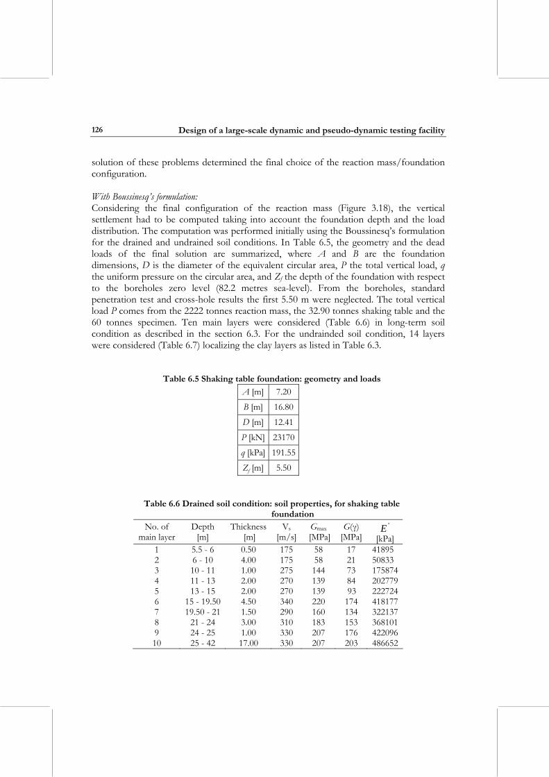
Design of a large-scale dynamic and pseudo-dynamic testing facility
126
solution of these problems determined the final choice of the reaction mass/foundation configuration. With Boussinesq’s formulation: Considering the final configuration of the reaction mass (Figure 3.18), the vertical settlement had to be computed taking into account the foundation depth and the load distribution. The computation was performed initially using the Boussinesq’s formulation for the drained and undrained soil conditions. In Table 6.5, the geometry and the dead loads of the final solution are summarized, where A and B are the foundation dimensions, D is the diameter of the equivalent circular area, P the total vertical load, q the uniform pressure on the circular area, and Zf the depth of the foundation with respect to the boreholes zero level (82.2 metres sea-level). From the boreholes, standard penetration test and cross-hole results the first 5.50 m were neglected. The total vertical load P comes from the 2222 tonnes reaction mass, the 32.90 tonnes shaking table and the 60 tonnes specimen. Ten main layers were considered (Table 6.6) in long-term soil condition as described in the section 6.3. For the undrainded soil condition, 14 layers were considered (Table 6.7) localizing the clay layers as listed in Table 6.3.
Table 6.5 Shaking table foundation: geometry and loads A [m] 7.20
B [m] 16.80
D [m] 12.41
P [kN] 23170
q [kPa] 191.55
Zf [m] 5.50
Table 6.6 Drained soil condition: soil properties, for shaking table foundation
No. of main layer
Depth [m]
Thickness [m]
Vs [m/s]
Gmax [MPa]
G(γ) [MPa]
'E [kPa]
1 5.5 - 6 0.50 175 58 17 41895 2 6 - 10 4.00 175 58 21 50833 3 10 - 11 1.00 275 144 73 175874 4 11 - 13 2.00 270 139 84 202779 5 13 - 15 2.00 270 139 93 222724 6 15 - 19.50 4.50 340 220 174 418177 7 19.50 - 21 1.50 290 160 134 322137 8 21 - 24 3.00 310 183 153 368101 9 24 - 25 1.00 330 207 176 422096 10 25 - 42 17.00 330 207 203 486652
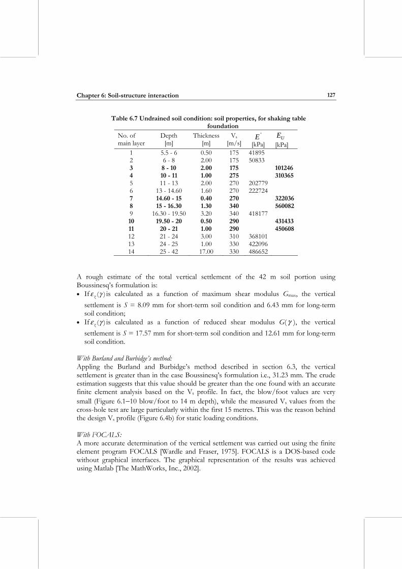
Chapter 6: Soil-structure interaction
127
Table 6.7 Undrained soil condition: soil properties, for shaking table foundation
No. of main layer
Depth [m]
Thickness [m]
Vs [m/s]
'E [kPa]
UE [kPa]
1 5.5 - 6 0.50 175 41895 2 6 - 8 2.00 175 50833 3 8 - 10 2.00 175 101246 4 10 - 11 1.00 275 310365 5 11 - 13 2.00 270 202779 6 13 - 14.60 1.60 270 222724 7 14.60 - 15 0.40 270 322036 8 15 - 16.30 1.30 340 560082 9 16.30 - 19.50 3.20 340 418177 10 19.50 - 20 0.50 290 431433 11 20 - 21 1.00 290 450608 12 21 - 24 3.00 310 368101 13 24 - 25 1.00 330 422096 14 25 - 42 17.00 330 486652
A rough estimate of the total vertical settlement of the 42 m soil portion using Boussinesq’s formulation is: • If )(γεz is calculated as a function of maximum shear modulus Gmax, the vertical
settlement is S = 8.09 mm for short-term soil condition and 6.43 mm for long-term soil condition;
• If )(γεz is calculated as a function of reduced shear modulus G(γ ), the vertical settlement is S = 17.57 mm for short-term soil condition and 12.61 mm for long-term soil condition.
With Burland and Burbidge’s method: Appling the Burland and Burbidge’s method described in section 6.3, the vertical settlement is greater than in the case Boussinesq’s formulation i.e., 31.23 mm. The crude estimation suggests that this value should be greater than the one found with an accurate finite element analysis based on the Vs profile. In fact, the blow/foot values are very small (Figure 6.1−10 blow/foot to 14 m depth), while the measured Vs values from the cross-hole test are large particularly within the first 15 metres. This was the reason behind the design Vs profile (Figure 6.4b) for static loading conditions. With FOCALS: A more accurate determination of the vertical settlement was carried out using the finite element program FOCALS [Wardle and Fraser, 1975]. FOCALS is a DOS-based code without graphical interfaces. The graphical representation of the results was achieved using Matlab [The MathWorks, Inc., 2002].
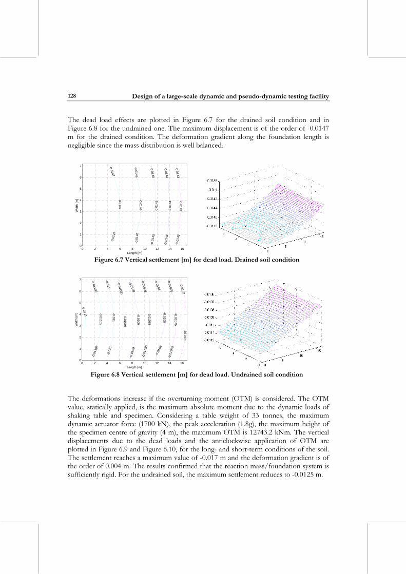
Design of a large-scale dynamic and pseudo-dynamic testing facility
128
The dead load effects are plotted in Figure 6.7 for the drained soil condition and in Figure 6.8 for the undrained one. The maximum displacement is of the order of -0.0147 m for the drained condition. The deformation gradient along the foundation length is negligible since the mass distribution is well balanced.
0 2 4 6 8 10 12 14 160
1
2
3
4
5
6
7
Length [m]
Wid
th [m
]
-0.0147
-0.0147
-0.0
147
-0.0146-0.0146
-0.0
146
-0.0145
-0. 0
1 45
-0.0
145
-0.0144
-0.0
144
-0.0
144
-0.0143-0.0143
-0.0
143
Figure 6.7 Vertical settlement [m] for dead load. Drained soil condition
0 2 4 6 8 10 12 14 160
1
2
3
4
5
6
7
Length [m]
Wid
th [m
]
-0.0111
-0.01105-0.01105
-0.0
1105
-0.011-0.011
-0.0
11
-0.01095-0.01095
-0.0109-0.0109
-0.0
109
-0.01085-0.01085
-0.0
1085
-0.0108
-0.0108
-0.0
108
-0.01075-0.010 75
-0.0
1075
-0.0107
-0.0
1 07
Figure 6.8 Vertical settlement [m] for dead load. Undrained soil condition
The deformations increase if the overturning moment (OTM) is considered. The OTM value, statically applied, is the maximum absolute moment due to the dynamic loads of shaking table and specimen. Considering a table weight of 33 tonnes, the maximum dynamic actuator force (1700 kN), the peak acceleration (1.8g), the maximum height of the specimen centre of gravity (4 m), the maximum OTM is 12743.2 kNm. The vertical displacements due to the dead loads and the anticlockwise application of OTM are plotted in Figure 6.9 and Figure 6.10, for the long- and short-term conditions of the soil. The settlement reaches a maximum value of -0.017 m and the deformation gradient is of the order of 0.004 m. The results confirmed that the reaction mass/foundation system is sufficiently rigid. For the undrained soil, the maximum settlement reduces to -0.0125 m.

Chapter 6: Soil-structure interaction
129
0 2 4 6 8 10 12 14 160
1
2
3
4
5
6
7
Length [m]
Wid
th [m
]
-0 .017
- 0. 0
1 7- 0
.01 7
-0.01 65
-0.0
1 65
-0.01 6
- 0. 0
1 6-0
.016
-0 .0 1 5 5-0.0155
-0.01 5-0.015
- 0. 0
1 5
-0 .0 1 45-0.0145
-0 .0 14
- 0.0
14- 0
.014
-0 .0 1 35-0.0135
- 0. 01 3
- 0.0
13-0
.01 3
Figure 6.9 Vertical settlement [m] for dead load and OTM due to actuator dynamic
force. Drained soil condition
0 2 4 6 8 10 12 14 160
1
2
3
4
5
6
7
Length [m]
Wid
th [m
]
-0 .0 1 2 5-0.0125
- 0.0
12- 0
. 01 2
-0 .0 1 2
-0 .0 1 1 5-0.0115
- 0.0
115
-0 .0 1 1-0.011
-0. 0
1 1
-0.01 05
-0. 0
1 05
-0.0
105
- 0. 01
-0.0
1-0
.01
-0 .0 0 9 5
- 0. 0
0 95
Figure 6.10 Vertical settlement [m] for dead load and OTM due to actuator dynamic
force. Undrained soil condition
A brief summary of the results of the vertical settlements for the case of the discarded configurations of the reaction mass (section 3.4.2) is given for completeness. The negative effects (i) of an unbalanced mass distribution, (ii) of the discontinuity in stiffness between reaction mass and foundation (due to the presence of airbags) and (iii) of the flexibility of the foundation are shown. The first configuration considered is depicted in Figure 3.20 supported by 64 air springs (248-2 model, as described in 3.5). The foundation is a rectangular concrete block, whose size is 16.8 m by 7.2 m, and its depth with respect to the borehole zero level (82.2 m sea-level) is 3.90 m. In order to reduce the flexibility of the foundation its thickness was assumed equal to 80 cm. The vertical displacements due to the dead loads are plotted in Figure 6.11. One can see a concentration of vertical deformation corresponding to the front side of the reaction block where the majority of the dead load is concentrated. The second configuration considered was the symmetric reaction mass configuration (Figure 6.19, on left) supported by 150 T29 air springs (section 3.5). Due to previously
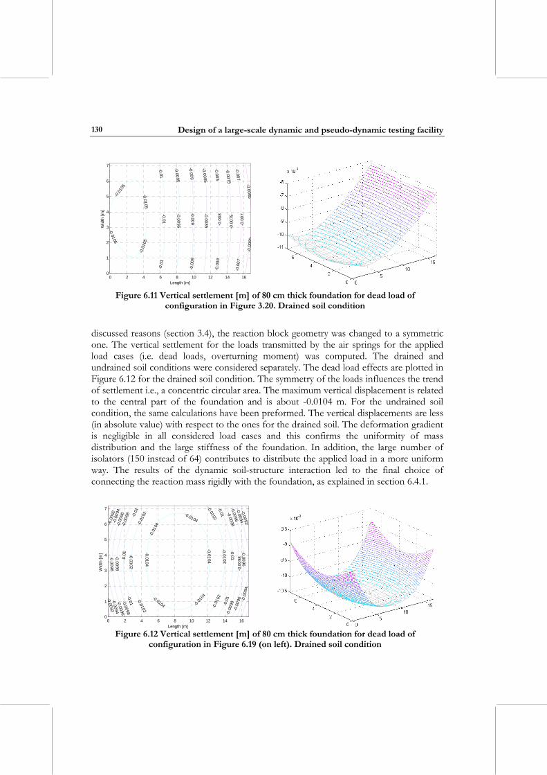
Design of a large-scale dynamic and pseudo-dynamic testing facility
130
0 2 4 6 8 10 12 14 160
1
2
3
4
5
6
7
Length [m]
Wid
th [m
]
-0.01
05
-0.0105
-0.0
105
-0.0105
-0.01-0.01
-0.0
1
-0.0095-0.0 0 95
-0.009-0.0 0 9
-0.0
09
-0.0085- 0. 00 8 5
-0.008
-0.0
0 8-0
.008
-0.0075
-0.0
0 75
-0.007
-0. 0
0 7-0
.007
-0.0065
-0.0
065
Figure 6.11 Vertical settlement [m] of 80 cm thick foundation for dead load of
configuration in Figure 3.20. Drained soil condition
discussed reasons (section 3.4), the reaction block geometry was changed to a symmetric one. The vertical settlement for the loads transmitted by the air springs for the applied load cases (i.e. dead loads, overturning moment) was computed. The drained and undrained soil conditions were considered separately. The dead load effects are plotted in Figure 6.12 for the drained soil condition. The symmetry of the loads influences the trend of settlement i.e., a concentric circular area. The maximum vertical displacement is related to the central part of the foundation and is about -0.0104 m. For the undrained soil condition, the same calculations have been preformed. The vertical displacements are less (in absolute value) with respect to the ones for the drained soil. The deformation gradient is negligible in all considered load cases and this confirms the uniformity of mass distribution and the large stiffness of the foundation. In addition, the large number of isolators (150 instead of 64) contributes to distribute the applied load in a more uniform way. The results of the dynamic soil-structure interaction led to the final choice of connecting the reaction mass rigidly with the foundation, as explained in section 6.4.1.
0 2 4 6 8 10 12 14 160
1
2
3
4
5
6
7
Length [m]
Wid
th [m
] -0.0104
-0.0104 -0.01
04
-0.0104
-0.0104
-0.01
04-0.0
102
-0.010 2
-0.0102
-0.0102
-0.01 02
-0.0
102
-0.0
1
-0.0
1
-0.01
-0.01
-0.01
-0.0
1
-0.0
098
-0.009 8-0.0098
-0.0098
-0.0
098
-0.0
098
-0.0
096
-0.009 6-0.0096
-0.0096
-0.00 96
-0.0
096
-0.0
094
-0.0094
-0.0094
-0.0
094
-0.0
092
-0.0092
-0.0092
Figure 6.12 Vertical settlement [m] of 80 cm thick foundation for dead load of
configuration in Figure 6.19 (on left). Drained soil condition
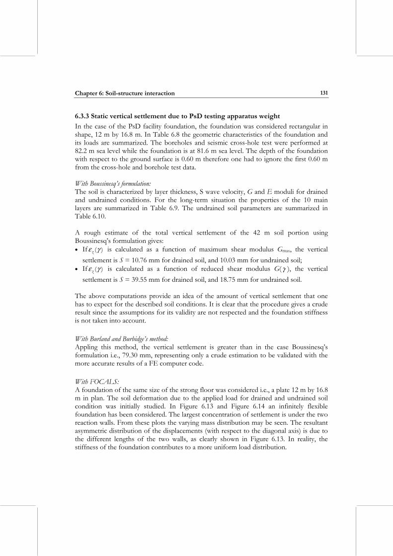
Chapter 6: Soil-structure interaction
131
6.3.3 Static vertical settlement due to PsD testing apparatus weight In the case of the PsD facility foundation, the foundation was considered rectangular in shape, 12 m by 16.8 m. In Table 6.8 the geometric characteristics of the foundation and its loads are summarized. The boreholes and seismic cross-hole test were performed at 82.2 m sea level while the foundation is at 81.6 m sea level. The depth of the foundation with respect to the ground surface is 0.60 m therefore one had to ignore the first 0.60 m from the cross-hole and borehole test data. With Boussinesq’s formulation: The soil is characterized by layer thickness, S wave velocity, G and E moduli for drained and undrained conditions. For the long-term situation the properties of the 10 main layers are summarized in Table 6.9. The undrained soil parameters are summarized in Table 6.10. A rough estimate of the total vertical settlement of the 42 m soil portion using Boussinesq’s formulation gives: • If )(γεz is calculated as a function of maximum shear modulus Gmax, the vertical
settlement is S = 10.76 mm for drained soil, and 10.03 mm for undrained soil; • If )(γεz is calculated as a function of reduced shear modulus G( γ ), the vertical
settlement is S = 39.55 mm for drained soil, and 18.75 mm for undrained soil. The above computations provide an idea of the amount of vertical settlement that one has to expect for the described soil conditions. It is clear that the procedure gives a crude result since the assumptions for its validity are not respected and the foundation stiffness is not taken into account. With Burland and Burbidge’s method: Appling this method, the vertical settlement is greater than in the case Boussinesq’s formulation i.e., 79.30 mm, representing only a crude estimation to be validated with the more accurate results of a FE computer code. With FOCALS: A foundation of the same size of the strong floor was considered i.e., a plate 12 m by 16.8 m in plan. The soil deformation due to the applied load for drained and undrained soil condition was initially studied. In Figure 6.13 and Figure 6.14 an infinitely flexible foundation has been considered. The largest concentration of settlement is under the two reaction walls. From these plots the varying mass distribution may be seen. The resultant asymmetric distribution of the displacements (with respect to the diagonal axis) is due to the different lengths of the two walls, as clearly shown in Figure 6.13. In reality, the stiffness of the foundation contributes to a more uniform load distribution.
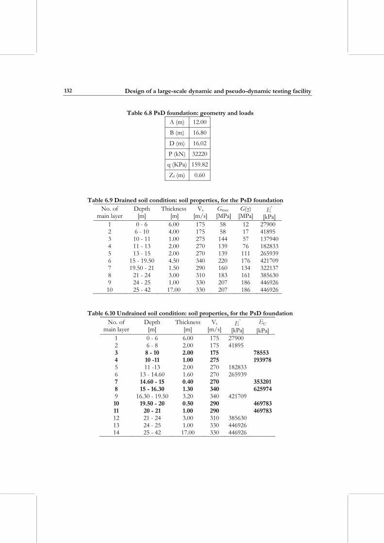
Design of a large-scale dynamic and pseudo-dynamic testing facility
132
Table 6.8 PsD foundation: geometry and loads A (m) 12.00
B (m) 16.80
D (m) 16.02
P (kN) 32220
q (KPa) 159.82
Zf (m) 0.60
Table 6.9 Drained soil condition: soil properties, for the PsD foundation No. of
main layer Depth
[m] Thickness
[m] Vs
[m/s]Gmax
[MPa]G(γ)
[MPa]'E
[kPa] 1 0 - 6 6.00 175 58 12 27900 2 6 - 10 4.00 175 58 17 41895 3 10 - 11 1.00 275 144 57 137940 4 11 - 13 2.00 270 139 76 182833 5 13 - 15 2.00 270 139 111 265939 6 15 - 19.50 4.50 340 220 176 421709 7 19.50 - 21 1.50 290 160 134 322137 8 21 - 24 3.00 310 183 161 385630 9 24 - 25 1.00 330 207 186 446926 10 25 - 42 17.00 330 207 186 446926
Table 6.10 Undrained soil condition: soil properties, for the PsD foundation No. of
main layer Depth
[m] Thickness
[m] Vs
[m/s]'E
[kPa] UE
[kPa] 1 0 - 6 6.00 175 27900 2 6 - 8 2.00 175 41895 3 8 - 10 2.00 175 78553 4 10 -11 1.00 275 1939785 11 -13 2.00 270 182833 6 13 - 14.60 1.60 270 265939 7 14.60 - 15 0.40 270 3532018 15 - 16.30 1.30 340 625974 9 16.30 - 19.50 3.20 340 421709 10 19.50 - 20 0.50 290 469783 11 20 - 21 1.00 290 469783 12 21 - 24 3.00 310 385630 13 24 - 25 1.00 330 446926 14 25 - 42 17.00 330 446926
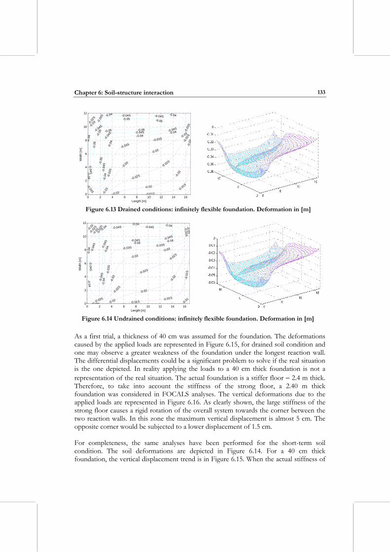
Chapter 6: Soil-structure interaction
133
0 2 4 6 8 10 12 14 160
2
4
6
8
10
12
Length [m]
Wid
th [m
] -0.0
5
-0.0
5
-0.05 -0.05
-0.05-0.05
-0.0
5
-0.045 -0.0
45-0
.045 -0.045 -0.045
-0.045-0.045
-0.045
-0.04
-0.0
4
-0.04
-0.04-0.04
-0.0
4
-0.0
4
-0.04
-0.03
5
-0.0
35
-0.035
-0.035
-0.0
35
-0.035
-0.03
-0.03
-0.03
-0.03
-0.03
-0.02
5
-0.025
-0.025
-0.02
5
-0.02
-0.02
-0.02
-0.0
2-0 015
-0.015
Figure 6.13 Drained conditions: infinitely flexible foundation. Deformation in [m]
0 2 4 6 8 10 12 14 160
2
4
6
8
10
12
Length [m]
Wid
th [m
]
- 0.04 5
-0.0
45-0
.045
-0.045 -0.045
-0.045-0.045
-0.0
45
-0.0
4
-0.04 -0.0
4-0
.04
-0.04 -0.04
-0.04-0.04
-0.04
-0.0
35 -0.035
-0.035-0.035
-0.0
35
-0.035
-0.03
-0.03
-0.03
-0.03
-0.0
3
-0 03
-0.02
5
-0.025
-0.025
-0.025
-0.02
-0.02
-0.02
-0.02
-0.015-0.015
-0.0
15
-0.01
Figure 6.14 Undrained conditions: infinitely flexible foundation. Deformation in [m]
As a first trial, a thickness of 40 cm was assumed for the foundation. The deformations caused by the applied loads are represented in Figure 6.15, for drained soil condition and one may observe a greater weakness of the foundation under the longest reaction wall. The differential displacements could be a significant problem to solve if the real situation is the one depicted. In reality applying the loads to a 40 cm thick foundation is not a representation of the real situation. The actual foundation is a stiffer floor − 2.4 m thick. Therefore, to take into account the stiffness of the strong floor, a 2.40 m thick foundation was considered in FOCALS analyses. The vertical deformations due to the applied loads are represented in Figure 6.16. As clearly shown, the large stiffness of the strong floor causes a rigid rotation of the overall system towards the corner between the two reaction walls. In this zone the maximum vertical displacement is almost 5 cm. The opposite corner would be subjected to a lower displacement of 1.5 cm. For completeness, the same analyses have been performed for the short-term soil condition. The soil deformations are depicted in Figure 6.14. For a 40 cm thick foundation, the vertical displacement trend is in Figure 6.15. When the actual stiffness of
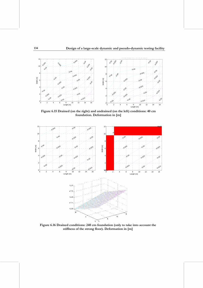
Design of a large-scale dynamic and pseudo-dynamic testing facility
134
0 2 4 6 8 10 12 14 160
2
4
6
8
10
12
Length [m]
Wid
th [m
]
-0.045
-0.045
-0.04
-0.04
-0.04
-0.04
-0.04
-0.035
-0.03
5
-0.035
-0.035
-0.035
-0.03
-0.03
-0.03
-0.03
-0.025
-0.025-0
.025
-0.02
-0.02
-0.02
-0.015
0 2 4 6 8 10 12 14 160
2
4
6
8
10
12
Length [m]
Wid
th [m
]
Vertical Settlement STRONG FLOOR
-0.0
4
-0.04
-0.04
-0.04
-0.04
-0.03
5
-0.03
5
-0.035
-0.035
-0.035
-0.03
-0.03
-0.03
-0.03
-0.03
-0.025
-0.025
-0.025
-0.02
-0.02
-0.02
-0.015
-0.01
5
-0.01
Figure 6.15 Drained (on the right) and undrained (on the left) conditions: 40 cm
foundation. Deformation in [m]
0 2 4 6 8 10 12 14 160
2
4
6
8
10
12
Length [m]
Wid
th [m
]
-0.045 -0.04
-0.04
-0.04
-0.035
-0.035
-0.035
-0.035
-0.03
-0.03
-0.03
-0.03
-0.025
-0.025
-0.025
-0.02
-0.02
-0.015
0 2 4 6 8 10 12 14 160
2
4
6
8
10
12
Length [m]
Wid
th [m
]
-0.045-0.04
-0.04
-0.04
-0.035
-0.035
-0.035
-0.035
-0.03
-0.03
-0.03
-0.03
-0.025
-0.025
-0.025
-0.02
-0.02
-0.015
Wall2
Wall1
Figure 6.16 Drained conditions: 240 cm foundation (only to take into account the
stiffness of the strong floor). Deformation in [m]
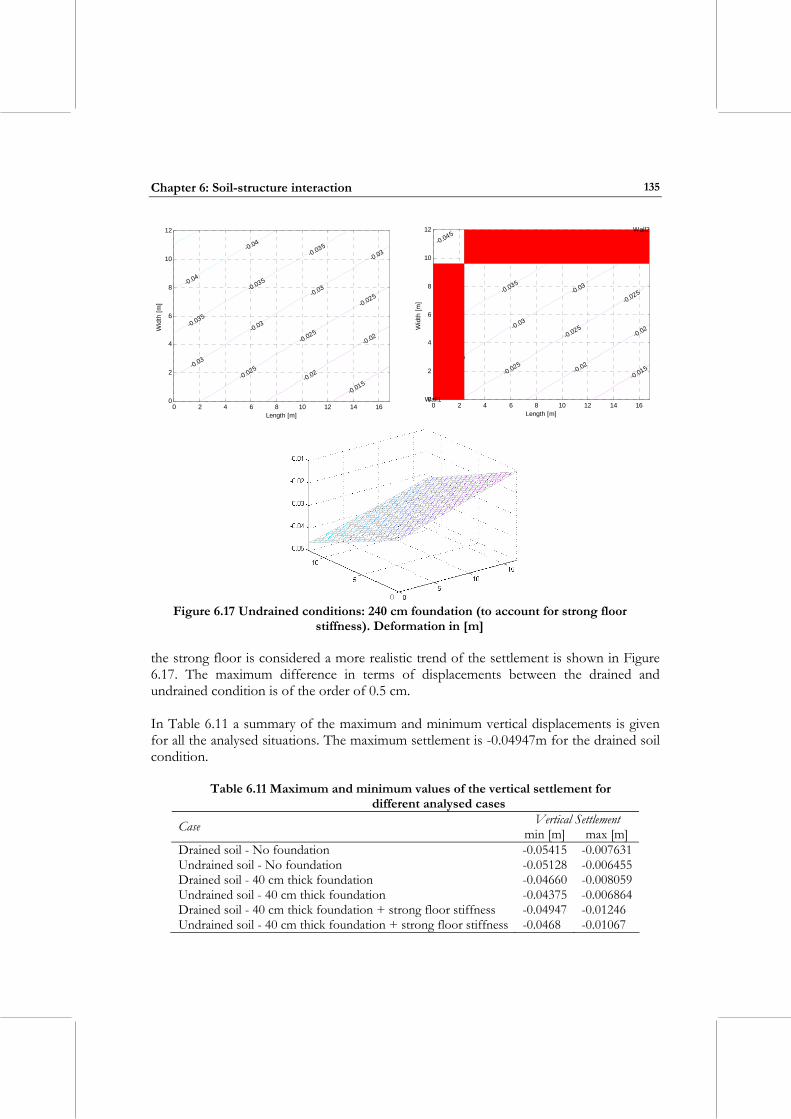
Chapter 6: Soil-structure interaction
135
0 2 4 6 8 10 12 14 160
2
4
6
8
10
12
Length [m]
Wid
th [m
]
-0.04
-0.04
-0.035
-0.035
-0.035
-0.03
-0.03
-0.03
-0.03
-0.025
-0.025
-0.025
-0.02
-0.02
-0.015
0 2 4 6 8 10 12 14 160
2
4
6
8
10
12
Length [m]W
idth
[m]
-0.045
-0.04
-0.04
-0.035
-0.035
-0.035
-0.03
-0.03
-0.03
-0.03
-0.025
-0.025
-0.025
-0.02
-0.02
-0.015
Wall2
Wall1
Figure 6.17 Undrained conditions: 240 cm foundation (to account for strong floor
stiffness). Deformation in [m]
the strong floor is considered a more realistic trend of the settlement is shown in Figure 6.17. The maximum difference in terms of displacements between the drained and undrained condition is of the order of 0.5 cm. In Table 6.11 a summary of the maximum and minimum vertical displacements is given for all the analysed situations. The maximum settlement is -0.04947m for the drained soil condition.
Table 6.11 Maximum and minimum values of the vertical settlement for different analysed cases
Vertical Settlement Case min [m] max [m] Drained soil - No foundation -0.05415 -0.007631 Undrained soil - No foundation -0.05128 -0.006455 Drained soil - 40 cm thick foundation -0.04660 -0.008059 Undrained soil - 40 cm thick foundation -0.04375 -0.006864 Drained soil - 40 cm thick foundation + strong floor stiffness -0.04947 -0.01246 Undrained soil - 40 cm thick foundation + strong floor stiffness -0.0468 -0.01067
Design of a large-scale dynamic and pseudo-dynamic testing facility
136
The rigid rotation due to the settlement of the system had to be eliminated as it could hinder the optimum performance of the facility. A preloaded condition of the soil had to be carried out to eliminate this deformation. The rigid rotation of the strong floor is caused by the unbalanced load concentration in the proximity of the two reaction walls. Before the construction of the facility, the same loads were applied on the sides opposite the final configuration of the walls. This means that the precast blocks (those that would be used to assemble the two walls) were positioned in order to produce a rigid rotation of the opposite corner.
6.4 DYNAMIC SOIL-STRUCTURE INTERACTION PROBLEM As discussed in Chapter 3, the high-performance, uniaxial shaking table under construction at EUCENTRE has forced the designers to face the challenging problem of having a large reaction mass and an expensive isolation system to control and possibly reduce the vibration impact if the traditional design approach were to be followed [Clark, 1992]. Accurate analyses must be performed in order to solve the dynamic soil-structure interaction problem. A numerical model of the specimen, shaking table, hydrostatic bearings, and reaction mass and soil/foundation system was set-up using the lumped mass approach with the aim of predicting the performance of the shaking table. Dynamic soil-foundation structure interaction was taken into account using the computer code DYNA4 [Novak et al., 1993]. A systematic numerical simulation programme was carried out using harmonic and natural excitation signals. Optimization of the reaction mass and foundation design is a result of these analyses. In this section, the methodology and the analyses are explained with reference to the work of Pavese et al. [2005]. Alongside the evaluation of acceleration, velocity and displacement values at the soil-foundation interface, an estimate of the liquefaction susceptibility of the soil has been carried out since the soil is mainly constituted by sand. Transmission of excitation from the shaking table to the ground could result in densification and consequently settlement in saturated sands. The densification of saturated sand is influenced by the density of the sand, the maximum shear strain induced in the soil, and the amount of excess pore pressure generated by the earthquake induced by the shaking table operation.
6.4.1 Dynamic soil-structure interaction For the evaluation of the dynamic response of the shaking table and foundation/soil, a three DOF lumped mass model has been developed. A rigid block placed over a deformable and dissipative ground under harmonic and transient excitations was used to model the behaviour of the dynamic testing facility (Figure 6.18).
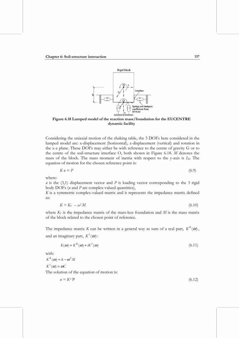
Chapter 6: Soil-structure interaction
137
Figure 6.18 Lumped model of the reaction mass/foundation for the EUCENTRE
dynamic facility
Considering the uniaxial motion of the shaking table, the 3 DOFs here considered in the lumped model are: x-displacement (horizontal), z-displacement (vertical) and rotation in the x-z plane. These DOFs may either be with reference to the centre of gravity G or to the centre of the soil-structure interface O, both shown in Figure 6.18. M denotes the mass of the block. The mass moment of inertia with respect to the y-axis is IM. The equation of motion for the chosen reference point is:
K u = P (6.9)
where: u is the (3,1) displacement vector and P is loading vector corresponding to the 3 rigid body DOFs (u and P are complex-valued quantities), K is a symmetric complex-valued matrix and it represents the impedance matrix defined as:
K = KF – ω2 M (6.10)
where KF is the impedance matrix of the mass-less foundation and M is the mass matrix of the block related to the chosen point of reference. The impedance matrix K can be written in a general way as sum of a real part, )(ωRK ,
and an imaginary part, )(ωIK :
)()()( ωωω IR iKKK += (6.11)
with: MkK R 2)( ωω −=
CK I ωω =)( The solution of the equation of motion is:
u = K-1 P (6.12)
Design of a large-scale dynamic and pseudo-dynamic testing facility
138
with amplitudes |ui|and phase angles ψi given by:
|ui|= 3,2,1,tanand)()( 22 ==+ iuuuu R
i
Ii
iIi
Ri ψ (6.13)
where Ii
Ri uu and are the real and imaginary components of the complex solution u.
The impedance matrix K is usually given with respect to the centre of the lower soil-foundation interface O whereas, the mass matrix with respect to the centre of gravity of the rigid block G. It is obvious that the equation of motion has to be established with respect to selected reference point. With reference to Eq. (6.10) and Eq. (6.11), the KF is the impedance matrix of the mass-less foundation given by:
KF = k + i ω C (6.14)
The stiffness k and damping C matrices of the Eq. (6.14) are frequency-dependent coefficients obtained using the computer code DYNA4 [Novak et al., 1993]. The program DYNA4 returns the response of rigid foundations to all types of dynamic loads. The foundation stiffness and the damping constants (referred to the centre of gravity of the footing specified in the input, and then stored in matrices) are also returned for soil-structure interaction analysis. For the case under investigation, the type of foundation defined by the program is denoted as shallow foundation resting over a “composite-medium”, i.e., the footing base rests on the surface of a shallow layer underlain by a halfspace. The layer can be considered non-uniform with linearly varying shear wave velocity. The halfspace is homogeneous and viscoelastic like the overlying layers. The footing is embedded in a stratified medium. The foundation stiffness and damping matrices are computed considering both harmonic non-quadratic loads and transient loads, within the possible operational frequency range of 0-20Hz (see Table 2.5). The results obtained from the soil-structure interaction were instrumental in choosing to design the shaking table without the isolation system. Figure 6.19 shows the layout of the two competing configurations for the shaking table with (Figure 6.19 on left) and without (Figure 6.19 on right) the isolation system. This configuration without isolation system turned out to better fulfil the design requirements and therefore it was chosen and further optimized. Hereunder a brief description of the two configurations is given.
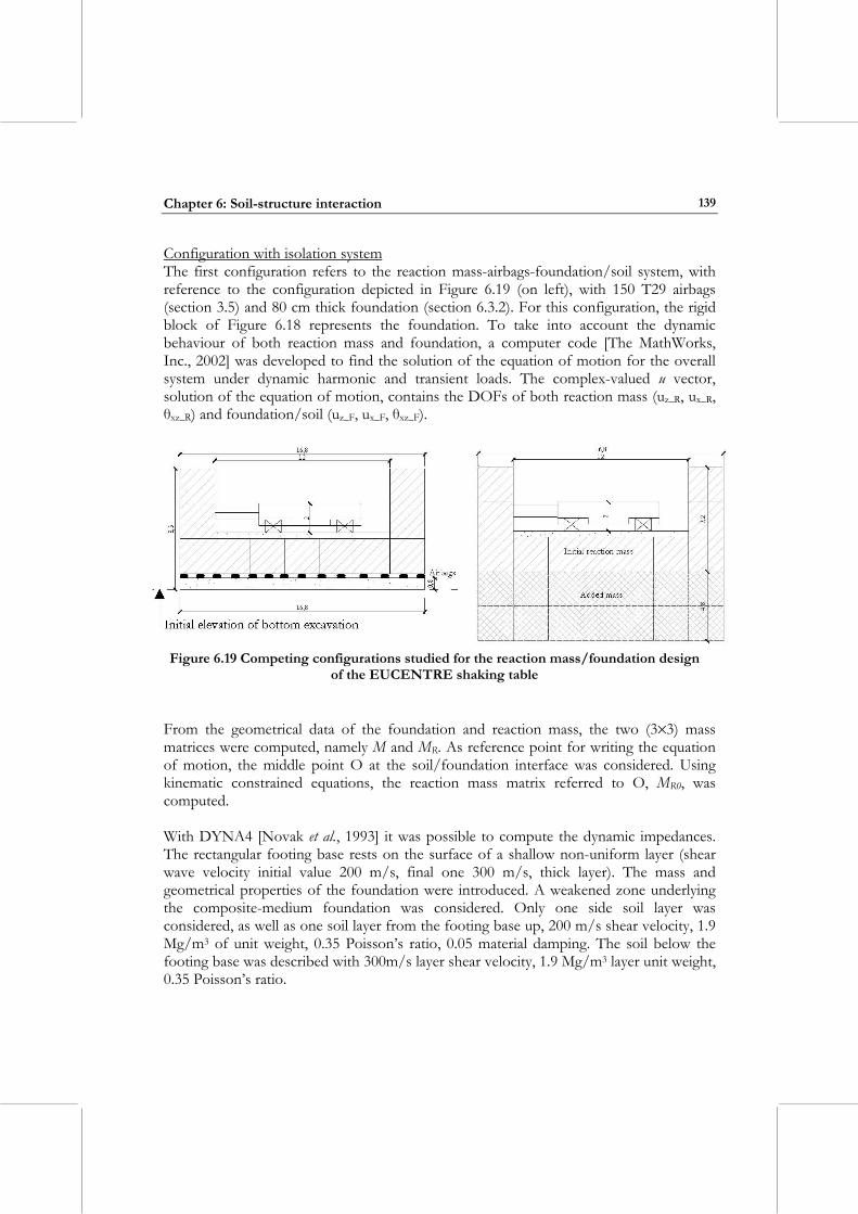
Chapter 6: Soil-structure interaction
139
Configuration with isolation system The first configuration refers to the reaction mass-airbags-foundation/soil system, with reference to the configuration depicted in Figure 6.19 (on left), with 150 T29 airbags (section 3.5) and 80 cm thick foundation (section 6.3.2). For this configuration, the rigid block of Figure 6.18 represents the foundation. To take into account the dynamic behaviour of both reaction mass and foundation, a computer code [The MathWorks, Inc., 2002] was developed to find the solution of the equation of motion for the overall system under dynamic harmonic and transient loads. The complex-valued u vector, solution of the equation of motion, contains the DOFs of both reaction mass (uz_R, ux_R, θxz_R) and foundation/soil (uz_F, ux_F, θxz_F).
Figure 6.19 Competing configurations studied for the reaction mass/foundation design of the EUCENTRE shaking table
From the geometrical data of the foundation and reaction mass, the two (3×3) mass matrices were computed, namely M and MR. As reference point for writing the equation of motion, the middle point O at the soil/foundation interface was considered. Using kinematic constrained equations, the reaction mass matrix referred to O, MR0, was computed. With DYNA4 [Novak et al., 1993] it was possible to compute the dynamic impedances. The rectangular footing base rests on the surface of a shallow non-uniform layer (shear wave velocity initial value 200 m/s, final one 300 m/s, thick layer). The mass and geometrical properties of the foundation were introduced. A weakened zone underlying the composite-medium foundation was considered. Only one side soil layer was considered, as well as one soil layer from the footing base up, 200 m/s shear velocity, 1.9 Mg/m3 of unit weight, 0.35 Poisson’s ratio, 0.05 material damping. The soil below the footing base was described with 300m/s layer shear velocity, 1.9 Mg/m3 layer unit weight, 0.35 Poisson’s ratio.
Design of a large-scale dynamic and pseudo-dynamic testing facility
140
Starting from harmonic non-quadratic loads, the defined constants were the force in x-direction (1500.9 kN) and the moment about y-axis (6999.6 kNm). As output results, the stiffness and damping constants were computed at 0.1 Hz, for vertical translation, torsion about z-axis, horizontal translation and rotation in x-z plane. The impedance matrix of the mass-less foundation, KF, is computed, as well as the impedance matrix K (Eq. (6.10)) of the soil/foundation. The local stiffness matrix of the reaction mass is computed as follows:
KRM = - ω2 MR0 (6.15)
The airbag contributions in terms of stiffness and damping were stored in two diagonal (3×3) matrices, KA and CA respectively. In terms of stiffness matrix coefficients, the total vertical, horizontal and rotational contributions were computed using the design data given by the manufacturer (vertical stiffness 1154.4 kN/m; horizontal stiffness 316 kN/m at 6 bar) [Cf_Gomma, 2001]. For the damping matrix, the design-damping ratio of the airbags (ξ≤0.03) was considered. The local stiffness and damping matrices introduced were then assembled to form the global system stiffness matrix, K. The (6×6) K matrix takes into account the 3 DOFs of the reaction mass and the 3 DOFs of the soil/foundation. The elements of rows and columns with index between 1 and 3 have been derived from the assembly of the local reaction mass stiffness matrix, Eq. (6.15). The elements of rows and columns with index between 4 and 6 represent the assemblage of the foundation impedance matrix K. The local stiffness, KA, and damping, CA, matrices due to the airbags were assembled according to the involved DOF, as well as the mixed terms coupling horizontal DOF with rotation. The damping contributions were assembled as stiffness terms: iωCA. Therefore, the equation of motion (6.12) is updated taking into account the overall assembled system:
Ka ua = Pa (6.16)
where: Ka is the assembled system matrix (6×6), ua is the (6,1) vector assembling the DOFs of reaction mass and foundation/soil, Pa is the (6,1) vector of the external dynamic loads from the reaction mass. This load vector includes the horizontal force given by the actuator, and the moment due to the horizontal force (which has a vertical arm with respect to the foundation) and the vertical reactions from the fixed basements due to the OTM of both platform and specimen. The solution of the equation of motion is the complex displacement amplitude ua of the assembled system from which displacements, accelerations for both reaction mass and foundation/soil interface, as well as foundation reactions in terms of forces and moments were computed.
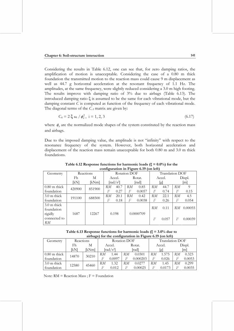
Chapter 6: Soil-structure interaction
141
Considering the results in Table 6.12, one can see that, for zero damping ratios, the amplification of motion is unacceptable. Considering the case of a 0.80 m thick foundation the transmitted motion to the reaction mass could cause 9 m displacement as well as 44.7 g horizontal acceleration at the resonant frequency of 1.1 Hz. The amplitudes, at the same frequency, were slightly reduced considering a 3.0 m high footing. The results improve with damping ratio of 3% due to airbags (Table 6.13). The introduced damping ratio ξ is assumed to be the same for each vibrational mode, but the damping constant C is computed as function of the frequency of each vibrational mode. The diagonal terms of the CA matrix are given by:
Cii = 2 ξ ωi / 2iiφ , i = 1, 2, 3 (6.17)
where iiφ are the normalized mode shapes of the system constituted by the reaction mass and airbags. Due to the imposed damping value, the amplitude is not “infinity” with respect to the resonance frequency of the system. However, both horizontal acceleration and displacement of the reaction mass remain unacceptable for both 0.80 m and 3.0 m thick foundations.
Table 6.12 Response functions for harmonic loads (ξ = 0.0%) for the configuration in Figure 6.19 (on left)
Geometry Reactions Rotation DOF Translation DOF
Fh [kN]
M [kNm]
Accel. [rad/s2]
Rotat. [rad]
Accel. [g]
Displ. [m]
RM 40.7 RM 0.85 RM 44.7 RM 9 0.80 m thick foundation 420900 851900 F 0.27 F 0.0057 F 0.74 F 0.15
RM 20.1 RM 0.42 RM 22.1 RM 4.5 3.0 m thick foundation 191100 688500 F 0.18 F 0.0038 F 0.26 F 0.054
RM 0.11 RM 0.00055 3.0 m thick foundation rigidly connected to RM
1687 12267 0.198 0.0000709 F 0.057 F 0.00039
Table 6.13 Response functions for harmonic loads (ξ = 3.0% due to
airbags) for the configuration in Figure 6.19 (on left) Geometry Reactions Rotation DOF Translation DOF
Fh [kN]
M [kNm]
Accel. [rad/s2]
Rotat. [rad]
Accel. [g]
Displ. [m]
RM 1.44 RM 0.0301 RM 1.575 RM 0.323 0.80 m thick foundation 14870 30210 F 0.0097 F 0.000203 F 0.026 F 0.0053
RM 1.32 RM 0.0277 RM 1.45 RM 0.299 3.0 m thick foundation 12580 45460 F 0.012 F 0.00025 F 0.0173 F 0.0035
Note: RM = Reaction Mass ; F = Foundation
Design of a large-scale dynamic and pseudo-dynamic testing facility
142
It should be emphasized that the kinematic response of the shaking table system could be improved (i.e. obtaining acceptable values of displacements and accelerations) by adding a set of external dampers to increase the values of damping ratio (as explained in section 3.5). The best solution should be to locate external dampers inclined at 45° in order to damp out both horizontal and vertical motions in the same way. If the airbags were discarded and a rigid connection was imposed between reaction mass and a 3.0 m thick foundation, the response was strongly reduced (Table 6.12, third case) for a resonant frequency of 7.6 Hz. Following the results in Table 6.12 for the configuration without the airbags and the external dampers, and that with an increased overall reaction mass and depth of excavation, an alternative methodology was to be adopted, i.e., no base isolation, no external dampers and relatively light reaction mass. Configuration without isolation system The second configuration refers to the rigid block formed by the reaction mass and the foundation. The initial trial configuration is depicted in Figure 6.19: 4.80 metres of concrete were added to the original precast system increasing the weight of the reaction mass up to 2680 tonnes. The computer code DYNA4 [Novak et al., 1993] was used for the new model of foundation and soil. The layer shear wave velocity was increased from 200 m/s to 300 m/s, instead 200 m/s was maintained for the side layer. The weak zone was increased, so was the excavation depth. As in the previous solution, the harmonic non-quadratic loads were defined by two amplitudes: the force in x-direction (1500.9 kN) and the moment about y-axis (6999.6 kNm). As output results, the stiffness and damping constants were computed at 0.1 Hz step, for vertical translation, torsion about z-axis, horizontal translation and rotation in x-z plane of the overall rigid block. The impedance matrix K is computed and the solved equation of motion is Eq. (6.12). The complex u contains the z-displacement, x-displacement and the rotation in the x-z plane of the rigid block. From DYNA4 the amplitudes u are computed with respect to the centre of gravity of the overall system composed by the reaction mass rigidly connected to the foundation. In order to validate the computer code developed to model the foundation/soil, a comparison was made using DYNA 4. The same analysis with harmonic non-quadratic loads was performed and the displacements and accelerations were computed at the centre of gravity of the rigid block and at its interface with the soil. Table 6.14 shows the maximum response of the rigid block. The displacements and accelerations were largely reduced with respect to the dynamic response of the base-isolated model (Figure 6.19, on left). The maximum translation of the system is 6.277E-4 m at the resonant frequency of 6.10 Hz.
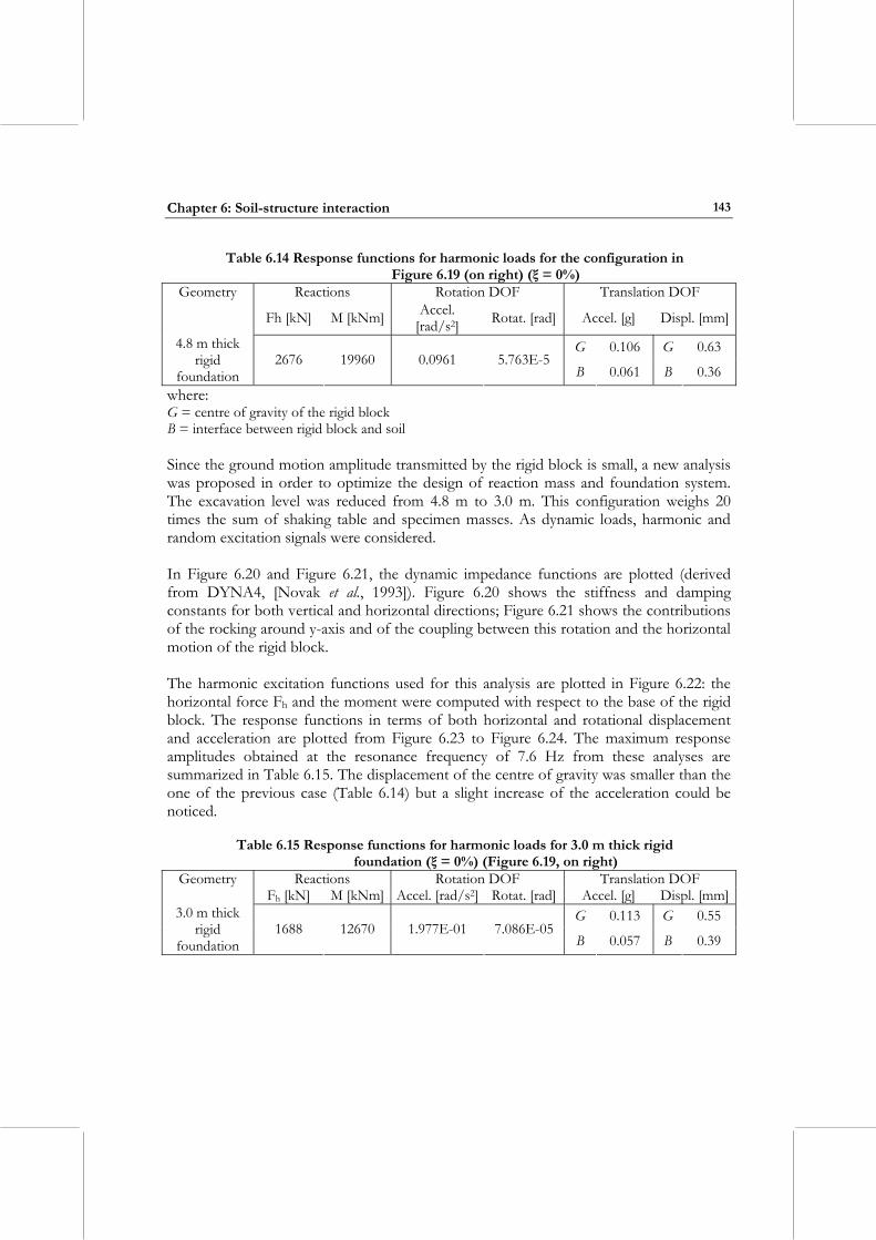
Chapter 6: Soil-structure interaction
143
Table 6.14 Response functions for harmonic loads for the configuration in Figure 6.19 (on right) (ξ = 0%)
Reactions Rotation DOF Translation DOF Geometry
Fh [kN] M [kNm] Accel. [rad/s2] Rotat. [rad] Accel. [g] Displ. [mm]
G 0.106 G 0.63 4.8 m thick rigid
foundation 2676 19960 0.0961 5.763E-5
B 0.061 B 0.36 where: G = centre of gravity of the rigid block B = interface between rigid block and soil Since the ground motion amplitude transmitted by the rigid block is small, a new analysis was proposed in order to optimize the design of reaction mass and foundation system. The excavation level was reduced from 4.8 m to 3.0 m. This configuration weighs 20 times the sum of shaking table and specimen masses. As dynamic loads, harmonic and random excitation signals were considered. In Figure 6.20 and Figure 6.21, the dynamic impedance functions are plotted (derived from DYNA4, [Novak et al., 1993]). Figure 6.20 shows the stiffness and damping constants for both vertical and horizontal directions; Figure 6.21 shows the contributions of the rocking around y-axis and of the coupling between this rotation and the horizontal motion of the rigid block. The harmonic excitation functions used for this analysis are plotted in Figure 6.22: the horizontal force Fh and the moment were computed with respect to the base of the rigid block. The response functions in terms of both horizontal and rotational displacement and acceleration are plotted from Figure 6.23 to Figure 6.24. The maximum response amplitudes obtained at the resonance frequency of 7.6 Hz from these analyses are summarized in Table 6.15. The displacement of the centre of gravity was smaller than the one of the previous case (Table 6.14) but a slight increase of the acceleration could be noticed.
Table 6.15 Response functions for harmonic loads for 3.0 m thick rigid
foundation (ξ = 0%) (Figure 6.19, on right) Reactions Rotation DOF Translation DOF Geometry
Fh [kN] M [kNm] Accel. [rad/s2] Rotat. [rad] Accel. [g] Displ. [mm]G 0.113 G 0.55 3.0 m thick
rigid foundation
1688 12670 1.977E-01 7.086E-05 B 0.057 B 0.39
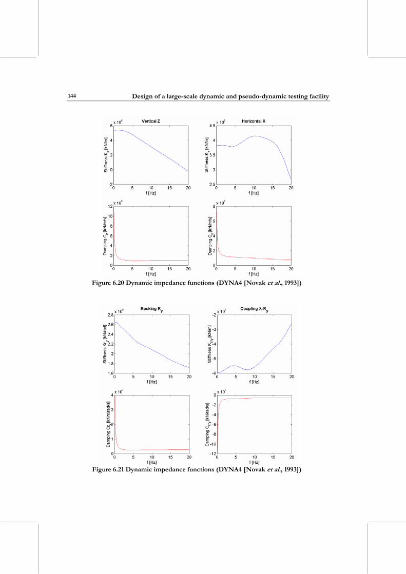
Design of a large-scale dynamic and pseudo-dynamic testing facility
144
Figure 6.20 Dynamic impedance functions (DYNA4 [Novak et al., 1993])
Figure 6.21 Dynamic impedance functions (DYNA4 [Novak et al., 1993])
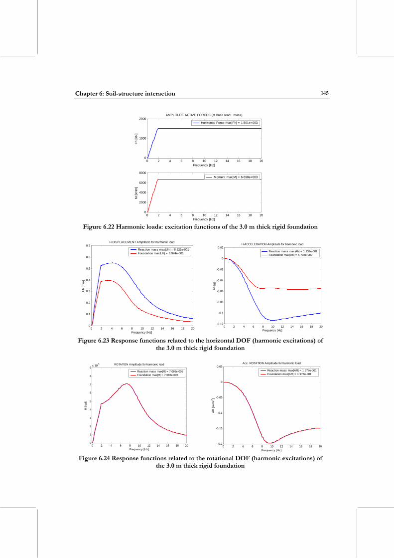
Chapter 6: Soil-structure interaction
145
0 2 4 6 8 10 12 14 16 18 200
1000
2000AMPLITUDE ACTIVE FORCES (at base react. mass)
Fh [k
N]
Frequency [Hz]
Horizontal Force max|Fh| = 1.501e+003
0 2 4 6 8 10 12 14 16 18 200
2000
4000
6000
8000
M [k
Nm
]
Frequency [Hz]
Moment max|M| = 6.698e+003
Figure 6.22 Harmonic loads: excitation functions of the 3.0 m thick rigid foundation
0 2 4 6 8 10 12 14 16 18 200
0.1
0.2
0.3
0.4
0.5
0.6
0.7H-DISPLACEMENT Amplitude for harmonic load
Uh
[mm
]
Frequency [Hz]
Reaction mass max|Uh| = 5.521e-001Foundation max|Uh| = 3.974e-001
0 2 4 6 8 10 12 14 16 18 20
-0.12
-0.1
-0.08
-0.06
-0.04
-0.02
0
0.02H-ACCELERATION Amplitude for harmonic load
Ah
[g]
Frequency [Hz]
Reaction mass max|Ah| = 1.132e-001Foundation max|Ah| = 5.708e-002
Figure 6.23 Response functions related to the horizontal DOF (harmonic excitations) of
the 3.0 m thick rigid foundation
0 2 4 6 8 10 12 14 16 18 200
1
2
3
4
5
6
7
8
9x 10⁻⁵ ROTATION Amplitude for harmonic load
R [r
ad]
Frequency [Hz]
Reaction mass max|R| = 7.086e-005Foundation max|R| = 7.086e-005
0 2 4 6 8 10 12 14 16 18 20
-0.2
-0.15
-0.1
-0.05
0
0.05Acc. ROTATION Amplitude for harmonic load
AR
[rad
/s2 ]
Frequency [Hz]
Reaction mass max|AR| = 1.977e-001Foundation max|AR| = 1.977e-001
Figure 6.24 Response functions related to the rotational DOF (harmonic excitations) of
the 3.0 m thick rigid foundation
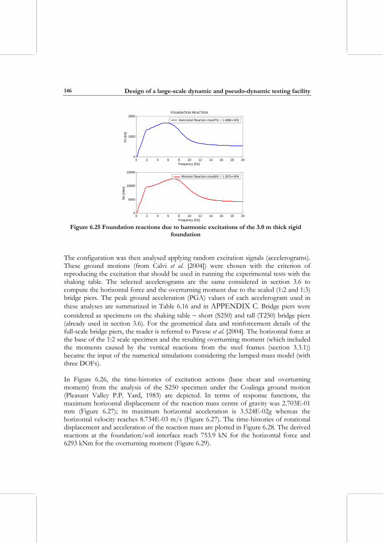
Design of a large-scale dynamic and pseudo-dynamic testing facility
146
0 2 4 6 8 10 12 14 16 18 200
1000
2000FOUNDATION REACTION
Fh [k
N]
Frequency [Hz]
Horizontal Reaction max|Fh| = 1.688e+003
0 2 4 6 8 10 12 14 16 18 200
5000
10000
15000
Mr [
kNm
]
Frequency [Hz]
Moment Reaction max|Mr| = 1.267e+004
Figure 6.25 Foundation reactions due to harmonic excitations of the 3.0 m thick rigid
foundation
The configuration was then analysed applying random excitation signals (accelerograms). These ground motions (from Calvi et al. [2004]) were chosen with the criterion of reproducing the excitation that should be used in running the experimental tests with the shaking table. The selected accelerograms are the same considered in section 3.6 to compute the horizontal force and the overturning moment due to the scaled (1:2 and 1:3) bridge piers. The peak ground acceleration (PGA) values of each accelerogram used in these analyses are summarized in Table 6.16 and in APPENDIX C. Bridge piers were considered as specimens on the shaking table − short (S250) and tall (T250) bridge piers (already used in section 3.6). For the geometrical data and reinforcement details of the full-scale bridge piers, the reader is referred to Pavese et al. [2004]. The horizontal force at the base of the 1:2 scale specimen and the resulting overturning moment (which included the moments caused by the vertical reactions from the steel frames (section 3.3.1)) became the input of the numerical simulations considering the lumped-mass model (with three DOFs). In Figure 6.26, the time-histories of excitation actions (base shear and overturning moment) from the analysis of the S250 specimen under the Coalinga ground motion (Pleasant Valley P.P. Yard, 1983) are depicted. In terms of response functions, the maximum horizontal displacement of the reaction mass centre of gravity was 2.703E-01 mm (Figure 6.27); its maximum horizontal acceleration is 3.524E-02g whereas the horizontal velocity reaches 8.734E-03 m/s (Figure 6.27). The time-histories of rotational displacement and acceleration of the reaction mass are plotted in Figure 6.28. The derived reactions at the foundation/soil interface reach 753.9 kN for the horizontal force and 6293 kNm for the overturning moment (Figure 6.29).
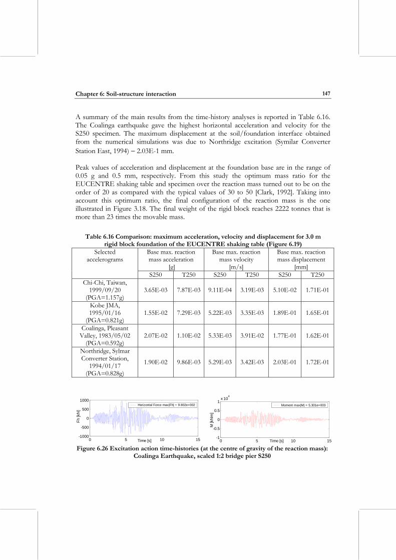
Chapter 6: Soil-structure interaction
147
A summary of the main results from the time-history analyses is reported in Table 6.16. The Coalinga earthquake gave the highest horizontal acceleration and velocity for the S250 specimen. The maximum displacement at the soil/foundation interface obtained from the numerical simulations was due to Northridge excitation (Symilar Converter Station East, 1994) − 2.03E-1 mm. Peak values of acceleration and displacement at the foundation base are in the range of 0.05 g and 0.5 mm, respectively. From this study the optimum mass ratio for the EUCENTRE shaking table and specimen over the reaction mass turned out to be on the order of 20 as compared with the typical values of 30 to 50 [Clark, 1992]. Taking into account this optimum ratio, the final configuration of the reaction mass is the one illustrated in Figure 3.18. The final weight of the rigid block reaches 2222 tonnes that is more than 23 times the movable mass.
Table 6.16 Comparison: maximum acceleration, velocity and displacement for 3.0 m
rigid block foundation of the EUCENTRE shaking table (Figure 6.19) Base max. reaction mass acceleration
[g]
Base max. reaction mass velocity
[m/s]
Base max. reaction mass displacement
[mm]
Selected accelerograms
S250 T250 S250 T250 S250 T250 Chi-Chi, Taiwan,
1999/09/20 (PGA=1.157g)
3.65E-03 7.87E-03 9.11E-04 3.19E-03 5.10E-02 1.71E-01
Kobe JMA, 1995/01/16
(PGA=0.821g) 1.55E-02 7.29E-03 5.22E-03 3.35E-03 1.89E-01 1.65E-01
Coalinga, Pleasant Valley, 1983/05/02
(PGA=0.592g) 2.07E-02 1.10E-02 5.33E-03 3.91E-02 1.77E-01 1.62E-01
Northridge, Sylmar Converter Station,
1994/01/17 (PGA=0.828g)
1.90E-02 9.86E-03 5.29E-03 3.42E-03 2.03E-01 1.72E-01
0 5 10 15-1000
-500
0
500
1000
Fh [k
N]
Time [s]
Horizontal Force max|Fh| = 9.802e+002
0 5 10 15-1
-0.5
0
0.5
1x 10
4
M [k
Nm
]
Time [s]
Moment max|M| = 5.301e+003
Figure 6.26 Excitation action time-histories (at the centre of gravity of the reaction mass): Coalinga Earthquake, scaled 1:2 bridge pier S250
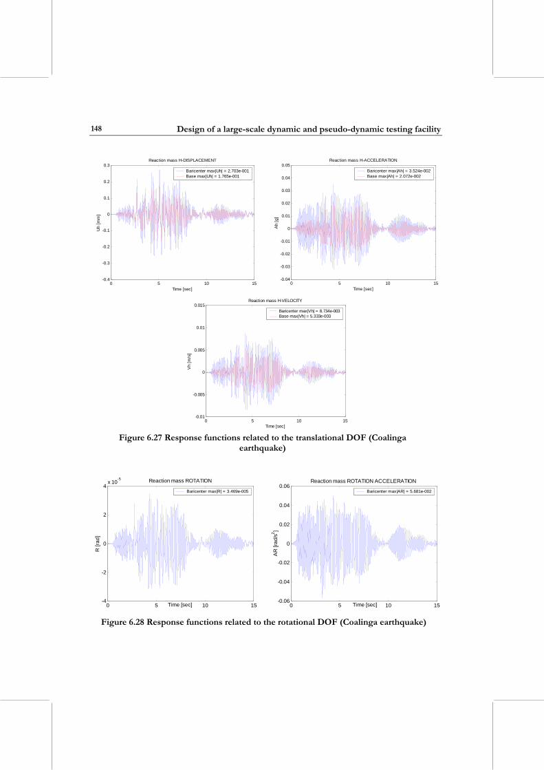
Design of a large-scale dynamic and pseudo-dynamic testing facility
148
0 5 10 15-0.4
-0.3
-0.2
-0.1
0
0.1
0.2
0.3Reaction mass H-DISPLACEMENT
Uh
[mm
]
Time [sec]
Baricenter max|Uh| = 2.703e-001Base max|Uh| = 1.765e-001
0 5 10 15
-0.04
-0.03
-0.02
-0.01
0
0.01
0.02
0.03
0.04
0.05Reaction mass H-ACCELERATION
Ah
[g]
Time [sec]
Baricenter max|Ah| = 3.524e-002Base max|Ah| = 2.072e-002
0 5 10 15-0.01
-0.005
0
0.005
0.01
0.015Reaction mass H-VELOCITY
Vh
[m/s
]
Time [sec]
Baricenter max|Vh| = 8.734e-003Base max|Vh| = 5.333e-003
Figure 6.27 Response functions related to the translational DOF (Coalinga
earthquake)
0 5 10 15-4
-2
0
2
4x 10
-5 Reaction mass ROTATION
R [r
ad]
Time [sec]
Baricenter max|R| = 3.469e-005
0 5 10 15
-0.06
-0.04
-0.02
0
0.02
0.04
0.06Reaction mass ROTATION ACCELERATION
AR
[rad
/s2 ]
Time [sec]
Baricenter max|AR| = 5.681e-002
Figure 6.28 Response functions related to the rotational DOF (Coalinga earthquake)
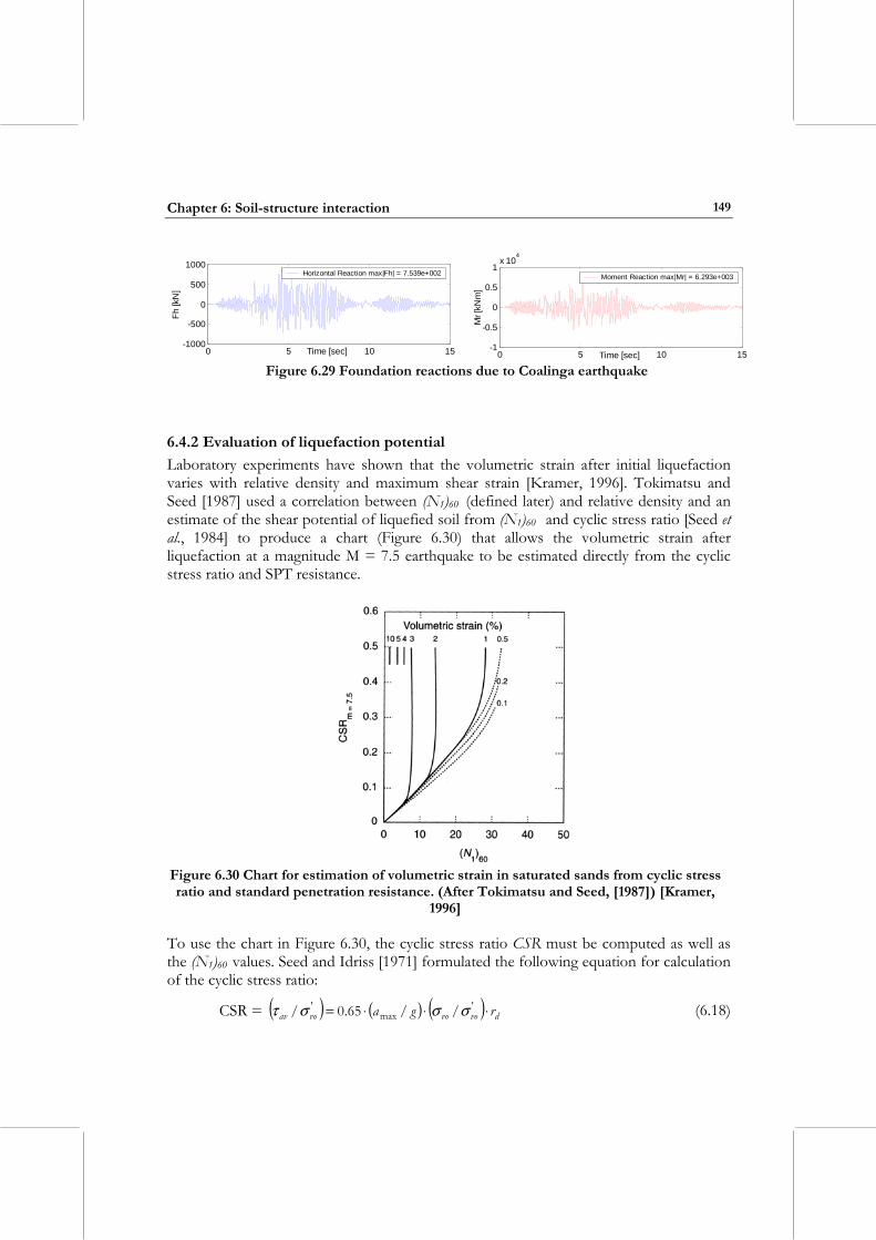
Chapter 6: Soil-structure interaction
149
0 5 10 15-1000
-500
0
500
1000
Fh [k
N]
Time [sec]
Horizontal Reaction max|Fh| = 7.539e+002
0 5 10 15-1
-0.5
0
0.5
1x 10
4
Mr [
kNm
]
Time [sec]
Moment Reaction max|Mr| = 6.293e+003
Figure 6.29 Foundation reactions due to Coalinga earthquake
6.4.2 Evaluation of liquefaction potential Laboratory experiments have shown that the volumetric strain after initial liquefaction varies with relative density and maximum shear strain [Kramer, 1996]. Tokimatsu and Seed [1987] used a correlation between (N1)60 (defined later) and relative density and an estimate of the shear potential of liquefied soil from (N1)60 and cyclic stress ratio [Seed et al., 1984] to produce a chart (Figure 6.30) that allows the volumetric strain after liquefaction at a magnitude M = 7.5 earthquake to be estimated directly from the cyclic stress ratio and SPT resistance.
Figure 6.30 Chart for estimation of volumetric strain in saturated sands from cyclic stress ratio and standard penetration resistance. (After Tokimatsu and Seed, [1987]) [Kramer,
1996]
To use the chart in Figure 6.30, the cyclic stress ratio CSR must be computed as well as the (N1)60 values. Seed and Idriss [1971] formulated the following equation for calculation of the cyclic stress ratio:
CSR = ( ) ( ) ( ) dvovovoav rga ⋅⋅⋅= 'max
' //65.0/ σσστ (6.18)
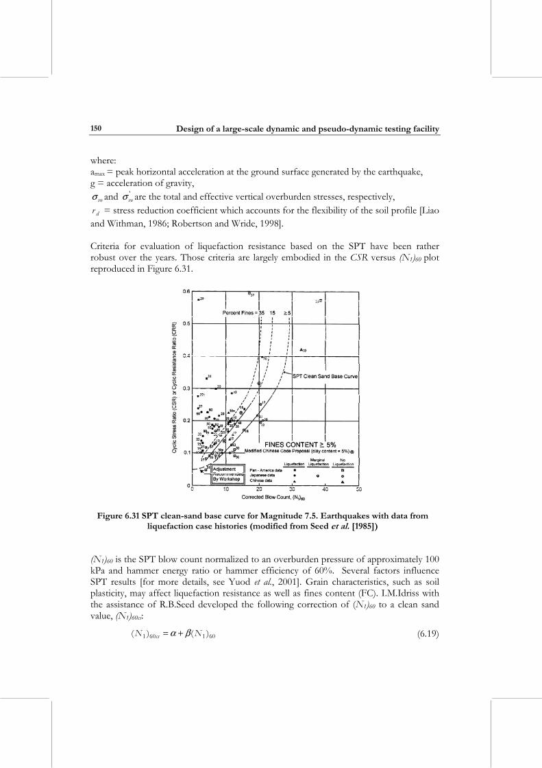
Design of a large-scale dynamic and pseudo-dynamic testing facility
150
where: amax = peak horizontal acceleration at the ground surface generated by the earthquake, g = acceleration of gravity,
voσ and 'voσ are the total and effective vertical overburden stresses, respectively,
dr = stress reduction coefficient which accounts for the flexibility of the soil profile [Liao and Withman, 1986; Robertson and Wride, 1998]. Criteria for evaluation of liquefaction resistance based on the SPT have been rather robust over the years. Those criteria are largely embodied in the CSR versus (N1)60 plot reproduced in Figure 6.31.
Figure 6.31 SPT clean-sand base curve for Magnitude 7.5. Earthquakes with data from
liquefaction case histories (modified from Seed et al. [1985])
(N1)60 is the SPT blow count normalized to an overburden pressure of approximately 100 kPa and hammer energy ratio or hammer efficiency of 60%. Several factors influence SPT results [for more details, see Yuod et al., 2001]. Grain characteristics, such as soil plasticity, may affect liquefaction resistance as well as fines content (FC). I.M.Idriss with the assistance of R.B.Seed developed the following correction of (N1)60 to a clean sand value, (N1)60cs:
601601 )()( NN cs βα += (6.19)
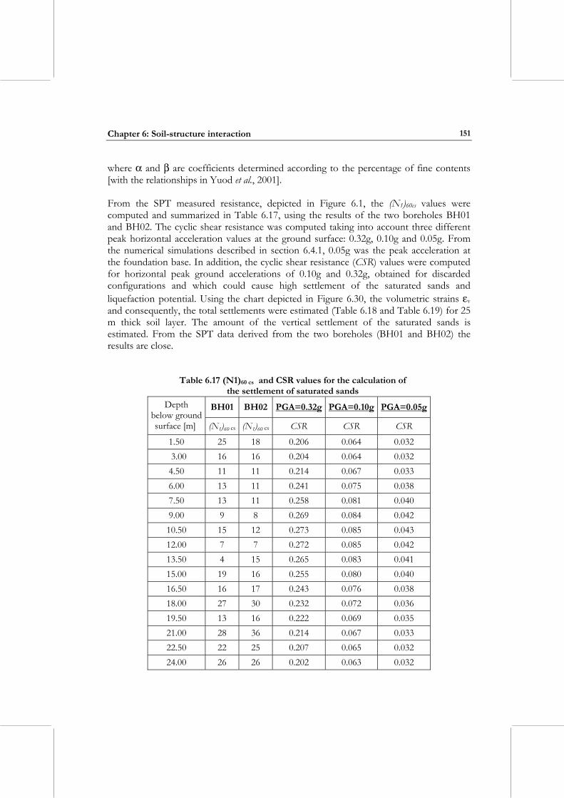
Chapter 6: Soil-structure interaction
151
where α and β are coefficients determined according to the percentage of fine contents [with the relationships in Yuod et al., 2001]. From the SPT measured resistance, depicted in Figure 6.1, the (N1)60cs values were computed and summarized in Table 6.17, using the results of the two boreholes BH01 and BH02. The cyclic shear resistance was computed taking into account three different peak horizontal acceleration values at the ground surface: 0.32g, 0.10g and 0.05g. From the numerical simulations described in section 6.4.1, 0.05g was the peak acceleration at the foundation base. In addition, the cyclic shear resistance (CSR) values were computed for horizontal peak ground accelerations of 0.10g and 0.32g, obtained for discarded configurations and which could cause high settlement of the saturated sands and liquefaction potential. Using the chart depicted in Figure 6.30, the volumetric strains εv and consequently, the total settlements were estimated (Table 6.18 and Table 6.19) for 25 m thick soil layer. The amount of the vertical settlement of the saturated sands is estimated. From the SPT data derived from the two boreholes (BH01 and BH02) the results are close.
Table 6.17 (N1)60 cs and CSR values for the calculation of the settlement of saturated sands
BH01 BH02 PGA=0.32g PGA=0.10g PGA=0.05g Depth below ground surface [m] (N1)60 cs (N1)60 cs CSR CSR CSR
1.50 25 18 0.206 0.064 0.032 3.00 16 16 0.204 0.064 0.032 4.50 11 11 0.214 0.067 0.033 6.00 13 11 0.241 0.075 0.038 7.50 13 11 0.258 0.081 0.040 9.00 9 8 0.269 0.084 0.042 10.50 15 12 0.273 0.085 0.043 12.00 7 7 0.272 0.085 0.042 13.50 4 15 0.265 0.083 0.041 15.00 19 16 0.255 0.080 0.040 16.50 16 17 0.243 0.076 0.038 18.00 27 30 0.232 0.072 0.036 19.50 13 16 0.222 0.069 0.035 21.00 28 36 0.214 0.067 0.033 22.50 22 25 0.207 0.065 0.032 24.00 26 26 0.202 0.063 0.032
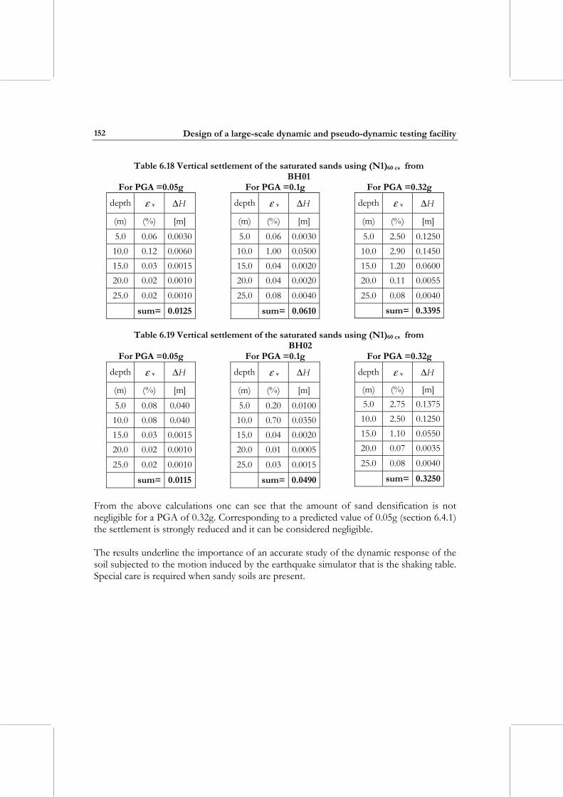
Design of a large-scale dynamic and pseudo-dynamic testing facility
152
Table 6.18 Vertical settlement of the saturated sands using (N1)60 cs from BH01
For PGA =0.05g For PGA =0.1g For PGA =0.32g
depth ε v H∆
(m) (%) [m]
5.0 0.06 0.0030 10.0 0.12 0.0060 15.0 0.03 0.0015 20.0 0.02 0.0010 25.0 0.02 0.0010
sum= 0.0125
depth ε v H∆
(m) (%) [m]
5.0 0.06 0.003010.0 1.00 0.050015.0 0.04 0.002020.0 0.04 0.002025.0 0.08 0.0040
sum= 0.0610
depth ε v H∆
(m) (%) [m]
5.0 2.50 0.1250 10.0 2.90 0.1450 15.0 1.20 0.0600 20.0 0.11 0.0055 25.0 0.08 0.0040
sum= 0.3395
Table 6.19 Vertical settlement of the saturated sands using (N1)60 cs from BH02
For PGA =0.05g For PGA =0.1g For PGA =0.32g
depth ε v H∆
(m) (%) [m]
5.0 0.08 0.040 10.0 0.08 0.040 15.0 0.03 0.0015 20.0 0.02 0.0010 25.0 0.02 0.0010
sum= 0.0115
depth ε v H∆
(m) (%) [m]
5.0 0.20 0.010010.0 0.70 0.035015.0 0.04 0.002020.0 0.01 0.000525.0 0.03 0.0015
sum= 0.0490
depth ε v H∆
(m) (%) [m] 5.0 2.75 0.1375 10.0 2.50 0.1250 15.0 1.10 0.0550 20.0 0.07 0.0035 25.0 0.08 0.0040
sum= 0.3250 From the above calculations one can see that the amount of sand densification is not negligible for a PGA of 0.32g. Corresponding to a predicted value of 0.05g (section 6.4.1) the settlement is strongly reduced and it can be considered negligible. The results underline the importance of an accurate study of the dynamic response of the soil subjected to the motion induced by the earthquake simulator that is the shaking table. Special care is required when sandy soils are present.
CHAPTER 7: CLOSURE
This manuscript described some of the work related to the design of the new EUCENTRE testing facility in Pavia, featuring powerful dynamic and a pseudo-dynamic large-scale testing apparatuses.
7.1 DESIGN OF THE TESTING FACILITY
7.1.1 Design of the shaking table The single degree of freedom EUCENTRE shaking table, currently under construction in Pavia (Italy) is characterized by a plan size of 5.6 m by 7.0 m and thickness of 1.5 m. It can reproduce strong ground motions characterized by peak velocity as high as 1.5 m/s, stroke of 1 m, and peak acceleration in excess of 1.8 g. In this work the solutions adopted for the design of the platform, reaction mass, isolation system, and foundation were presented. In particular, the methods for the optimization of the arrangements of platform and hydrostatic bearings were illustrated. Relevant issues for the design of the dynamic testing facility were listed and applied to arrive at the final configuration of the shaking table. The design of reaction mass/foundation system took into account the space constraints and the water table position. The reaction mass configuration was studied in detail to reduce the table’s resultant motion transmitted to the underlying soil.
7.1.2 Design of the PsD apparatus One of the most distinguishing characteristics of the EUCENTRE PsD testing facility is the presence of the two large reaction walls (L-shaped) allowing biaxial application of forces in the horizontal plane. The construction solution allows using the two reaction walls separately since they are not connected together. In this manuscript the design of both strong floor and reaction walls was described. The optimization of the structural configuration of the walls and floor was carried out to obtain a rigid, non-deformable testing facility. The design of the post-tensioning system of cables was also illustrated and the design of the complex foundation system was presented.
7.1.3 Soil-structure interaction problem The investigation of the soil-structure interaction represented an important aspect of the design of the overall testing facility since the EUCENTRE is located close to other laboratories with high-precision, electronic equipments. In this work, the present state of the soil was described on the basis of both laboratory and in-situ tests. The degradation of the soil properties due to the cyclic action of loads was considered in the design phase
Design of a large-scale dynamic and pseudo-dynamic testing facility
154
and described here. The computation of the settlements due to the static loads was illustrated for both shaking table and PsD foundations. Dynamic soil-structure interaction was taken into account and a systematic numerical simulation programme was carried out to predict the ground motion induced by the excitation of the table. An outcome of that study was the optimised design of the reaction mass/foundation system, i.e., a relatively light reaction mass (mass ratio for shaking table and specimen over reaction mass turned out to be on the order of 20) with no base isolation.
7.2 FUTURE WORK The future steps before the commissioning of the shaking table are calibration and tuning. The alignment of the actuator with both platform and reaction mass should be the first issue to be carefully scrutinised. Performance of the control system of the shaking table has to be investigated for specimen-table interaction; dynamic characteristics of large specimens may introduce significant force disturbances in the table. In other words, it would be inappropriate to run the table with controller tunings determined using the bare table, if good control is expected. The necessary simulation tools to identify the machine system’s behaviour require knowledge of the machine foundation, the structural system, the mechanical and hydraulic system, and the electronic feedback control, for full dynamic system’s characterization. One such cross-disciplinary tool should be developed at EUCENTRE to characterize the shaking table. This simulation model should be used both for predicting the system’s performance under the wide range of test configurations available, and for explaining and/or replicating observed behaviours. With regards to the pseudo-dynamic apparatus, calibration and tuning of the hydraulic actuators will necessarily have to be carried out. The performance of the electronic control system will also need to be investigated and compared against the design requirements.
REFERENCES A Abrams D.P. [1996] Effects of Scale and Loading Rate with Tests of Concrete and Masonry Structures, Earthquake Spectra, Vol. 12, No.1. Alga [2004] Alga Cable – T15 Post-Tensioning System, Technical Flyer, Milan, Italy. Aristizabal-Ochoa J.D. and Clark A.J. [1980] Large-Scale Earthquake Simulation Tables, Proceedings of the 7th World Conference on Earthquake Engineering, Istanbul, Turkey, Vol.7, pp.157-164. B Blakeborough A., Severn R.T. and Taylor C.A. [1986] The new UK six-axis shaking table, Proceedings of the 8th European Conference on Earthquake Engineering, Lisbon, Portugal, Vol. 4, pp. 97-100. Braja M.D. [1998] Principles of Geotechnical Engineering, Fourth Edition, International Thomson Publishing, California State University, Sacramento. BWFixatoren [2004] Serie RK for the Levelling, Adjustment and Fixation of Machinery and Other Heavy Equipment, Installation Varieties and Technical Information, Technical Flyer, Bertuch & Co GmbH Siemensstraße 15, 51381 Leverkusen, Germany. C Calvi G.M., Ceresa P., Casarotti C., Bolognini D., Auricchio F. [2004] Effects of Axial Force Variation in the Seismic Response of Bridges Isolated with Friction Pendulum Systems, Journal of Earthquake Engineering, Vol. 8, Special Issue 1, pp. 187-224. Calvi G.M., Pavese A. [2000] Valutazione della vulnerabilità sismica dei ponti, Chapter 5 of the Monograph (in Italian): Valutazione della Vulnerabilità Sismica dei Ponti di Catania, CNR-Gruppo Nazionale per la Difesa dei Terremoti, Rome, Italy. Carvalho E. [1998] Seismic testing of structures, Proceedings of the 11th European Conference on Earthquake Engineering, Paris, France, pp. 53-64. Ceresa P. [2004] Design of a dynamic and pseudo-dynamic testing facility, MsC thesis, ROSE School, Pavia, Italy.
Design of a large-scale dynamic and pseudo-dynamic testing facility
156
Chopra A.K. [2001] Dynamics of structures, Second Edition, Prentice Hall, Upper Saddle River, United States of America. Cf_Gomma [2001] Attuatori Pneumatici, Technical Flyer (in Italian), Milan, Italy. Clark A.J. [1992] Dynamic characteristics of large multiple degree of freedom shaking tables, Proceedings of the 10th World Conference on Earthquake Engineering, Madrid, Spain, pp. 2823-2828. Clark A.J. and Burton G.W. [1978] Design consideration for large shaking table systems, Proceedings of the 6th European Conference on Earthquake Engineering, Dubrovnik, Yugoslavia. Computer and Structures, Inc. [1995] SAP Nonlinear, 8.1.2 Structural Analysis Program, Berkely, California, US. Crewe A.J. [1998] The characterization and optimization of earthquake shaking table performance, PhD thesis, University of Bristol, Bristol, UK. D Das B.M. [1998] Principles of Geotechnical Engineering, Fourth edition, PWS Publishing Company, California State University, Sacramento. Department of Mechanical and Structural Engineering [2004] Materials and Structural Testing [online], Materials and Structural Testing Laboratory, University of Trento, Italy, available in URL: http://www.ing.unitn.it/dims/research_group/structural _design.php Donea J., Magonette G., Negro P., Pegon P., Pinto A. and Verzeletti G. [1996] Pseudo-dynamic Capabilities of the ELSA Laboratory for Earthquake Testing of Large Structures, Earthquake Spectra, Vol. 12, No. 1, pp. 163-180. Donea J. and Jones P.M. [1991] Experimental and Numerical Methods in Earthquake Engineering, Kluwer Academic Publishers, Netherlands. DUNLOP AIRSPRINGS [2002] Molle ad aria (cilindri flessibili), Gamma Standard a Piastre Smontabili, Dimensioni da 2” a 26”, Technical Catalouge (in Italian), Montlucon, France. E ECOEST [1997] Standardisation of shaking tables, Prenormative Research in Support of Eurocode 8, Report No. 1, Editor Crewe A.
References
157
ECOEST [1996] Experimental and numerical investigations on the seismic response of bridges and recommendations for code provisions, Prenormative Research in Support of Eurocode 8, Report No.4, Editors Calvi G..M. and Pinto P. F Fabbrocino G. and Cosenza E. [2004] Shaking Tables for Seismic Simulation overview of the CRdC-AMRA Project, Proceedings of the Workshop on Multidisciplinary Approach to Seismic Risk Problem. Sant’Angelo dei Lombardi, September 22, 2003. Università degli Studi di Napoli “Federico II”, Italy. Firestone [1997] Engineering Manual and Design Guide, Metric edition [online], Carmel, Indiana, US, Available from URL: http://www.firestoneindustrial.com. French C.W., Schultz A.E., Hajjar J.F., Shield C.K., Ernie D.W., Dexter R.J., Du D.H.-C., Olson S.A., Daugherty D.J., Wan C.P. [2004] Multi-Axis Subassemblage Testing (MAST) System: Description and Capabilities, Proceedings of the 13th World Conference Earthquake Engineering, Vancouver, British Columbia, Canada, paper 2146. G GERB Vibration Control Systems [2000] Vibration Isolation Systems, Tenth Edition, Berlin, Germany. H Hydros s.r.l. [2004] Impianto oleodinamico + Rete di distribuzione per laboratorio EUCENTRE, in Italian, Supply No. 046/04, European Centre for Training and Research, Pavia, Italy. J Joint Research Centre - ELSA [1999] The European Laboratory for Structural Assessment, Ispra, Italy. Available from the URL: http://www. elsa.jrc.it/reactionwall/index.html. K Kitada Y., Kinoshita M., Kubo T., Seo K. and Konno T. [2000] The test methodology to evaluate ultimate earthquake response of an NPP building using earthquake ground motion by blasting, Proceedings of the 12th World Conference on Earthquake Engineering, Auckland, New Zealand, paper 900. Kramer S.L. [1996] Geotechnical Earthquake Engineering, Prentice Hall, Upper Saddle River, New Jersey.
Design of a large-scale dynamic and pseudo-dynamic testing facility
158
L Lancellotta R. [1987] Geotecnica, First Edition, Zanichelli. Liao S.S.C. and Withman R.V. [1986] Catalogue of liquefaction and non-liquefaction occurrences during earthquakes. Research Report, Department of Civil Engineering, Massachusetts Institute of Technology, Cambridge, Massachusetts. M MAC Spa Modern Advanced Concrete [2002] EMACO S55 – Malta Cementizia Premiscelata per Ancoraggio. Reoplastica, a Ritiro Compensato, Technical Flyer in Italian, Treviso, Italy. Mahin S.A., Shing P.B., Thewalt C.R. and Hanson R.D. [1989] Pseudo-dynamic test method: current status and future directions, Journal of Structural Engineering, Vol. 115, pp. 2113-2128. Mahin S.A. and Shing P.B. [1985] Pseudo-dynamic method for seismic testing, Journal Structural Engineering, Vol. 111, pp. 1482-1503. Minowa C., Hayashida T., Abe I., Kida T. and Okada T. [1996] A shaking table damage test of actual size RC frame, Proceedings of the 11th World Conference on Earthquake Engineering, Acapulco, Mexico, paper 747. Molina F.J., Verzeletti G., Magonette G., Buchet P. and Geradin M. [1999] Bi-directional pseudo-dynamic test of a full-size three-storey building, Earthquake Engineering & Structural Dynamics, Vol. 28, pp. 1541-1566. MTS System Corporation [2004] EUCENTRE Uniaxial Table Testing System and Pseudo dynamic Structural Testing System, Supply No. 03252004, revision B, European Centre for Training and Research, Pavia, Italy. N Nakashima M., Kaminosono T., Ishida M. and Ando K. [1990] Integration technique for substructure pseudo-dynamic test, Proceedings of the 4th US National Conference on Earthquake Engineering, Palm Springs, pp. 515-524. Negro P., Verzeletti G., Magonette G.E. and Pinto A.V. [1994] Tests on a Four-Storey Full-Scale R/C Frame Designed According to Eurocodes 8 and 2: Preliminary Report, Research Report No. EUR 15879 EN, Joint Research Centre, Ispra, Italy. Novak M., Sheta M., El-Hifnawy L., El-Marsafawi H. and Ramadan O. [1993] DYNA4 – A Computer Program for Calculation of Foundation Response to Dynamic Loads, User Manual,
References
159
Geotechnical Research Centre, The University of Western Ontario London, Ontario, Canada. O Ogawa N., Ohtani K., Katayama T. and Shibata H. [2001] Construction of a three-dimensional large-scale shaking table and development of core technology, Philosophical Transactions of the Royal Society: mathematical, physical and engineering sciences, Vol. 359, pp. 1725-1751. Ogawa N., Ohtani K., Nakamura I., Sato E. and Nagasaki T. [2000] Development of core technology for 3D 1200 tonne large shaking table, Proceedings of the 12th World Conference on Earthquake Engineering, Auckland, New Zealand, paper 2156. Ohta T. and Goto N. [1978] Empirical Shearwave Velocity Equations in Terms of Characteristic Soil Indexes, Earthquake Engineering & Structural Dynamics, Vol. 6, pp. 167-187. Otani S. and Sozen M.A. [1972] Behavior of Multistory Reinforced Concrete Frames during Earthquakes, Research Report SRS-392, Structural Research Series, University of Illinois, Urbana, U.S. P Paulson T.J. and Abrams D.P. [1990] Correlation between Static and Dynamic Response of Model Masonry Structures, Earthquake Spectra, Vol. 6, No. 3. Pavese A., Lai C.G., Calvi G.M., Ceresa P. and Beltrami C. [2005] Reaction mass and foundation of the high-performance, one-degree-of-freedom EUCENTRE shaking table, in Pavia, Italy, Proceedings of the The First International Conference on Advances in Experimental Structural Engineering, Nagoya, Japan. Pavese A., Peloso S., Bolognini D. [2004] FRP Seismic Retrofit of RC Square Hollow Section Bridge Piers, Journal of Earthquake Engineering, Vol. 8, Special Issue 1, pp. 225-250. Pinho R. [2000] Shaking table testing of RC walls, ISET Journal of Earthquake Technology, Vol. 37, No. 4, pp. 119-142. Pinho R. and Elnashai A.S. [2000] Dynamic collapse testing of a full-scale four storey RC frame, ISET Journal of Earthquake Technology, Vol. 37, No. 4, pp. 143-164. R Robertson P.K. and Wride C.E. [1998] Evaluating cyclic liquefaction potential using the cone penetration test, Canadian Geotechnical Journal, Ottawa, Vol. 35, No. 3, pp. 442-459.
Design of a large-scale dynamic and pseudo-dynamic testing facility
160
Rogers F.J. [1908] Experiments with a shaking table, Research Report, Vol. 1, Part II, California State Earthquake Investigation Commission. S Seed H.B., Tokimatsu K., Harder L.F. and Chung R.M. [1985] The influence of SPT procedures in soil liquefaction resistance evaluation, ASCE, Journal of Geotechnical Engineering, Vol. 111, No. 12, pp. 1425-1445. Seed H.B., Wong R.T., Idriss I.M. and Tokimatsu K. [1984] Moduli and Damping Factors for Dynamic Analyses of Cohesionless Soils, ASCE, Journal of Geotechnical Engineering, Vol. 112, No. 11, pp. 1016-1032. Seed H.B. and Idriss I.M. [1971] Simplified procedure for evaluating soil liquefaction potential, ASCE, Journal of Geotechnical Engineering Division, Vol. 97, No. 9, pp. 1249-1273. Sieffert J.-G., Schmid G. and Tosecky A. [2004] Soil-Structure Interaction Foundations Vibrations, Lecture for the Master Course Computational Engineering, Rurh University Bochum, Germany. Sozen M.A., Otani S., Gulkan P. and Nielsen N.N. [1969] The University of Illinois Earthquake Simulator, Proceedings of the 4th World Conference on Earthquake Engineering, Santiago, Chile, Vol. III. Sullivan T.J., Pinho R., Pavese A. [2004] An introduction to Structural Testing Techniques in Earthquake Engineering. Educational Report No. ROSE-2004/01, IUSS Press, Pavia, Italy. T Takanashi K. and Nakashima M. [1987] Japanese activities on online testing. Journal of Engineering Mechanics, Vol. 113, pp. 1014-1032. Taucer F. and Franchioni G. [2005] Directory of European Facilities for Seismic and Dynamic Tests in Support of Industry. Cooperative Advancements in Seismic and Dynamic Experiments (CASCADE), Report No. 6. Tecno-cut [2004], Progettazione e Costruzione di una Tavola Vibrante a Sostenatamento Idrostatico, in Italian, Supply No. 2004_025 rev.3, European Centre for Training and Research, Pavia, Italy. The MathWorks, Inc. [2002] Matlab, The Language of Technical Computing, Version 6.5.0.180913a, Release 13, License Number 236982.
References
161
Thewalt C.R. and Mahin S.A. [1995] Non-planar pseudo-dynamic testing. Earthquake Engineering & Structural Dynamics, Vol. 24, pp. 733-746. Tokimatsu K. and Seed H.B. [1987] Evaluation of settlements in sand due to earthquake shaking, ASCE, Journal of Geotechnical Engineering, Vol. 113, No. 8. U University of Patras [2004] Laboratory: Structures Laboratory [online], Available from the URL: http://www.civil.upatras.gr/ V Van Den Einde L., Restrepo J., Conte J., Luco E., Seible F., Filiatrault A., Clark A., Johnson A., Gram M., Kusner D. and Thoen B. [2004] Development of the George E. Brown Jr. Network for Earthquake Engineering Simulation (NEES) Large High Performance Outdoor Shaking Table at the University of California, San Diego, Proceedings of the 13th World Conference on Earthquake Engineering, Vancouver, British Columbia, Canada, paper 3281. W Wardle L.J and Fraser R..A. [1975] Program Focals, Foundation on cross anisotropic layered system, Geomechanics computer program number 4/1, Division of applied geomechanics, Commonwealth scientific and industrial research organization, Australia. Williams M.S. and Blakeborough A. [2001] Laboratory testing of structures under dynamic loads: an introductory review, Philosophical Transactions of the Royal Society: mathematical, physical and engineering science, Vol. 359, pp. 1651-1669. Y Yuod T.L., Idriss I.M., Andrus R.D., Arango I., Castro G., Christian J.T., Dobry R., Finn W.D.L., Harder Jr. L.F., Hynes M.H., Ishihara K., Koester J.P., Liao S.S.C., Marcuson III W.F., Martin G.R., Mitchell J.K., Morawiki Y., Power M.S., Robertson P.K., Seed R.B., Stokoe II K.H. [2001] Liquefaction Resistance of Soils: Summary report from the 1996 NCEER/NSF workshops on evaluation of liquefaction resistance of soils. Journal of Geotechnical and Geoenviromental Engineering, Vol. 817.

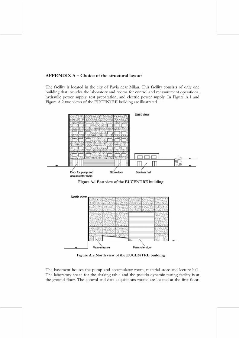
APPENDIX A – Choice of the structural layout The facility is located in the city of Pavia near Milan. This facility consists of only one building that includes the laboratory and rooms for control and measurement operations, hydraulic power supply, test preparation, and electric power supply. In Figure A.1 and Figure A.2 two views of the EUCENTRE building are illustrated.
Figure A.1 East view of the EUCENTRE building
Figure A.2 North view of the EUCENTRE building
The basement houses the pump and accumulator room, material store and lecture hall. The laboratory space for the shaking table and the pseudo-dynamic testing facility is at the ground floor. The control and data acquisitions rooms are located at the first floor.
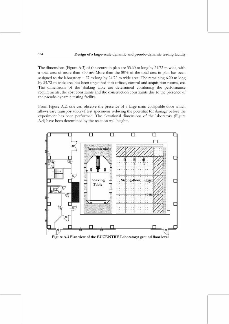
Design of a large-scale dynamic and pseudo-dynamic testing facility
164
The dimensions (Figure A.3) of the centre in plan are 33.60 m long by 24.72 m wide, with a total area of more than 830 m2. More than the 80% of the total area in plan has been assigned to the laboratory − 27 m long by 24.72 m wide area. The remaining 6.20 m long by 24.72 m wide area has been organized into offices, control and acquisition rooms, etc. The dimensions of the shaking table are determined combining the performance requirements, the cost constraints and the construction constraints due to the presence of the pseudo-dynamic testing facility. From Figure A.2, one can observe the presence of a large main collapsible door which allows easy transportation of test specimens reducing the potential for damage before the experiment has been performed. The elevational dimensions of the laboratory (Figure A.4) have been determined by the reaction wall heights.
Strong-floor Shaking Table
Reaction mass
Figure A.3 Plan view of the EUCENTRE Laboratory: ground floor level
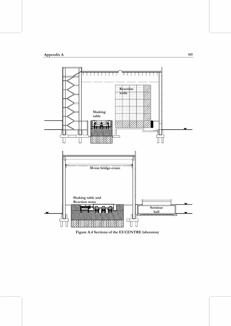
Appendix A
165
Reaction walls
Shaking table
Shaking table and Reaction mass
30-ton bridge-crane
Seminar hall
Figure A.4 Sections of the EUCENTRE laboratory

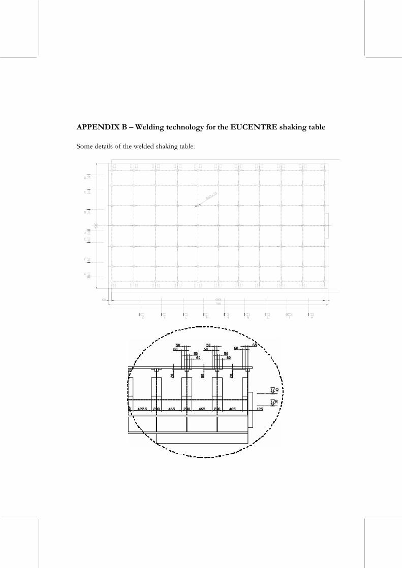
APPENDIX B – Welding technology for the EUCENTRE shaking table Some details of the welded shaking table:
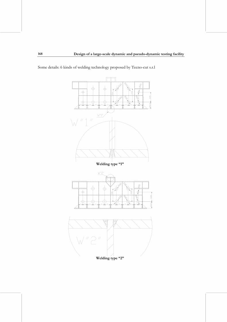
Design of a large-scale dynamic and pseudo-dynamic testing facility
168
Some details: 6 kinds of welding technology proposed by Tecno-cut s.r.l
Welding type “1”
Welding type “2”
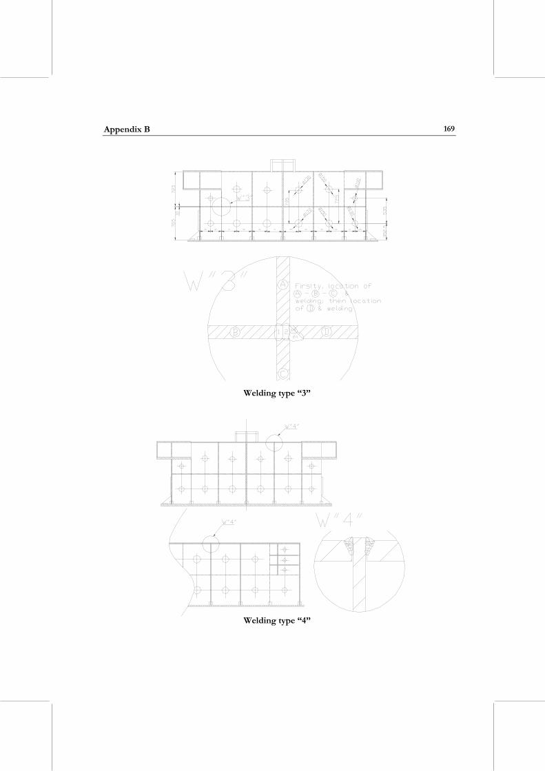
Appendix B
169
Welding type “3”
Welding type “4”
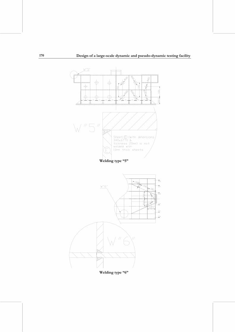
Design of a large-scale dynamic and pseudo-dynamic testing facility
170
Welding type “5”
Welding type “6”
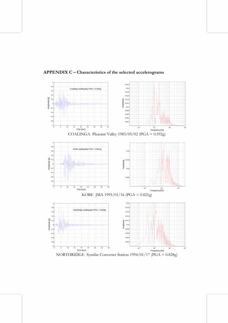
APPENDIX C – Characteristics of the selected accelerograms
0 5 10 15 20 25 30 35 40-1
-0.8
-0.6
-0.4
-0.2
0
0.2
0.4
0.6
0.8
1
Time [sec]
Am
plitu
de [g
]
Coalinga earthquake PGA = 0.592g
10-1 100 101 102
0.002
0.004
0.006
0.008
0.01
0.012
0.014
0.016
0.018
0.02
0.022
Frequency [Hz]
Am
plitu
de
COALINGA Pleasant Valley 1983/05/02 (PGA = 0.592g)
0 5 10 15 20 25 30 35 40-1
-0.8
-0.6
-0.4
-0.2
0
0.2
0.4
0.6
0.8
1
Time [sec]
Am
plitu
de [g
]
Kobe earthquake PGA = 0.821g
10-1 100 101
0.005
0.01
0.015
0.02
Frequency [Hz]
Am
plitu
de
KOBE JMA 1995/01/16 (PGA = 0.821g)
0 5 10 15 20 25 30 35 40-1
-0.8
-0.6
-0.4
-0.2
0
0.2
0.4
0.6
0.8
1
Time [sec]
Am
plitu
de [g
]
Northridge earthquake PGA = 0.828g
10-1 100 101 102
0.002
0.004
0.006
0.008
0.01
0.012
0.014
0.016
0.018
0.02
Frequency [Hz]
Am
plitu
de
NORTHRIDGE Symilar Converter Station 1994/01/17 (PGA = 0.828g)
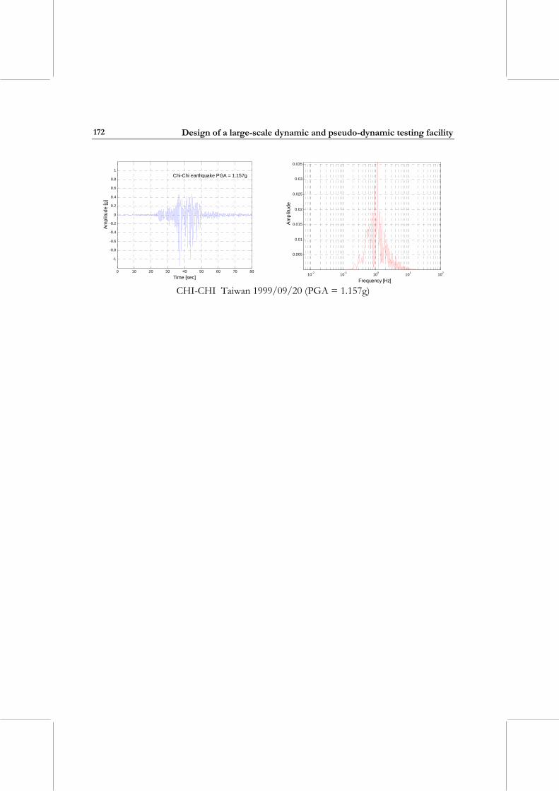
Design of a large-scale dynamic and pseudo-dynamic testing facility
172
0 10 20 30 40 50 60 70 80
-1
-0.8
-0.6
-0.4
-0.2
0
0.2
0.4
0.6
0.8
1
Time [sec]
Am
plitu
de [g
]
Chi-Chi earthquake PGA = 1.157g
10-2 10-1 100 101 102
0.005
0.01
0.015
0.02
0.025
0.03
0.035
Frequency [Hz]A
mpl
itude
CHI-CHI Taiwan 1999/09/20 (PGA = 1.157g)
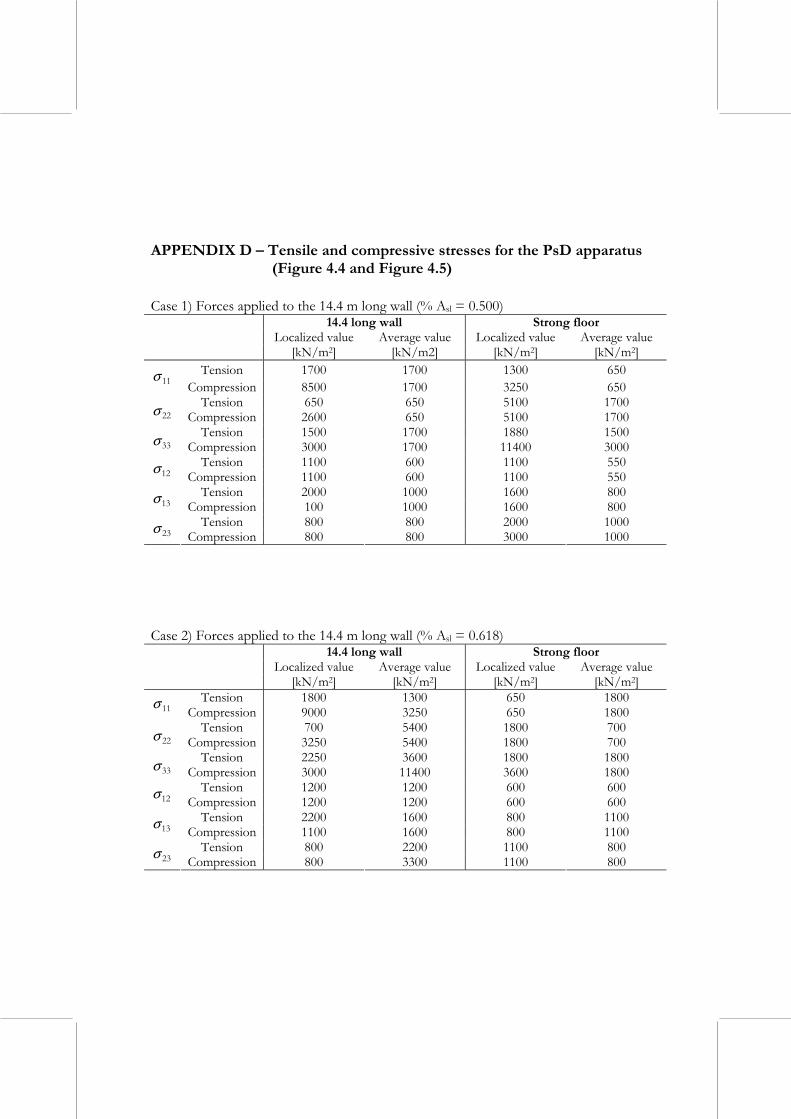
APPENDIX D – Tensile and compressive stresses for the PsD apparatus (Figure 4.4 and Figure 4.5)
Case 1) Forces applied to the 14.4 m long wall (% Asl = 0.500)
14.4 long wall Strong floor Localized value Average value Localized value Average value
[kN/m2] [kN/m2] [kN/m2] [kN/m2] Tension 1700 1700 1300 650
11σ Compression 8500 1700 3250 650
Tension 650 650 5100 1700 22σ Compression 2600 650 5100 1700
Tension 1500 1700 1880 1500 33σ Compression 3000 1700 11400 3000
Tension 1100 600 1100 550 12σ Compression 1100 600 1100 550
Tension 2000 1000 1600 800 13σ Compression 100 1000 1600 800
Tension 800 800 2000 1000 23σ Compression 800 800 3000 1000
Case 2) Forces applied to the 14.4 m long wall (% Asl = 0.618)
14.4 long wall Strong floor Localized value Average value Localized value Average value
[kN/m2] [kN/m2] [kN/m2] [kN/m2] Tension 1800 1300 650 1800
11σ Compression 9000 3250 650 1800 Tension 700 5400 1800 700
22σ Compression 3250 5400 1800 700 Tension 2250 3600 1800 1800
33σ Compression 3000 11400 3600 1800 Tension 1200 1200 600 600
12σ Compression 1200 1200 600 600 Tension 2200 1600 800 1100
13σ Compression 1100 1600 800 1100 Tension 800 2200 1100 800
23σ Compression 800 3300 1100 800
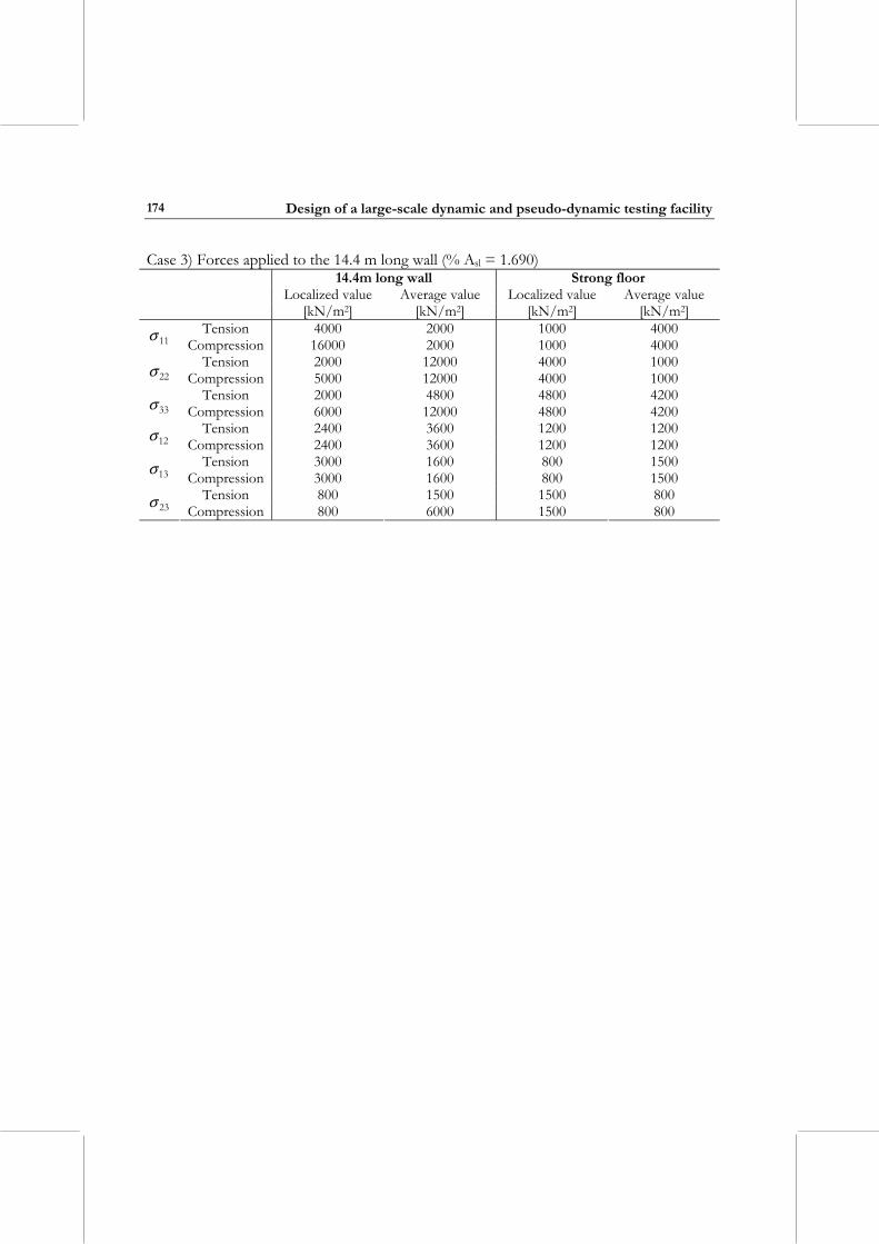
Design of a large-scale dynamic and pseudo-dynamic testing facility
174
Case 3) Forces applied to the 14.4 m long wall (% Asl = 1.690) 14.4m long wall Strong floor
Localized value Average value Localized value Average value [kN/m2] [kN/m2] [kN/m2] [kN/m2]
Tension 4000 2000 1000 4000 11σ Compression 16000 2000 1000 4000
Tension 2000 12000 4000 1000 22σ Compression 5000 12000 4000 1000
Tension 2000 4800 4800 4200 33σ Compression 6000 12000 4800 4200
Tension 2400 3600 1200 1200 12σ Compression 2400 3600 1200 1200
Tension 3000 1600 800 1500 13σ Compression 3000 1600 800 1500
Tension 800 1500 1500 800 23σ Compression 800 6000 1500 800
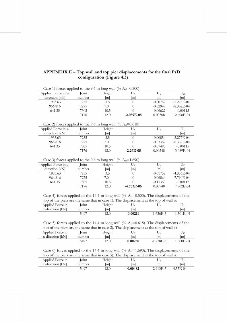
APPENDIX E – Top wall and top pier displacements for the final PsD configuration (Figure 4.3)
Case 1) forces applied to the 9.6 m long wall (% Asl=0.500)
Applied Force in y-direction [kN]
Joint number
Height [m]
UX [m]
UY [m]
UZ [m]
1933.63 7255 3.5 0 -0.00752 -5.278E-04 966.816 7275 7.0 0 -0.02949 -8.332E-04 641.35 7305 10.5 0 -0.06622 -0.00115
7176 12.0 -2.089E-05 0.00308 2.608E-04 Case 2) forces applied to the 9.6 m long wall (% Asl=0.618)
Applied Force in y-direction [kN]
Joint number
Height [m]
UX [m]
UY [m]
UZ [m]
1933.63 7255 3.5 0 -0.00854 -5.277E-04 966.816 7275 7.0 0 -0.03352 -8.332E-04 641.35 7305 10.5 0 -0.07490 -0.00115
7176 12.0 -2.26E-05 0.00348 3.089E-04 Case 3) forces applied to the 9.6 m long wall (% Asl=1.690)
Applied Force in y-direction [kN]
Joint number
Height [m]
UX [m]
UY [m]
UZ [m]
1933.63 7255 3.5 0 -0.01752 -4.356E-04 966.816 7275 7.0 0 -0.06864 -7.794E-04 641.35 7305 10.5 0 -0.15359 -0.00112
7176 12.0 -4.733E-05 0.00748 7.702E-04 Case 4) forces applied to the 14.4 m long wall (% Asl=0.500). The displacements of the top of the piers are the same that in case 1). The displacement at the top of wall is: Applied Force in x-direction [kN]
Joint number
Height [m]
UX [m]
UY [m]
UZ [m]
5497 12.0 0.00211 -1.636E-5 1.501E-04 Case 5) forces applied to the 14.4 m long wall (% Asl=0.618). The displacements of the top of the piers are the same that in case 2). The displacement at the top of wall is: Applied Force in x-direction [kN]
Joint number
Height [m]
UX [m]
UY [m]
UZ [m]
5497 12.0 0.00238 -1.778E-5 1.800E-04 Case 6) forces applied to the 14.4 m long wall (% Asl=1.690). The displacements of the top of the piers are the same that in case 3). The displacement at the top of wall is: Applied Force in x-direction [kN]
Joint number
Height [m]
UX [m]
UY [m]
UZ [m]
5497 12.0 0.00482 -2.913E-5 4.55E-04

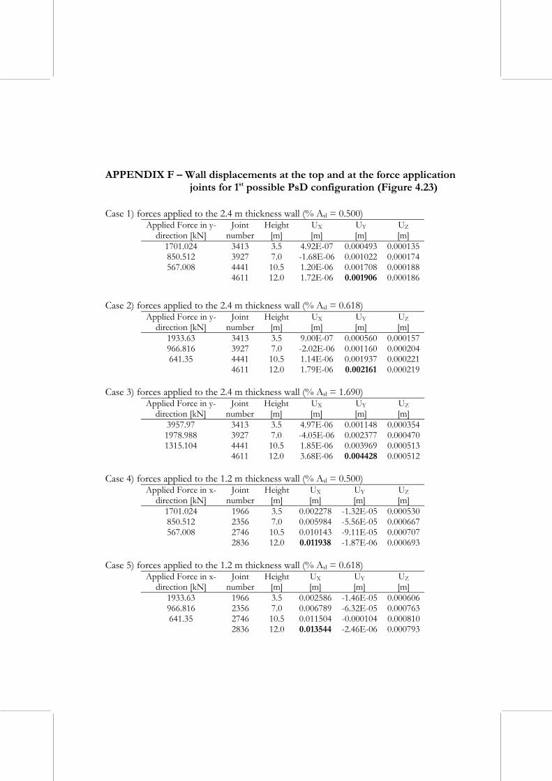
APPENDIX F – Wall displacements at the top and at the force application joints for 1st possible PsD configuration (Figure 4.23)
Case 1) forces applied to the 2.4 m thickness wall (% Asl = 0.500) Case 2) forces applied to the 2.4 m thickness wall (% Asl = 0.618)
Applied Force in y- direction [kN]
Joint number
Height [m]
UX [m]
UY [m]
UZ [m]
1933.63 3413 3.5 9.00E-07 0.000560 0.000157 966.816 3927 7.0 -2.02E-06 0.001160 0.000204 641.35 4441 10.5 1.14E-06 0.001937 0.000221
4611 12.0 1.79E-06 0.002161 0.000219 Case 3) forces applied to the 2.4 m thickness wall (% Asl = 1.690)
Applied Force in y- direction [kN]
Joint number
Height [m]
UX [m]
UY [m]
UZ [m]
3957.97 3413 3.5 4.97E-06 0.001148 0.000354 1978.988 3927 7.0 -4.05E-06 0.002377 0.000470 1315.104 4441 10.5 1.85E-06 0.003969 0.000513
4611 12.0 3.68E-06 0.004428 0.000512 Case 4) forces applied to the 1.2 m thickness wall (% Asl = 0.500)
Applied Force in x- direction [kN]
Joint number
Height [m]
UX [m]
UY [m]
UZ [m]
1701.024 1966 3.5 0.002278 -1.32E-05 0.000530 850.512 2356 7.0 0.005984 -5.56E-05 0.000667 567.008 2746 10.5 0.010143 -9.11E-05 0.000707
2836 12.0 0.011938 -1.87E-06 0.000693 Case 5) forces applied to the 1.2 m thickness wall (% Asl = 0.618)
Applied Force in x- direction [kN]
Joint number
Height [m]
UX [m]
UY [m]
UZ [m]
1933.63 1966 3.5 0.002586 -1.46E-05 0.000606 966.816 2356 7.0 0.006789 -6.32E-05 0.000763 641.35 2746 10.5 0.011504 -0.000104 0.000810
2836 12.0 0.013544 -2.46E-06 0.000793
Applied Force in y- direction [kN]
Joint number
Height [m]
UX [m]
UY [m]
UZ [m]
1701.024 3413 3.5 4.92E-07 0.000493 0.000135 850.512 3927 7.0 -1.68E-06 0.001022 0.000174 567.008 4441 10.5 1.20E-06 0.001708 0.000188
4611 12.0 1.72E-06 0.001906 0.000186

Design of a large-scale dynamic and pseudo-dynamic testing facility
178
Case 6) forces applied to the 1.2 m thickness wall (% Asl = 1.690) Applied Force in x-
direction [kN] Joint
numberHeight
[m] UX [m]
UY [m]
UZ [m]
3957.97 1966 3.5 0.005297 -2.58E-05 0.001272 1978.988 2356 7.0 0.013907 -0.000128 0.001616 1315.104 2746 10.5 0.023566 -0.000128 0.001722
2836 12.0 0.027741 -4.22E-06 0.001685

