Molecular dynamics tutorial with applications to aqueous systems

Garold Murdachaew

1400-1600, 13-14 October 2015

Chemicum A122

1

Outline

Why should I learn about molecular simulations?

Why should I learn about aqueous systems?

CP2K package for molecular simulations

VMD package for molecular visualization and analysis

gnuplot and bash scripts and fortran codes for analysis of MD trajectories

Hands-on MD exercises at CSC (taito) and on your local linux machine using

CP2K and VMD

2

Why should I learn about molecular simulations?

Another tool in your toolbox to study systems more complex than clusters

Simulations are computer experiments

Simulations allow one to see atomic detail and discover reaction mechanisms

Simulations allow one to model difficult conditions or processes:

not possible in lab (e.g., high P, high T, etc.)

too dangerous (e.g., deactivation/breakdown of nerve agents)

too expensive

Always keep in mind:

“The purpose of computing is insight, not numbers.”

– Richard Hamming, Numerical Methods for Scientists and Engineers

3

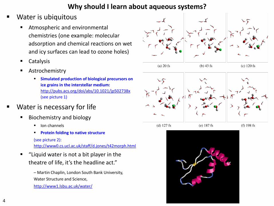
Why should I learn about aqueous systems?

Water is ubiquitous

Atmospheric and environmental

chemistries (one example: molecular

adsorption and chemical reactions on wet

and icy surfaces can lead to ozone holes)

Catalysis

Astrochemistry

Simulated production of biological precursors on

ice grains in the interstellar medium:

http://pubs.acs.org/doi/abs/10.1021/jp502738x

(see picture 1)

Water is necessary for life

Biochemistry and biology

Ion channels

Protein folding to native structure

(see picture 2):

http://www0.cs.ucl.ac.uk/staff/d.jones/t42morph.html

“Liquid water is not a bit player in the

theatre of life, it’s the headline act.”

– Martin Chaplin, London South Bank University,

Water Structure and Science,

http://www1.lsbu.ac.uk/water/

4

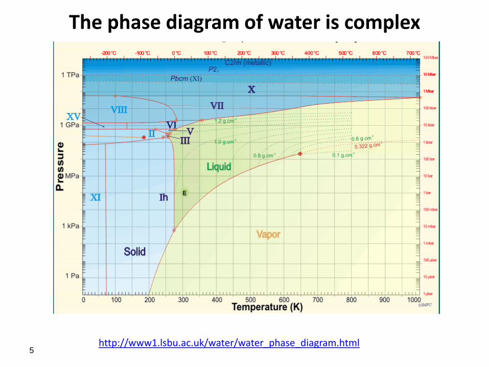
The phase diagram of water is complex

http://www1.lsbu.ac.uk/water/water_phase_diagram.html

5

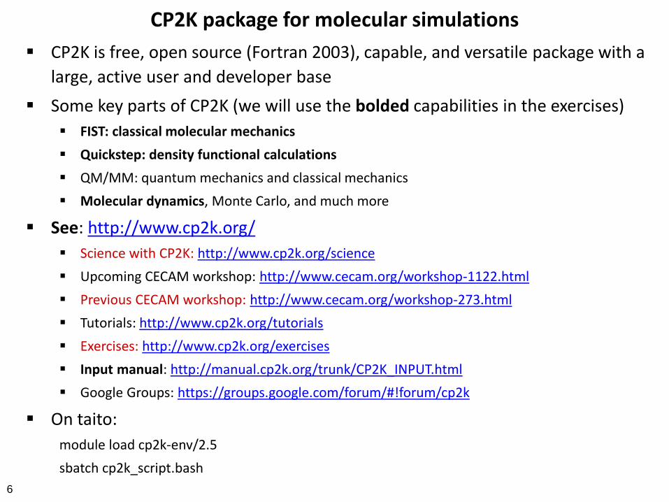
CP2K package for molecular simulations

CP2K is free, open source (Fortran 2003), capable, and versatile package with a

large, active user and developer base

Some key parts of CP2K (we will use the bolded capabilities in the exercises)

FIST: classical molecular mechanics

Quickstep: density functional calculations

QM/MM: quantum mechanics and classical mechanics

Molecular dynamics, Monte Carlo, and much more

See: http://www.cp2k.org/

Science with CP2K: http://www.cp2k.org/science

Upcoming CECAM workshop: http://www.cecam.org/workshop-1122.html

Previous CECAM workshop: http://www.cecam.org/workshop-273.html

Tutorials: http://www.cp2k.org/tutorials

Exercises: http://www.cp2k.org/exercises

Input manual: http://manual.cp2k.org/trunk/CP2K_INPUT.html

Google Groups: https://groups.google.com/forum/#!forum/cp2k

On taito:

module load cp2k-env/2.5

sbatch cp2k_script.bash

6

VMD package for molecular visualization & analysis VMD is free to download

Can be used for visualization and also analysis (gpu acceleration possible)

Can handle large systems and long trajectories in many formats (xyz, etc.)

Can produce publication quality snapshots and movies in many popular formats

Can be run interactively or using a script

See: http://www.ks.uiuc.edu/Research/vmd/

Tutorials: http://www.ks.uiuc.edu/Research/vmd/current/docs.html#tutorials

Documentation: http://www.ks.uiuc.edu/Research/vmd/current/docs.html

Mailing list for questions: http://www.ks.uiuc.edu/Research/vmd/mailing_list/vmd-l/

On taito:

module load vmd

vmd system.xyz

or

vmd -e vmd_script.vmd

7

Exercises Hands-on exercises at CSC (taito) and on your local linux machine (ask if you

wish to run locally) using CP2K and VMD. (Note that all examples are already

equilibrated but you should confirm this.)

Structure and dynamics of ambient bulk liquid water using—

Example 1: Classical potential (exercise4)

Example 2: Density functional theory (exercise5)

Calculate: Internal energy (enthalpy); Structure (RDFs); Diffusion coefficient (Einstein

relation); IR spectrum. Compare to experiment.

Example 3: Rare instance of formic acid dissociation at the air-water

interface studied with DFT (exercise6)

Timescale of deprotonation; Grotthus migration of the proton defect; Mechanisms; RDFs.

Extra examples (ask if interested): Minimum energy structures of water

clusters (H2O)n=1-21 from density functional theory; Sulfuric acid deprotonation

on wet quartz surface using DFT; etc.

8

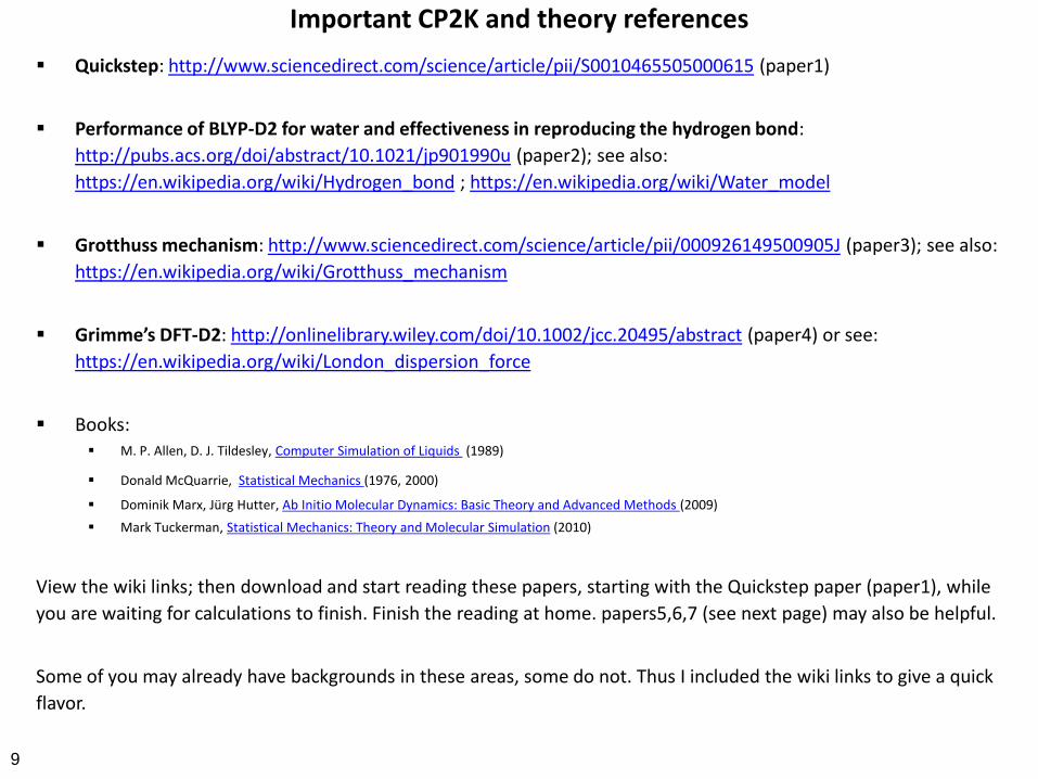
Important CP2K and theory references

Quickstep: http://www.sciencedirect.com/science/article/pii/S0010465505000615 (paper1)

Performance of BLYP-D2 for water and effectiveness in reproducing the hydrogen bond:

http://pubs.acs.org/doi/abstract/10.1021/jp901990u (paper2); see also:

https://en.wikipedia.org/wiki/Hydrogen_bond ; https://en.wikipedia.org/wiki/Water_model

Grotthuss mechanism: http://www.sciencedirect.com/science/article/pii/000926149500905J (paper3); see also:

https://en.wikipedia.org/wiki/Grotthuss_mechanism

Grimme’s DFT-D2: http://onlinelibrary.wiley.com/doi/10.1002/jcc.20495/abstract (paper4) or see:

https://en.wikipedia.org/wiki/London_dispersion_force

Books: M. P. Allen, D. J. Tildesley, Computer Simulation of Liquids (1989)

Donald McQuarrie, Statistical Mechanics (1976, 2000) Dominik Marx, Jürg Hutter, Ab Initio Molecular Dynamics: Basic Theory and Advanced Methods (2009)

Mark Tuckerman, Statistical Mechanics: Theory and Molecular Simulation (2010)

View the wiki links; then download and start reading these papers, starting with the Quickstep paper (paper1), while

you are waiting for calculations to finish. Finish the reading at home. papers5,6,7 (see next page) may also be helpful.

Some of you may already have backgrounds in these areas, some do not. Thus I included the wiki links to give a quick

flavor.

9

Recent publications from Halonen group using CP2K Relevant papers:

Relevant to Examples 1 and 2: Simulated with semiempirical method (NDDO): “Semiempirical

Self-Consistent Polarization Description of Bulk Water, the Liquid-Vapor Interface, and Cubic Ice”

http://pubs.acs.org/doi/abs/10.1021/jp110481m (paper5)

Relevant to Example 3: Simulated with DFT and shows acid deprotonation and Grotthus

mechanism: “Dissociation of HCl into Ions on Wet Hydroxylated (0001) α-Quartz”

http://pubs.acs.org/doi/abs/10.1021/jz4017969 (paper6)

Relevant to Example 3: Simulated with classical potentials and shows molecular scattering :

“Nitrogen dioxide at the air–water interface: trapping, absorption, and solvation in the bulk and at

the surface” http://pubs.rsc.org/en/content/articlehtml/2012/cp/c2cp42810e (paper7)

Other papers:

Ice slab and proton hopping example using DFT from Sampsa Riikonen: “Ionization of Acids on the

Quasi-Liquid Layer of Ice” http://pubs.acs.org/doi/abs/10.1021/jp505627n

Simulated with DFT and shows acid deprotonation and Grotthus mechanism: “First and second

deprotonation of H2SO4 on wet hydroxylated (0001) α-quartz”

http://pubs.rsc.org/en/content/articlehtml/2014/cp/c4cp02752c

10

CP2K example 1: Water with classical potential @SET BASE_NAME run

@SET ID 01

&GLOBAL

PROJECT liq

PREFERRED_FFT_LIBRARY FFTW

PRINT_LEVEL LOW

RUN_TYPE GEOMETRY_OPTIMIZATION

&END GLOBAL

&MOTION

&GEO_OPT

TYPE minimization

OPTIMIZER BFGS

MAX_ITER 400 ! 200 is default

&END GEO_OPT

&END MOTION

&FORCE_EVAL

METHOD FIST

&MM

&POISSON

&EWALD

EWALD_TYPE spme

ALPHA .44

GMAX 25 25 25

O_SPLINE 6

&END EWALD

&END POISSON

&FORCEFIELD

&SPLINE

EMAX_ACCURACY 500.0

EMAX_SPLINE 1.0E15 ! 10000000000.0

EPS_SPLINE 1.0E-9

&END SPLINE

&BEND

ATOMS H O H

K 0.

THETA0 1.8

&END BEND

&BEND

ATOMS O H H

K 0.

THETA0 1.8

&END BEND

&BOND

ATOMS O H

K 0.

R0 1.8

&END BOND

&BOND

ATOMS H H

K 0.

R0 1.8

&END BOND

&CHARGE

ATOM O

CHARGE -0.8476

&END CHARGE

&CHARGE

ATOM H

CHARGE 0.4238

&END CHARGE

11

&NONBONDED

&LENNARD-JONES

ATOMS O O

EPSILON 78.198 ! this is K, = 0.155 kcal/mol = 0.650 kJ/mol

SIGMA 3.166

RCUT 11.4

&END LENNARD-JONES

&LENNARD-JONES

ATOMS O H

EPSILON 0.0

SIGMA 3.6705

RCUT 11.4

&END LENNARD-JONES

&LENNARD-JONES

ATOMS H H

EPSILON 0.0

SIGMA 3.30523

RCUT 11.4

&END LENNARD-JONES

&END NONBONDED

&END FORCEFIELD

&END MM

&SUBSYS

&SUBSYS

&CELL

ABC 12.4138 12.4138 12.4138

&END CELL

&COORD

O 12.25967785390 1.34872474190 12.42975017890 H2O

H 12.28658481340 1.45497852510 11.43794042330 H2O

H 12.12685964540 2.28501721350 12.78165108500 H2O

...

H 10.52064998830 9.65806143920 9.70630308870 H2O

&END COORD

&TOPOLOGY

&GENERATE

! BONDLENGTH_MAX 2.0

BONDPARM_FACTOR 0.9

&END GENERATE

&END TOPOLOGY

&KIND O

ELEMENT O

&END KIND

&KIND H

ELEMENT H

&END KIND

&PRINT

&CELL

&END CELL

&END PRINT

&END SUBSYS

&PRINT

&GRID_INFORMATION

&END GRID_INFORMATION

&END PRINT

&END FORCE_EVAL

!&EXT_RESTART

! RESTART_FILE_NAME ./run-01.restart

!&END EXT_RESTART

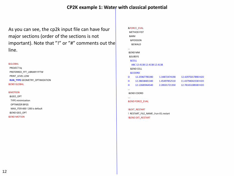
CP2K example 1: Water with classical potential

As you can see, the cp2k input file can have four

major sections (order of the sections is not

important). Note that ”!” or ”#” comments out the

line.

&GLOBAL

PROJECT liq

PREFERRED_FFT_LIBRARY FFTW

PRINT_LEVEL LOW

RUN_TYPE GEOMETRY_OPTIMIZATION

&END GLOBAL

&MOTION

&GEO_OPT

TYPE minimization

OPTIMIZER BFGS

MAX_ITER 400 ! 200 is default

&END GEO_OPT

&END MOTION

12

&FORCE_EVAL

METHOD FIST

&MM

&POISSON

&EWALD

…

&END MM

&SUBSYS

&CELL

ABC 12.4138 12.4138 12.4138

&END CELL

&COORD

O 12.25967785390 1.34872474190 12.42975017890 H2O

H 12.28658481340 1.45497852510 11.43794042330 H2O

H 12.12685964540 2.28501721350 12.78165108500 H2O

…

&END COORD

….

&END FORCE_EVAL

!&EXT_RESTART

! RESTART_FILE_NAME ./run-01.restart

!&END EXT_RESTART

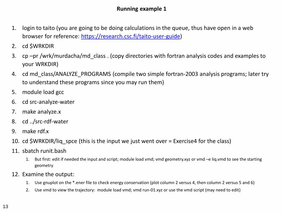
Running example 1

1. login to taito (you are going to be doing calculations in the queue, thus have open in a web

browser for reference: https://research.csc.fi/taito-user-guide)

2. cd $WRKDIR

3. cp –pr /wrk/murdacha/md_class . (copy directories with fortran analysis codes and examples to

your WRKDIR)

4. cd md_class/ANALYZE_PROGRAMS (compile two simple fortran-2003 analysis programs; later try

to understand these programs since you may run them)

5. module load gcc

6. cd src-analyze-water

7. make analyze.x

8. cd ../src-rdf-water

9. make rdf.x

10. cd $WRKDIR/liq_spce (this is the input we just went over = Exercise4 for the class)

11. sbatch runit.bash

1. But first: edit if needed the input and script; module load vmd; vmd geometry.xyz or vmd –e liq.vmd to see the starting

geometry

12. Examine the output:

1. Use gnuplot on the *.ener file to check energy conservation (plot column 2 versus 4, then column 2 versus 5 and 6)

2. Use vmd to view the trajectory: module load vmd; vmd run-01.xyz or use the vmd script (may need to edit)

13

Running example 1

13. Now do the short MD NVE run but first clean

the directory (rm some files), and edit liq.inp

replacing:

1. RUN_TYPE GEOMETRY_OPTIMIZATION by RUN_TYPE

MD (this means GEO_OPT stuff will be ignored)

2. Add these lines (see file md_lines) after the line

&END GEO_OPT : &MD

ENSEMBLE NVT ! NVE

STEPS 1000

TIMESTEP 1.0

TEMPERATURE 300.0

&THERMOSTAT

TYPE NOSE

REGION MOLECULE

&NOSE

LENGTH 3

YOSHIDA 3

TIMECON 100

MTS 2

&END NOSE

&END THERMOSTAT

&PRINT ON

&ENERGY

&EACH

MD 1

&END EACH

FILENAME =${BASE_NAME}-${ID}.ener

&END ENERGY

&END PRINT

&END MD

14

3. Do the run: sbatch runit.bash

4. Examine the output:

1. Use gnuplot on the *.ener file to check energy

conservation (plot column 2 versus 4, then column 2

versus 5 and 6)

2. Use vmd to view the trajectory: module load vmd;

vmd run-01.xyz or use the vmd script (may need to

edit)

3. How does an MD run at 300 K differ from a GEO_OPT

run (at 0K)?

&PRINT

&TRAJECTORY ON

&EACH

MD 10

&END EACH

FILENAME =${BASE_NAME}-${ID}.xyz

FORMAT XYZ

&END TRAJECTORY

&VELOCITIES ON

&EACH

MD 10

&END EACH

FILENAME =${BASE_NAME}-${ID}_vel.xyz

FORMAT XYZ

&END VELOCITIES

&FORCES ON

&EACH

MD 10

&END EACH

FILENAME =${BASE_NAME}-${ID}_force.xyz

FORMAT XYZ

&END FORCES

&RESTART_HISTORY

&EACH

MD 1000

&END EACH

&END RESTART_HISTORY

&RESTART ON

BACKUP_COPIES 1

&EACH

MD 1

&END EACH

FILENAME =${BASE_NAME}-${ID}.restart

&END RESTART

&END PRINT

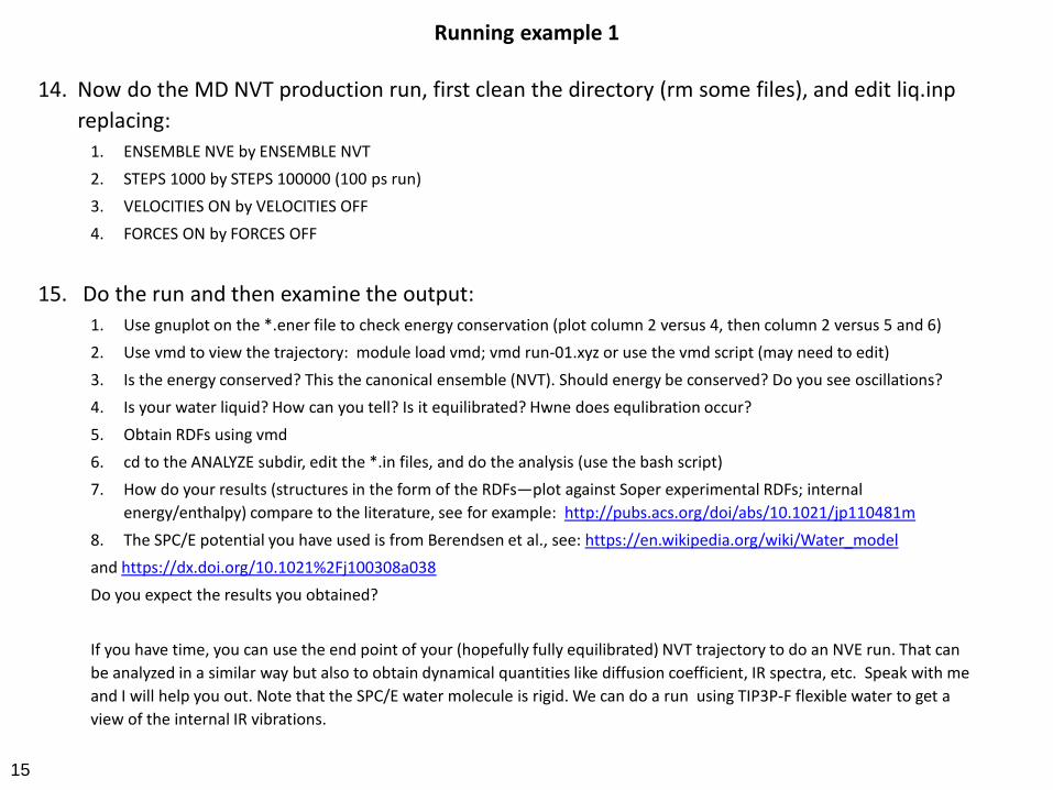
Running example 1

14. Now do the MD NVT production run, first clean the directory (rm some files), and edit liq.inp

replacing:

1. ENSEMBLE NVE by ENSEMBLE NVT

2. STEPS 1000 by STEPS 100000 (100 ps run)

3. VELOCITIES ON by VELOCITIES OFF

4. FORCES ON by FORCES OFF

15. Do the run and then examine the output:

1. Use gnuplot on the *.ener file to check energy conservation (plot column 2 versus 4, then column 2 versus 5 and 6)

2. Use vmd to view the trajectory: module load vmd; vmd run-01.xyz or use the vmd script (may need to edit)

3. Is the energy conserved? This the canonical ensemble (NVT). Should energy be conserved? Do you see oscillations?

4. Is your water liquid? How can you tell? Is it equilibrated? Hwne does equlibration occur?

5. Obtain RDFs using vmd

6. cd to the ANALYZE subdir, edit the *.in files, and do the analysis (use the bash script)

7. How do your results (structures in the form of the RDFs—plot against Soper experimental RDFs; internal

energy/enthalpy) compare to the literature, see for example: http://pubs.acs.org/doi/abs/10.1021/jp110481m

8. The SPC/E potential you have used is from Berendsen et al., see: https://en.wikipedia.org/wiki/Water_model

and https://dx.doi.org/10.1021%2Fj100308a038

Do you expect the results you obtained?

If you have time, you can use the end point of your (hopefully fully equilibrated) NVT trajectory to do an NVE run. That can

be analyzed in a similar way but also to obtain dynamical quantities like diffusion coefficient, IR spectra, etc. Speak with me

and I will help you out. Note that the SPC/E water molecule is rigid. We can do a run using TIP3P-F flexible water to get a

view of the internal IR vibrations.

15

CP2K example 2: Water with DFT @SET BASE_NAME run

@SET ID 01

&GLOBAL

PROJECT ${BASE_NAME}-${ID}

RUN_TYPE MD

&END GLOBAL

&MOTION

&MD

ENSEMBLE NVT

STEPS 20 ! Now you are calculating dft on the fly, it will be much slower

TIMESTEP 0.5

TEMPERATURE 300.0

&THERMOSTAT

TYPE NOSE

REGION MASSIVE

&NOSE

LENGTH 3

YOSHIDA 3

TIMECON [wavenumber_t] 2300

MTS 2

&END NOSE

&END THERMOSTAT

&PRINT ON

&ENERGY

&EACH

MD 1

&END EACH

FILENAME =${BASE_NAME}-${ID}.ener

&END ENERGY

&END PRINT

&END MD

16

&PRINT

&TRAJECTORY ON

&EACH

MD 1

&END EACH

FILENAME =${BASE_NAME}-${ID}.xyz

FORMAT XYZ

&END TRAJECTORY

&VELOCITIES ON

&EACH

MD 1

&END EACH

FILENAME =${BASE_NAME}-${ID}_vel.xyz

FORMAT XYZ

&END VELOCITIES

&FORCES ON

&EACH

MD 1

&END EACH

FILENAME =${BASE_NAME}-${ID}_force.xyz

FORMAT XYZ

&END FORCES

&RESTART ON

&EACH

MD 1

&END EACH

FILENAME =${BASE_NAME}-${ID}.restart

&END RESTART

&END PRINT

&END MOTION

CP2K example 2: Water with DFT (note how sections in blue differ from classical potential example) &FORCE_EVAL

METHOD QS

&DFT

POTENTIAL_FILE_NAME ./GTH_POTENTIALS

BASIS_SET_FILE_NAME ./GTH_BASIS_SETS

! WFN_RESTART_FILE_NAME ./run-01-RESTART.wfn

&MGRID

CUTOFF 280

&END MGRID

&SCF

MAX_SCF 20

EPS_SCF 1.0E-7

SCF_GUESS RESTART

&OUTER_SCF

EPS_SCF 1.0E-7

MAX_SCF 20

&END

&OT T

MINIMIZER DIIS

N_DIIS 7

&END OT

&PRINT

&RESTART ON

&END RESTART

&RESTART_HISTORY OFF

&END RESTART_HISTORY

&END PRINT

&END SCF

&QS

EPS_DEFAULT 1.0E-12

MAP_CONSISTENT

EXTRAPOLATION ASPC

EXTRAPOLATION_ORDER 3

&END QS

17

&XC

&XC_GRID

XC_SMOOTH_RHO NN10

XC_DERIV SPLINE2_SMOOTH

&END XC_GRID

&XC_FUNCTIONAL BLYP

&END XC_FUNCTIONAL

&vdW_POTENTIAL

DISPERSION_FUNCTIONAL PAIR_POTENTIAL

&PAIR_POTENTIAL

TYPE DFTD2

REFERENCE_FUNCTIONAL BLYP

R_CUTOFF 40.0

&END PAIR_POTENTIAL

&END vdW_POTENTIAL

&END XC

&END DFT

&SUBSYS

&CELL

ABC 12.4138 12.4138 12.4138

&END CELL

&COORD

O 1.2025696987709971E+01 1.2412376840360351E+00 1.1100847567157336E+01

H 1.1959096889663195E+01 1.3409373770618183E+00 1.0106406672798471E+01

H 1.1593234139420252E+01 2.0327876480659519E+00 1.1421274324532323E+01

…

O 1.2024298671712041E+01 9.9218625553065536E+00 9.2400384614568534E+00

H 1.2053386790559529E+01 9.6994663967598260E+00 1.0223617621157310E+01

H 1.1277449073604592E+01 9.4150658994176109E+00 8.9496605424081750E+00

&END COORD

&KIND O

BASIS_SET TZV2P-GTH

POTENTIAL GTH-BLYP-q6

&END KIND

&KIND H

BASIS_SET TZV2P-GTH

POTENTIAL GTH-BLYP-q1

&END KIND

&END SUBSYS

&END FORCE_EVAL

!&EXT_RESTART

! RESTART_FILE_NAME ./run-01.restart

!&END EXT_RESTART

Running and analyzing example 2

1. cd $WRKDIR/liq_blypd2_tzv2p_short (this is the input we just went over = Exercise5 for the class)

2. sbatch runit.bash

1. But first: edit if needed the input and script; module load vmd; vmd geometry.xyz or vmd –e liq.vmd to see the starting

geometry

3. While the run is happening, continue the readings or ask questions

4. Examine the output:

1. Use gnuplot on the *.ener file to check energy conservation (plot column 2 versus 4, then column 2 versus 5 and 6)

2. Use vmd to view the trajectory: module load vmd; vmd run-01.xyz or use the vmd script (may need to edit)

3. We only did an extremely short run. Why? Compare timings in the *.ener file to the classical case. How many processor

cores are we using now? How much more costly is Born-Oppenheimer MD with DFT compared to that with a classical

potential 2-body Lennard-Jones plus charges potential?

5. Since this is so costly, you only ran 20 steps to get a feel for DFT-MD. Now you will analyze a pre-

computed long trajectory:

6. cd $WRKDIR/liq_blypd2_tzv2p (this is the identical input but this run went longer)

7. Examine the files as before. Use gnuplot, vmd, etc. You can cd to ANALYZE sub-dir and do analysis.

8. Finally, compare the results of the classical simulation with the DFT one and also with experiment.

You can use gnuplot to plot RDFs obtained from SPC/E and BLYP-D2 and the experimental ones

(Soper files). How do the plots look? What about enthalpy? Put some results together to show

the whole class.

18

Running and analyzing example 3 (formic acid at air-water interface)

1. cd $WRKDIR/water_slab_with_formic_acid_blypd2_dzvp_nve300_short . How does the input file compare to

the one for DFT liquid water? (Hint: use the linux sdiff command: ’sdiff –aw 192 file file2 |less’). What does the

system look like (use: ’vmd geometry.xyz’)? What is the purpose of the vacuum? The constraints?

2. Run it: sbatch runit.bash

3. While the run is happening, continue the readings or ask questions

4. Examine the output

1. Use gnuplot on the *.ener file to check energy conservation (plot column 2 versus 4, then column 2 versus 5 and 6)

2. Use vmd to view the trajectory

3. The formic acid starts to fall. How can we monitor its height above the water surface? (hint ’use grep C position_file > C’,

then use gnuplot) . (Ask me for a gnuplot file to make a good plot.)

4. We only did an extremely short run. Why?

5. Since this is so costly, you only ran 50 steps to get a feel for this problem. Now you will analyze a pre-computed

longer trajectory:

6. cd $WRKDIR/water_slab_with_formic_acid_blypd2_dzvp_nve300 (this is the identical input but this run went

longer, to 10 ps)

7. Examine the files as before. Use gnuplot, vmd (use the scripts and try to understand them), etc. You can cd to

ANALYZE sub-dir and do analysis (first do: ’ssh taito-gpu’, vmd will run faster on gpus). Note that the analyze.x

code called now is slightly different. (You may need to compile it.) Also, vmd is used for calculating RDFs.

8. Is there any chemistry happening? If yes, what are the mechanisms and time scales? (Formic acid is a weak acid

so the deprotonation was not expected. Out of 50 trajectories, I only saw two deprotonate.) Make some nice

vmd snaphots of the Grotthus steps and present to the class. Compare to this Lee et al. paper.

19