Molecular Contamination Modeling with CTSP

Lubos Brieda1,a)

1Particle In Cell Consulting LLC, 21900 Burbank Blvd Ste 300, Woodland Hills, CA 91367

a)Corresponding author: lubos.brieda@particleincell.comURL: https://www.particleincell.com

Abstract. Spacecraft instruments and thermal control surfaces are generally highly sensitive to molecular and particulate contam-ination. Despite best efforts taken during assembly, integration, and test, it is impossible to completely eliminate all sources ofcontaminants. Contamination transport analysis then becomes of critical importance. It can be used to predict the end of life accu-mulation on critical surfaces from prescribed source rates. Conversely, given allowable deposition levels, contamination modelingcan be used to determine the cleanliness requirements to be met prior to launch. This paper describes a recently developed codefor modeling contamination transport. Unlike other tools used by the community, CTSP concurrently traces many simulation par-ticles through small time steps. This allows the code to visualize contaminant partial pressures, and to also include aerodynamic,gravitation, or electrostatic forces. The code is demonstrated by simulating an outgassing characterization test in a bell jar.

INTRODUCTION

Modern spacecraft almost always contain instruments, thermal control surfaces, or mechanical devices that are sus-ceptible to contamination. The term “contamination” refers to the presence of foreign materials that may manifestthemselves either as molecular film, or small, dust-like particulates. Molecular films just few monolayers thick canlead to a significant transmission loss in optical instruments. They also lead to degraded performance of thermalcontrol surfaces[1]. Particulates scatter light and can lead to damage of mechanical or high voltage components[2].Despite best efforts taken during fabrication, integration, and testing, it simply is not possible to completely eliminateall sources of contaminants. Contamination transport modeling then becomes an essential tool in the arsenal of a sys-tems engineer. It can be used to predict the end of life deposition levels given some source rates. Conversely, giventhe allowable end of life deposition, transport modeling can be used to derive the cleanliness requirements to be metprior to launch.

Historically, different methodologies have been applied to molecular and particulate contaminants. Molecularcontaminants, due to their tiny size and mass, are assumed to be unaffected by gravity. They are also assumed toremain neutral. Of interest to the contamination community is the free molecular flow regime in which Knudsennumber Kn � 1. Knudsen number is the ratio of distance traveled by molecules between collisions to a characteristiclength, such as the diameter of the vacuum chamber. In free molecular flow, molecules collide with chamber walls(or spacecraft) more frequently than with each other. Intermolecular collisions can be ignored, and molecules can beassumed to travel in straight lines like photons. This formulation leads to the widespread use of radiation heat transfercodes for contamination analysis[3]. The modeling problem reduces to the task of computing gray body view factorsbetween sensitive surfaces and all outgassing sources. Different methods exist for this calculation including radiosity,which is based on matrix inversion, and Monte Carlo ray tracing.

The primary limitation of the radiation-based approach is that by imposing the straight line trajectories, it be-comes impossible to consider influence of forces on the contaminants. It is well known that molecules exposed to solarradiation undergo photoionization and subsequently backflow to the spacecraft[4]. In the larger particulates, gravita-tional and aerodynamic forces become non-negligible. Historically this required development of specialized codes foreach contributing factor. Some examples include the electrostatic return ESR code[5] and Mastram’s particle modulefor analyzing redistribution in a launch vehicle fairing[6]. A new simulation code CTSP (Contamination TransportSimulation Program) was developed to address these shortcomings. This code is described in this paper. The paperbegins by introducing CTSP and describing the surface model used in the molecular transport analysis. The code is

then demonstrated by simulating an experimental method for determining outgassing rate of a test article placed in avacuum chamber.

CODE OVERVIEW

Particle PushCTSP follows methodology common in Particle in Cell (PIC)[7] or Direct Simulation Monte Carlo (DSMC)[8] codes,and concurrently traces many simulation particles through small ∆t time steps. With the exception of surface inter-action handling, CTSP does not distinguish between molecular and particulate contaminants. Particulates are simplysimulation particles with larger mass and larger cross-sectional surface area. By pushing particles through small timesteps, it is possible to consider velocity change due to action of forces. At each time step, velocities are updated fromNewton’s second law, d~v/dt = ~F/m where ~v is the velocity, m is the particle mass, and ~F is the summation of allforces acting on the particle. CTSP supports gravitational, electrostatic, aerodynamic, and solar pressure forces. Or-bital motion of the parent body can also be defined to model particulate return on orbit crossings. Particle positionis advanced by integrating d~x/dt = ~v using the Leapfrog method. The concurrent push of many particles introducestwo benefits. First, it is now possible to visualize gas bulk properties such as contaminant partial pressure. Secondly,although not yet implemented, the code could be fitted with a DSMC subroutine to consider cases outside the realmof free molecular flow. One application of interest in this transition region is modeling of chamber repressurization.

Geometry and Simulation InputsSimulation geometry is described by a mixed triangular/quadrilateral surface mesh. This mesh is typically generatedfrom a CAD drawing using finite element analysis meshing programs. Surface elements corresponding to the samelogical component need to be collected into groups. The grouping is important since CTSP assigns surface propertiesonly at the group level. The groups are also used to specify particle sources. The code implements multiple injec-tion models applicable to contamination modeling, including outgassing (described below), effusion to model vents,particulate distribution according to the IEST-STD-1246 standard[9], and random coverage by fibers. CTSP does notcontain built-in field solvers, and the appropriate fields needed to compute forces need to be provided by the user.For instance, in order to model particulate fallout in a moving air field, it is necessary to run a CFD analysis to gen-erate a spatial distribution of gas velocity vectors and density scalars. These quantities are then interpolated onto theparticle position. PIC and DSMC codes generally utilize a volume mesh to perform this interpolation. In developingCTSP, decision was made to avoid the need for a volume mesh. In the flow regimes considered by CTSP, there is noappropriate physical parameter usable for sizing the volume cells. In PIC, the cell size is typically based on the localDebye length. In DSMC, the collision mean free path dictates the cell size. But in free molecular flows, the cell sizecould be chosen arbitrarily. Typical CFD solution will contain near-wall region in which the velocity changes rapidly.Interpolating these values onto a too coarse Cartesian grid would result in loss of these fine features. On the otherhand, utilizing the finite element grids from the field solvers would also be impractical, as it would require the codeto track which cell each particle is located for each input grid.

Octree and Surface InteractionsHence, an octree is used to efficiently store the point cloud of field quantities. Prior to each particle push, CTSP firstdefines a control box about the particle’s position. An initially small box is expanded until enough points are retrieved.The located data points ui(~xi) are interpolated onto the particle position ~x using the inverse distance weighting method,u(~x) =

∑Ni=1 wi(~x)ui/

∑Ni=1 wi(~x) with wi(~x) = d(~x, ~xi)−p. Here d is the distance between the points, and p is the

interpolation smoothing factor. An octree is also used to store the surface mesh elements. The starting and finalposition of a particle during a single push is used to define a bounding box. All surface elements located within thebounding box are retrieved from the octree. The code checks for impact by first performing line-plane intersectionsof the line segment traversed by the particle with the plane of the surface element. The intersections are sorted by thedistance from the particle starting point. This step is necessary to account for particles completely traversing through athin surface in a single time step. Next, the intersection point is tested for inclusion within the surface element triangleor quadrangle by looping over all vertices, and forming bisections of vertex angle with a segment to the intersectionpoint. The point is located within the enclosed polyhedral if ∠1 + ∠2 = ∠0 for all vertexes. If intersection is found,

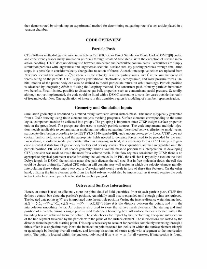
FIGURE 1. Detailed surface interaction model. Only outgassing and surface adsorption/desorption are considered in this work.

the particle is first moved to the surface. The code then calls an intersection handler. This is one areas where CTSPdistinguishes between particulates and molecules. If the impacting particle is a particulate, the intersection handlercomputes the post-impact velocity using a user defined coefficient of restitution, v2 = αrv1. If the resulting velocitymagnitude is less than some threshold, the particle is assumed to become stuck. Its dimensions are then used to updatea histogram of surface particulate distribution. Otherwise, the particle is given a new random velocity away from thesurface and the particle is pushed for the reminder of the time step. Behavior of impacting molecules is based on thesurface residence time, as described below.

Outgassing and DesorptionAs noted in introduction, it is customary to analyze molecular transport by computing gray body view factors be-tween sources and sensitive surfaces. The view factor is then multiplied by the source outgassing rate to obtain thecontribution reaching the target. Besides imposing the straight line trajectory, this approach also ignores the surface-vacuum interface. Molecular outgassing arises from volatile gases trapped inside the material diffusing to the surfaceand desorbing into gas phase. The outgassing rate is not constant. As the amount of trapped material gets depleted,the outgassing rate also goes down. The rate also scales with temperature. It is in fact common to perform a vacuumbakeout of spacecraft components to reduce their initial outgassing rate. The model in CTSP attempts to capture thistemperature dependence. The model is based on the conceptual view shown in Figure 1. All simulation surfaces areassumed to consist of a native substrate containing an arbitrary heterogeneous mixture of trapped gases. At the surfaceis a thin surface layer also composed of an arbitrary combination of molecular species. Initial compositions of the tworegions is specified in the input file for each surface element group as illustrated below:

comp{name:ebox, mat:al, trapped_mass:1e-4, trapped_mats:[0.85*hc1,0.10*water,0.05*n2],surf_h:5e-10, surf_mat:hc1, temp:350}

The amount of mass lost to diffusion is given by[1]

dmdt

= Cm exp(−Ea/RT )tr (1)

where C is a reaction constant, m is the mass, Ea is the material activation energy (typically in kcal/mol), R is thegas constant (kcal K/mole), and T is the temperature (K). For diffusion-limited processes, r = −0.5, although theexample presented in this paper used r = 0 (no time dependence). The reaction constant and activation energy can bedetermined experimentally with the industry standard ASTM-E1559 test[10]. Ea can also be obtained by performinga thermogravimetric analysis (TGA) with a quartz crystal microbalance (QCM). In the absence of either of these datasets, we can estimate activation energy by considering molecular residence time. On a low velocity surface impact, the

molecule temporarily adheres to the surface and establishes thermal equilibrium. The molecule remains attached until,due to random events, it acquires enough energy to escape the electrostatic attraction to the surface. The molecule thenleaves in direction following the cosine law from the surface normal[11]. The time spent on the surface is known asresidence time,

τr = τ0 exp (Ea/RT ) (2)

Here τ0 is the oscillation period of the molecule with typical value ∼ 10−13 s[1]. For most species, the residencetime will be very short except on surfaces below that gas material’s condensation temperature. We can use activationenergies to generate materials characteristic of species commonly encountered in thermal vacuum tests. For instance,molecule with Ea = 12 kcal/mol will have τr of less than 10−5 s on a 350K surface. The residence time increases toover 10,000 s if the surface is cooled to 150K. This value of Ea can thus be used to characterize a generic hydrocarbonthat is driven off at warmer temperatures but sticks to all cold surfaces. A contaminant layer will build up on thesurface as long as the arrival rate exceeds the rate of departure. For deposition thickness less than a monolayer, therate of evaporation is given by first order desorption[11],

dNdt

=1τr

N (3)

Numerical ImplementationWhen a molecule impacts a surface, CTSP computes residence time using equation 2 at the temperature of the im-pacted surface element. If τr ≤ ∆t, the particle is re-emitted. First new velocity magnitude vt is sampled from theMaxwellian speed distribution function at the surface temperature. The particle’s new speed is set to v + αa(vt − v),where αa is the thermal accommodation coefficient. Full accommodations αa = 1 was assumed in the example pre-sented in this paper. The new velocity direction follows the cosine law, which is sampled according to [8]. On theother hand, if τr > ∆t, the particle is adsorbed into the surface layer. Numerically, this involves removing the particlefrom the simulation and incrementing surface count of particle’s material i by the specific weight, ∆Ni = wsp. Thecounts can be related to surface layer thickness by h = N(4/3)πr3/Ael, where r is the molecular radius. Outgassing isimplemented as a source called by the main loop at every time step. The algorithm computes the amount of outgassedmass for each component from equation 1. The mass, converted to number of molecules, is moved to the surfacelayer. The incremental value for each surface element j is scaled by the local area ratio, A j/Atot, where Atot is the totalsurface area of the component. Next, the code loops through all surface elements, and for each computes the amountof mass lost to desorption per equation 3. For cold surfaces, this value will be too small to produce particles. Thesurface layer is depleted according to the number of generated particles. The benefit of this approach is that insteadof utilizing surface sticking coefficients, the impact behavior is determined solely by material properties and surfacetemperature. The overall algorithm can be summarized by the pseudocode below:

load material data (density, molecular radius, TML, ...)load component data (temperature, total mass, cleanliness level, ...)initialize surface data structures

for each timestep:#particle pushfor each particle:

update velocity and positionif surface impact:

compute residence timeif greater than time step:

deposit to surface layerelse:

re-emit following cosine law

#outgassing modelfor each component:

compute outgassing mass lossadd to surface layer

#desorptionfor each surface element:

compute desorption lossinject particles with cosine distributiondeplete surface layer

NUMERICAL EXAMPLE

To demonstrate the code, we consider a commonly encountered engineering task: characterizing the outgassing rateof a test article exposed to vacuum. Figure 2 shows the setup. The test article (a harness) is placed on a platen insidea bell jar. A curved duct connects the bell jar to a vacuum pump. Inside the bell jar is a scavenger plate that can beflooded with cryogenic nitrogen to create a secondary pumping surface. Single quartz crystal microbalance (QCM) isalso placed near the harness. This test corresponds to a “hot-wall” configuration in which the bell jar surface and theplatten are not cold enough to condense the contaminant.

View factor

QCMs indirectly measure mass deposition rate on the exposed crystal. However of interest is the outgassing rate fromthe test hardware. We can start with a mass conservation equation,

ΓhAh − ΓqAq − ΓpAp = 0 (4)

where Γ and A correspond to mass flux and surface area, respectively, and the subscripts h, q, and p stand for hardware,QCM, and pump. The pump term is a placeholder for all other surfaces cold enough to collect the contaminant. If theQCM and pumps are equally cold sinks, Γq = Γp, and the above equation simplifies to ΓhAhkh→q = ΓqAq where

kh→q =Aq

Aq + Ap(5)

is the view factor. In other words, knowing kh→q, we can relate the deposition rate on the QCM to the outgassing rateof the hardware. Although this calculation appears trivial, the difficulty arises from not having a value for Ap, theeffective pump area. Simply considering the cross-sectional area of the pump would ignore pumping inefficienciesand, more importantly, would ignore conductance losses through the duct[11]. Fortunately, we can obtain the pumparea by temporarily introducing a secondary collecting surface of a known area[12]. The scavenger plate in the modelserves this role. We can then write two equations, one without and one with the scavenger plate,

ΓhAh

(Aq

Aq + Ap

)=

(Γq

)1

Aq (6)

ΓhAh

(Aq

Aq + Ap + As

)=

(Γq

)2

Aq (7)

The hardware outgassing term Γh can be eliminated by substitution giving us

Ap

[(Γq

)1−

(Γq

)2

]= Aq

[(Γq

)2−

(Γq

)1

]+ As

(Γq

)2

(8)

Knowing the scavenger plate area and collecting QCM deposition rates without(Γq

)1

and with(Γq

)2

the scavengerplate, we can use the above equation to solve for the effective pump area. This value is then substituted into Equation5 to obtain the hardware outgassing rate.

FIGURE 2. Simulation geometry with the major components identified

RESULTS

The simulation was run for 60,000 time steps at ∆t = 10−4 s. The harness initially contained 0.1 g of a trapped hydro-carbon with Ea = 12 kcal/mol and outgassing rate constant C = 1 s−1. The harness temperature was kept at 350K. Thepump temperature was set to 15K and the QCM crystal was set to 220K. All other surfaces, including the scavenger,were initially at 300K. At time step 30,000, the scavenger was “flooded” by decreasing its temperature to 100K. Thesimulation contained approximately 70,000 particles at steady state and warm scavenger. The count decreased to 4,500once the scavenger was activated due to the increase in total pumping area. We can see the corresponding pressure dropin Figure 3. This Figure plots the partial pressure of the contaminant as well as the surface deposition thickness. Thepartial pressure was computed by interpolating particles onto a three-dimensional Cartesian mesh. As noted earlier,this mesh is used only for visualization and is not used during the particle push. Particle positions and velocities wereinterpolated to compute density and temperature, respectively. The partial pressure was computed from P = nkT . Theinterpolation took place every 5 time steps and was used to update a running average. The volume data was saved toa file every 200 time steps for animation. The cumulative data were cleared after each export. The first plot in Figure3(a) shows the steady-state partial pressure of the contaminant with the warm scavenger. Surface thickness of thedeposited molecular film is also shown. Only the QCM crystal and the pump are cold enough to collect contaminantsand hence are the only surfaces with non-zero deposition thickness. The situation after the scavenger is activated isplotted in Figure 3(b). Chamber pressure decreased by approximately one order of magnitude from 5 × 10−6 Torr to5 × 10−7 Torr. Non-zero deposition is now seen on the scavenger plate.

Pump AreaMass deposited on the QCM crystal versus time step is shown in Figure 4. Over the short duration of the simulation,the hardware outgassing rate is expect to appear constant. This is confirmed by the linear rate of mass increase. Wecan also see a clear difference in slope before and after the scavenger activation at time step 30,000. Microsoft Excel’strendline was used to fit linear curves to the two segment. Of interest is the ratio of slopes. The effective pump area

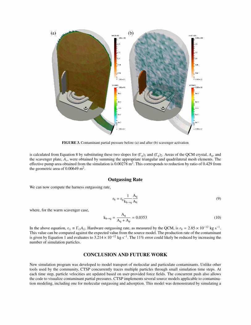
FIGURE 3. Contaminant partial pressure before (a) and after (b) scavenger activation

is calculated from Equation 8 by substituting these two slopes for (Γq)1 and (Γq)2. Areas of the QCM crystal, Aq, andthe scavenger plate, As, were obtained by summing the appropriate triangular and quadrilateral mesh elements. Theeffective pump area obtained from the simulation is 0.00278 m2. This corresponds to reduction by ratio of 0.429 fromthe geometric area of 0.00649 m2.

Outgassing RateWe can now compute the harness outgassing rate,

rh = rq1

kh→q

Aq

Ah(9)

where, for the warm scavenger case,

kh→q =Aq

Aq + Ap= 0.0353 (10)

In the above equation, r() ≡ Γ()A(). Hardware outgassing rate, as measured by the QCM, is rh = 2.85 × 10−12 kg s−1.This value can be compared against the expected value from the source model. The production rate of the contaminantis given by Equation 1 and evaluates to 3.214× 10−12 kg s−1. The 11% error could likely be reduced by increasing thenumber of simulation particles.

CONCLUSION AND FUTURE WORK

New simulation program was developed to model transport of molecular and particulate contaminants. Unlike othertools used by the community, CTSP concurrently traces multiple particles through small simulation time steps. Ateach time step, particle velocities are updated based on user-provided force fields. The concurrent push also allowsthe code to visualize contaminant partial pressures. CTSP implements several source models applicable to contamina-tion modeling, including one for molecular outgassing and adsorption. This model was demonstrated by simulating a

FIGURE 4. Mass collected by the QCM. Difference in rates before and after scavenger plate activation is clearly seen. Computedpump area is also shown.

common engineering task of characterizing the outgassing rate of a test article. A simulation QCM was used to mea-sure deposition rate. Taking into account the effective pump area, it is possible to backtrack the test article outgassingrate from the QCM deposition data. The obtained result agreed within 11% from the expected value. Future workincludes additional code validation, ideally using experimental data. Furthermore, code parallelization is currently inprogress, and preliminary work has been completed on a DSMC module for analyzing the transition region.

REFERENCES

[1] A. Tribble, Fundamentals of Contamination Control (SPIE, 2000).[2] G. E. Galica, B. D. Green, M. T. Boies, O. M. Uy, D. M. Silver, R. C. Benson, R. E. Erlandson, B. E. Wood,

and D. F. Hall, Journal of Spacecraft and Rockets 36 (1999).[3] S. L. O’Dell, D. A. Swartz, N. W. Tice, P. P. Plucinsky, C. E. Grant, H. L. Marshall, A. Vikhlinin, and

A. F. Tennant, “Modeling contamination migration on the chandra x-ray observatory ii,” in SPIE OpticalEngineering+ Applications (International Society for Optics and Photonics, 2013), pp. 88590F–88590F.

[4] A. C. Tribble, B. Boyadjian, J. Davis, J. Haffner, and E. McCullough, “Contamination control engineer-ing design guidelines for the aerospace community,” in SPIE’s 1996 International Symposium on OpticalScience, Engineering, and Instrumentation (International Society for Optics and Photonics, 1996), pp. 4–15.

[5] T. Gordon, Electrostatic return of contaminants, https://see.msfc.nasa.gov/model-esr ().[6] L. Brieda, A. Barrie, D. Hughes, and T. Errigo, “Analysis of particulate contamination during launch of the

mms mission,” in SPIE Optical Engineering+ Applications (International Society for Optics and Photonics,2010), pp. 77940P–77940P.

[7] C. Birdsall and A. Langdon, Plasma physics via computer simulation (Institute of Physics Publishing, 2000).[8] G. Bird, Molecular Gas Dynamics and the Direct Simulation of Gas Flows (Oxford Science Publications,

1994).[9] IEST, Product Cleanliness Levels Applications, Requirements, and Determination (IEST-STD-CC1246D,

2002).[10] ASTM International, Standard Test Method for Contamination Outgassing Characteristics of Spacecraft

Materials (ASTM-E1559, 2009).[11] J. F. O’Hanlon, User’s Guide to Vacuum Technology (Wiley & Sons, 2003).[12] ASTM International, Standard Practice for Spacecraft Hardware Thermal Vacuum Bakeout (ASTM-E2900,

2012).