modified chebyshev-picard iteration methods for

MODIFIED CHEBYSHEV-PICARD ITERATION METHODS FOR SOLUTION

OF INITIAL VALUE AND BOUNDARY VALUE PROBLEMS

A Dissertation

by

XIAOLI BAI

Submitted to the Office of Graduate Studies ofTexas A&M University

in partial fulfillment of the requirements for the degree of

DOCTOR OF PHILOSOPHY

August 2010

Major Subject: Aerospace Engineering


OF INITIAL VALUE AND BOUNDARY VALUE PROBLEMS

A Dissertation

by

XIAOLI BAI

Submitted to the Office of Graduate Studies ofTexas A&M University

in partial fulfillment of the requirements for the degree of

DOCTOR OF PHILOSOPHY

Approved by:

Chair of Committee, John L. JunkinsCommittee Members, David C. Hyland

Srinivas Rao VadaliJohnny HurtadoAniruddha Datta

Head of Department, Dimitris Lagoudas

August 2010

Major Subject: Aerospace Engineering

iii

ABSTRACT

Modified Chebyshev-Picard Iteration Methods for Solution of Initial Value and

Boundary Value Problems. (August 2010)

Xiaoli Bai, B.S., Beijing University of Aeronautics and Astronautics;

M.S., Beijing University of Aeronautics and Astronautics

Chair of Advisory Committee: Dr. John L. Junkins

The solution of initial value problems (IVPs) provides the evolution of dynamic

system state history for given initial conditions. Solving boundary value problems

(BVPs) requires finding the system behavior where elements of the states are defined

at different times. This dissertation presents a unified framework that applies modi-

fied Chebyshev-Picard iteration (MCPI) methods for solving both IVPs and BVPs.

Existing methods for solving IVPs and BVPs have not been very successful in

exploiting parallel computation architectures. One important reason is that most

of the integration methods implemented on parallel machines are only modified ver-

sions of forward integration approaches, which are typically poorly suited for parallel

computation.

The proposed MCPI methods are inherently parallel algorithms. Using Cheby-

shev polynomials, it is straightforward to distribute the computation of force functions

and polynomial coefficients to different processors. Combining Chebyshev polynomi-

als with Picard iteration, MCPI methods iteratively refine estimates of the solutions

until the iteration converges. The developed vector-matrix form makes MCPI meth-

ods computationally efficient.

The power of MCPI methods for solving IVPs is illustrated through a small per-

turbation from the sinusoid motion problem and satellite motion propagation prob-

lems. Compared with a Runge-Kutta 4-5 forward integration method implemented in

iv

MATLAB, MCPI methods generate solutions with better accuracy as well as orders

of magnitude speedups, prior to parallel implementation. Modifying the algorithm

to do double integration for second order systems, and using orthogonal polynomi-

als to approximate position states lead to additional speedups. Finally, introducing

perturbation motions relative to a reference motion results in further speedups.

The advantages of using MCPI methods to solve BVPs are demonstrated by

addressing the classical Lambert’s problem and an optimal trajectory design problem.

MCPI methods generate solutions that satisfy both dynamic equation constraints and

boundary conditions with high accuracy. Although the convergence of MCPI methods

in solving BVPs is not guaranteed, using the proposed nonlinear transformations,

linearization approach, or correction control methods enlarge the convergence domain.

Parallel realization of MCPI methods is implemented using a graphics card that

provides a parallel computation architecture. The benefit from the parallel implemen-

tation is demonstrated using several example problems. Larger speedups are achieved

when either force functions become more complicated or higher order polynomials are

used to approximate the solutions.

v

Dedicated to my parents

for their unconditional love and always being there

vi

ACKNOWLEDGMENTS

First and foremost, I want to thank Dr. John L. Junkins, for his tremendous

guidance and support during my Ph.D. years. His deep understanding of fundamental

knowledge as well as his strong capability to utilize advanced concepts and technology

has greatly influenced and shaped my style of research. His commitment to help stu-

dents and his optimistic attitude toward life have been my source of encouragement.

I have been blessed to take two of his classes on the subject of estimation and celestial

mechanics, which have become my “delightful terminal illness” as he described the

addictive nature of this subject matter. With his remarkable insight into these sub-

jects, his legendary stories drawn from his career experience, and his sense of humor,

to attend his lectures has become a perpetual temptation for me. I know I must be

the object of jealousy from fellow students to be able to meet with him each week

for the past five years . I feel I have been further spoiled to ask for his help when-

ever I needed his insights (even during the weekends or holidays-through Emails),

and almost always I would get an encouraging reply within minutes (even when it

was about my running hobby). Dr. Junkins, you will be a fountain of inspiration

throughout my life!

I would also like to acknowledge the contributions of my committee members,

Drs. David Hyland, Srinivas Vadali, John Hurtado, James Turner, and Aniruddha

Datta. Dr. Hyland’s passion for space exploration inspires me to pursue my dream.

His understanding and assistance to pursue this dream are appreciated beyond words.

It is through Dr. Vadali’s class that I first appreciated the beauty of optimal control.

His ideal scholarship and high quality research drive me to excel in my work. The

opportunity to take two classes from Dr. Hurtado is a precious memory. The passion

he showed in his lectures has deeply influenced and inspired me. Special thanks to Dr.

vii

Turner, who has given me significant support since I came here. I enjoyed the many

research discussions with him in the open atmosphere he provided. I also benefited

a lot from his patience in correcting my English and offering encouragement when I

was frustrated in my research work. Dr. Datta’s modern control class taught me how

to balance the math knowledge and engineering applications, for which I am grateful.

I extend my most sincere thanks to Lisa Willingham for all her help in scheduling

meetings, making travel plans, and getting so much paper work done. Special thanks

to Karen Knabe! Her highly efficient work and her always big smile helped me greatly

during several challenging times. Karen, I can not express how fortunate the graduate

students are to have you work with us, especially us international students! Thank

you very much for all you do!

I wish to thank Dr. Paul Schumacher, who originally recommended that I inves-

tigate parallel-structured integration methods when we first met in a conference last

year. He introduced me to the challenge of the space catalog maintenance problem,

which has been a great source of motivation for this dissertation. I benefited a lot

through his insightful suggestions on what are the key issues and I look forward to

our future collaboration on the space catalog applications. I want to thank Harold

P. Frisch, who helped me significantly when I was learning NDISCOS for multi-body

dynamic system modeling. Harry’s physical understanding of the problems, user-

oriented modeling style, and the passion to build that pretty model for the Stewart

platform in his house when we tried to understand this problem, amazed me and

nurtured my knowledge to do careful system modeling. I would like to thank Dr.

Hans Josef Pesch, who was very generous to discuss with me several optimal control

problems and also send to me several of his papers from Germany! Having solved so

many challenging and diverse optimal control problems for the space-shuttle, aircraft,

carbonate fuel cells, economics, and many others, Dr. Pesch, thank you for offering

viii

many examples as well as encouragement that I can still contribute something to this

rich field, even just a little bit! Exceptional thanks to Daniel P. Scharf. His under-

standing, help, and encouragement on my journey to pursue a dream, have been one

of the most important inspirations for me in the past year. The journey has not been

easy, but it continues motivating me to keep the faith, enjoy the process, and be the

best of myself.

The past five years could not have been so enjoyable without the friendship

with many people including, but not limited to: Daniel Araya, Yun Cai, Jing Cui,

Jeremy Davis, James Doebbler, Zhijun Gong, Troy Henderson, Yongmei Jin, Mrinal

Kumar, Bong Su Koh, Celine Kluzek, Manoranjan Majji, Anshu Narang, Julie Parish,

Carolina Restrepo, Audra Walsh, Laura S. Weber, Lesley Weitz, Whitney Wright, Hui

Yan, Qinliang Zhao. Audra, thank you for inviting me to enjoy the many American

holidays with your family! Every time I hang out with you is so enjoyable and

I am always touched by your stories about the wonderful deaf kids! Jing, thank

you for being my cheer leader since I told you that I wanted to come to the US

to pursue a Ph.D. (about ten years ago). Julie, your help on reading several of my

application essays and your generosity to spend significant time helping me revise this

dissertation, are appreciated more than what I can express. Laura, I feel so blessed

to have you as my friend! The time with you is always relaxing, therapeutic, and

uplifting!

Finally, I offer my gratitude to my family. I wish to thank my elder brother and

sister-in-law, for their belief in me, their support for me to study abroad, and for

taking care of my parents. This dissertation is dedicated to my parents. I am not a

responsible daughter, but they always stand by my side and give me all their love!

Without that, for a girl who was born in a remote Chinese village, life could have

been very different. Thank you my dearest papa and mama, for always letting me

ix

choose the road, which may be less traveled, but the one that I am passionate about.

x

TABLE OF CONTENTS

CHAPTER Page

I INTRODUCTION . . . . . . . . . . . . . . . . . . . . . . . . . . 1

A. Existing Research in Solving IVPs and BVPs using

Methods Related to MCPI Methods . . . . . . . . . . . . . 3

1. Parallel Algorithms for Solving IVPs and BVPs . . . . 3

2. Picard Iteration . . . . . . . . . . . . . . . . . . . . . 4

3. Chebyshev Polynomials . . . . . . . . . . . . . . . . . 5

4. Chebyshev-Picard Methods . . . . . . . . . . . . . . . 7

5. Features of the Modified Chebyshev-Picard Itera-

tion Methods . . . . . . . . . . . . . . . . . . . . . . . 9

B. Application Areas . . . . . . . . . . . . . . . . . . . . . . . 11

1. Orbit Propagation . . . . . . . . . . . . . . . . . . . . 11

2. Lambert’s Problem . . . . . . . . . . . . . . . . . . . . 12

3. Optimal Control Problems . . . . . . . . . . . . . . . 12

II PROBLEM STATEMENT ANDMETHODOLOGYOFMCPI

METHODS . . . . . . . . . . . . . . . . . . . . . . . . . . . . . 14

A. Introduction . . . . . . . . . . . . . . . . . . . . . . . . . . 14

B. Problem Statement of IVPs and BVPs . . . . . . . . . . . 14

C. Modified Chebyshev-Picard Iteration Methods . . . . . . . 15

D. Vector-Matrix Forms of MCPI Methods . . . . . . . . . . . 20

E. Summary . . . . . . . . . . . . . . . . . . . . . . . . . . . 27

III MODIFIED CHEBYSHEV-PICARD ITERATION METH-

ODS FOR SOLUTION OF INITIAL VALUE PROBLEMS . . . 28

A. Introduction . . . . . . . . . . . . . . . . . . . . . . . . . . 28

B. Convergence Analysis of MCPI Methods . . . . . . . . . . 28

C. Piecewise MCPI Methods for Solving IVPs . . . . . . . . . 34

D. Using MCPI Methods to Solve Second Order IVPs with

Only Position Integration . . . . . . . . . . . . . . . . . . . 34

E. Perturbation Motion MCPI Methods . . . . . . . . . . . . 36

F. Numerical Examples . . . . . . . . . . . . . . . . . . . . . 38

1. Small Perturbation from the Sinusoid Motion . . . . . 38

xi

CHAPTER Page

2. Satellite Motion Integration by a Piecewise MCPI

Approach . . . . . . . . . . . . . . . . . . . . . . . . . 46

3. Results of the Position Only MCPI Method . . . . . . 50

4. Zonal Harmonic Perturbation Satellite Motion Prop-

agation Problems . . . . . . . . . . . . . . . . . . . . . 56

G. Parameters Affecting the Performance of MCPI Methods . 59

H. Summary . . . . . . . . . . . . . . . . . . . . . . . . . . . 63

IV MODIFIED CHEBYSHEV-PICARD ITERATION METH-

ODS FOR SOLUTION OF BOUNDARY VALUE PROBLEMS 65

A. Introduction . . . . . . . . . . . . . . . . . . . . . . . . . . 65

B. Three Forms of BVPs for Second Order Systems . . . . . . 65

C. Applying MCPI Methods to a Linear Second Order System 66

1. Solving Final Value Problems . . . . . . . . . . . . . . 67

2. Solving BVPs of the First Kind . . . . . . . . . . . . . 70

3. Solving BVPs of the Second and Third Kind . . . . . 75

D. Applications to Lambert’s Problem . . . . . . . . . . . . . 78

E. An Optimal Control Example: Earth to Apophis Opti-

mal Trajectory Design . . . . . . . . . . . . . . . . . . . . 84

1. Introduction . . . . . . . . . . . . . . . . . . . . . . . 84

2. Frame Definition and Dynamic Equations . . . . . . . 86

3. Optimality Criterion and First Order Conditions . . . 88

4. Solutions from MCPI Methods . . . . . . . . . . . . . 90

5. Solutions from a Chebyshev Pseudospectral Method . 96

F. Summary . . . . . . . . . . . . . . . . . . . . . . . . . . . 101

V DIFFERENT TECHNIQUES TO ENLARGE THE CON-

VERGENCE DOMAIN OF MCPI METHODS . . . . . . . . . . 102

A. Introduction . . . . . . . . . . . . . . . . . . . . . . . . . . 102

B. Aitken’s Process . . . . . . . . . . . . . . . . . . . . . . . . 102

C. The Linearization Approach . . . . . . . . . . . . . . . . . 107

D. Correction Control MCPI Methods . . . . . . . . . . . . . 109

E. Numerical Examples . . . . . . . . . . . . . . . . . . . . . 110

1. Characteristics of Convergence of MCPI Methods

for Solving IVPs and BVPs . . . . . . . . . . . . . . . 110

2. Using the Aitken MCPI Methods to Solve Lam-

bert’s Problem . . . . . . . . . . . . . . . . . . . . . . 116

xii

CHAPTER Page

3. Using the Linearization MCPI Methods to Solve a

Linear Problem . . . . . . . . . . . . . . . . . . . . . . 118

4. Using Correction Control MCPI Methods to Solve

IVPs and BVPs . . . . . . . . . . . . . . . . . . . . . 121

F. Summary . . . . . . . . . . . . . . . . . . . . . . . . . . . 132

VI IMPLEMENTATION OFMCPI METHODS USING GRAPH-

ICS PROCESSING UNITS . . . . . . . . . . . . . . . . . . . . . 133

A. Introduction . . . . . . . . . . . . . . . . . . . . . . . . . . 133

B. NVIDIA Graphics Processing Units . . . . . . . . . . . . . 135

C. CUDA Environment and CUBLAS Toolbox . . . . . . . . 136

D. Graphic Card Testing . . . . . . . . . . . . . . . . . . . . . 138

E. GPU-Accelerated MCPI Methods for Solving the Small

Perturbation from the Sinusoid Motion Problem . . . . . . 141

1. Sequential MCPI and GPU-accelerated MCPI in C . . 141

2. GPU-Accelerated MCPI in C and Sequential MCPI

in MATLAB . . . . . . . . . . . . . . . . . . . . . . . 142

F. GPU-accelerated MCPI Methods for Zonal Harmonic

Perturbation Involved Satellite Motion Propagation Problems143

G. Summary . . . . . . . . . . . . . . . . . . . . . . . . . . . 147

VII CONCLUSIONS . . . . . . . . . . . . . . . . . . . . . . . . . . . 148

REFERENCES . . . . . . . . . . . . . . . . . . . . . . . . . . . . . . . . . . . 152

APPENDIX A . . . . . . . . . . . . . . . . . . . . . . . . . . . . . . . . . . . 161

APPENDIX B . . . . . . . . . . . . . . . . . . . . . . . . . . . . . . . . . . . 163

VITA . . . . . . . . . . . . . . . . . . . . . . . . . . . . . . . . . . . . . . . . 167

xiii

LIST OF TABLES

TABLE Page

I Time comparison of matrix multiplication A×B = C . . . . . . . . 140

II Time comparison of sequential MCPI and GPU-accelerated MCPI

in C . . . . . . . . . . . . . . . . . . . . . . . . . . . . . . . . . . . . 141

III Time comparison of sequential MCPI in MATLAB and GPU-

accelerated MCPI in C . . . . . . . . . . . . . . . . . . . . . . . . . . 142

xiv

LIST OF FIGURES

FIGURE Page

1 Steps of MCPI methods for solving IVPs . . . . . . . . . . . . . . . . 18

2 Steps of MCPI methods for solving BVPs . . . . . . . . . . . . . . . 19

3 Flowchart of the vector-matrix form of the MCPI Approach . . . . . 26

4 Max eigenvalue of Cx . . . . . . . . . . . . . . . . . . . . . . . . . . . 31

5 Max eigenvalue of Cα . . . . . . . . . . . . . . . . . . . . . . . . . . 32

6 Max eigenvalue of CxCα (N:1-100) . . . . . . . . . . . . . . . . . . . 32

7 Max eigenvalue of CxCα(N : 1− 1000) . . . . . . . . . . . . . . . . . 33

8 Integration errors and CPU time comparison (ǫ = 0.01, H = 64π) . . 39

9 Integration errors and CPU time comparison (ǫ = 0.01, H = 128π) . 40





14 Polynomial order for the MCPI method (ǫ = 0.01) . . . . . . . . . . 43

15 Speedup by using the MCPI method(ǫ = 0.01) . . . . . . . . . . . . . 43

16 Polynomial order for the MCPI method (ǫ = 0.001) . . . . . . . . . . 44

17 Speedup by using the MCPI method(ǫ = 0.001) . . . . . . . . . . . . 44

18 Error history of MCPI and ODE45 for ten orbit (two-body problem) 48

19 CPU time of MCPI and ODE45 (two-body problem) . . . . . . . . . 48

xv

FIGURE Page

20 Speedup of MCPI over ODE45 (two-body problem) . . . . . . . . . . 49

21 CPU time of ODE45, MCPI, and position only MCPI (two-body

problem) . . . . . . . . . . . . . . . . . . . . . . . . . . . . . . . . . 50

22 Speedup of position only MCPI over ODE45 (two-body problem) . . 51

23 Speedup of position only MCPI over the original MCPI (two-body

problem) . . . . . . . . . . . . . . . . . . . . . . . . . . . . . . . . . 51

24 Configuration of the three-body motion . . . . . . . . . . . . . . . . 54

25 Relative position errors based on FG solution (three-body motion) . 55

26 Speedup of position only MCPI over ODE45 (three-body motion) . . 55

27 CPU time of different MCPI and ODE45 (two-body motion) . . . . . 57

28 Speedup of different MCPI and ODE45 (two-body motion) . . . . . . 58

29 CPU time comparison (two-body problem) . . . . . . . . . . . . . . . 61

30 Max distance error comparison (two-body problem) . . . . . . . . . . 62

31 Integration errors of y (final value problem) . . . . . . . . . . . . . . 68

32 Integration errors of y (final value problem) . . . . . . . . . . . . . . 69

33 Integration errors of y (y(-1) and y(1)) are known) . . . . . . . . . . 72

34 Integration errors of y (y(-1) and y(1) are known) . . . . . . . . . . . 72

35 Integration errors of y (y(−1) and y(1) are known) . . . . . . . . . . 73

36 Integration errors of y (y(−1) and y(1) are known) . . . . . . . . . . 74

37 Integration errors of y (y(-1) and yd(1) are known) . . . . . . . . . . 76

38 Integration errors of y (y(-1) and yd(1) are known) . . . . . . . . . . 76

39 Integration errors of y (y(1) and yd(-1) are known) . . . . . . . . . . 77

40 Integration errors of y (y(1) and yd(-1) are known) . . . . . . . . . . 77

xvi

FIGURE Page

41 Speedup of MCPI over the fsolve reference solution . . . . . . . . . . 82

42 Speedup of MCPI over a Battin’s reference solution . . . . . . . . . . 82

43 Errors of MCPI and a Battin’s reference solution . . . . . . . . . . . 83

44 Frame, State and Control Definition . . . . . . . . . . . . . . . . . . 86

45 Transfer orbit (Earth to Apophis) . . . . . . . . . . . . . . . . . . . . 92

46 Thrust angle history (Earth to Apophis) . . . . . . . . . . . . . . . . 92

47 Relative errors of the radius (Earth to Apophis) . . . . . . . . . . . . 93

48 Relative errors of the phase angle (Earth to Apophis) . . . . . . . . . 93

49 Relative errors of the radial velocity (Earth to Apophis) . . . . . . . 94

50 Relative errors of the tangential velocity (Earth to Apophis) . . . . . 94

51 Relative errors of the thrust angle (Earth to Apophis) . . . . . . . . 95

52 Relative errors of the radius (pseudospectral) . . . . . . . . . . . . . 98

53 Relative errors of the phase angle (pseudospectral) . . . . . . . . . . 99

54 Relative errors of the radial velocity (pseudospectral) . . . . . . . . . 99

55 Relative errors of the tangential velocity (pseudospectral) . . . . . . 100

56 Relative errors of the thrust angle (pseudospectral) . . . . . . . . . . 100

57 Implement the derived Aitken’s process . . . . . . . . . . . . . . . . 105

58 Convergence history using different transformations . . . . . . . . . . 106

59 Max relative distance error (IVP) . . . . . . . . . . . . . . . . . . . . 111

60 Convergence rate of the max distance error (IVP) . . . . . . . . . . . 112

61 Norm of the corrections (IVP) . . . . . . . . . . . . . . . . . . . . . . 112

62 Correction rate (IVP) . . . . . . . . . . . . . . . . . . . . . . . . . . 113

xvii

FIGURE Page

63 Relative initial velocity error (BVP) . . . . . . . . . . . . . . . . . . 113

64 Convergence rate of the initial velocity error (BVP) . . . . . . . . . . 114

65 Norm of the corrections (BVP) . . . . . . . . . . . . . . . . . . . . . 114

66 Correction rate (BVP) . . . . . . . . . . . . . . . . . . . . . . . . . . 115

67 Iteration number comparison (BVP) . . . . . . . . . . . . . . . . . . 117

68 CPU time comparison (BVP) . . . . . . . . . . . . . . . . . . . . . . 117

69 Error history of the MCPI method (Tf = 5s) . . . . . . . . . . . . . 119

70 Error history of the linearization MCPI method (Tf = 5s) . . . . . . 119

71 Error history of the linearization MCPI method (Tf = 10s) . . . . . . 120

72 Correction history using MCPI . . . . . . . . . . . . . . . . . . . . . 121

73 Relative position errors using MCPI . . . . . . . . . . . . . . . . . . 122

74 Correction history using correction control MCPI . . . . . . . . . . . 122

75 Relative position errors using correction control MCPI . . . . . . . . 123

76 Transfer orbit with time of flight 150 days . . . . . . . . . . . . . . . 124

77 Error of the radius (150 days) . . . . . . . . . . . . . . . . . . . . . . 125

78 Relative error of the phase angle (150 days) . . . . . . . . . . . . . . 125

79 Error of the radial velocity (150 days) . . . . . . . . . . . . . . . . . 126

80 Error of the tangential velocity (T150 days) . . . . . . . . . . . . . . 126

81 Error of the thrust angle (150 days) . . . . . . . . . . . . . . . . . . 127

82 Error of the costate about radius (150 days) . . . . . . . . . . . . . . 127

83 Error of the costate about phase angle (150 days) . . . . . . . . . . . 128

84 Error of the costate about radial velocity (150 days) . . . . . . . . . 128

xviii

FIGURE Page

85 Error of the costate about tangential velocity (150 days) . . . . . . . 129

86 Iteration number comparison (150 days) . . . . . . . . . . . . . . . . 130

87 CPU time comparison (150 days) . . . . . . . . . . . . . . . . . . . . 131

88 Implementation of MCPI methods using CUDA and CUBLAS . . . . 138

89 Computation time of GPU-accelerated MCPI and MATLABMCPI

(N=127) . . . . . . . . . . . . . . . . . . . . . . . . . . . . . . . . . . 144

90 Computation time of GPU-accelerated MCPI and MATLABMCPI

(N=511) . . . . . . . . . . . . . . . . . . . . . . . . . . . . . . . . . . 144

91 Speedup of GPU-accelerated MCPI over MATLAB MCPI (N=127) . 145

92 Speedup of GPU-accelerated MCPI over MATLAB MCPI (N=511) . 145

93 Relative position difference between GPU-accelerated MCPI and

MATLAB MCPI (N=511) . . . . . . . . . . . . . . . . . . . . . . . . 146

94 Chebyshev Polynomials of the first kind . . . . . . . . . . . . . . . . 166

1

CHAPTER I

INTRODUCTION

Improved methods for solving initial value problems (IVPs) and boundary value prob-

lems (BVPs) are of fundamental importance for analyzing and controlling dynamic

systems that are described by ordinary differential equations. IVP solutions generate

trajectories showing how the dynamic system evolves with time with the given initial

conditions; whereas BVP solutions give the system trajectories that satisfy several

constraints defined at different times. Although there already exists a large literature

for solving IVPs and BVPs, there remain several challenges and therefore a need to

improve the current methods and develop new approaches. Among the issues are: (i)

How to significantly reduce the computational burdens; and (ii) How to optimize the

approaches to utilize emerging parallel computing architectures.

This dissertation proposes a modified Chebyshev-Picard Iteration (MCPI) method-

ology to solve IVPs and BVPs. Compared with most existing methods (that are based

on the forward numerical integration methods) to solve IVPs and either the direct

or indirect methods (see definitions in Section 3) to solve BVPs, the proposed MCPI

methods are designed for computational parallelization so they can take advantage

of the rapidly developing parallel technology. Applications of MCPI methods to sev-

eral celestial mechanics problems are explored. The studies show that the proposed

MCPI methods can achieve both computational efficiency and high accuracy, even

prior to parallel implementation. One challenge of the proposed MCPI methods, the

limited convergence domain, is addressed by proposing several techniques that are

shown to enlarge the convergence domain. Using a Graphics Processing Unit (GPU)

The journal model is IEEE Transactions on Automatic Control.

2

architecture, we discuss one parallel implementation of MCPI methods and illustrate

the benefit of using this approach.

The remainder of this chapter is organized as the follows: In Section A, existing

parallel algorithms used to solve IVPs and BVPs are discussed, followed by a discus-

sion of historical literature on using Picard iterations, Chebyshev polynomials, and

Chebyshev-Picard methods for solving IVPs and BVPs. In the context of the exist-

ing Chebyshev-Picard methods, the unique features of the proposed MCPI methods

are then summarized. Section B presents several IVP and BVP application fields to

which the methods developed in this dissertation are applicable.

The remainder of this dissertation is arranged as follows: Chapter II introduces

formal statements of IVPs and BVPs that are the focus of this dissertation and

develops MCPI methods that can be modified to solve both IVPs and BVPs. A

vector-matrix form of MCPI methods is then presented. The related fundamentals

of the classical Picard iteration and Chebyshev polynomials are summarized in Ap-

pendix A and Appendix B, for the readers’ convenient reference. Chapter III focuses

on applying the MCPI methodology to solve IVPs. A piecewise approach to solve

IVPs over an arbitrary time interval is discussed. Several modifications that improve

the performance of MCPI methods for solving IVPs are presented. Simulation re-

sults of the applications for a small perturbation problem, a two-body problem, and

a three-body problem are presented and compared with a conventional Runge-Kutta

4-5 integration method. Chapter IV focuses on using the MCPI methodology to solve

BVPs. The strategy for solving different types of BVPs is illustrated using a linear

second order system. The applications of the MCPI approach to the classical Lam-

bert’s two-point boundary value problem and an optimal trajectory design problem

are also discussed in detail. Different techniques for enlarging the MCPI convergence

domain are presented in Chapter V. The benefits of using these techniques are shown

3

through several examples. Chapter VI presents a parallel implementation of MCPI

methods using a GPU card. In Chapter VII, conclusions and directions for future

extension are discussed.

A. Existing Research in Solving IVPs and BVPs using Methods Related to MCPI

Methods

1. Parallel Algorithms for Solving IVPs and BVPs

Compared with the significant achievement of using parallel computation techniques

in other scientific computation fields, research on developing parallel algorithms to

solve IVPs is advancing at a slower speed. This is because most of the current pop-

ular numerical integration methods do not have properties that lend themselves to

parallel computation [1]. Franklin [2] compared three approaches to parallelize the

existing forward integration methods: a parallel block implicit method, segmenting

the equations to separate parts which can be solved using various processes, and revis-

ing the forward integration methods to a parallel-corrector form which was designed

by Miranker and Liniger [3]. As many existing methodologies are limited to small

scale problems (the number of the processors is small), Gear derived parallel algo-

rithms targeted on large scale problems, but Gear’s algorithms are only applicable

for some special cases [1]. Although no illustrations were provided, Gear speculated

that realizing a parallel structure for quadrature and function evaluation should be

emphasized when designing more powerful methods. Gear’s remarks provide a partial

motivation and a qualitative context for this dissertation.

There has also been significant interest in using the parallel architectures for

numerical optimization. Much of the recent progress can be categorized as either

devising parallel linear algebra software and algorithms or developing new parallel

4

strategies in global optimization [4]. In the optimal control field, Travassos [5] sug-

gested using Miranker and Liniger’s algorithms for parallel integration [3]. He also

compared two parallel algorithms for function minimization, and discussed using a

parallel shooting method to solve for the unknown initial costates. The level of par-

allelism of his approach is n(2N − 1), where n is the dimension of the states and N

is the number of subintervals used in the parallel shooting. Betts and Huffman [6]

broke the overall trajectory into phases to parallelize the trajectory optimization al-

gorithms. The sparse Jacobian matrix resulting from the multiple shooting method

was solved using sparse finite differences by parallel computation. They implemented

the algorithm on BBN GP100 (Butterfly) parallel processor for four obit transfer

problems and the speedups were in the range of 1.9 to 9.9. However, the results

showed that their proposed parallel approach was not always faster than the serial

direct approach, and the authors suggested this is because additional variables and

constraints were introduced by the way they parallelized their problems.

2. Picard Iteration

Picard iteration is a successive solution approximation technique that is often used

to prove the existence and uniqueness of the solutions to IVPs (detailed description

in Appendix A). Although this approach is most often connected with the names of

Charles Emile Picard, Ernst Lindelof, Rudolph Lipschitz and Augustin Cauchy, it

was first published by the French mathematician Joseph Liouville in 1838 for solving

second order homogeneous linear equations. About fifty years later, Picard devel-

oped a much more generalized form, which placed the concept on a more rigorous

mathematical foundation, and used this approach to solve boundary value problems

described by second order ordinary differential equations [7]. The type of the bound-

ary value problems he considered belongs to BVPs of the first kind (see definition in

5

Chapter IV). Picard developed a theoretical condition for the length of the intervals

under which Picard iteration is guaranteed to converge. Including Picard himself,

many authors have worked on improving these conditions [8, 9, 10, 11, 12]; gener-

ally these developments have sought to make Picard’s original convergence conditions

sharper and less conservative. However, these conditions, even after several improve-

ments, still only provide a conservative estimate on the region of the convergence;

the “best possible” interval where Picard iteration converges, for a general problem,

is not yet known. Also, there are a number of counterexamples in which Picard iter-

ation is guaranteed not to converge, even if the starting function is arbitrarily close

to the real solution [13, 14]. For multiple-point BVPs of the first kind, Urabe proved

the sufficient conditions under which the approximate solution ensures the existence

of the exact solution and presented an approach to calculate the error boundary for

the approximation [15]. Coles and Sherman [12] are among the few who studied the

convergence domain of Picard iteration for BVPs of the second and third kind (see

definition in Chapter IV). Shridharana and Agarwal discussed how to construct a

Picard-iteration-like sequence that will converge to the exact solutions [16]. How-

ever, except for some simple cases, their constructive theory is difficult to implement.

Parker and Sochacki have studied the use of Picard iteration to generate solutions of

IVPs in the form of Taylor series [17], however, convergence of this approach is not

generally attractive.

3. Chebyshev Polynomials

Chebyshev polynomials are a complete set of orthogonal polynomials that are very

important for function approximation (description in Appendix B). If the zeros of

Chebyshev polynomials are used as the nodes for polynomial interpolations, the re-

sulting approximating polynomial minimizes the Runge’s phenomenon and provides

6

the best approximation under the minimax norm [18]. Furthermore, for this set of

nodes, the Chebyshev polynomials are orthogonal with a unit weight function.

Many researchers have contributed to the research on using Chebyshev polynomi-

als to solve IVPs and BVPs [18, 19, 20, 21, 22, 23, 24, 25]. Urabe has made several im-

portant theoretical contributions. Using Newton’s method and successive Galerkin’s

approximation, Urabe proved that the existence of an isolated periodic solution lying

in the interior of the region where the differential equation is defined always implies the

existence of Galerkin approximations of orders sufficiently high [23]. Furthermore, he

showed that if there exists a Galerkin approximation of sufficiently high order, under

some smoothness conditions, an exact solution exists and the approximation error can

be determined. Urabe also discussed a numerical computation approach for periodic

nonlinear systems using the Galerkin approximations [24]. Recently Chen presented

the error bounds of the truncation errors when the two-variable Chebyshev series ex-

pansions are used to approximate the solutions of IVPs [25]. Urabe has also studied

the use of Chebyshev polynomials to solve for the numerical solution of BVPs of the

first kind [26]. He proved that if an isolated solution exists for multi-point BVPs,

there are always Chebyshev approximate solutions that can be as accurate as de-

sired. Furthermore, he showed that under some conditions, the obtained Chebyshev

approximate solution insures the existence of the exact solution, and the error bound

can be obtained. However, practical numerical methods for finding the Chebyshev

coefficients using this approach are difficult to design (this assessment agrees with the

discussion by Vlassenbroeck and Dooren [27]).

There have also been studies of using Chebyshev polynomials to solve optimal

control problems, most of which belong to the set of direct methods. Vlassenbroeck

and Dooren proposed using Chebyshev polynomials to approximate the state and con-

trol variables [27]. By approximating the performance function, dynamic equations,

7

and constraints, the original nonlinear optimal control problem is transformed into an

algebraic equation system for the Chebyshev coefficients that are solved with nonlin-

ear programming methods. Similar ideas have been used in other papers [28, 29], with

the major differences of how the performance function and constraints are enforced.

4. Chebyshev-Picard Methods

Except for some special cases, it is usually difficult to use the classical Picard iter-

ation method for solving IVPs and BVPs, because the integrals are not analytically

tractable. Clenshaw and Norton [30] first proposed to solve IVPs and BVPs us-

ing both Picard iteration and Chebyshev polynomials (Chebyshev-Picard methods).

They approximated the trajectory and the integrand by the same orthogonal ba-

sis functions (discrete Chebyshev polynomials) and integrated the basis functions

term-by-term to establish a recursive trajectory approximation technique. Feagin ap-

plied the technique to several BVPs of the first kind [31]. Shave [32] studied using

Chebyshev-Picard methods for orbit propagation and estimation problems based on

the assumption of a single instruction, multiple data (SIMD) parallel architecture.

He achieved high accuracy solutions for satellite motion propagation problems and

also examined the potential time performance improvement that can be achieved by

parallel implementation of Chebyshev-Picard methods. Recently, Sinha and Butcher

developed a method that uses Picard iteration and shifted Chebyshev polynomials

to symbolically solve for the approximate solutions of the state transition matrix for

linear time-periodic dynamic systems [33]. In addition to the work by Shave [32], the

parallel nature of the Chebyshev-Picard methods has also been addressed by Feagin

and Fukushima. Feagin [34] presented a vector-matrix form of the Chebyshev-Picard

method that is closely related to MCPI methods we propose in this dissertation. How-

ever, Feagin only applied the vector-matrix form of the Chebyshev-Picard methods

8

to solve IVPs. The capability to solve both IVPs and BVPs using this vector-matrix

form was not discussed and he also did not provide any practical implementation

or experimental results for solving either IVPs or BVPs. Fukushima implemented a

Chebyshev-Picard algorithm on a vector computer [35]. However, for one example

problem, the vector code was shown to be slower than the scalar code and the author

suggested that this was because his approach could not be vectorized efficiently and

the compilation put more additional overhead.

The issue of limited convergence domain for Chebyshev-Picard methods has been

widely recognized since the beginning of this avenue of research, whereas the problem

has not been finally solved up to today. In their pioneering paper, Clenshaw and

Norton correctly concluded that the convergence for the proposed Chebyshev-Picard

method, which is quite good in many problems, is not generally guaranteed. They sug-

gested additional research to design more powerful methods for two-point BVPs [30].

Later, Norton proposed using what he called “Newton iteration formula” to solve

the nonlinear ordinary differential equations in Chebyshev series [22]. The formulas

for scalar ordinary differential equation are derived. He also discussed using iterative

solutions to solve for the Chebyshev coefficients associated with the resulting linear

equations for some special cases. Wright compared a Picard method, a linearization

method, and some Taylor-series-based techniques for solving the problems associ-

ated with the Chebyshev collocation methods [21]. What he called the linearization

method is essentially the same as the Newton iteration formula proposed by Norton.

Wright showed several examples where the linearization method found the solutions

but the classical Chebyshev-Picard method diverged. In his dissertation, Feagin ex-

tended the Newton iteration formula in Norton’s paper to vector cases and derived

formulas for second order differential equations [31]. Realizing the difficulty of solving

the resulting linear equations for high dimensional problems using the linearization

9

approach, Feagin discussed two methods for improving the direct inversion approach

used by Norton: one is to solve the linear equations using the iterative method pro-

posed by Scraton [20]; the other is to use the successive over-relaxation method [36],

which he showed to be the most efficient.

5. Features of the Modified Chebyshev-Picard Iteration Methods

Motivated by the above research, this dissertation introduces a family of modified

Chebyshev-Picard iteration (MCPI) methods. The proposed MCPI methods, devel-

oped in subsequent chapters, have following four unique features:

• This is the first time that a unified vector-matrix form of Chebyshev-Picard

methods is developed and proven to be applicable to solve both IVPs and BVPs.

• This is the first time that the power of Chebyshev-Picard methods for solving

both IVPs and BVPs has been shown through highly accurate and efficient

solution of several important celestial mechanics problems (even prior to parallel

implementation).

• Several new techniques are proposed in this dissertation that aim to either im-

prove the accuracy performance or enlarge the convergence domain for Chebyshev-

Picard methods. This is the first time that the perturbation motion MCPI

methods are proposed and also shown to improve the performance. The con-

cept of the correction control in Picard iterations is novel. Unlike other existing

techniques to enlarge the convergence domain, this method does not encounter

the curse of dimensionality difficulties when solving high dimensional problems

or when high order polynomials are required to approximate the solutions.

• This is the first time that Chebyshev-Picard methods have been implemented

10

on a graphics card to obtain a parallel implementation. The speedup achieved

from the parallel implementation is the largest that has ever been reported.

We point out that this dissertation has a strong connection with Feagin’s work [31, 34].

In his dissertation, Feagin proposed to combine Chebyshev polynomials with either

Picard iterations or quasilinearization to solve two-point BVPs for spacecraft trajec-

tory design. He also recommended the utilization of Aitken’s process to enlarge the

convergence domain as we do in this dissertation. In the appendix of his dissertation,

Feagin derived a vector-matrix form of Chebyshev-Picard methods for solving IVPs,

which is very similar to the vector-matrix form of MCPI methods we introduce in

Chapter II. However, the differences of this dissertation from the work of Feagin are

significant. In addition to the four distinguishing features we summarized earlier,

we emphasize the following five differences between Feagin’s work and the results

documented in this dissertation:

• The vector-matrix form of MCPI methods we propose is different from the form

Feagin derived. The differences are pointed out in detail in Chapter II.

• The applicability of the vector-matrix form of MCPI methods for solving BVPs

was neither discussed nor used by Feagin.

• Feagin focused on solving the BVPs of the first type (see definition in Chap-

ter IV), whereas we discuss using MCPI methods to solve more general BVPs.

• Feagin did not show any example about using the Chebyshev-Picard method

for solving IVPs.

• Feagin did consider in his dissertation an optimal control problem, however, in

lieu of applying a Picard iteration, he instead used a quasilinearization approach.

11

In this dissertation we discuss using MCPI methods to solve general family of

optimal control problems and we prove the practical merit of this approach.

We mention that the above differences are pointed out for clarity in understanding

the context of this dissertation’s contribution, and certainly in no way minimize the

pioneering and important contributions made by Feagin, whose work proceeded the

present work by almost four decades!

B. Application Areas

We will study the following IVP and BVP applications that are very important in

the celestial mechanism fields.

1. Orbit Propagation

Since the launch of the first satellite (Sputnik 1) in 1957, it has been necessary to

maintain and frequently update database of satellite orbits. This endeavor is referred

to maintaining the space catalog. The ability to propagate satellite motion quickly

and accurately is one of the major factors that affect the completeness, accuracy, and

cost of the database [37], especially as the number of objects in the catalog exceeds

100, 000. The analytic predicator methods, while very efficient, can not meet require-

ments for the task such as collision avoidance and satellite acquisition. Therefore

numerical integration of the satellite motion with even more accurate and compli-

cated perturbation force models has become necessary [38]. The most widely accepted

integrator is an 8th-order multi-step predictor-corrector method known as the Gauss-

Jackson method [38, 39, 40]. However, this choice of integrator does not allow the

SIMD computer to run very efficiently [39]. With the current goal to model around

150, 000 satellites within the next 8 to 10 years with a degree and order 36 × 36 or

12

higher gravity model and a realistic atmospheric density model, and a requirement to

estimate each of these orbits in near-real-time as observations become available, the

extensive force calculation has become a processing bottleneck. Even with the antic-

ipated speedup from Moore’s Law, a true parallel algorithm has become necessary.1

2. Lambert’s Problem

Lambert’s problem is the classical two-point BVP of celestial mechanics that was

first stated and solved by Johann Heinrich Lambert in 1761 [41]. Given two positions

at an initial time and a prescribed final time, Lambert’s problem is to solve for an

initial velocity, using which the generated orbit, connects the two known positions

with the prescribed time of flight. For general perturbed motion, the generalized

Lambert’s problem remains a challenging nonlinear problem that must be frequently

solved today for orbit transfer. Battin developed an elegant, now classical approach

to solve the classical Lambert’s problem [41]. However, his method only works for the

cases that no perturbations to the inverse-square gravity field exist. Numerical iter-

ation techniques such as shooting methods [42] are the most frequently used current

approach to solve the more general perturbed orbit transfer problems.

3. Optimal Control Problems

Given a performance function, a set of ordinary differential equations describing the

dynamic system, and various system constraints, an optimal control design algorithm

solves for the control input that drives the system to execute an optimal trajectory to

minimize or maximize the performance function and satisfy the constraints. The two

most popular sets of computational techniques for solving optimal control problems

1Communication with Dr. Paul W. Schumacher from HSAI-SSA, Air Force Re-search Laboratory

13

are direct shooting and indirect shooting[43] methods. Direct methods introduce a

parametric representation of the control variables (and frequently the state variables

as well), and then use nonlinear programming optimizers to solve the resulting nonlin-

ear parameter optimization problems (a so-called nonlinear programming problem).

With the increasing power of these optimizers, direct approaches can obtain sub-

optimal solutions often more easily than indirect approaches. However, the accuracy

and optimality of the returned control policy for the original continuous system are

not guaranteed. Indirect approaches are based on calculus of variations without pa-

rameterization of state and control variables. Necessary conditions are derived from

Pontryagin’s Principle[44]. A simple shooting or multiple shooting method is usually

used to solve the resulting two-point value problem, with the goal being to find the

unknown initial states and co-states. The solutions obtained from the indirect ap-

proaches assure local optimality and accuracy. However, solving the resulting BVPs

is challenging because the solutions can be very sensitive to the initial guess, and lo-

cal convergence to solutions that satisfy the necessary conditions does not guarantee

global optimality.

Through Pontryagin’s Principle, we consider the optimal control of continuous

systems as a special type of BVPs in this dissertation. We introduce MCPI methods

to solve the state and co-state differential equations, and boundary conditions that

are the necessary conditions for optimality.

14

CHAPTER II

PROBLEM STATEMENT AND METHODOLOGY OF MCPI METHODS

A. Introduction

Formal statements of IVPs and BVPs that are studied in this dissertation are pre-

sented in this chapter. The MCPI methodology is discussed and its vector-matrix

forms to solve IVPs and BVPs are developed. The formulations presented in this

chapter provide the bases for the later chapters to solve IVPs, BVPs, and optimal

control problems.

B. Problem Statement of IVPs and BVPs

The systems we consider in this dissertation are described by ordinary differential

equations (ODEs), for which the independent variable is denoted by the time t and

the vector of dependent variables is represented by x, whose elements include all the

states of the dynamic system. Here we assume higher order ODEs have already been

transformed to their first order forms.

An IVP seeks the solution of x(t) that satisfies the given ODE

dx(t)

dt= f (t,x(t)), t ∈ [a, b] (2.1)

and the given initial condition x(t = a) = x0, where t = a is the initial time and

t = b is the final time. The conditions for the existence and uniqueness of the IVP

solution are the same as the conditions for the classical Picard iterations to converge

(presented in Appendix A).

Although general BVPs can have interior constraint conditions on x at any time

in the interval of [a, b], we focus on two-point BVPs in this dissertation. In this case,

15

a BVP seeks the solution for x(t) that satisfies the given ODE in Eq. 2.1 and the

boundary conditions for x, some of which are defined at the initial time and others

are defined at the final time.

C. Modified Chebyshev-Picard Iteration Methods

We use a scalar case example to illustrate the procedure to solve IVPs using MCPI

methods. Consider a differential equation with an initial condition x(t = a) = x0

dx

dt= f(t, x), t ∈ [a, b] (2.2)

The first step of MCPI methods is to transform the generic independent variable

t to a new variable τ , which is defined on the valid range −1 ≤ τ ≤ 1 of Chebyshev

polynomials through

t =b− a

2τ +

b+ a

2(2.3)

After the substitution, Eq. (2.2) is transformed to a new form as

dx

dτ=

b− a

2f(

b− a

2τ +

b+ a

2, x) ≡ g(τ, x) (2.4)

The Chebyshev polynomial of degree k is denoted by Tk and the (N +1) discrete

nodes that are used to approximate the states are the Chebyshev-Gauss-Lobatto

(CGL) nodes, which are calculated from

τj = cos(jπ/N), j = 0, 1, · · · , N (2.5)

To start the iteration, an initial guess of the solution x0(τ) is required. Assume

the force function appearing on the right hand side of Eq. 2.4 is approximated by a

16

N th order Chebyshev polynomial

dx

dτ= g(τ, x0) ≈

k=N∑

k=0

′FkTk(τ) (2.6)

Using the discrete orthogonality property of Chebyshev polynomials, the coefficients

F0, F1, · · · , FN are calculated immediately from

Fk =2

NΣN

j=0′′g(τj, x

0(τj))Tk(τj) (2.7)

Notice each coefficient Fk is obtained through the summation of (N +1) independent

terms, each of which is the multiplication of the force function g and the Chebyshev

polynomials Tk evaluated at the CGL point τj . Furthermore, all the coefficients

F0, F1, · · · , FN are independent of each other, and can therefore be computed in

parallel processors. Also, for problems where calculating the force function g is time

consuming, significant time performance improvement can be achieved by parallel

computation of g on different processors.

The solution at the next step is assumed as x1(τ) =∑k=N

k=0′βkTk(τ), and the

Picard method provides the iteration form

x1(τ) = x0 +

∫ τ

−1

g(s, x0(s))ds (2.8)

Using the integration properties of Chebyshev polynomials (see Appendix B), using

Eq. 2.6 in Eq. 2.8, one obtains

1

2β0T0(τ) + β1T1(τ) + β2T2(τ) + · · ·βNTN(τ)

= x(−1) +

∫ τ

−1

(

1

2F0T0(s) + F1T1(s) · · ·+ FNTN(s)

)

ds

= c+1

2F0T1(τ) +

1

4F1T2(τ) +

1

2F2

[

1

3T3(τ)− T1(τ)

]

· · ·

+1

2FN

[

1

N + 1TN+1(τ)−

1

N − 1TN−1(τ)

]

(2.9)

17

where c is some constant to be defined according to the given constraints.

For the IVP with the given initial condition x(t = a) = x0, equating the first to

N th order coefficients of the Chebyshev polynomials on the left side and on the right

side of Eq. 2.9 leads to the following formulations to obtain the coefficients

βr =1

2r(Fk−1 − Fk+1), r = 1, 2, · · · , N − 1 (2.10)

βN =FN−1

2N(2.11)

The initial condition leads to the solution for the zero order coefficient, given by

β0 = 2x0 + 2Σk=Nk=1 (−1)k+1βk (2.12)

For two-point BVPs, both the zero and first order coefficients should be calcu-

lated to satisfy the boundary conditions x(t = a) = x0 and x(t = b) = xf , leading to

the update equations for the state approximation coefficients as

βr =1

2r(Fk−1 − Fk+1), r = 2, 3, · · · , N − 1 (2.13)

βN =FN−1

2N(2.14)

β0 = x0 + xf − 2(β2 + β4 + β6 + · · · ) (2.15)

β1 =(xf − x0)

2− (β3 + β5 + β7 + · · · ) (2.16)

The updated coefficients are used to calculate the new trajectory approximation for

the next step. In this way, the solutions are iteratively improved until some accuracy

requirements are satisfied. To account for the nonlinearity issues, the stopping cri-

terion we choose is to require both the difference between the solutions xi and xi−1

and the difference between the solutions xi and xi+1 are less than some tolerance.

Figure 1 shows the steps of MCPI methods for solving IVPs and Fig. 2 shows the

steps of MCPI methods for solving BVPs. Notice when solving BVPs, the MCPI

18

algorithm differs significantly from usual shooting methods: there is no local Tay-

lor series approximations, gradient computations, or matrix inversions. Furthermore,

as a consequence of using an accurate Chebyshev approximation of the integrand on

each iteration, the integration of the Chebyshev solutions is accomplished analytically

when the coefficients are updated.

Starting Guess

Equation Normalization

Iterate

Solution Update

Integrand Approx

Fig. 1. Steps of MCPI methods for solving IVPs

19

Starting Guess

Equation Normalization

Iterate

Solution Update

Integrand Approx

Fig. 2. Steps of MCPI methods for solving BVPs

20

D. Vector-Matrix Forms of MCPI Methods

Instead of term by term to solve for the state value at the (N + 1) CGL nodes, the

(N + 1) Chebyshev coefficients, and the updated (N + 1) Chebyshev coefficients, we

introduce a compact vector-matrix approach to implement MCPI methods. In this

way, we not only solve for the state values and Chebyshev coefficients in a vector

form, but also has a compact formulation to update the coefficients through Picard

iterations. We find that a similar idea has been published by Feagin and Nacozy[34].

There are three major differences between the formulations in their paper and our

derivations. We will point out these differences along the way we derive for the

vector-matrix form of MCPI methods.

The zero to N th order coefficients of the Chebyshev polynomial to approximate

the solution x(τ) are defined in a vector form as

~α = [α0, α1, · · · , αN ]T (2.17)

The solution of x evaluated at the CGL nodes is represented by a vector as

~x = [x(τ0), x(τ1), · · · , x(τN )]T (2.18)

Similar as Eq. 2.6, the solution of x can be calculated from its Chebyshev coefficients

21

through

~x =

12α0T0(τ0) + α1T1(τ0) + · · ·+ αNTN(τ0)

12α0T0(τ1) + α1T1(τ1) + · · ·+ αNTN(τ1)

...

12α0T0(τN ) + α1T1(τN ) + · · ·+ αNTN (τN)

=

T0(τ0) T1(τ0) · · · TN(τ0)

T0(τ1) T1(τ1) · · · TN(τ1)

......

......

T0(τN ) T1(τN ) · · · TN(τN )

12

0 0 0

0 1 0 0

0 0. . . 0

0 0 0 1

α0

α1

...

αN

≡ TW~α

≡ Cx~α (2.19)

with the definition

Cx ≡ TW (2.20)

T =

T0(τ0) T1(τ0) · · · TN(τ0)

T0(τ1) T1(τ1) · · · TN(τ1)

......

......

T0(τN) T1(τN) · · · TN(τN )

(2.21)

and the diagonal matrix W is defined as

W = diag([1

2, 1, 1, · · · , 1, 1]) (2.22)

Notice the last diagonal term in Eq. 2.22 is one since we are using the discrete least-

squares fit (see Appendix B). Although Feagin and Nacozy[34] did not say explicitly

the reason for their formula to have the last term as 12, that is required for exact inter-

polation where the function f(x, t) fits exactly at the interpolation nodes. The most

important reason we choose the least-square fit approach is because this approach

implicitly provides an error bound while for the interpolation approach, this bound

22

will be difficult to determine.

The force function is evaluated at the CGL nodes and defined in a vector form

as

~g = [g(τ0), g(τ1), · · · , g(τN)]T (2.23)

The zero to N th order coefficients of the Chebyshev polynomials for function g are

defined as

~F = [F0, F1, · · · , FN ]T (2.24)

Consistently with Eq. 2.7, these coefficients are calculated from

~F =

1Ng(τ0)T0(τ0) +

2Ng(τ1)T0(τ1) + · · ·+ 1

Ng(τN)T0(τN )

1Ng(τ0)T1(τ0) +

2Ng(τ1)T1(τ1) + · · ·+ 1

Ng(τN)T1(τN )

...

1Ng(τ0)TN(τ0) +

2Ng(τ1)TN (τ1) + · · ·+ 1

Ng(τN)TN(τN)

=

T0(τ0) T0(τ1) · · · T0(τN )

T1(τ0) T1(τ1) · · · T1(τN )

......

......

TN(τ0) TN(τ1) · · · TN(τN )

1N

0 0 0

0 2N

0 0

0 0. . . 0

0 0 0 1N

F0

F1

...

FN

≡ T TV ~g

= TV ~g (2.25)

where the property that T T = T has been utilized. And the diagonal matrix V is

defined as

V = diag([1

N,2

N,2

N, · · · , 2

N,1

N]) (2.26)

The zero to N th order coefficients of the Chebyshev polynomials to approximate

23

the updated solution of x(τ) are defined as

~β = [β0, β1, · · · , βN ]T (2.27)

The formulations from Eqs. (2.10) to (2.12) for updating the coefficients correspond

24

to a vector-matrix form as

~β =

2x0 + 2(β1 − β2 + β3 + · · ·+ (−1)N+1βN)

12(F0 − F2)

12×2

(F1 − F3)

...

12×r

(Fr−1 − Fr+1)

...

FN−1

2N

=

2x0

0

0

...

0

0

+

1 0 0 0 0

0 12

0 0 0

0 0 14

0 0

0 0 0. . . 0

0 0 0 12×r

0

0 0 0. . . 0

0 0 0 0 12N

1 −12

−23

14

− 215

· · · (−1)N+1 1N−1

1 0 −1 0 0 · · · 0

0 1 0 −1 0 · · · 0

......

......

......

...

0 0 0 · · · 1 0 −1

0 0 0 0 · · · 1 0

F0

F1

F2

F3

...

FN−1

FN

= ~χ0 +RS ~F

which can be further written as

~β = ~χ0 +RSTV ~g = ~χ0 + Cα~g (2.28)

25

as we define

RSTV ≡ Cα (2.29)

~χ0 = [2x0, 0, 0, · · · , 0]T (2.30)

R = diag([1,1

2,1

4, · · · , 1

2(N − 1),1

2N]) (2.31)

S =

1 −12

−23

14

− 215

· · · (−1)N+1 1N−1

1 0 −1 0 0 · · · 0

0 1 0 −1 0 · · · 0

......

......

......

...

0 0 0 · · · 1 0 −1

0 0 0 0 · · · 1 0

(2.32)

The first row of matrix S is obtained as we represent β1 to βN in terms of F0 to FN .

The rth(r = 2, 3, · · · , N − 1) column of this row has a form as

S[1, r] = (−1)r+1(1

r − 1− 1

r + 1) (2.33)

We think the vector form of R defined by Feagin and Nacozy[34] may contain a

typographical error. Additionally, Feagin and Nacozy introduced a new dependent

variable to transform the general initial condition to zero initial condition, which is

the third difference between their approach and our approach. The compact form of

Eq. 2.28 helps to extend MCPI methods to solve BVPs, which Feagin and Nacozy

did not discuss. For BVPs, the zero and first order coefficients are calculated from

Eqs. 2.15 and 2.16. This vector-matrix form of MCPI methods is computationally

more efficient than using a “for loop” computation to recursively evaluate the origi-

nal scalar form. Additionally, since both Cx and Cα are constant once the order of

polynomials is fixed, these matrices can be computed once before the iteration starts,

which results in significant speedup for the problems that require high order polyno-

26

mials to approximate solutions. A flowchart to implement the vector-matrix form of

MCPI methods for solving IVPs is shown in Fig 3.

Starting Guess

Coefficient Update

Constant Matrix Initialization

Force Evaluation

xCC

oldx

xnewCx

oldnewnewxxe

existExit

Iterate

YESNO?

newe

?old

e

andnewoldxx

newoldee

Fig. 3. Flowchart of the vector-matrix form of the MCPI Approach

27

E. Summary

This chapter develops a unified framework of MCPI methods that can be used for solv-

ing IVPs and BVPs. Compared with most existing methods that are used for solving

IVPs and BVPs, the proposed methods are inherently parallel algorithms. Significant

speedup can be achieved through large scale parallel computation, especially for the

cases where the force function evaluation is computationally expensive. The solutions

obtained from MCPI methods are in the form of Chebyshev polynomials, thus the

interpolated values of the states at any time can be obtained immediately. We use

the proposed MCPI methods to solve IVPs in the next chapter.

28

CHAPTER III


OF INITIAL VALUE PROBLEMS

A. Introduction

Using the MCPI methodology developed in Chapter II, this chapter focuses on using

MCPI methods for solving IVPs. The chapter starts by analyzing the convergence

characteristics of MCPI methods through a linear scalar case example. Analogous to

analytical continuation, we then introduces a piecewise approach which extends MCPI

methods to be able to solve IVPs on arbitrarily long time intervals, and for many prob-

lems effectively guarantee that accurate converged solutions can be attained. Several

techniques to improve the performance of MCPI methods are presented, which include

approximating only the position coordinates for second order systems and integrating

only the perturbation motion based on a reference motion. The power of the MCPI

approach is illustrated in the numerical example section through studying a nonlin-

ear perturbation from the sinusoidal motion problem, then through solution of more

practical problems of celestial mechanics: two-body problem with and without zonal

harmonic gravitational perturbations, and a three-body problem. After discussing

these examples, we summarize insight on how to tune several parameters for MCPI

methods.

B. Convergence Analysis of MCPI Methods

Because of the accumulation of round off and approximation errors during the itera-

tions (when a finite order of Chebyshev polynomial is used to approximate solutions),

the convergence domain of MCPI methods is different from the ideal conditions under

29

which Picard iteration theoretically converges (see Appendix A). This is qualitatively

similar to all the conventional single-step and multi-step numerical methods for solv-

ing nonlinear differential equations, which have their own convergence limitations

(which typically require automatic step size control, and occasionally, artistic tuning

to achieve convergence). Analogously, establishing the rigorous convergence domain

of MCPI methods applicable for general nonlinear systems is not possible by any

known approach. Instead, we first use a linear scalar problem as an example to

show that the global convergence of MCPI methods is not generally guaranteed, and

we then address the practical issue of checking the convergence, and importantly,

approaches to enlarge the convergence domain.

Consider a linear dynamic system

dx

dt= cx(t), t ∈ [a, b] (3.1)

with an initial condition x(t = a) = x0. First the generic independent variable t is

transformed linearly to the range [−1, 1] through

t =b− a

2τ +

b+ a

2, τ ∈ [−1, 1] (3.2)

After this time normalization, using x(t) = X(τ), Eq. 3.1 is transformed to

dX

dτ=

b− a

2cX(τ) (3.3)

The kth step solution of X evaluated at the N + 1 CGL nodes is represented by a

vector

~Xk = [X(τ0), X(τ1), · · · , X(τN)]T (3.4)

An initial condition vector Θ0 is defined as

Θ0 = [2x0, 0, 0, · · · , 0]T ,Θ0 ∈ RN+1 (3.5)

30

Consistent with Eq. 2.28, ~β, which is the coefficient vector of the Chebyshev polyno-

mials to approximate the solution of ~X , is obtained through

~β = Cαb− a

2c ~Xk +Θ0 (3.6)

Using Eq. 2.19, Picard iteration leads to the solution at the next step as

~Xk+1 = Cx(Cαb− a

2c ~Xk +Θ0) (3.7)

The solutions are iteratively updated until the stopping criterion is satisfied. Defining

two constant matrices K1 and K2 as

K1 ≡b− a

2cCxCα (3.8)

K2 ≡ CxΘ0 (3.9)

we obtain a compact form of the MCPI method for this linear case as

~Xk+1 = K1~Xk +K2, k = 1, 2, · · · , (3.10)

It is known in the linear system theory that the sequence in Eq. 3.10 is convergent

only if all the eigenvalues of K1 are within a unit circle. Equation 3.8 shows that

the convergence of the MCPI method is dependent on both the dynamical system

characteristics “c” and the length of the time interval (b − a). A long interval can

lead to the divergence of the method while reducing the time interval can improve

the convergence of the method. The maximum eigenvalue of CxCα is denoted as

λmax(CxCα), which dictates convergence of Eq. 3.10 (see Eq. 3.8). In Figs. 4 to 7,

we plot λmax(Cx), λmax(Cα), and λmax(CxCα). Note λmax(Cx) vs N is approximately

proportional to√N , whereas λmax(Cα) decays rapidly vs N. λmax(CxCα) has more

complicated behavior as is evident in Figs. 6 and 7. For small N (N < 40), λmax(CxCα)

31

decays from about 0.7 to about 0.05, almost linearly on a log-log scale. Thereafter,

for N > 40, λmax(CxCα) ≈ 0.05, remaining approximately constant. As is evident

in Fig. 7, this trend holds for large N. Specially, referring to Eq. 3.8, we require

λmax(K1) =b−a2cλmax(CxCα) to be in the unit circle. This gives rise to the maximum

interval length

(b− a)max =2

c

1

λmax(CxCα)(3.11)

In this case, since λmax(CxCα) ≈ 0.05 for N > 40, we have

(b− a)max =40

c(3.12)

if c is in the unit of 1λmax(CxCα)

. While λmax(K1) < 1 guarantees convergence of the

Picard iterations, for a fixed N, it does not guarantee that N is sufficiently high. It is

fortunate, as is evident in Fig. 7, that convergence does not degrade for large N.

100

101

102

103

100

101

102

N

max

(abs

(eig

(Cx))

Max Eigenvalue of Cx

Fig. 4. Max eigenvalue of Cx

32

100

101

102

103

10−4

10−3

10−2

10−1

100

101

N

max

(abs

(eig

(Eig

Cal

pha))

Max Eigenvalue of Calpha

Fig. 5. Max eigenvalue of Cα

100

101

102

10−2

10−1

100

N

max

(abs

(Eig

(CxC

alph

a)))

Max Eigenvalue of CxCalpha

Fig. 6. Max eigenvalue of CxCα (N:1-100)

33

100

101

102

103

10−2

10−1

100

N

max

(abs

(Eig

(CxC

alph

a)))

Max Eigenvalue of CxCalpha

Fig. 7. Max eigenvalue of CxCα(N : 1− 1000)

34

C. Piecewise MCPI Methods for Solving IVPs

Although the Chebyshev-Picard iteration algorithm only converges on a finite interval,

we can anticipate using a piecewise approach to solve a significant family of IVPs over

a large domain. The initial conditions on the next segment are the final state values on

the previous segment. This may sound similar to the concept of the step size control

used in forward integration methods such as Runge-Kutta methods. However, the

step size used by MCPI methods is typically a much larger finite interval than the

possible step sizes used by the typical numerical methods, as will be shown in the

numerical examples. Furthermore, compared with the forward integration methods

in which the integration errors are typically increasing with time in a weakly unstable

fashion, better accuracy can be achieved from using MCPI methods because the

largest errors from MCPI methods usually appear in the middle of the interval and

the smallest errors are at the ends where adjacent (successive) segments are joined.

The fundamental reason for this special characteristic of MCPI methods is because

of the chosen Chebyshev basis functions and CGL nodes which are denser at the

boundaries and sparser in the middle.

D. Using MCPI Methods to Solve Second Order IVPs with Only Position Integration

Although we can always transform a system of second order ODEs to a system of

first order ODEs, MCPI methods can be further simplified such that we can apply

the Chebyshev approximation only to capture the position and acceleration states.

Physically, the derivative of the position is always the velocity, thus we theoretically do

not obtain additional information when we integrate the position to get the velocity

during the process of iterations. Note the distinction, if we abandon the double

integration of acceleration to position, in favor of doubling the dimension and applying

35

the first order version of Picard iterations, we end up writing independent Chebyshev

approximations for position and velocity, and are led to twice as many coefficients.

Computationally, by integrating twice the acceleration to update only the position,

we reduce the dimension of the problem by half so some speedup and dimension

reduction can be obtained by not solving for the velocity. Through the derivative

properties of Chebyshev polynomials, the velocity approximation can be obtained

immediately from the solutions for the position.

Consider a scalar case second order dynamic system

x = f(x(t), t), t ∈ [a, b] (3.13)

the initial position is x(t = a) = x0 and the initial velocity is x(t = a) = x0. The

generic independent variable t is translated to the range [−1, 1] through

t =b− a

2τ +

b+ a

2, τ ∈ [−1, 1] (3.14)

After this time normalization, Eq. 3.13 is transformed to

dx

dτ=

b− a

2x(τ), (3.15)

and

dx

dτ=

b− a

2f(x(τ), τ) (3.16)

Defining two constant vectors

X0 = [2x0, 0, 0, · · · , 0]T , X0 ∈ RN+1 (3.17)

V0 = [2x0, 0, 0, · · · , 0]T , V0 ∈ RN+1 (3.18)

leads to the following steps to obtain the formulations for the position-only MCPI

36

methods

~xk+1 = Cx~αkx (3.19)

= Cx(Cα~xk +X0) (3.20)

= Cx(Cαb− a

2~xk +X0) (3.21)

= Cx(Cαb− a

2Cx~α

kvx +X0) (3.22)

= Cx

(

Cαb− a

2Cx(Cα

b− a

2~fk + V0) +X0

)

(3.23)

= CxCαb− a

2CxCα

b− a

2~fk + CxCα

b− a

2CxV0 + CxX0 (3.24)

= C1~fk + C2 (3.25)

with the definitions

C1 =

(

b− a

2CxCα

)2

(3.26)

C2 =b− a

2CxCαCxV0 + CxX0 (3.27)

~x, ~x, ~x,and ~f are vector forms of x, x, x, and f evaluated at the (N + 1) CGL nodes

respectively, and ~αx and ~αvx are vector forms of the (N + 1) Chebyshev coefficients

of x and x. Comparing Eq. 3.8 with Eq. 3.26, we notice that for linear cases, the

convergence condition for the maximum eigenvalues of C1 and K1 within the unit

circle remains the same when the second order formulations are used.

E. Perturbation Motion MCPI Methods

For a generic dynamic system

dx(t)

dt= f (t,x(t)), t ∈ [a, b] (3.28)

37

with a reference motion described by

dxr(t)

dt= g(t,xr(t)), t ∈ [a, b] (3.29)

a perturbation motion is defined as

δx(t) = x(t)− xr(t) (3.30)

leading to the dynamic equation for the perturbation motion as

dδx(t)

dt= f (t,xr(t) + δx(t))− g(t,xr(t)), t ∈ [a, b] (3.31)

One way to improve MCPI methods is to only integrate this perturbation motion

δx(t), which is the deviation of the true motion from the reference motion. It is

important to note that Eq. 3.31 is an exact equation for the perturbation motion.

Solving IVPs by this approach can be computationally attractive for several reasons.

First, if the reference motion already satisfies the boundary conditions, MCPI meth-

ods solve for zero initial and final boundary condition problems, which will simplify

the computation. Second, it is possible that a judicious reference motion leads to a

small magnitude perturbation motion that requires a small number of iterations to

converge. Third but perhaps the most important is that introducing the reference

motion brings additional freedom for MCPI methods, by which we may choose xr(t)

to affect their convergence properties. Although currently we do not have rigorous

proofs for these qualitative advantages, the numerical examples in the next section

support the utility of these hypotheses.

38

F. Numerical Examples

1. Small Perturbation from the Sinusoid Motion

Consider a dynamic equation

dy

dt= f(y, t) = cos(t+ ǫy), y(0) = y0 (3.32)

where the time range is 0 ≤ t ≤ H and the perturbation parameter range is 0 <

ǫ < 1. Notice for the extreme case that ǫ equals zero, the solution is a simple

sinusoidal motion. Fukushima has shown that this problem has an analytical solution

as follows [45]

y(t) = −γt+2

ǫtan−1 β + σcosφ

1 + σsinφ(3.33)

where

σ = α(sinφ+ β cosφ) (3.34)

φ =1

2(1− γǫ)t (3.35)

α =2ǫ

1− ǫ+√1− ǫ2

(3.36)

β =1

1 + αtan

ǫy02

(3.37)

γ =ǫ

1 +√1− ǫ2

(3.38)

We compare the results by using MCPI methods implemented in MATLAB and by

using ODE45, which is a Runge-Kutta 4 − 5 method implemented in MATLAB.

ODE45 is simply a convenient (and familiar!) reference to provide a qualitative

assessment of the MCPI approach. Three large time intervals (64π, 128π, and 256π)

are considered to compare the performance of the two methods with respect to the

integration interval length. ǫ is chosen as 0.01 and 0.001 to compare the performance

of the two algorithms with respect to the perturbation parameter. The order of

39

Chebyshev polynomials is adjusted such that the accuracy of the MCPI method is

close to or better than ODE45. Figures 8 through 13 show the error distributions

of the ODE45 and the MCPI method. Figures 14 through 17 show the polynomial

orders and the achieved speedup for two different perturbation parameters.

For qualitative purpose, we note that expanding Eq. 3.32 in ǫ leads to dydt

=

cos(t)− ǫ sin(t)y+ · · · , so the linear (in y) coefficient is bounded by ±ǫ. Even though

it is not rigorous, we can estimate from the analysis of the constant coefficient linear

system in Eq. 3.32 that convergence might be expected if H < 2ǫ

1max(λ(CxCα))

. Thus

for ǫ = 0.01 with the chosen polynomial N > 100, the convergence condition is

approximately that H should be less than 20.05×0.01

≈ 4000; and for ǫ = 0.001 cases,

the convergence domain for H is about 40000. While these estimations may be too

optimistic, we verified excellent convergence was actually achieved if H ≤ 320π =

1005.3.

0 50 100 150 200 250

−0.5

0

0.5

x 10−10

time(sec)

δ y

MCPI errors: N=500:(CPU=0.0071787sec)

0 50 100 150 200 250−15

−10

−5

0

5x 10

−10 ODE45 errors: (CPU=1.0656sec)

time(sec)

δ y

Fig. 8. Integration errors and CPU time comparison (ǫ = 0.01, H = 64π)

40

0 50 100 150 200 250 300 350 400 450−1.5

−1

−0.5

0

0.5

1

1.5x 10

−10

time(sec)

δ y


0 50 100 150 200 250 300 350 400 450−2

−1

0

1

2x 10


time(sec)

δ y


41

0 100 200 300 400 500 600 700 800 900−3

−2

−1

0

1

2

3x 10

−10

time(sec)

δ y


0 100 200 300 400 500 600 700 800 900−2

−1

0

1

2

3

4

5x 10


time(sec)

δ y


0 50 100 150 200 250

−2

−1

0

1

2

3x 10

−11

time(sec)

δ y


0 50 100 150 200 250−2

−1.5

−1

−0.5

0

0.5

1

1.5x 10


time(sec)

δ y


42

0 50 100 150 200 250 300 350 400 450

−2

−1

0

1

2

3x 10

−11

time(sec)

δ y


0 50 100 150 200 250 300 350 400 450−2.5

−2

−1.5

−1

−0.5

0

0.5

1x 10


time(sec)

δ y


0 100 200 300 400 500 600 700 800 900

−0.5

0

0.5

x 10−10

time(sec)

δ y


0 100 200 300 400 500 600 700 800 900−4

−3

−2

−1

0

1x 10


time(sec)

δ y


43

200 300 400 500 600 700 800 900 1000 1100400

600

800

1000

1200

1400

1600

1800

2000

2200

time(sec)

N

Polynomial order for the MCPI(ε=0.01)

Fig. 14. Polynomial order for the MCPI method (ǫ = 0.01)

200 300 400 500 600 700 800 900 1000 110020

40

60

80

100

120

140

160

time(sec)

Spe

edup

CPU(ODE45)/CPU(MCPI) (ε=0.01)

Fig. 15. Speedup by using the MCPI method(ǫ = 0.01)

44

200 300 400 500 600 700 800 900 1000 1100400

600

800

1000

1200

1400

1600

1800

time(sec)

N

Polynomial order for the MCPI (ε=0.001)

Fig. 16. Polynomial order for the MCPI method (ǫ = 0.001)

200 300 400 500 600 700 800 900 1000 110020

40

60

80

100

120

140

160

180

time(sec)

Spe

edup

CPU(ODE45)/CPU(MCPI) (ε=0.001)

Fig. 17. Speedup by using the MCPI method(ǫ = 0.001)

45

The following conclusions can be drawn

• As both algorithms obtained comparable high accuracy, the CPU time using

ODE45 is about 30 to 170 times of the CPU time using MCPI methods.

• While the errors from the reference ODE45 solution have a secular increase,

which is a typical result for all forward integration methods, the errors using

MCPI method have the maximum values near the middle of the interval and

the smallest errors at the boundaries. To graphical precision on a log scale,

there is negligible secular error growth, in this example.

• For MCPI methods, the longer the integration interval, the higher order poly-

nomials are required to maintain the accuracy. Also, we note convergence can

be obtained up to some problem dependent maximum final time. For linear

problem, this maximum can be determined. For nonlinear problems, such as

this one, approximation is required. The interval for a practical convergence

is significantly greater than 254π (about 128 oscillation periods). Note these

solutions do not take advantages of the fact that the long intervals can be sub-

divided, which will reduce the order of the required polynomial approximation

and enable solutions over arbitrary time intervals. We further note that or-

ders of several hundred are feasible, owing to the orthogonality properties and

efficient recursions.

• For shorter integration interval, higher speedup is obtained by using MCPI

methods, because the orthogonal polynomials converge more efficiently.

• Lower values of ǫ allow lower order Chebyshev polynomials to accurately ap-

proximate the solution, essentially because the motion simplifies to sinusoid

motion.

46

2. Satellite Motion Integration by a Piecewise MCPI Approach

Consider a near Earth satellite motion integration problem where only the gravita-

tional force from the Earth is considered. The three dimensional dynamical equations

are

x = − µ

r3x (3.39)

y = − µ

r3y (3.40)

z = − µ

r3z (3.41)

where x, y, and z are the three coordinates in some Earth-centered inertial reference

frame; r is the distance of the satellite from the Earth; µ is the Earth gravitational

constant and is chosen as 3.986× 105km3/s2. Even though these equations are non-

linear, they can be solved analytically. Here we solve the two-body Keplerian motion

using the F and G approach [42] to provide an exact analytical baseline for verifying

the results. The initial position and velocity are

r(t0) = [−464.856, 6667.880, 574.231]Tkm (3.42)

v(t0) = [−2.8381186,−0.7871898, 7.0830275]Tkm/s (3.43)

which lead to a near circular orbit with the classical orbital elements

a = 6644.754km (3.44)

e = 0.0099865 (3.45)

i = 1.1866rad (3.46)

Ω = 1.6057rad (3.47)

ω = −2.7805rad (3.48)

Tp = 5.3905× 103sec (3.49)

47

where a is the semimajor axis, e is the eccentricity, i is the inclination angle, Ω is the

longitude of the ascending node , ω is the argument of periapsis, and Tp is the orbit

period. We compare the performance of the piecewise MCPI method with a reference

ODE45 solution and the results shown here are obtained by using one complete orbit

period as the segment step size for MCPI methods. Figure 18 compares the history

of the errors for ten orbit revolution integration. The MCPI solution is shown to have

up to three orders of magnitude better accuracy than the reference ODE45 solution.

The CPU time using the two methods is shown in Fig. 19. Figure 20 demonstrates

that the speedup of the MCPI method over the reference ODE45 solution is over one

order of magnitude. Achieving both better accuracy and significant speedup, we can

conclude that MCPI methods are well-suited with orbit propagation problems. While

these present results are for the two-body problem (to allow rigorous error discussion,

since we have an analytical solution) as will be evident in Section 4 below, inclusion of

dominant gravity do not alter the conclusion that substantial speedups are achieved,

while maintaining high accuracy.

48

0 2 4 6 8 1010

−15

10−10

10−5

Integration time(t/Tp)∆

x(km

)

Position ErrorMCPIODE45

0 2 4 6 8 1010

−15

10−10

10−5

Integration time(t/Tp)

∆ y(

km)

0 2 4 6 8 1010

−15

10−10

10−5

Integration time(t/Tp)

∆ z(

km)

Fig. 18. Error history of MCPI and ODE45 for ten orbit (two-body problem)

1 2 3 4 5 6 7 8 9 100

0.2

0.4

0.6

0.8

1

1.2

1.4

1.6

1.8

Revolution

CP

U ti

me(

sec)

CPU time

MCPIODE45

Fig. 19. CPU time of MCPI and ODE45 (two-body problem)

49

1 2 3 4 5 6 7 8 9 1012.8

13

13.2

13.4

13.6

13.8

14

14.2

14.4

14.6

14.8

Revolution

Spe

edup

CPU(ODE45)/CPU(MCPI)

Fig. 20. Speedup of MCPI over ODE45 (two-body problem)

50

3. Results of the Position Only MCPI Method

First, we apply the position only MCPI method to the satellite motion integration

problem discussed in Section 2. The satellite motion is integrated for 16 orbits,

leading to an integration time about one day. Figure 21 shows the CPU time for the

reference ODE45 solution, the MCPI method, and the position only MCPI method.

The speedup of the position only MCPI method over the reference ODE45 solution is

shown in Fig. 22, and its speedup over the original MCPI method is shown in Fig. 23.

These plots show that the longer time integration, the more speedup is obtained by

using the position only MCPI method.

0 2 4 6 8 10 12 14 160

0.5

1

1.5

2

2.5

3

3.5

Revolution

CP

U ti

me

(sec

)

CPU time

MCPIODE45Position−only MCPI

Fig. 21. CPU time of ODE45, MCPI, and position only MCPI (two-body problem)

51

0 2 4 6 8 10 12 14 1630

40

50

60

70

80

90

100

Revolution

Spe

edup

CPU(ODE45)/CPU(Position−only MCPI)

Fig. 22. Speedup of position only MCPI over ODE45 (two-body problem)

0 2 4 6 8 10 12 14 162.5

3

3.5

4

4.5

5

5.5

6

Revolution

Spe

edup

CPU(MCPI)/CPU(position−only MCPI)

Fig. 23. Speedup of position only MCPI over the original MCPI (two-body problem)

52

Next, we use the position only MCPI method to solve a planar case three-body

problem. We study this problem to show the applicability of MCPI methods for

highly coupled and higher dimensional problems. The dynamic equations are

x1 = − µ2

r12x12 −

µ3

r13y13 (3.50)

y1 = − µ2

r12y12 −

µ3

r13y13 (3.51)

x2 =µ1

r12x12 −

µ3

r23y23 (3.52)

y2 =µ1

r12y12 −

µ3

r23y23 (3.53)

x3 =µ1

r13x13 +

µ2

r23y23 (3.54)

y3 =µ1

r13y13 +

µ2

r23y23 (3.55)

where µ1, µ2, and µ3 are the gravitational constants of the three bodies; (x1, y1),

(x2, y2), and (x3, y3) are the three inertial coordinates for the three bodies, and

x12 = x1 − x2 (3.56)

x13 = x1 − x3 (3.57)

x23 = x2 − x3 (3.58)

y12 = y1 − y2 (3.59)

y13 = y1 − y3 (3.60)

y23 = y2 − y3 (3.61)

The three body masses are m1 = 5.967 × 1023kg, m2 = 7.53 × 1022kg, and m3 =

53

5.967× 1023kg. The initial position are

x1(t0) = −1.2996× 108km (3.62)

y1(t0) = −0.4502× 108km (3.63)

x2(t0) = 8.7004× 108km (3.64)

y2(t0) = −0.4502× 108km (3.65)

x3(t0) = 3.7004× 108km (3.66)

y3(t0) = 8.2101× 108km (3.67)

and the initial velocities are

x1(t0) = −15.3344km/s (3.68)

y1(t0) = −25.6286km/s (3.69)

x2(t0) = 151.0113km/s (3.70)

y2(t0) = 113.9520km/s (3.71)

x3(t0) = −53.0418km/s (3.72)

y3(t0) = 188.2210km/s (3.73)

These parameters and initial conditions are calculated from the example used by

Schaub and Junkins [42]. For these special initial conditions, following Lagrange, the

motion is exactly solvable and an analytical equilateral solution using the F and G

approach provides a baseline for the verification. More general initial conditions do

not have an analytical solution, but energy and angular momentum are conserved

in general. The obtained triangular configuration is highlighted in Fig. 24 and the

invariant shape of the equilateral triangle is obvious. The longest integration time

we use is 3× 106sec ≈ 34.72days. For this case, CPU time using a reference ODE45

54

solution is 0.09sec while for position-only MCPI method, CPU time is 0.007sec by

using polynomial order of one hundred. The relative position errors of the position

only MCPI method and the reference ODE45 solution are shown in Fig. 25. The

capability to have large “step size” for MCPI methods is further demonstrated here.

The speedup of the position only MCPI method over the reference ODE45 solution

with respect to different integration times is shown in Fig. 26.

−1 −0.5 0 0.5 1 1.5

x 109

−4

−2

0

2

4

6

8

10

12

14

16x 10

8

x

y

Triganlge shapeBody 1Body 2Body 3

Fig. 24. Configuration of the three-body motion

55

0 1 2 3

x 106

−5

0

5x 10

−8

time (sec)∆

x(1)

0 1 2 3

x 106

−4

−3

−2

−1

0x 10

−8

time (sec)

∆ y(

1)

Relative position differences based on FG

MPCODE45

0 1 2 3

x 106

0

0.5

1

1.5

2x 10

−9

time (sec)

∆ x(

2)

0 1 2 3

x 106

−5

0

5x 10

−10

time (sec)

∆ y(

2)

0 1 2 3

x 106

−2

0

2

4x 10

−8

time (sec)

∆ x(

3)

0 1 2 3

x 106

−1

0

1

2x 10

−8

time (sec)

∆ y(

3)

Fig. 25. Relative position errors based on FG solution (three-body motion)

103

104

105

106

107

7

8

9

10

11

12

13

14

time (sec)

Speedup of position only MCPI over ODE45

CP

U(O

DE

45)/

CP

U(M

CP

I)

Fig. 26. Speedup of position only MCPI over ODE45 (three-body motion)

56

4. Zonal Harmonic Perturbation Satellite Motion Propagation Problems

In the celestial mechanics field, very often the orbit calculations require inclusion of

many complicated perturbation terms to model perturbation accelerations in addition

to the dominant force. For perturbed two-body problems, the relative motion between

the two body is described by

r = − µ

r3r + ad (3.74)

where r is the relative position between the two bodies and ad is the disturbance

acceleration from the perturbation forces. Equation 3.74 can be integrated directly

by conventional ODE solvers, which is the often called Cowell’s method. Another way

is to only integrate the perturbation motion while using the unperturbed two-body

solution as the reference motion, which is usually referred to as Encke’s method.

Here we use the satellite motion integration problem presented in Section 2 as

an example to show the benefit of using the perturbation only MCPI method. The

dominant force is the inverse-square gravity force and we include the zonal harmonic

perturbation forces up to the fifth order [42]. Including zonal harmonic perturbations

up to the order of k leads to the dynamic equation for the perturbation motion as

δr = − µ

r3r + Σi=k

i=2aid +

µ

r3rrr (3.75)

where aid is the i

th order perturbation acceleration. Figure 27 illustrates the CPU time

using different approaches. In the figure, the method called MCPI with the unper-

turbed initial guess means that the MCPI method starts with an initial guess which

is the solution from the unperturbed two-body problem; the method called position

only MCPI means the reference motion is the unperturbed two-body solution and the

MCPI method only solves for the perturbation motion. Figure 28 shows the speedup

of three MCPI methods over the reference ODE45 solution. The perturbation only

57

MCPI method achieves the most speedup. Also notice as the number of perturbation

terms increase, the speedup from using MCPI methods drops. At first glance, this

figure suggests that the advantages are lost as the complexity of e acceleration model

increases. However, as will be evident in the parallel computation discussion later,

the opposite is true. This is because, along any iterative trajectory the acceleration is

an explicit function of time and therefore each term of the model can be computed in

parallel threads. The performance of MCPI methods can be significantly improved by

two obvious approaches: (i)using parallel computation; and (ii)compiling the current

code before running instead of being interpreted by MATLAB during execution. The

first of these approaches is conclusively verified in Chapter VI.

2 2.5 3 3.5 4 4.5 50

0.05

0.1

0.15

0.2

0.25

0.3

0.35

Zonal harmonic degree

CP

U (

sec)

CPU time with harmonic perturbation

ODE45MCPIMCPI with unperturbed initial guessPerturbation−only MCPI

Fig. 27. CPU time of different MCPI and ODE45 (two-body motion)

58

2 2.5 3 3.5 4 4.5 54

6

8

10

12

14

16

18


Spe

edup

Speedup of MCPI over ODE45 with harmonical perturbation

MCPIMCPI with unperturbed initial guessPerturbation−only MCPI

Fig. 28. Speedup of different MCPI and ODE45 (two-body motion)

59

G. Parameters Affecting the Performance of MCPI Methods

Computational time and accuracy are the main criteria we choose to evaluate the

performance of MCPI methods. The parameters that may affect the performance of

MCPI methods are: (i) the order of the approximate Chebyshev polynomials; (ii) the

stopping criterion; and (iii) the finite segment step size which needs to be decided

when the piecewise approach is used for long time integration. The general rule is that

higher order polynomials and smaller tolerance to end the iteration will lead to better

accuracy solutions but require longer computation time. Given that the segment step

size is smaller than the maximum that leads to convergence of the process shown in

Fig. 3, an additional crucial tradeoff must be resolved. The question is: What is the

optimal polynomial order that will be as efficient as possible subject to the constraint

that required accuracy is achieved? Clenshaw and Norton pointed out this optimal

order will generally be difficult to know in advance, and suggested starting with lower

order and increasing the polynomial order when necessary [30]. This suggests an

adaptive strategy qualitatively analogous to the automatic step size control in forward

integration methods for solving differential equations. Steele developed a formulation

that needs to be iteratively solved to obtain the valid interval to approximate the

solutions [46]. However, the proposed formulation in its current stage of evolution

remains difficult to apply to vector cases. From our literature review, the most popular

approach is to find the optimal order through experiments [32, 45]. Furthermore,

there have been no historical discussions on how to choose the segment step size.

However, alone we found important insight which are near-conclusive for the case of

linear systems and provide important insight for nonlinear systems. Note the segment

step size has a double-edged sword effect on the performance of the piecewise MCPI

method, and obviously couples strongly with choosing the order of approximation

60

and the resulting accuracy of the approximation. Through our experiments, trial

and error remains the most efficient approach to date, with some appropriate insight

obtained from linearizing the system. However, we anticipate adaptive algorithms for

adjusting the order and segment length will emerge from future studies.

Here we use the two-body problem discussed in Section 2 to provide some insight

on how to choose these parameters. The segment step size is defined as the finite

interval length over which we use one set of Chebyshev polynomials to approximate

the solution, and is denoted as h in the figures. The stopping criterion for the MCPI

method is chosen as ǫ = 10−5, which means the iteration stops whenever both the

corrections at the previous iteration and the corrections on the stopping iteration are

less than 10−5. In this problem, this tolerance is found to guarantee the maximum

errors along all the three directions are less than one meter.

Figure 29 shows the CPU time versus polynomial orders as the segment step

sizes are chosen for three different values. It shows that once the stopping criterion

and segment step size are fixed, as the order of the polynomial increases, the CPU

time goes up as well. Additionally, it appears that there exists an optimal segment

step size that achieves the minimum computation time. For the three segment step

sizes we compare, the three hour segment step size is the best time segment length

to obtain the most speedup. The reason is: as the segment length gets longer, less

number of segments is required (the overall solutions are obtained by patching the

individual solutions together), which could reduce the computation time. However,

as the segment length gets much longer, higher order polynomials are required to

approximate the solutions, which may also require more and more expensive iterations

to satisfy the stopping criterion and thus increase the computation time. An optimal

segment length balances both the number of segments and the number of required

iterations.

61

Figure 30 shows the maximum distance errors with respect to the order of poly-

nomials as the segment step size is chosen for three different values. The F and G

solutions are calculated beforehand to provide a baseline. First, we observe that for

a fixed segment step size, higher order polynomials usually bring better accuracy.

Second, we notice in most cases, the larger the segment step size, the better accuracy

can be achieved, which is because the accumulated errors are reduced by reducing

the number of segments. Third, the special cases are that the accuracy drops for

h = 1.5hour and h = 6hour when we choose the order as 400, which are because the

accuracy and computation are coupled issues. In fact, in these cases, higher accuracy

can be achieved if we set the stopping criterion higher. However, for a fixed stopping

criterion, the iteration can exit earlier before the MCPI method achieves its best

accuracy.

100 150 200 250 300 350 4000.01

0.015

0.02

0.025

0.03

0.035

0.04

0.045

0.05

0.055

0.06

Order of polynomials

CP

U ti

me

(sec

)

CPU time

h=6 hoursh=3 hoursh=1.5 hours

Fig. 29. CPU time comparison (two-body problem)

62

100 150 200 250 300 350 40010

−5

10−4

10−3

Order of polynomials

∆ r

(km

)

Max distance error

h=6 hoursh=3 hoursh=1.5 hours

Fig. 30. Max distance error comparison (two-body problem)

63

From these experimental results, we confirm and quantify the expected results

that the computation time and accuracy of MCPI methods are dependent on the

chosen polynomial order, segment step size, and stopping criterion. These issues

sound analogous to the variable step size, variable order forward integration methods.

The obvious differences are that the practical order of MCPI methods can be much

higher than forward integration methods and the segment step size of MCPI methods

is usually significantly larger.

Although choosing optimal polynomial order and segment step size remains chal-

lenging, finding some suboptimal numbers through experiments, which can satisfy the

specified requirement, is relatively easy in practice. From our experiments, there are

typically large sets of feasible suboptimal decisions in MCPI methods that provide

very substantial advantages for this approach.

H. Summary

Although the convergence domain for the original MCPI methods is difficult to know

in advance, MCPI methods can efficiently solve many important IVPs over arbitrar-

ily long time intervals by utilizing the piecewise approach introduced in this chapter.

Furthermore, the accumulated errors through the piecewise MCPI methods can be

significantly smaller than the usual forward integration methods. MCPI methods also

provide an “inbuilt” interpolation, since an orthogonal function approximation of the

state trajectory is obtained. The proposed MCPI methods are shown to achieve both

high accuracy and time efficiency for the orbital propagation problems. The speedup

achieved from using the position only MCPI method and perturbation only MCPI

method is also shown to be substantial. Regardless of the fact that the global con-

vergence for all problems can not be guaranteed, the evident applicability of MCPI

64

methods for solving these problems makes a clear statement regarding the importance

of the methodology. MCPI methods are shown to obtain speedup over ODE45 refer-

ence solutions for all the studied examples, although the magnitude of the speedup

is dependent on the problems themselves. We also provide some insight on how to

choose the order of Chebyshev polynomials and how to choose the segment step size

for the piecewise approach. Next chapter will study using the MCPI methodology to

solve BVPs.

65

CHAPTER IV


OF BOUNDARY VALUE PROBLEMS

A. Introduction

In this chapter, we discuss applications of the MCPI methodology developed in Chap-

ter II to solve two-point boundary value problems (BVPs). First, three forms of BVPs

for the second order dynamic systems are introduced due to the historical importance

of these problems. Next, a linear second order problem is presented to illustrate the

fundamentals of applying MCPI methods for solving BVPs. An MCPI method is

then used to solve the classical Lambert’s problem, and its performance is compared

with several conventional methods. An optimal trajectory design problem is then

presented to illustrate practical implications of the procedure and the advantage of

using MCPI methods for solving optimal control problems.

B. Three Forms of BVPs for Second Order Systems

Consider the second order ordinary differential equation

x(t) = f (t,x, x) (4.1)

subject to the requirement that f (t,x, x) is continuous and satisfies a uniform Lips-

chitz condition

|f(t,x1, x1)− f(t,x2, x2)| ≤ L|x1 − x2|+K|x2 − x1| (4.2)

where K and L are two finite, non-negative constants. Here | · | represents some

distance measurement such as the Euclidean norm of the vector [47]. There exist

66

three different ways to constrain the boundary conditions:

x(a) = A,x(b) = B (4.3)

or

x(a) = A, x(b) = D (4.4)

or

x(a) = D,x(b) = B (4.5)

We classify problems in the form of Eqs. 4.1 and 4.3 as two-point BVPs of the first

kind, in the form of Eqs. 4.1 and 4.4 as two-point BVPs of the second kind, and in

the form of Eqs. 4.1 and 4.5 as two-point BVPs of the third kind. Similar definitions

have been used by Craats [47]. Although most of the literatures only consider BVPs

of the first kind [8, 9, 10, 11, 12] (discussed in Section 2 of Chapter I), this chapter

will show that the proposed MCPI methods are applicable to all three kinds of BVPs.

C. Applying MCPI Methods to a Linear Second Order System

Here, we use a second order linear system as an example to illustrate the methodology

of using MCPI methods for solving BVPs. For a differential equation of the form

y(τ) + λ2y(τ) = 0,−1 ≤ τ ≤ 1 (4.6)

we consider four possible cases. In the first case, the constraints for both y and its

derivative y are given at the final time τ = 1. Although this case can be categorized

in initial value problems, we give special attention to it here because it is different

from traditional IVPs where the conditions are defined at the initial time. The other

67

three cases are BVPs of the three kinds discussed in Section B. For all the cases, we

choose the parameter λ = 0.5, and the order of Chebyshev polynomials as 100.

1. Solving Final Value Problems

In this case, y(1) and y(1) are known. After transforming the second order differen-

tial equation to its first order form, we assume the following Chebyshev polynomial

approximations for y and y

y(τ) =

k=N∑

k=0

′αkTk(τ) (4.7)

y(τ) =k=N∑

k=0

′βkTk(τ) (4.8)

Similar to the approaches used to solve IVPs, the coefficients αk and βk are updated

as follows

~α = Cα~y (4.9)

~β = Cα(−λ2~y) (4.10)

where ~α and ~β are the (N + 1) coefficients αk and βk written in the vector from; ~y

and ~y are the velocity and position evaluated at the CGL points.

The final conditions are

y(1) =

k=N∑

k=0

′αkTk(1) (4.11)

y(−1) =

k=N∑

k=0

′βkTk(1) (4.12)

68

which require the zero order coefficients to be calculated through

α0 = 2y(1)− 2

k=N∑

k=1

αk (4.13)

β0 = 2y(1)− 2k=N∑

k=1

βk (4.14)

The iterative procedures for solving for the ~y and ~y coefficients are analogous to the

way we solve IVPs. The errors of the solutions for this case are shown in Figs. 31

and 32. The boundary conditions at the final time are shown to be satisfied with high

accuracy, which is one of the advantages of MCPI methods, although in this case the

simplicity of the linear system makes the result unsurprising.

−1 −0.5 0 0.5 1−12

−10

−8

−6

−4

−2

0

2x 10

−9 ∆ y

time

∆ y

Fig. 31. Integration errors of y (final value problem)

69

−1 −0.5 0 0.5 1−7

−6

−5

−4

−3

−2

−1

0

1

2

3x 10

−8 ∆ yd

time

∆ y

d

Fig. 32. Integration errors of y (final value problem)

70

2. Solving BVPs of the First Kind

In this case, either both y(−1) and y(1) are known or both y(−1) and y(1) are known.

These boundary conditions are used to constrain both the zero-order and the first-

order Chebyshev coefficients for the state elements whose boundaries are constrained.

Consistent with Eq. 2.15 and 2.16, for a general state x, where x can be either y

or y and the Chebyshev polynomial coefficients of x are denoted by γk, we have the

following conditions

x(−1) =

k=N∑

k=0

′γkTk(−1) (4.15)

x(1) =k=N∑

k=0

′γkTk(1) (4.16)

leading to

1

2γ0 − γ1 + γ2 + · · ·+ (−1)NγN = x(−1) (4.17)

1

2γ0 + γ1 + γ2 + · · ·+ γN = x(1) (4.18)

from which γ0 and γ1 can be recovered as

γ0 = x(1) + x(−1)− 2(γ2 + γ4 + γ6 + · · · ) (4.19)

γ1 =x(1)− x(−1)

2− (γ3 + γ5 + γ7 + · · · ) (4.20)

The zero coefficient for the other state is obtained by using the initial or final condition

relationship between the state whose boundaries are constrained and the state whose

boundaries are free. For example, if we know the boundary conditions for y, we have

its Chebyshev expansion as

y(τ) =k=N∑

k=0

′αkTk(τ) (4.21)

71

Taking the derivative leads to

y(τ) =

k=N∑

k=1

αkkTk(τ) (4.22)

Using the property that the derivative of the Chebyshev polynomial of the first kind

is related with the Chebyshev polynomial of the second kind through

dTk

dτ= kUk−1 (4.23)

we obtain

y(τ) =

k=N∑

k=1

αkkUk−1(τ) (4.24)

where Uk denotes the Chebyshev polynomial of the second kind. Furthermore, using

the following property of Chebyshev polynomials of the second kind

Uk(−1) = (k + 1)(−1)k (4.25)

we obtain the initial condition constraint for y as

y(−1) =k=N∑

k=1

αkk2(−1)(k+1) (4.26)

which is to be used to update the zero order coefficient of y through Eq. 2.12.

The integration errors for this case are shown in Figs. 33 and 34. The boundary

conditions for y are shown to have been satisfied to high accuracy.

72

−1 −0.5 0 0.5 1−7

−6

−5

−4

−3

−2

−1

0x 10

−9 δ y

time

δ y

Fig. 33. Integration errors of y (y(-1) and y(1)) are known)

−1 −0.5 0 0.5 1−10

−9

−8

−7

−6

−5

−4

−3

−2

−1x 10

−9 δ yd

time

δ y

d

Fig. 34. Integration errors of y (y(-1) and y(1) are known)

73

On the other hand, if we know y(−1), we can take the derivative of y to get

y(−1) = −λ2y(−1) =k=N∑

k=1

βkk2(−1)k+1 (4.27)

which leads to the initial condition for y as

y(−1) = −k=N∑

k=1

βkk2(−1)k+1/λ2 (4.28)

The zero order coefficient of y can be obtained through

α0 = −2

k=N∑

k=1

βkk2(−1)k+1/λ2 − 2(−α1 + α2 + · · ·+ (−1)NαN ) (4.29)

The errors of the solutions for this case are shown in Figs. 35 and 36. Here the

boundary conditions for y are shown to have been satisfied to high accuracy.

−1 −0.5 0 0.5 1−5

−4.5

−4

−3.5

−3

−2.5x 10

−9 δ y

time

δ y

Fig. 35. Integration errors of y (y(−1) and y(1) are known)

74

−1 −0.5 0 0.5 1−2

0

2

4

6

8

10

12

14

16

18x 10

−10 δ yd

time

δ y

d

Fig. 36. Integration errors of y (y(−1) and y(1) are known)

75

3. Solving BVPs of the Second and Third Kind

In this case, either y(−1) and y(1) are known or y(−1) and y(1) are known.

If we have y(1) and y(−1), the zero coefficient conditions lead to the constraints

α0 = 2y(−1)− 2k=N∑

k=1

αk(−1)k (4.30)

β0 = 2y(1)− 2k=N∑

k=1

βk (4.31)

If we have y(1) and y(−1), the zero coefficients lead to the constraints

α0 = 2y(1)− 2k=N∑

k=1

αk (4.32)

β0 = 2y(−1)− 2k=N∑

k=1

βk(−1)k (4.33)

Thus, both of these two types of problems can be solved essentially as a combination

of an initial value problem for one state and a final value problem for another state.

The two states are solved simultaneously using MCPI methods and the integration

errors are shown in Figs. 37 through 40. Again, the boundary condition violations

are negligible.

76

−1 −0.5 0 0.5 1−14

−12

−10

−8

−6

−4

−2

0

2x 10

−9 ∆ y

time

∆ y

Fig. 37. Integration errors of y (y(-1) and yd(1) are known)

−1 −0.5 0 0.5 1−4

−3.5

−3

−2.5

−2

−1.5

−1

−0.5

0x 10

−9 ∆ yd

time

∆ y

d

Fig. 38. Integration errors of y (y(-1) and yd(1) are known)

77

−1 −0.5 0 0.5 1−0.5

0

0.5

1

1.5

2

2.5

3

3.5

4

4.5x 10

−9 ∆ y

time

∆ y

Fig. 39. Integration errors of y (y(1) and yd(-1) are known)

−1 −0.5 0 0.5 10

0.1

0.2

0.3

0.4

0.5

0.6

0.7

0.8

0.9

1x 10

−9 ∆ yd

time

∆ y

d

Fig. 40. Integration errors of y (y(1) and yd(-1) are known)

78

D. Applications to Lambert’s Problem

The classical Lambert’s problem is essentially a BVP of the first kind. Because of

its significance in celestial mechanics fields, we present the details of using MCPI

methods to solve this problem. The considered dynamic system satisfies Eqs. 3.39

to 3.41.

The time interval is [0, Tf ] and the boundary conditions of x(0), x(Tf ), y(0),

y(Tf), z(0) and z(Tf ) are given. Reorganizing the second order ODE as a set of first

order ODEs and normalizing the time to the range of [−1, 1], one obtain

dx

dτ=

Tf

2x (4.34)

dy

dτ=

Tf

2y (4.35)

dz

dτ=

Tf

2z (4.36)

dx

dτ= −Tf

2

µ

r3x (4.37)

dy

dτ= −Tf

2

µ

r3y (4.38)

dz

dτ= −Tf

2

µ

r3z (4.39)

79

Assuming the six states are approximated by the Chebyshev polynomials

x(τ) =

k=N∑

k=0

′αkTk(τ) (4.40)

y(τ) =k=N∑

k=0

′βkTk(τ) (4.41)

z(τ) =k=N∑

k=0

′γkTk(τ) (4.42)

x(τ) =

k=N∑

k=0

′ζkTk(τ) (4.43)

y(τ) =k=N∑

k=0

′ηkTk(τ) (4.44)

z(τ) =k=N∑

k=0

′ξkTk(τ) (4.45)

MCPI methods lead to

~α = CαTf

2~x (4.46)

~β = CαTf

2~y (4.47)

~γ = CαTf

2~z (4.48)

where ~α, ~β, and ~γ are the coefficients written in the vector from; and ~x, ~y and ~z are

the velocity evaluated at the CGL points.

The conditions on the initial and final positions require the zero and first order

80

coefficients to satisfy

α0 = x(0) + x(Tf )− 2(α2 + α4 + α6 + · · · ) (4.49)

α1 =x(0)− x(Tf )

2− (α3 + α5 + α7 + · · · ) (4.50)

β0 = y(0) + y(Tf)− 2(β2 + β4 + β6 + · · · ) (4.51)

β1 =y(0)− y(Tf)

2− (β3 + β5 + β7 + · · · ) (4.52)

γ0 = z(0) + z(Tf )− 2(γ2 + γ4 + γ6 + · · · ) (4.53)

γ1 =z(0)− z(Tf )

2− (γ3 + γ5 + γ7 + · · · ) (4.54)

The zero order coefficients for the velocities are computed as follows

ζ0 =2

Tf

k=N∑

k=1

αkk2(−1)(k+1) (4.55)

η0 =2

Tf

k=N∑

k=1

βkk2(−1)(k+1) (4.56)

ξ0 =2

Tf

k=N∑

k=1

γkk2(−1)(k+1) (4.57)

In this way, the MCPI algorithm iterates to solve for the solutions of the positions

and the velocities.

Now the satellite orbit propagation problem discussed in Section 2 of Chapter I

is presented as a case study. The F and G solutions from that problem provide a

baseline to verify the obtained results.

MCPI methods are compared with the elegant approach developed by Battin [41]

as well as fsolve. Fsolve is a MATLAB nonlinear equation solver (for this case fsolve

uses the Trust-Region Dogleg Method [48] as the nonlinear algorithm). It is important

to keep in mind that Battin’s approach can only solve the classical Lambert’s problem

if there is no perturbation involved except the inverse-squared gravity field, whereas

both fsolve and MCPI methods have the capability to solve more general cases. The

81

initial conditions for fsolve are chosen to be close to the actual solutions. MCPI

method starts the iteration by assuming zero velocity solutions and constant position

solutions for all the three dimensions, where the constants are chosen as the initial

positions.

The initial positions and final positions from the F and G solutions are the input

variables to the three methods. The magnitude of the difference vector between

the obtained initial velocity and the true initial velocity is defined as the error of

the method. Figure 41 shows that MCPI method achieves a 50 to 80 speedup over

the fsolve reference solution. Figures 42 and 43 show that when the MCPI method

achieves close or better accuracy than the reference Battin’s solution (Which has a

specified convergence tolerance of 10−8), the MCPI method is faster than the Battin’s

reference solution as long as the time interval is less than 15% of the orbit, although

Battin’s method is generally more efficient and applicable to arbitrary time of flight.

82

100 200 300 400 500 600 70050

55

60

65

70

75

80

Integration time(sec)

Spe

edup

CPU(fsolve:correct initial guess)/CPU(MCPI)

Fig. 41. Speedup of MCPI over the fsolve reference solution

0.05 0.1 0.15 0.2 0.25 0.3 0.35 0.40.2

0.4

0.6

0.8

1

1.2

1.4

1.6

1.8

Inteval Length(t/Tp)

Spe

edup

CPU(Battin)/CPU(MCPI)

Fig. 42. Speedup of MCPI over a Battin’s reference solution

83

0.05 0.1 0.15 0.2 0.25 0.3 0.35 0.410

−14

10−13

10−12

10−11

10−10

10−9

10−8

Inteval Length(t/Tp)

|∆ V

(t0)

|(km

/s)

Iniital Velocity Error(km/s)

BattinMCPI

Fig. 43. Errors of MCPI and a Battin’s reference solution

84

E. An Optimal Control Example: Earth to Apophis Optimal Trajectory Design

1. Introduction

The near-Earth asteroid 99942 Apophis has received a lot of attention since it was

discovered on June 2004. Apophis will pass by the Earth on 2029 inside the geosta-

tionary orbit at about six times the Earth’s radius from its geocenter. Following the

2029 encounter, another encounter is expected in 2036. The 2036 encounter remains

highly uncertain and the current best estimate of Earth-Apophis impact probability

on April 13, 2036 was calculated as 1 in 45000. Several researchers and groups have

proposed to launch a small spacecraft to rendezvous with Apophis first [49, 50]. By

using a beacon, transponder, or reflector on or near the asteroid, we can characterize

its spin state, surface conditions, composition, etc. Using these information, we can

further refine orbital propagation dynamic models for Apophis. Only with more accu-

rate information on the orbit can wise decisions be made about whether a deflection

mission is required or not.

A standard approach for an Earth to Apophis mission is to use a chemical rocket

for launch to provide the initial needed ∆v, which is denoted as V1 in this section.

Chemical thrusters/engines are also used for the rendezvous phase to provide the final

rendezvous ∆v, which is denoted as V2. The launch vehicle size and cost is dictated by

the maximum V1 they can provide for a prescribed mass leaving the vicinity of Earth.

The rendezvous V2 provided by the chemical thrusters also has some limitations.

Large V2 (for a given mass from Earth) means a large fraction of the mass must be

propulsion system and fuel, decreasing the mass fraction of the scientific payload. In

this traditional approach, designers usually generate “pork chop” plots that show V1

and V2 with respect to different launch date and time of flight [51]. The preferred

launch dates/windows/and actual time of flight are picked mainly based on their

85

small V1 and V2. Launch dates when the C3 values (square of V1) are beyond the

launch vehicle capability or when the V2 values are beyond the thrust capability must

obviously be avoided. The sensitivities to a short fixed launch window cause problems

in reality: either the spacecraft has to be built much earlier so that it can be launched

in the ideal launch window, or a mission has to be delayed for a long time once it

misses such a window.

Low thrust propulsion has been extensively studied for interplanetary applica-

tions with their successful applications. With the successful Deep Space 1 mission

and the Dawn Spacecraft, it is now considered a feasible alternative to two-impulsive

mission. Although the thrust magnitude is usually less than 0.1N , low thrust propul-

sion systems usually have high specific impulse and high efficiency. However, the

limitation of the thrust magnitude may not lead to a sufficiently short time of flight

for the mission.

Junkins et al. have studied a hybrid impulsive with low thrust propulsion strategy

for an Earth to Apophis mission [52, 53]. For this approach, low thrust propulsion is

used during the flight and impulses are available at both the launch phase and the

rendezvous phase. For a prescribed thrust magnitude, the thrust steering angle is

sought that minimize the norm of the terminal velocity impulses. The authors use

a Newton method that incorporates the state parameter transition tensors to solve

the two-point boundary value problems. Using the implicit function theorem, they

generate an extremal field map family of optimal solutions with variations of launch

date, time of flight and thrust magnitude. Bai et al. applied a novel homotopy method

to an Earth to Apophis mission analysis and further studied the hybrid impulsive and

low thrust propulsion strategy [54]. They showed that using a 0.05N constant thrust

and choosing the time of flight from 250 days to 300 days allow the launch window for

the Earth to Apophis mission to span a full year from April 2012 to April 2013 for a

86

standard launch vehicle. Due to the significance of this discovery, the same problem

is studied here again using the proposed MCPI methods.

2. Frame Definition and Dynamic Equations

A two-dimensional Earth to Apophis trajectory is considered. This simplification

is valid for a preliminary study because the inclination of Apophis is about three

degrees. The spacecraft is assumed to be a point mass with a variable mass m. As

shown in Fig. 44, the position of the spacecraft in the solar-centric polar coordinates

is (r, θ), where r is the distance of the spacecraft to the Sun and θ is the phase angle

with respect to some inertial axis. More, u is the velocity along the radial direction

and v is the velocity along the local horizontal direction. The angle between the

thrust direction and the local horizontal direction is the control variable represented

by β.

uv

x

y

r

θ

T

β

Sun

S/C

0

Fig. 44. Frame, State and Control Definition

87

The dynamic equations for the spacecraft are

r = u (4.58)

θ = v/r (4.59)

u = v2/r − µ/r2 + T/m sin β (4.60)

v = −uv/r + T/m cos β (4.61)

where T is the constant thrust.

The mass flow rate α is constant and the resulting mass equation is

m = m0 − α(t− t0), t0 ≤ t ≤ tf (4.62)

where m0 is the initial mass, t0 is the initial time, and tf is the final time. The thrust

magnitude is related to the mass flow rate through

T = cα (4.63)

where we choose c = 1.872 as suggested by Oberle and Taubert. [55]

All the values of length are nondimensionalized by 1.496× 1011meters, which is

the Earth’s distance to the Sun. All the values of time are nondimensionalized by

5.023 × 106sec. Subsequently, µ in Eq. 4.60 becomes one after the nondimensional-

ization. The initial mass is nondimensionalized as m0 = 1. We choose the mass flow

rate to be α = 0.007487. The resulting nondimensionalized thrust is 0.014, which

corresponds to 0.05N for a 600kg spacecraft. The position and velocity of the Earth

on the launch date and the position and velocity of Apophis on the rendezvous date

are the ephemeris data obtained through Jet Propulsion Laboratory online Horizon

system.

88

3. Optimality Criterion and First Order Conditions

Motivated by Junkins et al. [52, 53], the goal of the optimal control is to minimize

the total impulse energy at the terminal times, defined as

J =1

2V 21 +

1

2V 22 (4.64)

The control variable is the thrust steering angle β and the optimization constraints

are the dynamic equations from Eq. 4.58 to Eq. 4.62.

For the polar reference frame defined in Figure 44, we have

V 21 = (us/c(t0)− uApophis(t0))

2 + (vs/c(t0)− vApophis(t0))2 (4.65)

V 22 = (us/c(tf)− uApophis(tf ))

2 + (vs/c(tf)− vApophis(tf))2 (4.66)

The Hamiltonian is defined as

H = λru+ λθr/v + λu(v2/r − µ/r2 + T/m sin β) + λv(−uv/r + T/m cos β) (4.67)

The co-state equations obtained through Pontryagin’s principle are

λr = −λu(−v2/r2 + 2/r3)− λvuv/r2 + λθv/r

2 (4.68)

λθ = 0 (4.69)

λu = −λr + λvv/r (4.70)

λv = −2λuv/r + λvu/r − λθ/r; (4.71)

and the optimal thrust direction is

β = atan2(−λu,−λv) (4.72)

where atan2() is the four-quadrant inverse tangent function.

89

The transversality conditions lead to the following two-point boundary conditions

r(t0) = rEarth(t0) (4.73)

θ(t0) = θEarth(t0) (4.74)

r(tf) = rApophis(tf ) (4.75)

θ(tf) = θApophis(tf ) (4.76)

λu(t0) = −(u(t0)− uEarth(t0)) (4.77)

λv(t0) = −(v(t0)− vEarth(t0)) (4.78)

λu(tf ) = u(tf)− uApophis(tf ) (4.79)

λv(tf ) = v(tf)− vApophis(tf ) (4.80)

90

4. Solutions from MCPI Methods

The boundary conditions for the six states and six co-states are constrained by the

following equations during the MCPI iterations

αr0 = r(t0) + r(tf )− 2(αr

2 + αr4 + αr

6 + · · · ) (4.81)

αr1 =

r(tf)− r(t0)

2− (αr

3 + αr5 + αr

7 + · · · ) (4.82)

αθ0 = θ(t0) + θ(tf )− 2(αθ

2 + αθ4 + αθ

6 + · · · ) (4.83)

αθ1 =

θ(tf )− θ(t0)

2− (αθ

3 + αθ5 + αθ

7 + · · · ) (4.84)

u(t0) =2

tf

k=N∑

k=1

αrkk

2(−1)(k+1) (4.85)

v(t0) =2

tfr(t0)

k=N∑

k=1

αθkk

2 (4.86)

αλu

0 = λu(t0) + λu(tf)− 2(αλu

2 + αλu

4 + αλu

6 + · · · ) (4.87)

αλu

1 =λu(tf )− λu(t0)

2− (αλu

3 + αλu

5 + αλu

7 + · · · ) (4.88)

αλv

0 = λv(t0) + λv(tf )− 2(αλv

2 + αλv

4 + αλv

6 + · · · ) (4.89)

αλv

1 =λv(tf)− λv(t0)

2− (αλv

3 + αλv

5 + αλv

7 + · · · ) (4.90)

λr(t0) = − 2

tfr(t0)

k=N∑

k=1

αλu

k k2 + λv(t0)v(t0)/r(t0) (4.91)

λθ(t0) = r(t0)(−2λu(t0)v(t0)/r(t0) + λv(t0)u(t0)/(r(t0)

− 2

tf

k=N∑

k=1

αλv

k k2(−1)(k+1)) (4.92)

In the simulation, we assume that the spacecraft leaves Earth on April 18, 2012 and

rendezvous with Apophis on August 6, 2012. The time of flight is 110 days.

The homotopy method presented in Ref. [54] is first use to find a solution. Be-

cause the boundary condition violations in Eqs. 4.73 to 4.80 through the homotopy

approach are of the magnitude of 10−14, we use this highly accurate solution to ver-

91

ify the results from the MCPI method. Thus all the errors shown in the figures are

based on the solutions from the homotopy approach. The homotopy method takes

about six seconds to find the solution when a very close initial guess is used. For

reference, we have also used SNOPT [56] as a nonlinear programming solver to solve

the same problem and the computation time is about three seconds in MATLAB.

The boundary condition violations using SNOPT are in the magnitude of 10−11. The

MCPI method uses 192 iterations and finds the solution in only 0.15 seconds with

the boundary condition violations in the magnitude of 10−14. For the MCPI method

to start, the solutions of the radius and phase angle are chosen as straight lines by

using the initial conditions and the final conditions; the solution of the radial velocity

is chosen as a zero vector; the solution of the tangential velocity is obtained from the

radius information by assuming a circular orbit; and all the co-states are chosen as

zero vectors. However, various test cases show that the MCPI method is not sensitive

to these initial guesses.

The optimal transfer orbit is shown in Fig. 45 and the resulting optimal thrust

angles are shown in Fig. 46. Figures 47 through 51 show the relative errors of the

radius, phase angle, radial velocity, tangential velocity, and thrust angle. Again these

results show that MCPI method obtains highly accurate solutions and the boundary

condition violations are always negligible. We mention, however, when we increase the

time of flight, that the MCPI method experiences convergence difficulties. Therefore,

for BVPs, the MCPI method’s convergence for long time intervals is the biggest

drawback. In contrast to the case for MCPI solutions of IVPs, we have not derived a

general MCPI algorithm with sub-division of the time of flight interval.

92

0.5

1

1.5

30

210

60

240

90

270

120

300

150

330

180 0

α=0.007487

Earth orbitApophis OrbitTransfer OrbitThrust directionEarth InitialEarth FinalApophis InitialApophis Final

Fig. 45. Transfer orbit (Earth to Apophis)

0 20 40 60 80 100 12020

40

60

80

100

120

140

160

time(day)

Thr

ust a

ngle

(deg

)

Fig. 46. Thrust angle history (Earth to Apophis)

93

0 0.5 1 1.5 2−6

−4

−2

0

2

4

6

8x 10

−12

time(TU)

(r(M

PC

)−r(

true

)/r(

true

)

Relative Error of the Radius

Fig. 47. Relative errors of the radius (Earth to Apophis)

0 0.5 1 1.5 2−2

−1

0

1

2

3

4

5

6

7x 10

−12

time(TU)

(θ(M

PC

)−θ(

true

))θ(

true

)

Relative Error of the Phase Angle

Fig. 48. Relative errors of the phase angle (Earth to Apophis)

94

0 0.5 1 1.5 2−2

−1

0

1

2

3

4x 10

−9

time(TU)

(u(M

PC

)−u(

true

)/u(

true

)

Relative Error of u

Fig. 49. Relative errors of the radial velocity (Earth to Apophis)

0 0.5 1 1.5 2−2

−1

0

1

2

3x 10

−10

time(TU)

(v(M

PC

)−v(

true

)/v(

true

)

Relative Error of v

Fig. 50. Relative errors of the tangential velocity (Earth to Apophis)

95

0 0.5 1 1.5 2−7

−6

−5

−4

−3

−2

−1

0

1x 10

−10

time(TU)

(β(M

PC

)−β(

true

)/β(

true

)

Relative Error of the Thrust Angle

Fig. 51. Relative errors of the thrust angle (Earth to Apophis)

96

5. Solutions from a Chebyshev Pseudospectral Method

Because of the recent successful applications of the pseudospectral methods [29, 57,

58], we solve the same Earth to Apophis trajectory problem here using a pseudospec-

tral method in order to compare its performance with that of MCPI methods. To

be consistent, a Chebyshev pseudospectral method [29] is chosen, such that both the

MCPI method and the Chebyshev pseudospectral method use the Chebyshev poly-

nomials of order 100 and use the same nodes to approximate the solutions. The

difference between these two approaches is fundamental. The pseudospectral method

transforms the original problem to a nonlinear programming problem, thus it be-

longs to the category of the direct approach. However, the proposed MCPI method

transforms the original problem to a two-point BVP by using Pontryagin’s principle,

thus it is a variation of the indirect approach. However, in contrast to most existing

indirect methods, gradient information is not required for MCPI methods.

It turns out that the initial guess for the Chebyshev pseudospectral method re-

quires user insight or some preliminary trial and error process. To circumvent this

issue, we provide an initial condition that is beneficial for the Chebyshev pseudospec-

tral method. The starting guess for the radius, phase angle, radial velocity, and

tangential velocity is chosen as the same starting guess used for the MCPI method.

However, the initial guess of the steering angle that is required for the Chebyshev

pseudospectral method is chosen as the true solution from the homotopy method.

We note that this information would not generally be available for the pseudospectral

method, so some other starting guess would be required. The Chebyshev pseudospec-

tral method takes about 4.5 seconds to converge, where “fmincon” in MATLAB is

used as the nonlinear optimizer. Thus the speedup of the MCPI method over the

Chebyshev pseudospectral method is about 30 for this application. The termination

97

tolerance on the function value, tolerance on the constraint violation, and termi-

nation tolerance on the states for “fmincon” are set as 10−10 (“fmincon” does not

converge when setting these parameters lower than these). Before looking at the

results, we mention that all high dimensional nonlinear programming problems suf-

fer, to a varying degree, from the curse of dimensionality. Seeking a minimum in a

space of dimension 100 poses a computational challenge to achieve a high precision

convergence to the actual minimum.

Figures 52 through 56 show the relative errors of the radius, phase angle, radial

velocity, tangential velocity, and thrust angle. Comparing with Figs. 47 through 49,

we can see that the solution of the states from the MCPI method has six to seven

orders of magnitude better accuracy than the Chebyshev pseudospectral method. Fig-

ures 51 and 56 show that the optimal steering angle obtained from the MCPI method

has about eight digits better accuracy than the Chebyshev pseudospectral method.

The low accuracy of the Chebyshev pseudospectral method is also a consequence of

the convergence characteristics of the nonlinear programming solver “fmincon”. We

also experimented to use the correct histories of the states and steering angle from

the homotopy method as the initial guess for the Chebyshev pseudospectral method.

“fmincon” takes about one second to find the solutions and results the relative errors

of the states less than 10−9 and the error of the control less than 10−7. Consistent

with the above comments, the nonlinear programming solver “fmincon” has difficulty

isolating the final solution, although it converged efficiently to the approximate neigh-

borhood of the solution. Utilizing Pontryagin’s principle and introducing the costate

equations are the fundamental reasons for the MCPI method to achieve high accuracy.

The computationally efficient structure of the MCPI method is the reason for both

the high accuracy and significant speedup. However, as we pointed out earlier, the

convergence of the MCPI method for long time intervals is not guaranteed. Thus the

98

Chebyshev pseudospectral method can solve more general optimal control problems

than the MCPI method, at least at the current stage of our research.

0 0.5 1 1.5 20

0.5

1

1.5

2

2.5

3

3.5

4

4.5x 10

−5

time(TU)

(r(P

S)−

r(tr

ue)/

r(tr

ue)

Relative Error of the Radius (PS)

Fig. 52. Relative errors of the radius (pseudospectral)

99

0 0.5 1 1.5 2−2

0

2

4

6

8

10

12x 10

−6

time(TU)

(θ(P

S)−

θ(tr

ue)/

r(tr

ue)

Relative Error of the Phase Angle (PS)

Fig. 53. Relative errors of the phase angle (pseudospectral)

0 0.5 1 1.5 2−1.5

−1

−0.5

0

0.5

1

1.5x 10

−3

time(TU)

(u(P

S)−

u(tr

ue)/

u(tr

ue)

Relative Error of u (PS)

Fig. 54. Relative errors of the radial velocity (pseudospectral)

100

0 0.5 1 1.5 2−1.5

−1

−0.5

0

0.5

1

1.5

2x 10

−4

time(TU)

(v(P

S)−

v(tr

ue)/

v(tr

ue)

Relative Error of v (PS)

Fig. 55. Relative errors of the tangential velocity (pseudospectral)

0 0.5 1 1.5 2−0.05

−0.04

−0.03

−0.02

−0.01

0

0.01

0.02

0.03

time(TU)

(β(P

S)−

β(tr

ue)/

v(tr

ue)

Relative Error of Thrust Angle (PS)

Fig. 56. Relative errors of the thrust angle (pseudospectral)

101

F. Summary

Through a detailed discussion on the process of using MCPI methods to solve a

second order problem, this chapter illustrates that the proposed MCPI methods are

applicable to solve general BVPs while not limited to BVPs of the first kind. For Lam-

bert’s problem, MCPI methods achieve both large speedup and high accuracy when

compared with other methods, with the additional capability to solve perturbation-

involved general cases. MCPI methods can also solve optimal control problems once

the original problem has been transformed to a two-point boundary value problem.

Both states and co-states are solved simultaneously. The results from the numeri-

cal examples presented in this chapter illustrate two significant advantages of using

MCPI methods to solve BVPs. One is that the boundary conditions are always satis-

fied to high accuracy. Another is that the method is highly computationally efficient.

However, the convergence of MCPI methods for solving BVPs, especially with long

intervals, is not guaranteed. We discuss several techniques in the next chapter that

will improve the convergence domain for MCPI methods.

102

CHAPTER V

DIFFERENT TECHNIQUES TO ENLARGE THE CONVERGENCE DOMAIN

OF MCPI METHODS

A. Introduction

In Chapter III, we show that the convergence domain for MCPI methods is restricted.

Although the piecewise approach introduced in Chapter III extends MCPI methods

to solve IVPs on an arbitrary time domain, the convergence of MCPI methods is

not guaranteed for BVPs on a large domain, and a general approach to introduce a

piecewise MCPI methods for BVPs have not been developed. Among the existing

nonlinear transformation techniques that may either help the divergent iterations

to converge or help the convergent iterations to converge faster than the original

iterations [59, 60], Aitken’s process is introduced as the first technique in this chapter

to improve the convergence of MCPI methods. We present a linearization approach

as a second technique. Inspired by the concept of proportional control, this chapter

presents a correction control MCPI methodology as a third technique. The three

techniques are applied for solving IVPs and BVPs in the numerical example section

and their respective power is illustrated.

B. Aitken’s Process

Aitken first proposed a process to accelerate the convergence rate of the sequences to

find the greatest root of an algebraic equation using Bernoulli’s method [61]. Consider

103

a sequence xn that converges to x in a geometric fashion as

xn − x ≈ K(xn−1 − x) (5.1)

xn+1 − x ≈ K(xn − x) (5.2)

where K is some constant called convergent rate. x can be solved using Eqs. 5.1

and 5.2 by eliminating the unknown constant K, leading to the form

x ≈ xn−1xn+1 − x2n

xn+1 − 2xn + xn−1(5.3)

Aitken’s process generates a new sequence An from the old sequence xn through

An =xn−1xn+1 − x2

n

xn+1 − 2xn + xn−1(5.4)

The second derived sequence is generated in a similar way

Bn =An−1An+1 −A2

n

An+1 − 2An + An−1

(5.5)

and has been proved to converge faster in many applications than the sequence

An [59, 60]. Higher order sequences can be generated successively. However, as

pointed by Aitken [61], it is more effective to use the derived sequences at an early

stage rather than calculate all the lower order sequences and then formulate the higher

order sequences.

Equation 5.4 can be written in another form as

An = xn+1 −(xn+1 − xn)

2

xn+1 − 2xn + xn−1

(5.6)

This equation is numerically more stable than Eq. 5.4. Since as xn−1, xn, and xn+1

are close to x, both the denominator and numerator in Eq. 5.4 are close to zero,

which will cause a first order cancelation; in such cases, the second part of Eq. 5.6

104

will also have both the denominator and numerator close to zero, but this is a second

order cancelation that is numerically more stable [62]. Notice that Aitken’s process

is a special case of Shanks transformation [63]. For the sequence xn, the kth order

Shanks transformation is defined by

Sk,n =

∣

∣

∣

∣

∣

∣

∣

∣

∣

∣

∣

∣

∣

xn−k · · · xn−1 xn

∆xn−k · · · ∆xn−1 ∆xn

......

......

∆xn−1 · · · · · · ∆xn+k−1

∣

∣

∣

∣

∣

∣

∣

∣

∣

∣

∣

∣

∣

∣

∣

∣

∣

∣

∣

∣

∣

∣

∣

∣

∣

∣

1 1 1 1

∆xn−k · · · ∆xn−1 ∆xn

......

......

∆xn−1 · · · · · · ∆xn+k−1

∣

∣

∣

∣

∣

∣

∣

∣

∣

∣

∣

∣

∣

(5.7)

where ∆xn = xn+1 − xn. Although in most cases, Shanks transformation is used

for the divergent or slowly convergent sequence that has a partial summation form,

Eq. 5.7 is a generalization of Aitken’s process. For the first order case when k = 1,

Shanks transformation reduces to Aitken’s process. In this dissertation, to distinguish

it from Shanks transformation, Aitken’s process means the derived Aitken’s process

that is shown in Fig. 57.

We use a root solving problem to illustrate the power of these transformations

for speeding up convergence. Consider the algebraic equation

x = e−x (5.8)

and assume the root can be solved iteratively through

xn = e−xn−1 (5.9)

105

Figure 58 shows the convergence history of the original series as well as the series

utilizing the first and second order Shanks transformation and the derived Aitken’s

process. These results confirm that although the first and second order series are

derived from the original series, they converge much faster than the original series.

The advantage of using Aitken’s process is also shown to be significant. For Shanks

transformation, higher orders lead to faster convergence.

1nx

One step of MPC to get n

x

One step of MPC to get 1n

x

Aitken’s process to get x

xxn 1

Fig. 57. Implement the derived Aitken’s process

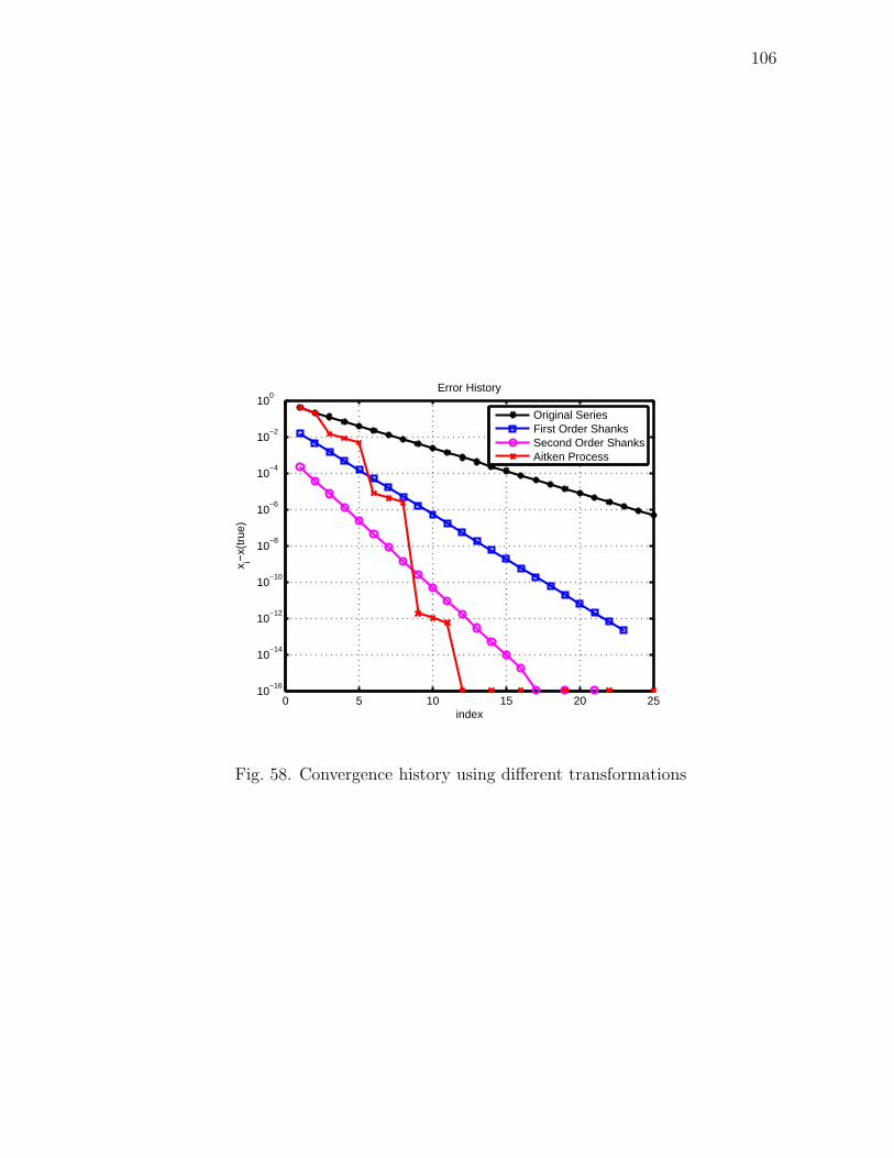
106

0 5 10 15 20 2510

−16

10−14

10−12

10−10

10−8

10−6

10−4

10−2

100

index

x i−x(

true

)

Error History

Original SeriesFirst Order ShanksSecond Order ShanksAitken Process

Fig. 58. Convergence history using different transformations

107

C. The Linearization Approach

For a first order differential equation

dx

dτ= f (τ,x),−1 ≤ τ ≤ 1 (5.10)

the linearization approach generates a sequence of solutions by using the first-order

Taylor expansion of function f . The solution at the ith iteration xi(τ) is related to

the solution at the (i− 1)th iteration xi−1(τ) through the formula

xi(τ) = x(−1) +

∫ τ

−1

(

f (xi−1, s) +∂f

∂x|xi−1(s)(x

i(s)− xi−1(s))

)

ds (5.11)

Note that Eq. 5.11 is different from the original MCPI method in that the solution

xi(τ) appears on both sides of the equation.

Assume that the nth order Chebyshev expansions for the current iteration so-

lution xi(τ), the previous iteration solution xi−1(τ), function f , and the Jacobian

matrix of f , have the following forms

xi(τ) = Σnk=0

′αkTk(τ) (5.12)

xi−1(τ) = Σnk=0

′βkTk(τ) (5.13)

f (xi−1, τ) = Σnk=0

′FkTk(τ) (5.14)

∂f

∂x|xi−1 = Σn

k=0′DkTk(τ) (5.15)

Utilizing the multiplication property of the Chebyshev polynomials

Tm(τ)Tn(τ) =1

2

(

Tm+n(τ) + T|m−n|(τ))

(5.16)

for the second part of the integrand in Eq. 5.11, we may expect that a similar form

of equations for solving for the Chebyshev coefficients can be obtained by using the

same approach through which the original MCPI method is derived. However, com-

108

puting the Jacobian matrix and its Chebyshev approximations can be challenging.

Furthermore, the linearization method couples the coefficient equations for different

states, which can complicate the equations to solve for the coefficients tremendously,

especially for high dimensional problems. We believe a general formula for solving

for the coefficients is difficult to obtain if not impossible. More importantly, solving

the resulting high dimensional equations will be very time-consuming.

We consider a special case which leads to a compact analytical equation for

solving for the Chebyshev coefficients. The ordinary differential equation is a scalar

case problem and all the Chebyshev coefficients Dk in Eq. 5.15 are treated as zero

except the zero order term. Under these assuMCPIions, Eq. 5.11 leads to

1

2α0T0(τ) + α1T1(τ) + α2T2(τ) + · · ·αNTN(τ) =

x(−1) +

∫ τ

−1

(

1

2(F0 +

1

2D0(α0 − β0))T0(s) + ·+ (FN +

1

2D0(αN − βN))TN(s)

)

ds

= x(−1) +1

2(F0 +

1

2D0(α0 − β0))T1(τ) +

1

4(F1 +

1

2D0(α1 − β1))T2(τ) + · · ·

+1

4(FN +

1

2D0(αN − βN ))(

1

N + 1TN+1(τ)−

1

N − 1TN−1(τ)) (5.17)

Including the initial condition x(−1) = x0 and equating the coefficients of the

same order for both sides lead to the following linear equation for solving for the

(N + 1) Chebyshev coefficients

12

−1 1 · · · (−1)N

D0 −4 −D0 0 0

0 D0 −8 −D0 0

......

......

...

0 0 0 D0 −4N

α0

α1

α2

...

αN

=

x0

2(F2 − F0) +D0(β0 − β2)

2(F3 − F1) +D0(β1 − β3)

...

−FN−1 +D0βN−1

(5.18)

In Eq. 5.18, 0 represents a zero vector with the appropriate dimension. Except for the

109

first row and the last row, the subset of the coefficient matrix has a special structure:

the diagonal term of the ith row is −4(i − 1), the entry before the diagonal term is

D0, and the entry after the diagonal term is −D0.

It is interesting to note that Eq. 5.18 is consistent with the equation derived by

Norton [22]. Norton starts the derivation by using the following iteration form

dxi

dτ= f(xi, τ) + (xi − xi−1)

∂f

∂x|xi−1 (5.19)

Equation 5.18 can be generalized to solve BVP using the same assuMCPIions for

Dk. Both the zero and first order coefficients should be constrained by the boundary

conditions.

D. Correction Control MCPI Methods

As shown in Chapter III, MCPI methods are essentially not stable when the domain

of the independent variable is large. However, if we treat the sequence of the solutions

generated from MCPI methods as a dynamic system response, it is possible that there

exist some control algorithms that can manipulate the system behavior such that the

new sequence of the solutions converges to the right solution even though the original

sequence diverges.

Inspired by the proportional control, which is one of the most simple means of

control, a proportional correction control MCPI method is designed as follows. As-

sume the original MCPI method generates a solution x− at the ith step and generates

a new solution x at the (i+ 1)th step, and then the correction control MCPI method

updates the solution at the (i+ 1)th step through

x+ = x− + C(x− x−) (5.20)

110

where C is a matrix that acts like the proportional gain. The matrix C can be

constant or time varying, and can even be adaptively adjusted. Notice that when

C becomes an identity matrix, Eq. 5.20 has the same form as the original MCPI

method.

E. Numerical Examples

1. Characteristics of Convergence of MCPI Methods for Solving IVPs and BVPs

In Chapter III and Chapter IV, we focus on comparing the time efficiency and the

accuracy of MCPI methods with other traditional methods. To illustrate the benefit

of using the three techniques introduced in this chapter for improving the original

MCPI methods, we first look at some convergent characteristics of MCPI methods

when solving IVPs and BVPs.

The two-body problem discussed in Chapter III and the classical Lambert’s prob-

lem presented in Chapter IV are the study cases. Again, the F and G solution provides

a baseline for verifying the obtained results using MCPI methods. For the Lambert’s

problem case, we start by integrating the orbit for some time using some known initial

position r(t0) and velocity v(t0) to obtain a position at the final time as r(tf). Next

we input the positions at the initial time and at the final time r(tf ) as the two-point

boundary conditions, and utilize the MCPI method to solve for the required velocity

at the initial time v(t0). The error of the MCPI method in this case is defined as

|e| = |v(t0) − v(t0)|. For the case that the time of flight is 1/7 of the orbit, the

MCPI method converges in 32 steps and the norm of the initial velocity error is

1.555× 10−13km/s.

Figures 59 and 63 show the relative errors at each iteration for the initial value

problem and the two-point boundary value problem. With a zigzag fashion, the errors

111

are decreasing in a nearly exponential form for both cases. Figures 60 and 64 show the

convergence rate of the errors with respect to the number of the iterations, where the

convergence rate is defined as the ratio of the solution errors between two immediate

iterations. Instead of having a linear form, which is the assuMCPIion for the Aitken

process, the convergence rates are oscillating. Because the stopping criterion chosen

for MCPI methods is based on the corrections between three immediate iterations,

the correction histories and correction rates are also shown in Figs. 61, 62, 65, and 66.

Similar to the error histories, the corrections between each iteration are decreasing

almost exponentially, but the rates of the corrections have oscillating forms.

0 10 20 30 40 5010

−14

10−12

10−10

10−8

10−6

10−4

10−2

100

102

iteration number

|R(M

PC

)−R

(FG

)|m

ax/R

(FG

)

Convergence History: Max Distance Error

Fig. 59. Max relative distance error (IVP)

112

0 10 20 30 40 500

0.5

1

1.5

2

2.5

3

3.5

iteration number

|R(M

PC

)−R

(FG

)|n/|R

(MP

C)−

R(t

rue)

| n−1

Convergence Rate of the Max Distance Error

Fig. 60. Convergence rate of the max distance error (IVP)

0 10 20 30 40 5010

−10

10−8

10−6

10−4

10−2

100

102

104

106

iteration number

corr

ectio

ns

Correction History: Rnew

−Rold

Fig. 61. Norm of the corrections (IVP)

113

0 10 20 30 40 50−10

−8

−6

−4

−2

0

2

4

iteration number

|∆ R

new

−∆

Rol

d|

Correction Convergent Rate

Fig. 62. Correction rate (IVP)

0 5 10 15 20 25 30 3510

−14

10−12

10−10

10−8

10−6

10−4

10−2

100

iteration number

|V0(M

PC

)−V

0(tru

e)|/V

0(tru

e)

Convergence History: Relative Initial Velocity Error

Fig. 63. Relative initial velocity error (BVP)

114

0 5 10 15 20 25 30 350

0.5

1

1.5

2

2.5

iteration number

|Vn(M

PC

)−V

0(tru

e)|/|

Vn−

1(MP

C)−

V0(t

rue)

|

Convergence Rate of the Relative Initial Velocity Error

Fig. 64. Convergence rate of the initial velocity error (BVP)

0 5 10 15 20 25 30 3510

−5

10−4

10−3

10−2

10−1

100

101

102

103

iteration number

|Xne

w−

Xol

d|

Correction History

Fig. 65. Norm of the corrections (BVP)

115

0 5 10 15 20 25 30 350

0.5

1

1.5

2

2.5

iteration number

|∆ X

new

−∆

Xol

d|

Correction Convergent Rate

Fig. 66. Correction rate (BVP)

116

2. Using the Aitken MCPI Methods to Solve Lambert’s Problem

Because Aitken’s process is based on the assuMCPIion that the series converge in a

geometric fashion, we should not expect that utilizing the Aitken’s process for MCPI

methods will always help to achieve significantly better performance. Although the

Picard iteration itself has a geometric convergent behavior [31, 64], the proposed

MCPI method has a much faster convergence rate than the linear form because

Chebyshev polynomials are utilized. A rigorous and general transformation tech-

nique that is well-suited with MCPI methods, which have a hybrid nature of both the

Picard iteration and Chebyshev polynomials, currently does not exist. But Aitken’s

process does appear to improve the convergence performance of MCPI methods.

We compare the performance of the original MCPI method and the Aitken MCPI

method for Lambert’s problem. The interval lengths are chosen from

0.1, 0.2. 0.3, 0.34, 0.35, 0.36, 0.37Tp where Tp is the orbital period. The required

iteration numbers are shown in Fig. 67 and the CPU times are shown in Fig. 68.

These plots show that, as the interval length increases, the benefit of using Aitken’s

process becomes more significant because it reduces both the number of iterations

and CPU time. For the case where the interval length is 0.37Tp, the CPU time of the

MCPI method is two times the CPU time of the Aitken MCPI method and requires

about three times of iterations. Additionally, when the time interval increases to

0.38Tp and 0.39Tp, the original MCPI method diverges but the Aitken MCPI method

converges after 282 and 432 iterations respectively.

117

0.1 0.15 0.2 0.25 0.3 0.35 0.4 0.450

100

200

300

400

500

600

700

Interval length(t/Tp)

Itera

tion

num

bers

Iteration numbersMCPIAitken MCPI

Fig. 67. Iteration number comparison (BVP)

0.1 0.15 0.2 0.25 0.3 0.35 0.4 0.450

0.02

0.04

0.06

0.08

0.1

0.12

0.14

Interval length(t/Tp)

CP

U(s

ec)

CPU TimeMCPIAitken MCPI

Fig. 68. CPU time comparison (BVP)

118

3. Using the Linearization MCPI Methods to Solve a Linear Problem

To satisfy the assuMCPIions in Eq. 5.18, we consider an initial value problem

dx

dt= −λx, t ∈ [0, Tf ] (5.21)

with an initial condition x(0) = 1. The analytical solution is x(t) = e−λt.

For the case when Tf = 5 seconds and λ = 5, the errors of the solutions using

the MCPI method and the linearization MCPI method are shown in Figs. 69 and 70.

The original MCPI method takes 333 iterations to find the solution in 0.02 seconds,

whereas the linearization MCPI method takes 37 iterations to find the solution in

0.1 seconds. The order of the Chebyshev polynomial is chosen as 100 and the direct

inversion approach is used to solve for the coefficients with Eq. 5.18. Although fewer

iterations are required for the linearization MCPI method, solving the linear equations

takes additional time, which causes the CPU time for the linearization MCPI method

to be larger than the CPU time for the original MCPI method. However, increasing

the final time Tf to ten seconds causes the original MCPI method to diverge, whereas

the linearization MCPI method finds the solution using 58 iterations in 0.14 seconds.

The solution errors are shown in Fig. 71.

119

0 1 2 3 4 5−4

−2

0

2

4

6

8

10

12

14x 10

−9 ∆ x

time(sec)

x(M

PC

)−x(

true

)

Fig. 69. Error history of the MCPI method (Tf = 5s)

0 1 2 3 4 5−8

−7

−6

−5

−4

−3

−2

−1

0

1x 10

−9 ∆ x

time(sec)

x(lin

eariz

atio

n M

PC

)−x(

true

)

Fig. 70. Error history of the linearization MCPI method (Tf = 5s)

120

0 2 4 6 8 10−1

0

1

2

3

4

5

6

7

8x 10

−9 ∆ x

time(sec)

x(lin

eariz

atio

n M

PC

)−x(

true

)

Fig. 71. Error history of the linearization MCPI method (Tf = 10s)

121

4. Using Correction Control MCPI Methods to Solve IVPs and BVPs

For the two-body problem discussed in Chapter III, the original MCPI method failed

to converge after 1000 iterations using polynomials of order 400 and the stopping

criterion of 10−6,. Figure 72 shows that the corrections of the sequence generated

from the MCPI method are oscillating after about 200 iterations and the accuracy

no longer improves. The relative position errors after the 1000 iterations are shown

in Fig. 73. Choosing all the diagonal terms of the C matrix in Eq. 5.20 as 0.7,

the correction control MCPI method converges after 240 iterations. This correction

history is shown in Fig. 74, and the final relative position errors are shown in Fig. 75.

0 200 400 600 800 100010

−2

100

102

104

106

108

Iterations

|Xi−

Xi−

1|

Correction History

Fig. 72. Correction history using MCPI

122

0 0.5 1 1.5 2 2.5 3 3.5 4−0.02

0

0.02

time (t/Tp)

∆ x

Relative position errors from MPC (based on FG soln)

0 0.5 1 1.5 2 2.5 3 3.5 4−2

0

2x 10

−4

time (t/Tp)

∆ y

0 0.5 1 1.5 2 2.5 3 3.5 4−5

0

5x 10

−3

time (t/Tp)

∆ z

Fig. 73. Relative position errors using MCPI

0 50 100 150 200 25010

−4

10−2

100

102

104

106

108

Iterations

|Xi−

Xi−

1|

Correction History

Fig. 74. Correction history using correction control MCPI

123

0 0.5 1 1.5 2 2.5 3 3.5 4−5

0

5x 10

−6

time (t/Tp)

∆ x

Relative position errors from MPC (based on FG soln)

0 0.5 1 1.5 2 2.5 3 3.5 4−2

0

2x 10

−6

time (t/Tp)

∆ y

0 0.5 1 1.5 2 2.5 3 3.5 4−1

0

1x 10

−5

time (t/Tp)

∆ z

Fig. 75. Relative position errors using correction control MCPI

124

The Earth to Apophis optimal trajectory design problem is used here again to

illustrate the benefit of using the correction control MCPI method to solve BVP.

The original MCPI method only converges when the time of flight is no longer than

110 days. The correction control MCPI method expands this convergence domain

significantly. Here the solution can be found for a time of flight of 150 days when the

feedback gain C is chosen as a constant diagonal matrix with all the diagonal terms

set to be 0.7. For this case, SNOPT converges in approximately five seconds with

the boundary condition errors of magnitude 10−8. The homotopy method finds the

solution in seven and half seconds with the boundary condition errors of magnitude

10−13. The MCPI method takes significantly less time to converge: 0.3 seconds in 226

iterations. Figures 76 to 81 show that the errors of the solutions for both the states

and co-states are within the boundary of 10−9.

0.5

1

1.5

30

210

60

240

90

270

120

300

150

330

180 0

α=0.007487

Earth orbitApophis OrbitTransfer OrbitThrust directionEarth InitialEarth FinalApophis InitialApophis Final

Fig. 76. Transfer orbit with time of flight 150 days

125

0 0.5 1 1.5 2 2.5 3−0.5

0

0.5

1

1.5

2

2.5

3

3.5

4x 10

−9

time(TU)

r(M

PC

)−r(

true

)

Error of the Radius(AU)

Fig. 77. Error of the radius (150 days)

0 0.5 1 1.5 2 2.5 3−4.5

−4

−3.5

−3

−2.5

−2

−1.5

−1

−0.5

0

0.5x 10

−9

time(TU)

θ(M

PC

)−θ(

true

)

Error of the Phase Angle(rad)

Fig. 78. Relative error of the phase angle (150 days)

126

0 0.5 1 1.5 2 2.5 3−12

−10

−8

−6

−4

−2

0

2

4x 10

−9

time(TU)

u(M

PC

)−u(

true

)

Error of u(AU/TU)

Fig. 79. Error of the radial velocity (150 days)

0 0.5 1 1.5 2 2.5 3−12

−10

−8

−6

−4

−2

0

2

4

6x 10

−9

time(TU)

v(M

PC

)−v(

true

)

Error of v(AU/TU)

Fig. 80. Error of the tangential velocity (T150 days)

127

0 0.5 1 1.5 2 2.5 3−0.5

0

0.5

1

1.5

2

2.5x 10

−7

time(TU)

(β(M

PC

)−β(

true

)

Error of the Thrust Angle(rad)

Fig. 81. Error of the thrust angle (150 days)

0 0.5 1 1.5 2 2.5 3−6

−4

−2

0

2

4

6

8x 10

−9

time(TU)

\lam

da_r

(MP

C)−

\lam

bda_

r(tr

ue)

Error of the Costates of Radius

Fig. 82. Error of the costate about radius (150 days)

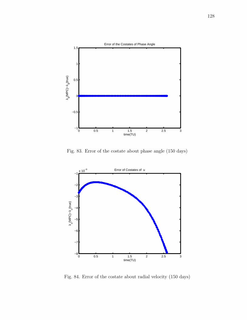
128

0 0.5 1 1.5 2 2.5 3−1

−0.5

0

0.5

1

1.5

time(TU)

λ θ(MP

C)−

λ θ(tru

e)

Error of the Costates of Phase Angle

Fig. 83. Error of the costate about phase angle (150 days)

0 0.5 1 1.5 2 2.5 3−8

−7

−6

−5

−4

−3

−2

−1x 10

−9

time(TU)

λ u(MP

C)−

λ u(tru

e)

Error of Costates of u

Fig. 84. Error of the costate about radial velocity (150 days)

129

0 0.5 1 1.5 2 2.5 31

2

3

4

5

6

7

8

9

10

11x 10

−9

time(TU)

λ v(MP

C)−

λ v(tru

e

Error of Costates of v

Fig. 85. Error of the costate about tangential velocity (150 days)

130

Similar to the importance of proportional gain in control of dynamic system

behaviors, the gain matrix C is a key factor affecting the convergence behavior of

the correction control MCPI method. Figure 86 shows the required iterations for

different diagonal gain values, and Fig. 87 shows the CPU time for different chosen

gains. These plots show that increasing the gain reduces both the number of iterations

and the CPU time. However, too large of a gain will cause the methods to diverge

again.

0.1 0.2 0.3 0.4 0.5 0.6 0.7 0.8100

150

200

250

300

350

400

450

500

550

600

C: Control Gain

Itera

tions

Iterations Numbers

Fig. 86. Iteration number comparison (150 days)

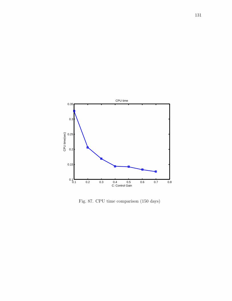
131

0.1 0.2 0.3 0.4 0.5 0.6 0.7 0.80.1

0.15

0.2

0.25

0.3

0.35

C: Control Gain

CP

U ti

me(

sec)

CPU time

Fig. 87. CPU time comparison (150 days)

132

F. Summary

Although Aitken’s process is designed for linearly convergent sequences, it is capa-

ble of improving MCPI methods, which do not converge in a geometrical fashion.

The linearization approach can extend the convergence domain for the original MCPI

methods, but it is difficult to apply to high-dimension nonlinear problems. The pro-

portional correction control method is a very simple technique that can enlarge the

convergence domain significantly. We suspect that more advanced control methodol-

ogy can further enlarge the convergence domain. Such schemes may include choosing

an optimal gain matrix that can vary during the iteration process as well as design-

ing some more advanced control methods. Up through this chapter, all the numerical

results have been obtained using the serial computation in MATLAB. The next chap-

ter will discuss implementing MCPI methods on a graphics card, which provides a

parallel computation environment for testing the proposed MCPI methods.

133

CHAPTER VI

IMPLEMENTATION OF MCPI METHODS USING GRAPHICS PROCESSING

UNITS

A. Introduction

In Chapter III and Chapter IV, MCPI methods were shown to achieve both improved

accuracy and significant speedup when solving IVPs and BVPs in a serial computa-

tion environment. Due to the parallel structure of the methods, additional speedup

is expected when the serial implementations are extended to a parallel computation

environment. However, to achieve the most potential from using the parallel pro-

cessors, the structure of the algorithm must be complementary to the architecture

of the hardware. As warned by Thurber and Wald, any atteMCPI to use a parallel

computer with the wrong type of problems or methods is an exercise in futility [65].

Possible computer architectures can be classified into the following four categories

according to the taxonomy introduced by Flynn [66].

• Single Instruction, Single Data stream (SISD): the computer architecture in

which a single instruction is operated on a single stream of data. This type is

basically the sequential computer where no parallelism is used.

• Single Instruction, Multiple Data streams (SIMD): the computer architecture

in which a single instruction is operated on multiple streams of data simultane-

ously. One example of this type is the Graphics Processing Unit (GPU).

• Multiple Instruction, Single Data stream (MISD): the computer architecture in

which multiple instructions are operated on single stream of data. This type of

computer is mostly used for fault tolerance.

134

• Multiple Instruction, Multiple Data streams (MIMD): the computer architec-

ture in which multiple instructions are operated on multiple streams of data

simultaneously. One example of this type is the distributed system.

The proposed MCPI methods are well suited for large-scale data parallelism. Dis-

tributing the computation of both the force function evaluation at different time

nodes and the coefficients of the Chebyshev polynomials for different orders to mul-

tiple processors is straightforward. Speedup is achieved when MCPI methods are

implemented on SIMD type of parallel computers. For problems such as maintaining

satellite catalog (see Chapter I) in which the force functions are highly computation-

ally expensive and the dynamic systems require high order Chebyshev polynomials

to approximate, significant speedups can be obtained.

Because of its rapid development and inexpensive price, the NVIDIA graphics

card, one type of SIMD hardware, is chosen as the hardware for implementing MCPI

methods in a parallel environment. This chapter first introduces GPU technology and

discusses existing methods that use NVIDIA GPUs to solve IVPs. Next, the Compute

Unified Device Architecture (CUDA) environment and CUBLAS (an implementation

of the Basic Linear Algebra Subprograms (BLAS) on top of the NVIDIA CUDA)1 are

presented. The approach using CUDA and CUBLAS to implement MCPI methods is

then presented. The performance of the graphic card first is tested with a matrix mul-

tiplication problem. We then present the results obtained using the GPU-accelerated

MCPI methods to solve the small perturbation from the sinusoid motion problem and

the zonal harmonic perturbation involved satellite motion propagation problem.

1http://developer.nvidia.com/object/gpucomputing.html [retrieved May 7, 2010]

135

B. NVIDIA Graphics Processing Units

GPUs are traditionally specialized for three-dimensional graphics real-time rendering.

Their highly parallel structure makes them more effective than the general-purpose

CPU for parallel computation. With the recent programmability enhancements as-

sociated with some development environment such as NVIDIA CUDA, GPUs have

helped to solve complicated scientific computation problems in various fields such as

molecular modeling, magnetic resonance imaging, N-body simulations, and evolution-

ary algorithms [67, 68, 69, 70]. NVIDIA GPUs represent the state of the art of General

Purpose GPUs (GPGPU). The NVIDIA GPU consists of a set of multiprocessors that

can be used by the graphic cards to solve many complicated computational problems

in addition to the traditional 3D graphics functions.

One important reason for the successful application of GPUs to these problems is

the amazing rate at which the GPU technology is developing, dwarfing even Moore’s

law that applies broadly to advances in computer hardware and computing speed.

GPU-accelerated computational power nearly doubles every six months while CPU

computational power doubles about every 18 months [71]. GPUs are relatively inex-

pensive; their competitive price is mainly due to mass production related to the high

demand of the commercial gaming industry. As a consequence, we have entered the

age of personal supercomputing, and it is possible to run large complicated problems

on a personal computer. Previously this was impractical due to the lengthy processing

time required. For example, the current GeForce GTX 280 GPU achieves 141.7GB/s

memory bandwidth and 933 Giga Floating point Operations Per Second (GFLOPS)

for single-precision computation. Thus, a 0.93 Terraflop personal computer is now

available through the addition of a graphics card costing only a few hundred dollars.

Most current GPU-based applications for solving IVPs use simple forward in-

136

tegration algorithms for dynamic system simulations such as the first-order Euler

integration method or the second-order leapfrog-Verlet integrator [72]. However, the

accuracy of these low-order integration methods is often low. Therefore we must

extend beyond these elementary applications and consider more powerful differential

equation solvers. Additionally, both Euler and leapfrog-Verlet methods are essen-

tially sequential, not parallel algorithms. Although when solving an all-pairs N-body

problem by using the GPU techniques [72], Nyland et al. have achieved 50 times as

fast as a highly tuned serial implementation or 250 times faster than a portable C im-

plementation, it is safe to predict that an efficient parallelized integration algorithm

such as the proposed MCPI methods can further improve the overall performance.

C. CUDA Environment and CUBLAS Toolbox

CUDA is a general purpose parallel computing architecture developed by NVIDIA2.

It is the computing engine that allows developers to use NVIDIA GPUs to conduct

high performance computations. The programming mode of CUDA includes kernels,

blocks, and threads. A kernel is executed as a grid of blocks, and a block is a

batch of threads that can cooperate with each other by sharing data through shared

memory. Threads belonging to one block can execute synchronically while threads

belonging to different blocks can not cooperate. Since NVIDIA GPUs are based on

SIMD architecture, CUDA achieves its best performance when a single operation is

running simultaneously on many threads, which is well-suited for MCPI methods.

Compared with CPU threads, CUDA threads are extremely lightweight with little

creation overhead and can be switched instantly. Furthermore, while multi-core CPUs

usually can have only a few threads, the current maximum number of threads for one

2http://developer.nvidia.com/object/gpucomputing.html [retrieved May 7, 2010]

137

grid on a graphics card is tens of thousands.

The CUDA environment provides two levels of application programming interface

(API) functions: a low-level CUDA driver API and a high-level CUDA runtime API.

These APIs provide five categories of functions for users to use: general functions

such as the clock function and the standard math functions, device functions, memory

management functions, flow control functions, and interface functions with OpenGL

and Direct3D.

CUDA code is compiled by the NVIDIA C Compiler (NVCC). The code that

runs on the CPU is called the host code and the code that runs on the GPU is called

the device code. The NVCC separates the host code to its own compiler and links

it with the compiled device code during the run time. To achieve the most potential

using CUDA, in addition to a good knowledge of the general parallel computation

theory, the developers need to understand some specific characteristics of the CUDA

performance. For examples, the developers should take advantage of the much faster

shared memory rather than the global memory, use memory coalescing to reduce

latency, and optimize the program to avoid memory bank conflicts and divergent

branching issues.

Three levels of BLAS functions are included in CUBLAS. Level one is for scalar,

vector, and vector-vector operations; level two is for vector-matrix operations; and

level three is for matrix-matrix operations. The CUBLAS toolbox includes both single

precision functions and double precision functions. Users should make sure that the

computing capability of their graphic cards is at least 1.3 in order to use the double

precision functions correctly. Notice that the functions in CUBLAS are not always the

fastest realization of the algorithms because they are written for many possible cases.

For example, the matrix multiplication function cublasSgemm considers additional

cases where one or two of the input matrices are transposed, the multiplication result

138

is multiplied by a scalar, and another summation is involved. Still we choose to use

CUBLAS because the implemented functions have been tested on different graphic

cards and are robust to various programming errors.

The way we implement MCPI method is shown in Fig. 88, where GPU denotes

the code is running on the device (graphics card), CPU denotes the code is running

on the host, and CUBLAS denotes the CUBLAS toolbox is used to do the compu-

tation. Notice that the coefficient matrices Cx and Cα are constant once the order of

polynomials is defined. They are calculated before the iteration starts.

Starting Guess

Coefficient Update

Constant Matrix Initialization

Force Evaluation

xCC

oldx

xnewCx

oldnewnewxxe

?new

e

?old

eand existExit

newoldxx

newoldee

Iterate

YESNO

(CUBLAS)

(GPU)

(CUBLAS)

(CUBLAS)

(CUBLAS)

(GPU) (CPU)

Fig. 88. Implementation of MCPI methods using CUDA and CUBLAS

D. Graphic Card Testing

The settings of the computer and the development environment used are the following

139

• Intel(R) Pentium(R) D CPU 3.4GHz, 3.4GHz, 2.0GB of RAM

• Windows XP Operating System

• NVIDIA GeForce 9400GT Graphics Card

• MATLAB R2009b

• Microsoft Visual Studio 2005

The theoretical memory bandwidth for GeForce 9400GT is 12.8 GB/s and the peak

GFLOPS is 67.2 for single precision computation. The runtime example of a single

precision matrix multiplication indicates that the bandwidth is 7.9419GB/s, and the

maximum GFLOPS is 25.

Due to the vector-matrix characteristic form of MCPI methods, we compare the

performance of three different computation environments for matrix multiplication

first. The results are shown in Table I, where

• N: dimension of the square matrices

• MB(A+B+C): size of A+B+C in Megabytes

• MT: MATLAB computation time

• h2d: data transfer time from the host to the device

• kernel: computation time using cublasSgemm function

• d2h: data transfer time from the device to the host

• serial−CGPU

: ratio of the computation time between that of the serial C code and

cublasSgemm

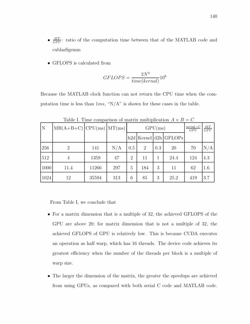
140

• MTGPU

: ratio of the computation time between that of the MATLAB code and

cublasSgemm

• GFLOPS is calculated from

GFLOPS =2N3

time(kernal)106

Because the MATLAB clock function can not return the CPU time when the com-

putation time is less than 1ms, “N/A” is shown for these cases in the table.

Table I. Time comparison of matrix multiplication A×B = C

N MB(A+B+C) CPU(ms) MT(ms) GPU(ms) serial−CGPU

MTGPU

h2d Kernel d2h GFLOPs

256 2 141 N/A 0.5 2 0.3 20 70 N/A

512 4 1359 47 2 11 1 24.4 124 4.3

1000 11.4 11266 297 5 184 3 11 62 1.6

1024 12 35594 313 6 85 3 25.2 419 3.7

From Table I, we conclude that

• For a matrix dimension that is a multiple of 32, the achieved GFLOPS of the

GPU are above 20; for matrix dimension that is not a multiple of 32, the

achieved GFLOPS of GPU is relatively low. This is because CUDA executes

an operation as half warp, which has 16 threads. The device code achieves its

greatest efficiency when the number of the threads per block is a multiple of

warp size.

• The larger the dimension of the matrix, the greater the speedups are achieved

from using GPUs, as compared with both serial C code and MATLAB code.

141

The speedups of using GPU over MATLAB are three to four for the matrix

dimension that is a multiple of 32; the speedups of using GPU over serial C

code are in the range of 60 to 400.

E. GPU-Accelerated MCPI Methods for Solving the Small Perturbation from the

Sinusoid Motion Problem

1. Sequential MCPI and GPU-accelerated MCPI in C

Here we choose the small perturbation from the sinusoid motion discussed in Chap-

ter III as a case study. The results are shown in Table II, where

• N: order of the polynomials

• Cx, Cα: computation time for the two constant matrices

• Iteration: computation time during the iterations

• h2d: matrix transferring time from the host to the device

• d2h: matrix transferring time from the device to the host

• Overall: total computation time: h2d+(Cx, Cα)+ iteration+d2h

Table II. Time comparison of sequential MCPI and GPU-accelerated MCPI in C

N CPU time(ms) GPU time(ms) CPUGPU

Cx, Cα Iteration Overall h2d Cx, Cα Iteration d2h Overall

511 5391 16 5407 4 43 4 0.3 51 106

1000 57766 125 57891 11 747 29 0.3 787.3 73.5

1023 163797 156 163953 12 340 8 0.3 360.3 455

142

Table II shows that

• For the largest polynomials of order 1023, which are beneficial to CUDA com-

putation, the speedups achieved by using the GPU are more than four hundred.

• The matrix multiplication operation is the dominate cause for these speedups.

• The speedup from the iteration part is about four for N = 511 and N = 1000;

for N = 1023 the gain is about twenty.

2. GPU-Accelerated MCPI in C and Sequential MCPI in MATLAB

Because the vector and matrix operations using the CPU are developed “in-house”,

they may be significantly less efficient than the BLAS functions. Thus, the previous

comparison is biased to the GPU implementation. Because the vector and matrix op-

erations in MATLAB are highly efficient, we choose to compare the implementation

of MCPI methods between using GPU in C environment and using sequential MAT-

LAB with single precision calculation. Table III shows that the speedups achieved

by using the GPU card over the MATLAB implementation are in the range of 2 to

4.5. From Table III, some important conclusions can be drawn, such as

Table III. Time comparison of sequential MCPI in MATLAB and GPU-accelerated

MCPI in C

N MATLAB time(ms) GPU time(ms) MTGPU

Cx, Cα Iteration Overall h2d Cx, Cα Iteration d2h Overall

511 219 N/A 219 4 43 4 0.3 51 2

1000 1531 51 1582 11 747 29 0.3 787.3 2.0

1023 1578 31 1609 12 340 8 0.3 360.3 4.5

143

• The higher the order of polynomials, the greater the gain can be obtained from

using the GPU implementation.

• For the matrix size which lends itself to GPU computation, the speedup ac-

complished by using GPU is even higher. When the order of the polynomial is

chosen to be 1023, which leads to the matrix size of 1024, the greatest speedup

results.

F. GPU-accelerated MCPI Methods for Zonal Harmonic Perturbation Involved Satel-

lite Motion Propagation Problems

The zonal harmonic perturbation satellite motion propagation problem discussed in

Chapter III is chosen as another study case. The simulation results are shown in

Figs. 89 to 93. Several important observations are

• As can be seen from Figs. 89 and 90, compared with the sequential code in

MATLAB, the computation time required by the GPU-accelerated MCPI code

in C does not change significantly when higher order zonal harmonic perturba-

tions are included.

• Figures 91 and 92 show that the speedups obtained from the GPU-accelerated

MCPI code increase as either the perturbation forces become more complicated

or higher order polynomials are used.

• Figure 93 shows the relative differences of the solutions between these two im-

plementations are below 10−6. Considering the graphic card we use is only

capable of single precision computation, we expect the two obtained solutions

will match better once we implement the GPU-accelerated MCPI code using an

advanced card that can conduct double precision computation.

144

1 1.5 2 2.5 3 3.5 4 4.5 50

10

20

30

40

50

60

70

80

90


CP

U(m

s)

CPU time comparision (N=127)

MatlabGPU accerated C

Fig. 89. Computation time of GPU-accelerated MCPI and MATLAB MCPI (N=127)

1 1.5 2 2.5 3 3.5 4 4.5 50

100

200

300

400

500

600


CP

U(m

s)

CPU time comparision (N=511)

MatlabGPU accerated C

Fig. 90. Computation time of GPU-accelerated MCPI and MATLAB MCPI (N=511)

145

1 1.5 2 2.5 3 3.5 4 4.5 56

7

8

9

10

11

12

13

14

15

16


CP

U(M

AT

LAB

)/C

PU

(GP

U)

Speedups from GPU (N=127)

Fig. 91. Speedup of GPU-accelerated MCPI over MATLAB MCPI (N=127)

1 1.5 2 2.5 3 3.5 4 4.5 522

24

26

28

30

32

34

36


CP

U(M

AT

LAB

)/C

PU

(GP

U)

Speedups from GPU (N=511)

Fig. 92. Speedup of GPU-accelerated MCPI over MATLAB MCPI (N=511)

146

0 100 200 300 400 500 60010

−10

10−8

10−6

time (sec)

∆ x

Relative difference of x

0 100 200 300 400 500 60010

−10

10−8

10−6

time (sec)

∆ y

Relative difference of y

0 100 200 300 400 500 60010

−10

10−8

10−6

time (sec)

∆ z

Relative difference of z

Fig. 93. Relative position difference between GPU-accelerated MCPI and MATLAB

MCPI (N=511)

147

G. Summary

The recently developed GPU technology provides a SIMD parallel architecture for

implementing MCPI methods. Although how much speedup can be achieved from

the parallel implementation will depend on the problems themselves, this chapter has

showed the power of parallel implementation of serial MCPI methods. For the small

perturbation from the sinusoid motion problem where the force function is relatively

simple, the speedups gained by using GPUs over the reference MATLAB solutions are

in the range of two to five. For the satellite motion propagation problems, the more

complicated the force functions and the higher order polynomials used, the larger the

speedups that are achieved when using GPUs. The largest speedup for this study is

34.6, which is obtained when we use 511th order Chebyshev polynomials and include

up to 5th order zonal harmonic perturbations.

148

CHAPTER VII

CONCLUSIONS

This dissertation has presented a unified framework for applying MCPI methods

to solve IVPs and BVPs. The accuracy, efficiency, and parallel structure of MCPI

methods are illustrated through several important celestial mechanics problems.

For IVPs, MCPI methods solve problems over arbitrary finite time intervals us-

ing a piecewise approach. For the small perturbation from the sinusoid motion and

the satellite motion propagation problems, MCPI methods achieve better accuracy

and speedups when compared with ODE45 in MATLAB, even prior to parallel im-

plementation. Larger speedups are obtained when MCPI methods are implemented

using GPU technology. The following two techniques have been shown to further

speed up MCPI methods:

1. To solve IVPs with systems that are described by higher-order differential equa-

tions, MCPI methods do not require transforming the original equations to their

first-order forms. MCPI methods can solve for the lower-order states directly

without the need to integrate the higher-order information during iterations.

The higher-order information can be obtained conveniently afterwards by using

the properties of Chebyshev polynomials.

2. For IVPs that can be treated as perturbed motion from a reference trajectory,

using MCPI methods to solve for the perturbation motion reduces the compu-

tation time while maintaining the solution accuracy.

For BVPs, MCPI methods find solutions that satisfy both dynamic equation con-

straints and boundary conditions with high accuracy. Compared with several other

BVP solvers, MCPI methods are computationally efficient and not initial guess sen-

149

sitive. Using MCPI methods to solve optimal control problems through Pontryagin’s

principle, optimality and accuracy are guaranteed. For the cases where MCPI meth-

ods diverge, the proposed nonlinear transformations, the linearization approach, and

correction control methods help to enlarge the convergence domain.

As one motivation for this study is the space catalog problem, we summarize the

following results obtained when MCPI methods are used to solve the satellite motion

propagation problems:

1. MCPI methods can integrate the satellite motion for arbitrarily long times.

When compared with ODE45 in MATLAB, the longer the integration time, the

larger the speedups achieved by MCPI methods.

2. To integrate the satellite motion for sixteen revolutions with only the inverse-

square gravity field, using MCPI methods, one achieves up to three orders of

magnitude better accuracy with more than one magnitude of speedups over

ODE45 prior to parallel implementation. MCPI methods that only integrate

position states, obtaining the velocity information afterwards, achieve up to two

orders of magnitude speedups over ODE45.

3. Although the speedup of the sequential realization of MCPI methods drops

when the degree of the included zonal harmonic perturbation forces increase, a

GPU implementation results in significant speedups.

Considering that both sufficient accuracy and significant speedups are accomplished

by the proposed MCPI methods prior to parallel implementation, and that paral-

lel implementation achieves larger speedups when the force functions become more

complicated and higher order polynomials are used to approximate the solutions, we

claim that utilizing MCPI methods results in both accuracy and efficiency for solving

satellite motion propagation problems.

150

With the advantages of MCPI methods in solving IVPs and BVPs, as shown in

the dissertation, the proposed MCPI methods, especially given their inherently paral-

lel structure, will contribute significantly to dynamic system analysis and controlling.

Some suggestions for the future study include the following three fields:

1. Although the current study has shown that a parallel implementation of MCPI

methods brings speedups over forward integration methods, further study could

focus on specific applications and likely achieve even greater speedups than what

we have obtained in this dissertation. For the space catalog mission, integrating

the motion for 150, 000 satellites requires another level of parallelism. Advanced

graphic cards and other more powerful parallel computation environments such

as clusters or distributed computing should be studied. Although this dis-

sertation has provided some insight on how to choose the segment step size,

polynomial order, and stopping criterion, these issues should be further studied

for specific applications to achieve the potential of the MCPI methodology.

2. Through the optimal trajectory design problem, we have shown that once MCPI

methods converge, they solve the problem more than one magnitude faster than

several other popular optimizers prior parallel implementation. Considering the

importance of integrating the dynamic systems when solving optimal control

problems with Pontryagin’s principle and the fact that MCPI methods are very

efficient in solving IVPs, the superior performance of MCPI methods is not

surprising. More efficiency is obtained because MCPI methods do not require

gradient information for solving BVPs. The potential of MCPI methods for

solving optimal control problems with the inherently parallel structure is huge.

In addition to using MCPI methods to solve other types of optimal control

problems, further study could focus on developing more powerful strategies for

151

enlarging the convergence domain.

3. It is through utilizing Chebyshev polynomials that the traditional Picard it-

erations converge fast, compute efficiently, and acquire a parallel structure.

However, these characteristics could also be obtained by using other orthogo-

nal basis functions. Developing a general strategy where Picard iterations are

combined with other basis functions is valuable, as different basis functions

may have different convergence properties. It is possible that for some specific

problems, using one set of basis functions makes the Picard iteration diverge

while using another set of basis functions leads to a converged Picard iteration.

Furthermore, as has been shown, choosing a good reference trajectory and inte-

grating only the perturbation motion will speed up the original MCPI methods.

Similarly, choosing an appropriate basis function for a specific application will

also contribute to greater speedups.

152

REFERENCES

[1] C. W. Gear, “Parallel methods for ordinary differential equations,” Calcolo, vol.

25, no. 1-2, pp. 1–20, Mar. 1988.

[2] M. A. Franklin, “Parallel solution of ordinary differential equations,” IEEE

Transactions on Computers, vol. 27, no. 5, pp. 413–420, May 1978.

[3] W. L. Miranker and W. Liniger, “Parallel methods for the numerical integration

of ordinary differential equations,” Mathematics of Computation, vol. 21, no.

99, pp. 303–320, Jul. 1969.

[4] A. Migdalasa, G. Toraldo, and V. Kumar, “Nonlinear optimization and parallel

computing,” Parallel Computing, vol. 29, no. 4, pp. 375–391, Apr. 2003.

[5] R. Travassos and H. Kaufman, “Parallel algorithms for solving nonlinear two-

point boundary-value problems which arise in optimal control,” Journal of Op-

timization Theory and Applications, vol. 30, no. 1, pp. 53–71, 1980.

[6] J. T. Betts and W. Huffman, “Trajectory optimization on a parallel processor,”

Journal of Guidance, Control, and Dynamics,, vol. 14, no. 2, pp. 431–439, Mar.-

Apr. 1991.

[7] E. Picard, “Sur l’application des mbthodes d’approximations successives b

l’8tude de certaines bquatioiis differentielles or- dinaires,” J. de Math., vol.

9, pp. 217–271, 1893.

[8] E. Picard, Trait d’analyse, vol. 1, chapter 4.7, Paris, France: Gauthier-Villars,

3rd edition, 1922.

153

[9] J. V. Craats, “On the region of convergence of Picard’s iteration,” ZAMM-

Journal of Applied Mathematics and Mechanics, vol. 52, no. 8, pp. 487–491,

Dec. 1971.

[10] F. Lettenmeyer, “Ober die von einem punkt ausgehenden integralkurven einer

differentialgleichung 2. ordnung,” Deutsche Math, vol. 7, pp. 56–74, 1944.

[11] R. P. Agarwal, “Nonlinear two–point boundary value problems,” Indian Journal

of Pure and Applied Mathematics, vol. 4, pp. 757–769, 1973.

[12] W. J. Coles and T. L. Sherman, “Convergence of successive approximations

for nonlinear two-point boundary value problems,” SIAM Journal on Applied

Mathematics, vol. 15, no. 2, pp. 426–433, Mar. 1967.

[13] P. B. Bailey, “On the interval of convergence of Picard’s iteration,” ZAMM

- Journal of Applied Mathematics and Mechanics, vol. 48, no. 2, pp. 127–128,

1968.

[14] P.l Bailey, L. F. Shampine, and P. Waltman, “Existence and uniqueness of

solutions of the second order boundary value problem,” Bulletin of the American

Mathematical Society, vol. 72, no. 1, pp. 96–98, 1966.

[15] M. Urabe, “An existence theorem for multi-point boundary value problems,”

Funkcialaj Ekvacioj, vol. 9, pp. 43–60, 1966.

[16] R. Shridharana and R. P. Agarwal, “General iterative methods for nonlinear

boundary value problems,” The Journal of the Australian Mathematical Society.

Series B. Applied Mathematics, vol. 37, pp. 58–85, 1995.

[17] G. E. Parker and J. S. Sochacki, “Implementing the Picard iteration,” Neural,

Parallel & Scientific Computations, vol. 4, no. 1, pp. 97–112, 1996.

154

[18] L. Fox and I. B. Parker, Chebyshev Polynomials in Numerical Analysis, London,

UK: Oxford University Press, 1972.

[19] C. W. Clenshaw, “The numerical solution of linear differential equations in

Chebyshev series,” Mathematical Proceedings of the Cambridge Philosophical

Society, vol. 53, pp. 134–149, 1957.

[20] R. E. Scraton, “The solution of linear differential equations in Chebyshev series,”

The Computer Journal, vol. 8, no. 1, pp. 57–61, 1965.

[21] K. Wright, “Chebyshev collocation methods for ordinary differential equations,”

The Computer Journal, vol. 6, no. 4, pp. 358–365, 1964.

[22] H. J. Norton, “The iterative solution of non-linear ordinary differential equations

in Chebyshev series,” The Computer Journal, vol. 7, no. 2, pp. 76–85, 1964.

[23] M. Urabe, “Galerkin’s procedure for nonlinear periodic systems,” Archive for

Rational Mechanics and Analysis, vol. 20, no. 2, pp. 120–152, Jan. 1965.

[24] M. Urabe and A. Reiter, “Numerical computation of nonlinear forced oscillations

by Galerkin’s procedure,” Journal of Mathematical Analysis and Application,

vol. 14, no. 1, pp. 107–140, 1966.

[25] B. Chen, R. Garca-Bolsb, L. Jdarb, and M.D. Rosellb, “Chebyshev polyno-

mial approximations for nonlinear differential initial value problems,” Nonlinear

Analysis, vol. 63, no. 5-7, pp. 629–637, 2005.

[26] M. Urabe, “Numerical solution of multi-point boundary value problems in

Chebyshev series theory of the method,” Numerische Mathematik, vol. 9, pp.

341–366, 1967.

155

[27] J. Vlassenbroeck and R. V. Dooren, “A Chebyshev technique for solving non-

linear optimal controlproblems,” IEEE Tansactions on Automatic Control, vol.

33, no. 4, pp. 333–340, Apr. 1988.

[28] M. El-Kady and E. M. E. Elbarbary, “A Chebyshev expansion method for solving

nonlinear optimal control problems,” Applied Mathematics and Computation,

vol. 129, no. 2-3, pp. 171–182, 2002.

[29] F. Fahroo and I. M. Ross, “Direct trajectory optimization by a Chebyshev

pseudospectral method,” Journal of Guidance, Control, and Dynamics, vol. 25,

no. 1, pp. 160–166, Jan.-Feb. 2002.

[30] C. W. Clenshaw and H. J. Norton, “The solution of nonlinear ordinary differ-

ential equations in Chebyshev series,” The Computer Journal, vol. 6, no. 1, pp.

88–92, 1963.

[31] T. Feagin, “The numerical solution of two point boundary value problems using

chebyshev series,” Ph.D. dissertation, The Universtiy of Texas at Austin, Austin,

TX, 1973.

[32] J. S. Shaver, “Formulation and evaluation of parallel algorithms for the orbit

determination problem,” Ph.D. dissertation, Department of Aeronautics and As-

tronautics, Massachusetts Institute of Technology, Cambridge, MA, Mar. 1980.

[33] S. C. Sinha and E.A. Butcher, “Symbolic computation of fundamental solu-

tion matrices for linear time-periodic dynamic systems,” Journal of Sound and

Vibration, vol. 206, no. 1, pp. 61–85, 1997.

[34] T. Feagin and P. Nacozy, “Matrix formulation of the Picard method for parallel

computation,” Celestial Mechanics and Dynamical Astronomy, vol. 29, no. 2,

pp. 107–115, Feb. 1983.

156

[35] T. Fukushima, “Vector integration of dynamical motions by the Picard-

Chebyshev method,” The Astronomical Journal, vol. 113, no. 6, pp. 2325–2328,

Jun. 1997.

[36] D. M. Young, “Iterative methods for solving partial difference equations of

elliptical type,” Ph.D. thesis, Harvard University, Cambridge, MA, May 1950.

[37] H. L. Neal, S. L. Coffey, and S. Knowles, “Maintaining the space object catalog

with special perturbations,” presented at the AAS/AIAA Spaceflight Mechanics

Meeting, Sun Valley, ID, Aug 4-7, 1997.

[38] S. L. Coffey, H. L. Neal, C.L. Visel, and P. Conolly, “Demonstration of a special-

perturbations-based catalog in the naval space command system,” presented at

the AAS/AIAA Spaceflight Mechanics Meeting, Breckenridge, CO, 1998.

[39] S. L. Coffey, L. Healy, and H. Neal, “Applications of parallel processing to

astrodynamics,” Celestial Mechanics and Dynamical Astronomy, vol. 66, no. 1,

pp. 61–70, Mar. 1996.

[40] M. M. Berry and L. M. Healy, “Implementation of Gauss-Jackson integration

for orbit propagation,” Journal of the Astronautical Sciences, vol. 52, no. 3, pp.

331–357, 2004.

[41] R. Battin, An Introduction to the Mathematics and Methods of Astrodynamics,

Reston, VA: American Institute of Aeronautics and Astronautics, Inc, revised

edition, 1999.

[42] H. Schaub and J. L. Junkins, Analytical Mechanics of Space Systems, Reston,

VA: American Institute of Aeronautics and Astronautics, Inc, 1 edition, 2003.

157

[43] J. T. Betts, “Survey of numerical methods for trajectory optimization,” Journal

of Guidance, Control, and Dynamics, vol. 21, no. 2, pp. 193–20, 1998.

[44] F. L. Lewis and V. L. Syrmos, Optimal control, New York, NY: Wiley-

Interscience, 1995.

[45] T. Fukushima, “Picard iteration method, Chebyshev polynomial approximation,

and global numerical integration of dynamical motions,” The Astronomical Jour-

nal, vol. 113, no. 5, pp. 1909–1914, May 1997.

[46] D. R. Steele, “Error analysis for Picard-Chebyshev iterations,” in Proceedings

of the Iowa Academy of Science, 1977, vol. 84, pp. 119–125.

[47] J. V. Craats, Numerische, insbesondere approximationstheoretische Behandlung

von Funktionalgleichungen, vol. 333 of Lecture Notes in Mathematics, pp. 44–53,

Berlin/New York: Springer-Verlag, 1973.

[48] M.J.D Powell, “A fortran subroutine for solving systems of nonlinear algebraic

equations,” in Numerical Methods for Nonlinear Algebraic Equations, P. Rabi-

nowitz, Ed. London, UK: Routledge, 1970, pp. 115–161.

[49] R. L. Schweickart, “A call to (considered) action,” presented at the National

Space Society International Space Development Conference, Washington, DC,

May, 2005.

[50] S. R. Chesley, “Potential impact detection for near-earth asteroids: The case

of 99942 Apophis (2004 mn4),” in Proceedings of the 229th Symposium of the

International Astronomical Union, Bzios, Rio de Janeiro, Brasil, Aug. 2005, pp.

215–228.

158

[51] R. Howard and R. Gillett, “A low cost rendezvous mission to 99942 Apophis,”

in Proceedings of IEEE Aerospace Conference, 2007, pp. 1–10.

[52] J. L. Junkins, J. D. Turner, and M. Majji, “Generalizations and applications

of Lagrange implicit function theorem,” presented at the F. Landis Markley

Astronautics Symposium, Cambridge, MD, 2008.

[53] J. D. Turner, M. Majji, and J. L. Junkins, “High-order state and parameter tran-

sition tensor calculations,” presented at the AIAA/AAS Guidance Navigation

and Control Conference and Exhibit, Honolulu, HI, Aug. 2008.

[54] X. Bai, J. D. Turner, and J. L. Junkins, “Optimal thrust design of a mission to

Apophis based on a homotopy method,” presented at the AAS/AIAA Spaceflight

Mechanics Meeting, Savannah, GA, Feb. 2009.

[55] H. J. Oberle and K. Taubert, “Existence and multiple solutions of the minimum-

fuel orbit transfer problem,” Journal of Optimization Theory and Applications,

vol. 95, no. 2, pp. 243–262, Nov. 1997.

[56] P. E. GILL, W. Murray, and M. A. Saunders, Users Guide for SNOPT Ver-

sion 7:. Software for. Large-Scale Nonlinear Programming, Mountain View, CA:

Stanford Business Software, Inc, Apr. 2007.

[57] F. Fahroo and I. M. Ross, “A spectral patching method for direct trajectory

optimization,” Journal of the Astronautical Sciences, vol. 48, no. 2/3, pp. 269–

286, 2000.

[58] Q. Gong, F. Fahroo, and I. M. Ross, “Spectral algorithm for pseudospectral

methods in optimal control,” Journal of Guidance, Control, and Dynamics, vol.

31, no. 3, pp. 460–471, 2008.

159

[59] E. J. Weniger, “Nonlinear sequence transformations for the acceleration of con-

vergence and the summation of divergent series,” Computer Physics Reports,

vol. 10, pp. 189–371, 1989.

[60] C. Brezinski, “Convergence acceleration during the 20th century,” Journal of

Computational and Applied Mathematics, vol. 122, pp. 1–21, 2000.

[61] A. Aitken, “On bernoulli’s numerical solution of algebraic equations,” Proceed-

ings of the Royal Society of Edinburgh, vol. 46, pp. 289–305, 1926.

[62] C. Brezinski and M. R. Zaglia, “Generalizations of Aitken’s process for accel-

erating the convergence of sequences,” Computational & Applied Mathematics,

vol. 26, no. 2, pp. 171–189, 2007.

[63] D. Shanks, “Non-linear transformation of divergent and slowly convergent se-

quences,” Journal of Mathematics and Physics, vol. 34, pp. 1–42, 1955.

[64] R. Bellman, H. Kagiwada, and R. Kalaba, “Nonlinear extrapolation and two-

point boundary value problems,” Communications of the ACM, vol. 8, no. 8,

pp. 511–512, Aug. 1965.

[65] K. J. Thurber and L. D. Wald, “Associative and parallel processors,” ACM

Computing Surveys (CSUR), vol. 7, no. 4, pp. 215–255, 1975.

[66] M. J. Flynn, “Some computer organizations and their effectiveness,” IEEE

Transactions on Computers, vol. c-21, no. 9, pp. 948–960, 1972.

[67] J. E. Stone, J. C. Phillips, P. L. Freddolino, D. J. Hardy, L. G. Trabuco, and

K. Schulten, “Accelerating molecular modeling applications with graphics pro-

cessors,” Journal of Computational Chemistry, vol. 28, no. 16, pp. 2618–2640,

Sep. 2007.

160

[68] S. Stone, H. Yi, W.i Hwu, J. Haldar, B. Sutton, and Z. Liang, “Accelerating

advanced MRI reconstructions on GPUs,” in Proceedings of the 5th Conference

on Computing Frontiers, Ischia, Italy, May 2008, pp. 261–272.

[69] S. F. P. Zwart, R. G. Belleman, and P. M. Geldof, “High performance direct

gravitational n-body simulations on graphics processing units,” New Astronomy,

vol. 12, no. 8, pp. 641–650, Nov. 2007.

[70] M. Wong, T. Wong, and K. Fok, “Parallel evolutionary algorithms on graphics

processing unit,” in Proceedings of IEEE Congress on Evolutionary Computa-

tion 2005 (CEC 2005), 2005, pp. 2286–2293.

[71] E. H. Phillips, Y., R. L. Davis, and J. D. Owens, “Rapid aerodynamic perfor-

mance prediction on a cluster of graphics processing units,” in Proceedings of

the 47th AIAA Aerospace Sciences Meeting, Orlando, FL, Jan. 2009.

[72] L. Nyland, M. Harris, and J. Prins, Fast N-Body Simulation with CUDA, in

GPU Gems 3, pp. 677–695, Reading, MA: Addison-Wesley, 2007.

[73] E. L. Ince, Ordinary Differential Equations, New York, NY: Dover Publications,

Inc, 1956.

[74] P. L. Chebyshev, “Thorie des mcanismes connus sous le nom de paralllo-

grammes,” Mmoires des Savants trangers prsents lAcadmie de Saint-Ptersbourg,

vol. 7, pp. 539–586, 1857.

161

APPENDIX A

PICARD ITERATION

For a scalar case first order differential equation

dx

dt= f(t, x) (A.1)

with an initial condition

x(t0) = x0 (A.2)

Picard iteration generates a chain of solutions xi(t)(i = 1, 2, · · · ,∞) by using

xi(t) = x(t0) +

∫ t

t0

f(xi−1, s)ds (A.3)

In a domain D surrounding the point (t0, x0) and defined by the inequalities

|t− t0| ≤ a, |x− x0| ≤ b (A.4)

if f(t, x) is a one-valued continuous function of x and t and if f(t, x) satisfies the

Lipschitz condition, then the sequence in Eq. A.3 does indeed converge to a unique

and continuous solution that satisfies the differential Eq. A.1. Lipschitz condition

is a smoothness condition for functions and it is stronger than regular continuity.

Explicitly, Lipschitz condition says for function f(t, x), if (t, x) and (t, X) are two

points in the domain D, then

|f(t, x)− f(t, X)| < K|x−X| (A.5)

where K is the usually called Lipschitz constant of the function f and | · | represents

some distance measurement. Ince showed that the continuity of f(x, t) is not neces-

sarily and the requirements for f(x, t) are that it is bounded and all the integral of

162

the form∫ t

0f(xi, s)ds exist [73].

For a system equation having the following form, with m dependent variables

and each of the equation has a first order form

dx1

dt= f1(t, x1, x2, · · · , xm) (A.6)

dx2

dt= f2(t, x1, x2, · · · , xm) (A.7)

... (A.8)

dxm

dt= fm(t, x1, x2, · · · , xm) (A.9)

Ince [73] showed that if f1, f2, · · · , fm are single-valued and continuous in the m+ 1

variables which are restricted to lie in the domain D defined by

|t− t0| ≤ a, |x− x0| ≤ b1, · · · , |x− xm| ≤ bm (A.10)

if the greatest of the upper bounds of f1, f2, · · · , fm in the domain D is M ; if h is

the least of b1/M , b2/M , · · · , and bm/M ; let t be further restricted if necessary by

|t− t0| < h; the Lipschitz condition has a form as

|fr(t, X1, X2, · · · , Xm)− fr(t, x1, x2, · · · , xm)| <

K1|X1 − x1|+K2|X2 − x2|+ · · ·+Km|Xm − xm| (A.11)

where r = 1, 2, · · · , m; the iteration having the form as

xir(t) = xr(t0) +

∫ t

0

fr(xi−11 , xi−1

2 , · · · , xi−1m , s)ds (A.12)

will converge to the unique and continuous solution of Eq. A.6 to A.9 .

163

APPENDIX B

CHEBYSHEV POLYNOMIALS

Chebyshev polynomials are a sequence of orthogonal polynomials developed by the

Russian mathematician Pafnuty Lvovich Chebyshev in 1857 [74]. There are two kinds

of Chebyshev polynomials. The kth Chebyshev polynomials of the first kind usually

are denoted by Tk and the kth Chebyshev polynomials of the second kind usually are

denoted by Uk. Through the dissertation, wherever there exist no confusions, we call

Chebyshev polynomials of the first kind as Chebyshev polynomials for simplicity.

The Chebyshev polynomials can be defined through the recurrence relation as

T0(τ) = 1 (B.1)

T1(τ) = τ (B.2)

Tk+1(τ) = 2τTk(τ)− Tk−1(τ) (B.3)

or the Chebyshev polynomial of degree k can be defined by using trigonometric iden-

tity

Tk(τ) = cos (k arccos(τ)) , τ ∈ [−1, 1] (B.4)

The continuous orthogonality of Chebyshev polynomials satisfies

∫ 1

−1

Tn(x)Tm(x)dx√1− x2

=

0 : n 6= m

π : n = m = 0

π2: n = m 6= 0

(B.5)

The discrete orthogonality of the Chebyshev polynomials using the CGL nodes

164

satisfies

k=N∑

k=0

′′Tn(xk)Tm(xk) =

0 : n 6= m

N : n = m = 0

N2: n = m 6= 0

(B.6)

where ′′ represents that both the first and last terms in the summation are halved,

and the (N + 1) CGL nodes for the N th order Chebyshev polynomials are calculated

from

xk = cos(kπ

N) (B.7)

The integration of the Chebyshev polynomials has the property

∫

Tk(x)dx =1

2(Tk+1

k + 1− Tk−1

k − 1) (B.8)

and the first derivative of the Chebyshev polynomials of the first kind is related with

the Chebyshev polynomials of the second kind through

dTk

dτ= kUk−1 (B.9)

Fox [18] proved that if a continuous function f(τ) is approximated by a nth order

Chebyshev polynomials as

f(τ) ≈ pn(τ) = Σnk=0

′αkTk(τ) (B.10)

and if the coefficient αk is calculated by

αk =2

NΣN

j=0′′f(τj)Tk(τj), k = 0, 1, · · · , n (B.11)

where the (N + 1) discrete nodes are chosen by

τj = cos(jπ/N), j = 0, 1, · · · , N (B.12)

165

the error en(τ) = f(τ)− pn(τ) satisfies the discrete least-squares criterion

S = ΣNj=0e

2n(τj) = minimum (B.13)

and

Smin = ΣNj=0

(

f 2(τj)− ΣNr=0α

2rT

2r (τj)

)

(B.14)

In the previous equations, Σ′ denotes that the first term is halved and Σ′′ represents

that the first and last terms are halved.

Compared with the interpolation formulae presented by Fox [18], these discrete

formulas from Eqs. (B.10) to (B.12) only require the order of polynomials n be equal or

less than the number of nodes N , which offers some flexibility for choosing nodes and

polynomial orders. The explicit expression also provides an error bound in Eq. (B.14)

which is difficult to obtain by using the interpolation formulae. Also notice there exists

another set of Chebyshev nodes defined by

τj = cos(2j + 1

N + 1

π

2), j = 0, 1, · · · , N (B.15)

which are essential the zeros of Chebyshev polynomials, also provide a formula for

discrete least-squares fit as

pn(τ) = Σnk=0

′βkTk(τ) (B.16)

with

βk =2

N + 1ΣN

j=0′′f(τj)Tk(τj) (B.17)

Fox compared these two different formula and states that the first set has theoretical

advantages for slow convergence cases, and also is economic as the old matching points

can be reused when the number of points doubles [18]. We choose to use Eqs. (B.10)

to (B.12) in this dissertation and require n ≡ N for simplicity.

The first six orders of the Chebyshev polynomials are shown in Fig. 94.

166

−1 −0.5 0 0.5 1−1

−0.8

−0.6

−0.4

−0.2

0

0.2

0.4

0.6

0.8

1

τ

Tk

Chebyshev Polynomials of the first kind

k=0k=1k=2k=3k=4k=5

Fig. 94. Chebyshev Polynomials of the first kind

167

VITA

Xiaoli Bai went to Beijing University of Aeronautics and Astronautics in 1997.

She earned a B.S. degree in Automatic control in July 2001, and a M.S. degree

in Navigation, Guidance, and Control in April 2004. She joined the Department of

Aerospace Engineering at Texas A&M in 2005 and has been working toward a doctoral

degree under the guidance of Dr. John L. Junkins. She obtained her Ph.D. degree

in August 2010. She is the recipient of the 2007-2009 Amelia Earhart Fellowship and

2009-2010 AIAA Foundation John Leland Atwood Graduate Award.

Contact Address: Dr. John L. Junkins, Department of Aerospace Engineering,

Texas A&M University, College Station, TX 77843-3141

modified chebyshev-picard iteration methods for

Documents