MODERN FLOW ASSURANCE

COMPUTATIONAL RHEOLOGY AND BEYOND

Reprinted from Offshore Magazine, Sept. – Nov. 2000

Modern Flow Assurance Methods

by Wilson C. Chin, Ph.D., M.I.T.

Part I: Clogged Pipelines, Wax Deposition, and Hydrate Plugs

Part II: Detailed Physical Properties and Engineering Application

Part III: Coupled Velocity and Temperature Fields in Bundled Pipelines

Reprinted from Offshore Magazine, September 2000

Modern Flow Assurance Methods, Part I:Clogged Pipelines, Wax Deposition, and Hydrate Plugs

by

Wilson C. Chin, Ph.D., M.I.T.

Introduction

Strong industry interest in deep subsea exploration and production has elevated the importance of reliable flowassurance modeling. No longer does pipe flow analysis mean “pressure versus flow rate” for simple Newtonianfluids (or maybe, even power law flows) in ideal circular cross-sections.

In the hostile ocean environment, wax deposition along cold pipe walls and hydrate formation can easily leadto clogging and reduced flow. Because stoppage points are difficult to locate, and not easily accessible once theyare found, even the least significant blockage effects imply millions of dollars in potential remedial work.

For these reasons, pipeline constructors now address realistic plugging scenarios in which large blockages arepresent. What are the flow consequences for “half-blocked” pipes? How is “wax deposition,” which attachescircumferentially to portions of pipe walls, dynamically different from hydrate “plug formation” created inisolation? What are their flow rate consequences?

Deep sea operators are more concerned with plugging than surface operators because the lack of accessibilityand the use of smaller pigs increase the economic severity of plugging events. This makes it important tounderstand the practical consequences and benefits of studying “fluid rheology.”

In simple words, “rheology” is the science of non-ideal fluid behavior. Rheological considerations appear infood processing, wire coatings, manufacturing extrusions, and other applications.

Here, the questions that arise are practical enough. For different kinds of production fluids, will the pipelinetend to be “self-cleaning” in the sense that the flow itself erodes debris accumulations? Or will it clog? Will gellingdue to temporary flow stoppages lead to difficulties in start-up, especially when geometric cross-sections containanomalous blockages?

And what are the dynamic effects of “pipeline bundles,” that is, the “heated pipes within pipes” used tomaintain elevated flow temperatures? Here, normal duct flows are replaced by non-ideal eccentric annular flows,and transport coefficients like viscosity and yield stress vary throughout the cross-section due to nonuniformheating. Changes in delivery rate and heat transfer considerations obviously affect planning models and deliveryeconomics.

It is clear that traditional pipe flow analysis methods no longer suffice in the new environment. Much morecomprehensive studies are needed to anticipate potential operational problems, investigations that requiresophisticated math models with broad geometric and rheological simulation capabilities. This three-part seriesdescribes recent advances in “computational rheology” and its application to real-world problems.

Background

From a simulation perspective, the ability of “the model” to capture important geometric details cannot beunderestimated. Very often, this means the difference between results offering “pleasing graphics” only, versusthose that really predict dangerous conditions and offer remediation alternatives.

The pipeline technology described here originated from related experience in horizontal well hole-cleaning. Inthe late 1980s, drillers found that the velocity criteria successfully used to flush vertical wells no longer worked athigh deviation angles. Simplified “slot flow” and “narrow annulus” models completely failed in correlatingexperimental and field data, but it turned out that this failure arose because the mathematical method used to developpractical guidelines was flawed.

In a series of 1990-1991 articles published in Offshore, this author showed that by solving the non-Newtonianrheological models for realistic Power Law, Bingham Plastic, and Herschel-Bulkley fluids on the exact flowdomains themselves - - without geometric approximation --- all published results for hole-cleaning lead to a simplephysical principle for hole-cleaning.

The resulting “stress law” is easily explained. Essentially, debris beds in horizontal wells possess well-definedmechanical yield stresses that can be eroded when sufficient viscous shear forces are applied: cuttings transportefficiency correlates with the stress level acting over the cuttings bed. This was demonstrated with a numerical“finite difference” model employing an exact “boundary conforming, curvilinear grid” system, which was used tostudy the extensive experimental data set obtained at the University of Tulsa.

The results were summarized and published in the 1991 book Borehole Flow Modeling . Since then, the “stresslaw” has been adopted universally, and its usage has been immensely popular. Figure 1, for example, displays exactcalculated velocity profiles for a highly eccentric annulus; the new methodology also allowed users to simulate theeffects of cuttings beds, washouts, and square drill collars very easily. Figure 2 shows the excellent correlationbetween “Cuttings Concentration” and “Mean Viscous Stress” obtained for the University of Tulsa database.

Figure 1. Annular flow velocity distribution.

Mean Stress (psi)

1.91 ft/sec

2.86 ft/sec

3.82 ft/sec

0 1 2 3 4 x 10 - 4

0

23

4

10111213

3

4

14

15

16

30

31

8

9

13

14

21

22C%

β = 30 o β = 45 o β = 70 o

Cut

tings

Con

cent

ratio

n, C

%

Figure 2. Cuttings transport correlations.

With this success, it was natural to consider extending the computational methodology to “pipe” (as opposed to“annular”) flows, particularly, to real-world, non-circular geometries with obstructions. For example, is it possibleto generate curvilinear grids quickly, and solve the flow equations for different types of non-Newtonian fluidrheologies equally fast?

Can this technology be made accessible to users with no prior experience in computer simulation or fluid-dynamics? Is it possible to display calculated physical properties like shear rate, viscous stress, and shear rate --attributes important to interpreting experimental data -- quickly in color, in order to facilitate real-timeunderstanding and engineering analysis? The answers, fortunately, are “Yes”.

Transferring the Technology

An update of Borehole Flow Modeling for annular flows, plus extensions and significant advances to pipelineflow analysis, is available in the author’s new book Computational Rheology for Pipeline and Annular Flowavailable this month from Gulf Publishing Company, Houston, Texas. The present three-part series describesvarious highlights from recent researches and client investigations.

A particularly interesting pipe geometry is shown in Figure 3, where the usual circular cross-section is blockedby a large obstacle representing a “worst case” hydrate plug. The curvilinear grid shown superimposed on the flowdomain demonstrates how the coordinate system “captures” all the salient physical features of the plug. The “red”zones, for example, reveal high velocities at the left, while “blue” indicates lower velocities associated with the no-slip condition. Similar diagrams are available for physical properties such as shear rate and stress.

Although the algorithms developed in Borehole Flow Modeling were fast, requiring just minutes on typicalpersonal computers, they were still not “ideal” because practical engineering applications require dozens (if nothundreds) of “what-if” analyses per hour. This bottleneck would be solved by applying complex variables methods,traditionally used for linear equations, to the nonlinear ones governing our geometric mappings.

Figure 3. Exact mesh system for large hydrate plug in circular pipe.

This high-risk research was funded by the United States Department of Energy in 1999, and led to thedevelopment of schemes that not only generated the required grid systems, but solved the nonlinear rheologicalequations and displayed computed results as well … and in just seconds! This technology is now available topracticing engineers in easy-to-use software that is also fully Windows-compatible. Let us turn next to two veryimportant applications.

Model Applications

One important engineering application deals with the dynamics of pipe clogging, for instance, the formationand possible erosion of wax deposits in time. This “fluids-and-solids interaction” requires additional informationfrom carefully controlled laboratory experiments. In this setting, wax growth and erosion are accurately monitoredas a function of well-defined external parameters, and the results are nondimensionalized to extend their range ofvalidity.

While the exact model used is proprietary to the client company, one can clearly state that constitutive modelsdescribing fluids and solids interaction take an almost universal form:

“If (computed) shear stress exceeds known wax yield stress, erosion will result. However, if it does not,deposition will occur.”

Similar rules apply to hydrate growth and erosion. The exact rates will depend on the physical mechanismsassumed, e.g., buoyancy, centrifugal force due to bends, cohesion characteristics, weighting material particle sizeand number density, and so on. In Figure 4, transient simulations begin by assuming an ideal circular geometrycontaining a slow-moving non-Newtonian fluid. The associated low-stress environment allows wax to deposit,accumulating from one side of the pipe to the other.

After one time-step, the circular profile changes due to incremental deposition, and fluid flow attributes arerecalculated for the new geometry; then, the updated wall stress is used to evaluate additional changes in waxbuildup. In Figure 4, the time-lapse “snapshots” of the velocity field clearly show how the pipe clogs with timeunder constant pressure gradient action. Interestingly, the loss of 25% flow area in this case resulted in a flow ratedecrease of over 80%.

Figure 4. Time-lapse “snapshots” of velocity field in clogging pipe.

Of course, similar studies can be pursued to study the opposite situation involving erosion. A practical endobjective may focus on determining the minimum amount of chemical additives needed to ensure “self-cleaning”action. Clearly, popular “thermodynamics only” approaches to wax deposition and hydrate formation represent onlyhalf the story. The “other half” is told by dynamic analysis, which requires computational rheology coupled withwell-defined flow-loop modeling.

The above calculations assume that fluid density is uniform. However, this may not be true when solids havesettled due to gravity segregation, a result of slow movement or temporary production stoppages. Whenever densitystratification is found perpendicular to the flow direction, isolated “recirculating vortexes” can form within the flowdomain. One possible configuration is shown in the streamline “snapshot” of Figure 5, the result of computersimulations allowing density gradients.

Thus, even when flow solids are not obviously apparent, fluid structures can evolve that effectively block theflow as if “real blockages” themselves were present. Such localized flows, when they additionally entrain debris,can abrasively erode pipeline metal. In one case, this mechanism was responsible for large-scale damage to aprocess plant operated by a major oil company.

Figure 5. Recirculating vortex in flow with density stratification.

Closing Remarks

The severe economic consequences associated with clogged pipelines requires a new level of rigor in analysisbeyond the traditional. This is offered by modern simulation algorithms that treat complicated rheologies, modelingnot just flows in geometrically complex shapes, but duct cross-sections that change and react dynamically. Thesemethods, for the first time, offer the prospect that “real-world” simulation in the hostile ocean environment isachievable, and also new optimism for reducing the likelihood of catastrophic operational problems associated withpipeline clogging.

References

Chin, W.C., Borehole Flow Modeling, Gulf Publishing, Houston, 1991.

Chin, W.C., Computational Rheology for Pipeline and Annular Flow, Reed Elsevier, 2001.

Reprinted from Offshore Magazine, October 2000

Modern Flow Assurance Methods, Part II:Detailed Physical Properties and Engineering Application

by

Wilson C. Chin, Ph.D., M.I.T.

Introduction

Strong industry interest in deep subsea exploration and production has elevated the importance of “flowassurance modeling,” the study of fluid flow under less than ideal circumstances. Standard approaches, for example,focus on simple Newtonian or power law liquids in conventional pipelines. At worst, they consider turbulent flowsin circular geometries.

However, in the cold ocean environment, sand production, wax precipitation, and hydrate formation can lead toblockages and unplanned economic loss. Operational variables are far from certain. Even when the flowing fluid iswell characterized, significant changes in composition may appear, depending on the whims of the reservoir.

Thus, modern flow assurance methods address every conceivable situation, for example, fluids with wideranges of properties, pipelines with noncircular cross-sections, and debris beds that come and go. At high flowrates, the resulting turbulence is often modeled using Newtonian methods, although this remains the subject ofdebate. But it is at the lower speeds, where “start-up” and “impending clog” conditions are found, that velocityprofiles become laminar and strongly dependent upon fluid rheology.

This three-part series on flow assurance simulation addresses non-Newtonian flow modeling in clogged pipes,and introduces the subject of “fluid-solids interaction” in evaluating transient flows. These problems arechallenging because nonlinearity, unsteadiness, and geometric complexity all interact strongly.

Modeling and Engineering Issues

In a sense, once fluid rheology and pipe cross-section are prescribed, the modeling problem becomes amathematical one. However, this statement is only partially true. Pipeline blockages do not “suddenly” appear:their growth or erosion is the result of highly dynamic interactions that depend on empirically determined models.The importance of “fluids-solids interaction” was discussed in Part I (Reference 1).

This interaction draws upon “constitutive models” obtained from controlled laboratory experiments. Forexample, wax growth and erosion might be accurately monitored as a function of well-defined external parameters,with the results then nondimensionalized to extend their range of validity.

These results would be used in simulations as follows. If (computed) shear stress exceeds known wax yieldstress, erosion will result. If it does not, deposition or local equilibrium may be enforced. The exact rates depend onthe physical mechanisms involved, e.g., buoyancy, centrifugal force due to bends, cohesion characteristics,weighting material particle size and shape, and so on.

Similar rules apply to hydrate growth and erosion, but the geometric form that hydrate accumulations assumeis less predictable. Consider hydrate transport in pipelines, flowing in the form of slurries. Under ideal conditions,the slurry remains a “smooth” single-phase mixture with well-defined properties and minimal pressure loss.

But the possibility that crystals may materialize within the fluid and aggregate to build difficult-to-erode plugscannot be neglected. Such “hydrate plugs” are notoriously resistant to cleaning and pressure removal. Thus,rheological properties should ideally impart high viscous shear stresses at plug boundaries, thereby efficientlymaking use of frictional rubbing by entrained debris.

In summary, flow assurance modeling involves “rate versus pressure drop” analysis, plus worst casecontingency planning focusing on slowly moving flows and startup conditions, and notably, in the presence of waxdeposits, debris beds, and hydrate plugs.

The methodology behind flow assurance analysis combines the best features behind mathematics and rigorouslaboratory investigation, making it a truly integrated science. These ideas were first developed for cuttings transportin deviated and horizontal wells (Reference 2). Let us examine various types of simulations that are possible.

Typical Simulation Results

Detailed examples are given in Chapters 6, 7, and 8 of Computational Rheology for Pipeline and Annular Flow(Reference 3), covering a range of wax deposition and hydrate crystal accumulation processes. Space limitationspreclude detailed discussion, but the two examples considered here highlight the power of numerical modeling.

Hydrate plug growth. Under the right thermodynamic conditions, hydrate crystals can aggregate within thepipe, adhere to its walls, and form “plug-like” structures that are difficult to remove. In Figure 1, plug formation issimulated using a phenomenological model, where initial nucleation is assumed at the bottom right. In the last“snapshot” shown, a 25% area blockage is responsible for an 80% flow reduction.

Figure 1. Time lapse velocity field with growing hydrate plug (“red” indicates high speed).

But the bad news goes further: the stress environment does not appear to be very erosive, thus reducing theability of the slurry to “self-clean” the pipeline. How this “plug” behaves with time, as flow rates and pressuredrops fluctuate, depends on two erosion mechanisms.

First, isolated debris convected by the central core fluid depends on the “velocity and viscosity product,” aphysical quantity from “Stokes flow” familiar to chemical engineers. This debris collides with the plug in much thesame way insects collide with windshields.

Second, viscous stresses imparted by the flow are responsible for continuous rubbing, a “sandpapering” effectthat wears down the obstruction. Because they are partly determined by the geometry of the blockage, erosionanalyses like these are repeated for different sizes and shapes.

Centrifugal effects due to “up and down” and “sideways wandering” bends also affect velocity gradients,influencing buildup the way soil deposition and erosion occur at opposing sides of meandering streams. Since eachof the mechanisms considered so far affects clogging in its own subtle way, detailed engineering simulations ofteninvolve “nested do-loops” in which all parameter combinations are studied.

Two properties identified for study are the individual rectangular components of shear rate. They allowengineers to assess the effects of gravity and lateral bends more precisely. For example, Figure 2 displays theStokes product, “x” and “y” viscous stress components, and the combined total stress level.

Interestingly, the bottom right diagram suggests that the “green, northwest” corner of the plug may erode, butonly slightly, while the “southeast, dark blue” crevice is likely to clog due to poor cleaning. The “N(Γ)” denoting“apparent viscosity” accents its dependence on the shear rate Γ, a complicated function of the velocity u(x,y).

Figure 2. Stokes product and viscous stresses for “large plug” example.

Wax deposition results. In Figure 4 of Part I, twelve sequential, time-lapse, color “photographs” of theevolving velocity field in a clogging circular pipe were given. There, the pipe environment remained at thermalequilibrium with the ocean, so that temperature gradients across the pipe wall did not contribute to azimuthaldeposition. That investigation studied buildup from the top down, or from the bottom up, depending on the densityof the waxy debris modeled.

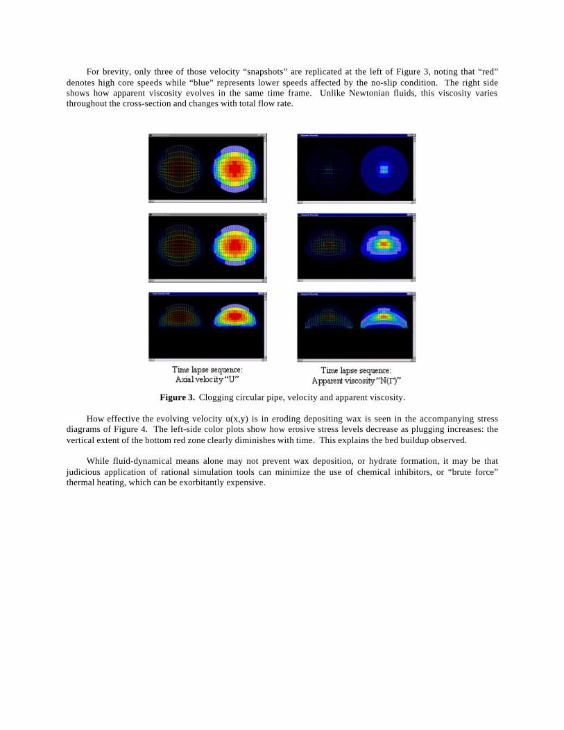
For brevity, only three of those velocity “snapshots” are replicated at the left of Figure 3, noting that “red”denotes high core speeds while “blue” represents lower speeds affected by the no-slip condition. The right sideshows how apparent viscosity evolves in the same time frame. Unlike Newtonian fluids, this viscosity variesthroughout the cross-section and changes with total flow rate.

Figure 3. Clogging circular pipe, velocity and apparent viscosity.

How effective the evolving velocity u(x,y) is in eroding depositing wax is seen in the accompanying stressdiagrams of Figure 4. The left-side color plots show how erosive stress levels decrease as plugging increases: thevertical extent of the bottom red zone clearly diminishes with time. This explains the bed buildup observed.

While fluid-dynamical means alone may not prevent wax deposition, or hydrate formation, it may be thatjudicious application of rational simulation tools can minimize the use of chemical inhibitors, or “brute force”thermal heating, which can be exorbitantly expensive.

Figure 4. Rectangular viscous stress components.

New Modeling Concepts

Most pipe flow practitioners are familiar with the concept behind “non-Newtonian” fluids. For ideal fluids likewater and air, doubling the pressure gradient will double the flow rate. Since most pressure drops are small anyway,pipeline modeling errors are not all that significant.

Figure 5. “Flow rate ‘Q’ versus pressure gradient” for various “n.”

The situation is different for fluids with complicated stress-strain relationships, e.g., power law fluids,Bingham plastics, and Herschel-Bulkley flows. Figure 5 shows how “flow rate versus pressure gradient linearity”rarely applies. In fact, the degree of nonlinearity depends on the pressure drop, plus details related to the geometry.

One quantity significant to pipeline design is “equilibrium radius.” Will a given pipeline clog or not? If therheological properties of the fluid and the mechanical yield properties of the debris lining are known, what is theradius where viscous stresses imparted by the flow exactly equal those needed to erode wax or hydrate coatings?

Initial Clean Pipe Final Equilibrium RadiusDebris Buildup

Figure 6. Debris buildup leading to clogged (but opened) pipe.

What is a “good” equilibrium radius? Obviously, one that is “zero” is undesirable; small radii are no better,since pumping requirements can be severe. The simple case of a pipe having a circular cross-section is shown inFigure 6. Theoretical equilibrium radii (in inches) obtained from an analytical model appear on the vertical axis inFigure 7.

Figure 7. Equilibrium radius depends on fluid rheology.

For the Bingham plastic assumed, numerical results show that high levels of yield stress (tau-y, in psi) andplastic viscosity (as Cp) efficiently “open up” the pipe to flow. For the flow rate used, inner “clog diameters”remain no less than, say, 5 inches. But that particular value is dependent on the production rate assumed and theyield stress of the pipe lining, and it will typically vary from rheology to rheology.

Closing Remarks

There are no clear answers to designing clog-free pipelines. But the possibility of reducing the frequency offlow obstructions using computational simulations exists, because rigorous modeling efficiently extrapolateslaboratory data to real world behavior encompassing broad parameter ranges.

In Part III, we examine “bundled pipeline” systems that heat the fluid internally, requiring coupled velocity andthermal modeling. While less attractive from a fabrication perspective, they do provide a flow alternative that ismore desirable. Advanced simulation approaches will be discussed, particularly with pipeline economics in mind.

References

Chin, W. C., “Modern Flow Assurance Methods, Part I: Clogged Pipelines, Wax Deposition, and Hydrate Plugs,”Offshore Magazine, September 2000.

Chin, W. C., Borehole Flow Modeling, Gulf Publishing, Houston, 1991.

Chin, W. C., Computational Rheology for Pipeline and Annular Flow, Reed Elsevier, 2001.

Reprinted from Offshore Magazine, November 2000

Modern Flow Assurance Methods, Part III:Coupled Velocity and Temperature Fields in Bundled Pipelines

by

Wilson C. Chin, Ph.D., M.I.T.

Introduction

Strong industry interest in deep subsea exploration and production has elevated the importance of “flowassurance modeling,” the study of fluid flow under less than ideal circumstances. In Parts I and II of this series, wehighlighted the role of modern computational methods in quantifying the delicate balance struck between nonlinearfluid rheology and the geometric complexity that arises from pipeline clogging (see References 1 and 2).

These articles described applications of the finite difference simulation methodology developed in Reference 3.In particular, we showed how “fluids-solids interaction models” extrapolated from laboratory observation can beused to support full-scale, dynamic models of unsteady wax deposition and hydrate plug formation in pipes.

Color graphics played a crucial “diagnostic” role in explaining why some pipes clogged and why others erodedaway growing debris beds. In these papers, not only was velocity distribution shown, with “red” indicating “fast,”and “blue” denoting “slow,” but all components of the viscous stress tensor were displayed as well. Regions of lowstress would suggest continual debris growth, while high stress domains would point to the possibility of “self-cleaning.”

We also demonstrated how analytical and numerical models can predict “equilibrium cross-sections,” in whichthe mechanical yield stresses of the wax or hydrate deposits adhering to pipe walls identically equal thehydrodynamic stresses imparted by the flowing fluid. This equilibrium indicator answers the most importantquestion confronting flow assurance specialists: “Does the pipeline clog, or does it not?”

Why Bundled Pipelines?

In subsea applications where pipelines reside in extreme cold, waxes will precipitate out of solution to formbeds, or perhaps, adhere azimuthally to the pipe wall, and hydrate crystals may aggregate to form immovable plugs.The erosive force imparted by the shearing action of the moving fluid may not be strong enough to assure smoothunimpeded flow. When this is so, expensive chemical remediation and external heating may be required.

In this series, we focus on the interaction between fluid-dynamical and thermal fields only. In the simplestphysical limit when free convection effects are negligible compared to forced convection, and flow occurs in theaxial direction only, the equations of motion take on a tractable form amenable to mathematical solution. Theproperties of such flows can be explained rather straightforwardly.

Pipelines are often warmed by carrying within them separate lines that increase temperature by internalheating. “Pipes within pipelines” are known as “bundled pipelines.” In the simplest case, a circular pipe mightcontain another pipe which houses hot, flowing fluid, isolated from the production flow; the inner pipe can, ofcourse, be electrically heated too, or mounted to the side. The exact source of heat is not germane to our analysis.

Mathematical Formulation

The engineering problem posed above yields simplifications. In the leading approximation, the temperaturefield T(x,y) satisfies Laplace’s equation, with high temperatures prescribed at the inner pipe and cold oceantemperatures assumed at the outer walls.

The amount of heating required would depend on the thermodynamic properties of wax and hydrateappearance. The solution leads to a thermal field that varies rapidly in the flow domain, now an annular and not apipe cross-section, that strongly affects momentum transport properties like viscosity.

More precisely, we must speak of “n,” “k,” and “yield stress,” if general Herschel-Bulkley models are used tocharacterize wax or hydrate slurries. Unlike the flows treated in References 1 and 2 where “n” and “k” are constant,the dependence “n(T),” for example, now means that “n{T(x,y)}” or “n(x,y)” is variable within the flow. Thesevariable properties must be used for velocity and shear rate calculations.

Fortunately, the temperature equation and the modified flow equation for annular velocity can be solved usingthe finite difference scheme developed for “simple annuli” described in Reference 1. Only minor changes arerequired, since both differential equations are similar. For details, the reader should consult Chapters 2, 5 and 6 ofReference 3. The same color graphics tools can also be modified to display both temperature and velocity. Finally,we ask, “How do typical solutions behave?”

Coupled Velocity and Thermal Fields

Figure 1 summarizes our simulation capabilities very nicely. The left figures show computed solutions forvelocity (top) and temperature (bottom) assuming a small inner heat pipe. “Red” denotes “fast” for velocities and“hot” for temperature. In contrast, “blue” represents “slow” and “cold.” The right figures display calculated resultsfor a hypothetical “large” inner pipe.

Figure 1. Coupled velocity and temperature fields.

Consider the left figures. The velocity solution shows rapid flow speeds in the wide part of the annulus, asexpected. For the temperature field, hot fluid surrounds the pipe, which rapidly adjusts to cold ambient conditions.In both cases, our use of advanced “boundary conforming, curvilinear” grids provides physical resolution in tightspaces as needed, and especially in the rapidly changing regions adjacent to the inner pipelines.

Of course, which flow is “better” in practice is not apparent from color plots or grid displays. In order todetermine economic viability, the volume throughput associated with the annular flow obviously enters. One mightspeculate that the higher the eccentricity, the better the production, since high eccentricities typically yield higherflow rates in many problems. But now, this may not be true, since our transport coefficients are variable.

Secondly, production economics is determined by heating costs. In the problem formulated above,temperatures are fixed at inner and outer boundaries. In order to maintain the assumed steady state, a nonzero heatflux is required along the entire length of the pipeline. This can add significantly to operating costs. But this maybe inexpensive, by comparison to a “no heating” scenario where the pipeline clogs, even just once.

Figure 2. Input properties definition screen.

Any credible economic model must address the factors introduced above, in addition to costs associated withconstruction and down-time. Just as important, any useful mathematical model must be easy to use, allowingconvenient input properties definition for the wax and hydrate slurries being modeled. This is crucial becauseengineers must consider numerous operating scenarios before optimal ones are identified.

Figure 2 shows the Windows-based “properties definition” screen used to define “n,” “k,” and “yield stress.”Consider, for example, the flow exponent “n.” The user enters a baseline value, say “1” for Newtonian flows orBingham plastics. Also, the gradient “dn/dT” is also supplied, where “T” again denotes temperature. Suchproperties are obtained from laboratory measurement. Once the geometry of the pipe bundle is specified, the“Simulate” command is “clicked” and solutions like those in Figure 1 appear within seconds.

Modeling “Real-World” Effects

In order to keep the discussion simple, we ignored the presence of time-varying debris bed heights andgrowing plug-like obstacles. Of course, the transient buildup and erosion development process must not beneglected, as noted in Part II, and Chapters 7 and 8 of Reference 3. Alterations in flow cross-section can affect theflow in unanticipated, serious, and subtle ways.

Figure 3. Velocity redistribution due to bed buildup.

In Figure 3, we give two examples of velocity fields encountered in our field studies. The picture at the leftillustrates a “typical” annular flow, that is, with expected high “red” velocities in the wide part. The one at the rightdescribes one possible flow pattern that arises with debris bed buildup.

The “red” zone displaces symmetrically in the lateral directions because the bottom annulus is dominated bythe “no-slip” condition. The initial red zone now bifurcates into two small domains, differently from what isexpected of “single pipe alone” flow. Because geometric similarity is completely lost, the new flow topologypossesses completely different “flow rate versus pressure gradient” properties from the former.

Mudcake growth proportional toDarcy pressure gradient

Wax growth proportional totemperature gradient

Figure 4. Azimuthal wax buildup around the pipe.

In Figure 3, we were concerned with beds that build preferentially at the bottom; however, “beds” may developfrom above too, for example, the result of buoyant, low-density wax in high density fluids. We did not showdeposition around the pipe, since the flow and ocean environment were assumed to be in thermal equilibrium.

Near the production well, equilibrium conditions may not apply. The flow may not be isothermal.Consequently, wax deposits about the entire inner surface, with a deposition rate that is proportional to the thermalgradient defined by pipe and ocean temperatures and the instantaneous layer thickness. Initially, debris buildup isquick; however, as the layer builds, the influence of the cold ocean is lessened and the growth rate decreases.

Another complicated model? Not quite. An interesting physical analogy can be drawn with mudcake buildupunder static filtration in a Darcy flow. In Figure 4, a “gray” mudcake is shown at the circular borehole face locatedin a cross-hatched Darcy formation, together with a “typically yellow” wax coating lining a circular pipe.

Here, filter-cake growth rate is proportional to the rate at which solid particles are left behind, that is, to thelocal pressure gradient. As the cake thickens, this gradient lessens and the rate of growth slows. The mathematicalanalogy between wax growth in hot pipelines and mudcake growth in boreholes, it is seen, is almost exact, andmodels developed for the latter can be used to simulate a “new” subsea phenomenon. Such deposition models arediscussed in Reference 4, which provides numerous models related to “formation invasion” in drilling.

Closing Remarks

In this final article of the three-part series on flow assurance modeling, we have shown how the general annularequation solver and color display algorithms introduced in Part I can be modified to solve for the coupled velocityand thermal fields typically encountered in bundled pipeline analysis.

Importantly, good production economics depends on just the right combination of high flow rate and low heatflux usage. Detailed numerical simulations are required, but because fast mapping and convergence accelerationmethods are now available, typical simulations - from input definition to final color output - can be completedwithin minutes.

Modern flow assurance analysis means more than studying rheological effects of wax and hydrate slurries incircular pipes. This is especially true because flow cross-sections are hardly circular: wax deposition can form deepbeds and hydrate aggregates can create immovable plugs. As shown in Parts II and III, these “difficult” flows canbe simulated conveniently. And, in general, computational methods are a “must,” because the competing effects ofnonlinear rheology, geometric complexity, and unsteady fluids and solids interaction, cannot be anticipatedbeforehand.

References

Chin, W. C., “Modern Flow Assurance Methods, Part I: Clogged Pipelines, Wax Deposition, and Hydrate Plugs,”Offshore Magazine, September 2000.

Chin, W. C., “Modern Flow Assurance Methods, Part II: Detailed Physical Properties and EngineeringApplication,” Offshore Magazine, October 2000.

Chin, W. C., Computational Rheology for Pipeline and Annular Flow, Reed Elsevier, 2001.

Chin, W. C., Formation Invasion, Gulf Publishing, Houston, 1995.

Acknowledgments

Several organizations have contributed to the overall work. In particular, Brown & Root Energy Services andHalliburton Energy Services are acknowledged for the development of solids deposition models; thanks are due toRaj Amin, Ron Morgan, Harry Smith, and Tin Win for their insights and encouragement. Advanced mappingresearch and convergence acceleration methods were funded by the United States Department of Energy underGrant No. DE-FG03-99ER82895. Also, the support of Gulf Publishing and the interest offered by PennWellPublishing are gratefully acknowledged.

Author’s Background

Wilson C. Chin earned his Ph.D. at M.I.T. and his M.Sc. from Cal Tech. He is presently affiliated with start-up company StrataMagnetic Software, LLC in Houston, Texas, a research organization focusing on computationalrheology, reservoir flow analysis, electromagnetic modeling, and software development. Mr. Chin has publishedover seventy related papers, obtained over forty oilfield patents, and authored five books on petroleum applications.He may be contacted by email at “wilsonchin@aol.com.”