Models for Real-Time Workload: A Survey

Martin Stigge and Wang Yi

Department of Information TechnologyUppsala University, Sweden

Email: {martin.stigge,yi}@it.uu.se

Abstract. This paper provides a survey on task models to characterize real-timeworkloads at different levels of abstraction for the design and analysis of real-timesystems. It covers the classic periodic and sporadic models by Liu and Layland etal., their extensions to describe recurring and branching structures as well as gen-eral graph- and automata-based models to allow modeling of complex structuressuch as mode switches, local loops and also global timing constraints. The focusis on the precise semantics of the various models and on the solutions and com-plexity results of the respective feasibilty and schedulability analysis problemsfor preemptable uniprocessors.

1 Introduction

Real-time systems are often implemented by a number of concurrent tasks sharinghardware resources, in particular the execution processors. The designer of such sys-tems need to construct workload models characterizing the resource requirements ofthe tasks. With a formal description of the workload, a resource scheduler may be de-signed and analyzed. The fundamental analysis problem to solve in the design processis to check (and thus to guarantee) the schedulability of the workload, i.e., whether thetiming constraints on the workload can be met if the scheduler is used. In addition, theworkload model may also be used to optimize the resource utilization as well as theaverage system performance.

In the past decades, workload models have been studied intensively in the theoryof real-time scheduling [20] and other contexts, for example performance analysis ofnetworked systems [19]. The research community of real-time systems has proposeda large number of models (often known as task models) allowing for the descriptionand analysis of real-time workloads at different levels of abstraction. One of the classicworks is the periodic task model due to Liu and Layland [40, 37, 38], where tasks gener-ate resource requests at strict periodic intervals. The periodic model was extended laterto the sporadic model [42, 9, 35] and multiframe models [44, 7] to describe non-regulararrival times of resource requests, and non-uniform resource requirements. In spite of alimited form of variation in release times and worst-case execution times, these repeti-tive models are highly deterministic. To allow for the description of recurring and non-deterministic behaviours, tree-like recurring models based on directed acyclic graphsare introduced [11, 10] and recently extended to the Digraph model based on arbitrarydirected graphs [50, 49] to allow for modeling of complex structures like mode switchesand local loops as well as global timing constraints on resource requests. With origin

from formal verification of timed systems, the model of task automata [28] was devel-oped in the late 90s. The essential idea is to use timed automata to describe the releasepatterns of tasks. Due to the expressiveness of timed automata, it turns out that all themodels above can be described using the automata-based model.

In addition to the expressiveness, a major concern in developing these models isthe complexity of their analysis. It is not surprising that the more expressive they are,the more difficult to analyze they tend to be. Indeed, the model of task automata is themost expressive model with the highest analysis complexity, which marks the border-line between decidability and undecidability for the schedulability analysis problem ofworkloads. On top of the operational models summarized above that capture the timedsequences of resource requests representing the system executions, alternative charac-terizations of workloads using functions on the time interval domain have also beenproposed, notably Demand Bound Function (DBF), Request Bound Function (RBF)and Real-Time Calculus (RTC) [55] that can be used to specify the accumulated work-load over a sliding time window. They have been further used as a mathematical toolfor the analysis of operational workload models.

Liu & Layland (3.1)(e,d = p)

sporadic (3.1)(e,d, p)

multiframe (3.2)(ei,d = p)

generalized multiframe (GMF) (3.3)(ei,di, pi)

recurring branching (RB) (4.2)(tree, p)

recurring RT (RRT) (4.3)(DAG, p)

non-cyclic GMF (3.4)(order arbitrary)

non-cyclic RRT (4.4)(DAG, pi)

Digraph (DRT) (4.5)(arbitrary graph)

Extended DRT (EDRT) (4.6)(graph + constraints)

efficient

Feas

ibili

tyte

st

difficult

low

Exp

ress

iven

ess

high

Strongly (co)NP-complete

Pseudo-Polynomial

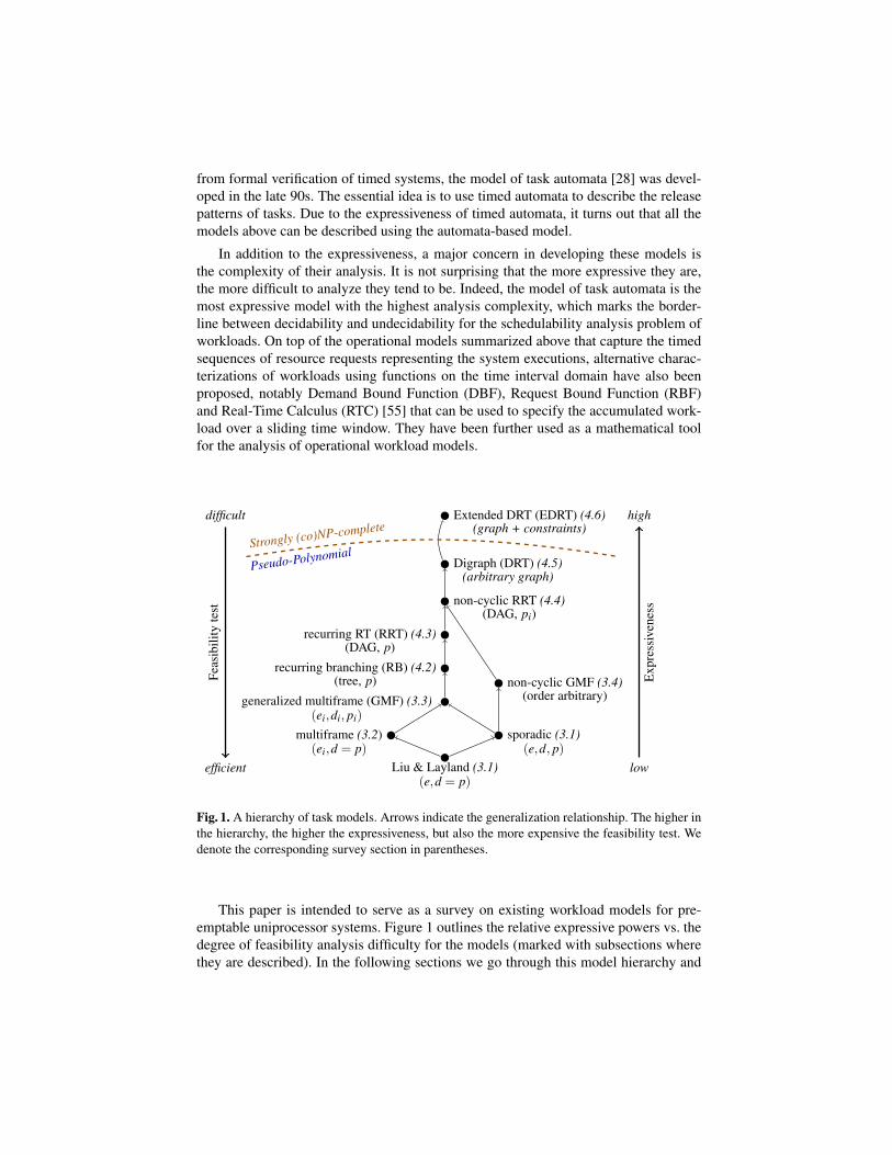
Fig. 1. A hierarchy of task models. Arrows indicate the generalization relationship. The higher inthe hierarchy, the higher the expressiveness, but also the more expensive the feasibility test. Wedenote the corresponding survey section in parentheses.

This paper is intended to serve as a survey on existing workload models for pre-emptable uniprocessor systems. Figure 1 outlines the relative expressive powers vs. thedegree of feasibility analysis difficulty for the models (marked with subsections wherethey are described). In the following sections we go through this model hierarchy and

provide a brief account for each of the well-developed models including the Real-TimeCalculus representing models on a higher level of abstraction.

2 Terminology

We first review some terminology used in the rest of this survey. The basic unit de-scribing workload is a job, characterized by a release time, a worst-case execution time(WCET) and a deadline. The higher-level structures which generate (potentially infi-nite) sequences of jobs are tasks. The time interval between the release time and thedeadline of a job is called its scheduling window. The time interval between the releasetime of a job and the earliest release time of its succeeding job from the same task is itsexclusion window.

A task system typically contains a set of tasks that at runtime generate sequencesof jobs concurrently and a scheduler decides at each point in time which of the pend-ing jobs to execute. We distinguish between two important classes of schedulers onpreemptable uniprocessor systems:

Static priority schedulers. Tasks are ordered by priority. All jobs generated by a taskof higher priority get precedence over jobs generated by tasks of lower priority.

Dynamic priority schedulers. Tasks are not ordered a priori; at runtime, the schedulermay choose freely which of the pending jobs to execute.

Given suitable descriptions of a workload model and a scheduler, one of the importantquestions is whether all jobs that could ever be generated will meet their deadline con-straints, in which case we call the workload schedulable. This is determined in a formalschedulability test which can be:

Sufficient if it is failed by all non-schedulable task sets,Necessary, if it is satisfied by all schedulable task sets, orPrecise or exact if it is both sufficient and necessary.

More precisely, if a task set satisfies a sufficient test, it is schedulable and if it failsa necessary test, it is non-schedulable. Workload that is schedulable with some effec-tive scheduler is called feasible, determined by a feasibility test that can also be eithersufficient, necessary or both.

3 Repetitive Models: From Liu and Layland Tasks to GMF

In this section, we show the development of task systems from the periodic task modelto different variants of the Multiframe model, including techniques for their analysis.

3.1 Periodic and Sporadic Tasks

The first task model with periodic tasks was introduced 1973 by Liu and Layland [40].Each periodic task T = (P,E) in a task set τ is characterized by a pair of two integers:period P and WCET E. It generates an infinite sequence ρ = (J1,J2, . . .) of jobs Ji =

(ri,ei,di) with release time ri, execution time ei and deadline di such that ri+1 = di =ri + P and ei 6 E. This means that jobs are released periodically and have implicitdeadlines at the release times of the next job.

A relaxation of this model is to allow jobs to be released at later time points, aslong as at least P time units pass between adjacent job releases of the same task. This iscalled the sporadic task model, introduced by Mok in [42]. Another generalization is toadd an explicit deadline D as a third integer to the task definition T = (P,E,D), leadingto di = ri +D for all generated jobs. If D 6 P for all tasks T ∈ τ then we say that τ hasconstrained deadlines, otherwise it has arbitrary deadlines.

This model has been the basis for many results throughout the years. Liu and Lay-land give in [40] a simple feasibility test for implicit deadline tasks: defining the uti-lization U(τ) of a task set τ as U(τ) := ∑Ti∈τ Ei/Pi, a task set is uniprocessor feasibleif and only if U(τ) 6 1. As in later work, proofs of feasibility are often connected tothe Earliest Deadline First (EDF) scheduling algorithm, which uses dynamic prioritiesand has been shown to be optimal for a large class of workload models on uniprocessorplatforms. Because of its optimality, EDF schedulability is equivalent to feasibility.

Demand bound function. For the case of explicit deadlines, Baruah et al. [9] introduceda concept that was later called the demand bound function: for each interval size tand task T , dbf T (t) is the maximum accumulated worst-case execution time of jobsgenerated by T in any interval of size t. More specifically, it counts all jobs that havetheir full scheduling window inside the interval, i.e., release time and deadline. Thedemand bound function dbf (t) of the whole system has the property that a task systemis feasible if and only if

∀t.dbf (t)6 t. (1)

This condition is a valid test for a very general class of workload models and is ofgreat use in later parts of this survey. It holds for all models generating sequences ofindependent jobs. A proof can be found in [7].

Focussing on sporadic tasks, Baruah et al. show in [9] that dbf (t) can be computedwith

dbf (t) = ∑Ti∈τ

Ei ·max{

0,⌊

t−Di

Pi

⌋+1}. (2)

Using this they prove that the feasibility problem is in coNP. Recently it has been shownby Eisenbrand and Rothvoß [25] that the problem is indeed (weakly) coNP-hard forsystems with constrained deadlines.

Another contribution of Baruah et al. in [9] was to show that for the case of U(τ)< cfor some constant c, there is a pseudo-polynomial solution of the schedulability prob-lem, by testing Condition (1) for a pseudo-polynomial number of values. The existenceof such a constant bound (however close to 1) is a common assumption when approach-ing this problem since excluding utilizations very close to 1 only rules out very fewactual systems.

Static priorities. For static priority schedulers, Liu and Layland show already in [40]that the rate-monotonic priority assignment for implicit deadline tasks is optimal, i.e.,tasks with shorter periods have higher priorities. They further give an elegant sufficient

schedulability condition by proving that a task set τ with n tasks is schedulable with astatic priority scheduler under rate-monotonic priority ordering if

U(τ)6 n · (21/n−1). (3)

For sporadic task systems with explicit deadlines, the response time analysis techniquehas been developed. It is based on a scenario in which all tasks release jobs at the sametime instant with all following jobs being released as early as permitted. This maximizesthe response time Ri of the task in question, which is why the scenario is often called thecritical instant. It is shown by Joseph and Pandya [33] and independently by Audsleyet al. [3] that Ri is the smallest positive solution of the recurrence relation

R = Ei +∑j<i

⌈RPj

⌉·E j, (4)

assuming that the tasks are in order of descending priority. This is based on the obser-vation that the interference from a higher priority task Tj to Ti during a time interval ofsize R can be computed by counting the number of jobs Tj can release as

⌈R/Pj

⌉and

multiplying that with their worst-case duration E j. Together with Ti’s own WCET Ei,the response time is derived. Solving Equation (4) leads directly to a pseudo-polynomialschedulability test. Eisenbrand and Rothvoß show in [24] that the problem of computingRi is indeed NP-hard.

3.2 The Multiframe Model

The first extension of the periodic and sporadic paradigm for jobs of different types, tobe generated from the same task was introduced by Mok and Chen in [44]. The motiva-tion is as follows. Assume a workload which is fundamentally periodic but it is knownthat every k-th job of this task is extra long. As an example, Mok and Chen describean MPEG video codec that uses different types of video frames. Video frames arriveperiodically, but frames of large size and thus large decoding complexity are processedonly once in a while. The sporadic task model would need to account for this in theWCET of all jobs, which is certainly a significant overapproximation. Systems that areclearly schedulable in practice would fail standard schedulability tests for the sporadictask model. Thus, in scenarios like this where most jobs are close to an average compu-tation time which is significantly exceeded only in well-known periodically recurringsituations, a more precise modeling formalism is needed.

To solve this problem, Mok and Chen introduce in [44] the Multiframe model. Amultiframe task T is described as a pair (P,E) much like the basic sporadic modelwith implicit deadlines, except that E = (E0, . . . ,Ek−1) is a vector of different executiontimes, describing the WCET of k potentially different frames.

Semantics. As before, let ρ = (J1,J2, . . .) be a job sequence with job parameters Ji =(ri,ei,di) of release time ri, execution time ei and deadline di. For ρ to be generated bya multiframe task T with k frames, it has to hold that ei 6 E(a+i) mod k for some offseta, i.e., the worst-case execution times cycle through the list specified by vector E. Theother job parameters ri and di behave as before for sporadic implicit-deadline tasks, i.e.,ri+1 > ri +P = di. We show an example in Figure 2.

Frame 0 Frame 1 Frame 2 Frame 3 Frame 0

t

Fig. 2. Example for a Multiframe task T = (P,E) with P = 4 and E = (3,1,2,1). Note that dead-lines are implicit.

Schedulability Analysis. Mok and Chen provide in [44] a schedulability analysis forstatic priority scheduling. They provide a generalization of Equation (3) by showingthat a task set τ is schedulable with a static priority scheduler under rate-monotonicpriority ordering if

U(τ)6 r ·n ·((1+1/r)1/n−1

). (5)

The value r in this test is the minimal ratio between the largest WCET Ei in a task andits successor E(i+1) mod k. Note that the classic test for periodic tasks in Equation (3) isa special case of (5) with r = 1.

The proof for this condition is done by carefully observing that for a class of Multi-frame tasks called accumulatively monotonic (AM), there is a critical instant that can beused to derive the condition (and further even for a precise test in pseudo-polynomialtime by simulating the critical instant). In short, AM means that there is a frame in eachtask such that all sequences starting from this frame always have a cumulative execu-tion demand at least as high as equally long sequences starting from any other frame.After showing (5) for AM tasks the authors prove that each task can be transformed intoan AM task which is equivalent in terms of schedulability. The transformation is via amodel called General Tasks from [43] which is an extension of Multiframe tasks to aninfinite number of frames and therefore of mainly theoretical interest.

Refined sufficient tests have been developed [32, 57, 41] with less pessimism thanthe test using the utilization bound in (5). They generally also allow certain tasks ofhigher utilization than those passing the above test to be classified as schedulable. Aprecise test of exponential complexity is presented in [58] based on response time anal-ysis as a generalization of (4). The authors also include results for models with jitterand blocking.

3.3 Generalized Multiframe Tasks

In the Multiframe model, all frames still have the same period and implicit deadline.Baruah et al. generalize this further in [7] by introducing the Generalized Multiframe(GMF) task model. A GMF task T = (P,E,D) with k frames consists of three vectors:

P = (P0, . . . ,Pk−1) for minimum inter-release separations,E = (E0, . . . ,Ek−1) for worst-case execution times, andD = (D0, . . . ,Dk−1) for relative deadlines.

For unambiguous notation we write PTi , ET

i and DTi for components of these three

vectors in situations where it is not clear from the context which task T they belong to.

Semantics. As a generalization of the Multiframe model, each job Ji = (ri,ei,di) in ajob sequence ρ = (J1,J2, . . .) generated by a GMF task T needs to correspond to a frameand the corresponding values in all three vectors. Specifically, we have for some offseta that:

1. ri+1 > ri +P(a+i) mod k2. ei 6 E(a+i) mod k3. di = ri +D(a+i) mod k

An example is shown in Figure 3.

Frame 0 Frame 1 Frame 2 Frame 0 Frame 1

t

Fig. 3. Example for a GMF task T = (P,E,D) with P = (5,3,4), E = (3,1,2) and D = (3,2,3).

Feasibility Analysis. Baruah et al. give in [7] a feasibility analysis method based on thedemand bound function. The different frames make it difficult to develop a closed-formexpression like (2) for sporadic tasks since there is in general no unique critical instantfor GMF tasks. Instead, the described method (which we sketch here with slightly ad-justed notation and terminology) creates a list of pairs 〈e,d〉 of workload e and sometime interval length d which are called demand pairs in later work [50]. Each demandpair 〈e,d〉 describes that a task T can create e time units of execution time demandduring an interval of length d. From this information it can be derived that dbf T (d)> esince the demand bound function dbf T (d) is the maximal execution demand possibleduring any interval of that size.

In order to derive all relevant demand pairs for a GMF task, Baruah et al. first intro-duce a property called localized Monotonic Absolute Deadlines (l-MAD). Intuitively, itmeans that two jobs from the same task that have been released in some order will alsohave their (absolute) deadlines in the same order. Formally, this is can be expressed asDi 6 Pi +D(i+1) mod k, which is more general than the classical notion of constraineddeadlines, i.e., Di 6 Pi, but still sufficient for the analysis. We assume this property forthe rest of this section.

As preparation, the method from [7] creates a sorted list DP of demand pairs 〈e,d〉for all i and j each ranging from 0 to k−1 with

e =i+ j

∑m=i

Em mod k, d =

(i+ j−1

∑m=i

Pm mod k

)+D(i+ j) mod k. (6)

For a particular pair of i and j, this computes in e the accumulated execution timeof a job sequence with jobs corresponding to frames i, . . . ,(i + j) mod k. The value

of d is the time from first release to last deadline of such a job sequence. With allthese created demand pairs, and using shorthand notation Psum := ∑

k−1i=0 Pi, Esum :=

∑k−1i=0 Ei and Dmin := mink−1

i=0 Di, the function dbf T (t) can be computed with

dbf T (t)=

0 if t < Dmin,

max{e | 〈e,d〉 ∈ DP with d 6 t} if t ∈ [Dmin,Psum +Dmin),⌊t−Dmin

Psum

⌋Esum +dbf T

(Dmin +(t−Dmin) mod Psum

)if t > Psum +Dmin.

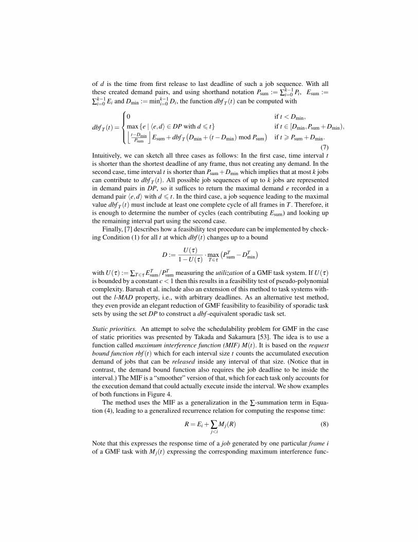
(7)Intuitively, we can sketch all three cases as follows: In the first case, time interval tis shorter than the shortest deadline of any frame, thus not creating any demand. In thesecond case, time interval t is shorter than Psum+Dmin which implies that at most k jobscan contribute to dbf T (t). All possible job sequences of up to k jobs are representedin demand pairs in DP, so it suffices to return the maximal demand e recorded in ademand pair 〈e,d〉 with d 6 t. In the third case, a job sequence leading to the maximalvalue dbf T (t) must include at least one complete cycle of all frames in T . Therefore, itis enough to determine the number of cycles (each contributing Esum) and looking upthe remaining interval part using the second case.

Finally, [7] describes how a feasibility test procedure can be implemented by check-ing Condition (1) for all t at which dbf (t) changes up to a bound

D :=U(τ)

1−U(τ)·max

T∈τ

(PT

sum−DTmin)

with U(τ) := ∑T∈τ ETsum/PT

sum measuring the utilization of a GMF task system. If U(τ)is bounded by a constant c< 1 then this results in a feasibility test of pseudo-polynomialcomplexity. Baruah et al. include also an extension of this method to task systems with-out the l-MAD property, i.e., with arbitrary deadlines. As an alternative test method,they even provide an elegant reduction of GMF feasibility to feasibility of sporadic tasksets by using the set DP to construct a dbf -equivalent sporadic task set.

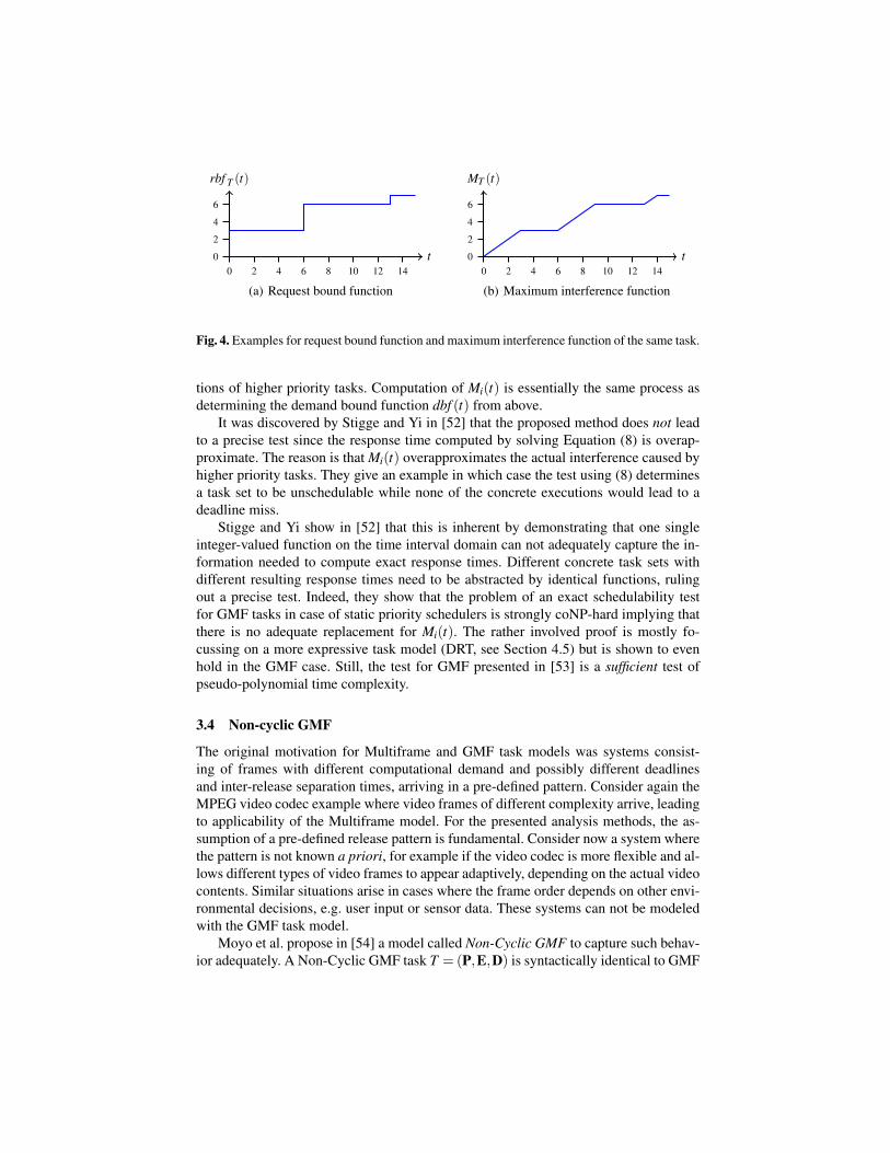
Static priorities. An attempt to solve the schedulability problem for GMF in the caseof static priorities was presented by Takada and Sakamura [53]. The idea is to use afunction called maximum interference function (MIF) M(t). It is based on the requestbound function rbf (t) which for each interval size t counts the accumulated executiondemand of jobs that can be released inside any interval of that size. (Notice that incontrast, the demand bound function also requires the job deadline to be inside theinterval.) The MIF is a “smoother” version of that, which for each task only accounts forthe execution demand that could actually execute inside the interval. We show examplesof both functions in Figure 4.

The method uses the MIF as a generalization in the ∑-summation term in Equa-tion (4), leading to a generalized recurrence relation for computing the response time:

R = Ei +∑j<i

M j(R) (8)

Note that this expresses the response time of a job generated by one particular frame iof a GMF task with M j(t) expressing the corresponding maximum interference func-

t0 2 4 6 8 10 12 14

rbf T (t)

0

2

4

6

(a) Request bound function

t0 2 4 6 8 10 12 14

MT (t)

0

2

4

6

(b) Maximum interference function

Fig. 4. Examples for request bound function and maximum interference function of the same task.

tions of higher priority tasks. Computation of Mi(t) is essentially the same process asdetermining the demand bound function dbf (t) from above.

It was discovered by Stigge and Yi in [52] that the proposed method does not leadto a precise test since the response time computed by solving Equation (8) is overap-proximate. The reason is that Mi(t) overapproximates the actual interference caused byhigher priority tasks. They give an example in which case the test using (8) determinesa task set to be unschedulable while none of the concrete executions would lead to adeadline miss.

Stigge and Yi show in [52] that this is inherent by demonstrating that one singleinteger-valued function on the time interval domain can not adequately capture the in-formation needed to compute exact response times. Different concrete task sets withdifferent resulting response times need to be abstracted by identical functions, rulingout a precise test. Indeed, they show that the problem of an exact schedulability testfor GMF tasks in case of static priority schedulers is strongly coNP-hard implying thatthere is no adequate replacement for Mi(t). The rather involved proof is mostly fo-cussing on a more expressive task model (DRT, see Section 4.5) but is shown to evenhold in the GMF case. Still, the test for GMF presented in [53] is a sufficient test ofpseudo-polynomial time complexity.

3.4 Non-cyclic GMF

The original motivation for Multiframe and GMF task models was systems consist-ing of frames with different computational demand and possibly different deadlinesand inter-release separation times, arriving in a pre-defined pattern. Consider again theMPEG video codec example where video frames of different complexity arrive, leadingto applicability of the Multiframe model. For the presented analysis methods, the as-sumption of a pre-defined release pattern is fundamental. Consider now a system wherethe pattern is not known a priori, for example if the video codec is more flexible and al-lows different types of video frames to appear adaptively, depending on the actual videocontents. Similar situations arise in cases where the frame order depends on other envi-ronmental decisions, e.g. user input or sensor data. These systems can not be modeledwith the GMF task model.

Moyo et al. propose in [54] a model called Non-Cyclic GMF to capture such behav-ior adequately. A Non-Cyclic GMF task T = (P,E,D) is syntactically identical to GMF

task from Section 3.3, but with non-cyclic semantics. In order to define the semanticsformally, let φ : N→ {0, . . . ,k−1} be a function choosing frame φ(i) for the i-th jobof a job sequence. Having φ , each job Ji = (ri,ei,di) in a job sequence ρ = (J1,J2, . . .)generated by a non-cyclic GMF task T needs to correspond to frame φ(i) and the cor-responding values in all three vectors:

1. ri+1 > ri +Pφ(i)2. ei 6 Eφ(i)3. di = ri +Dφ(i)

This contains cyclic GMF job sequences as the special case where φ(i) = (a+ i) mod kfor some offset a. An example of non-cyclic GMF semantics is shown in Figure 5.

Frame 0 Frame 2 Frame 1 Frame 1 Frame 1

t

Fig. 5. Non-cyclic semantics of the GMF example Figure 3

For analysing non-cyclic GMF models, Moyo et al give in [54] a simple density-based sufficient feasibility test. Defining D(T ) := maxi CT

i /DTi as the densitiy of a task

T , a task set τ is schedulable if ∑T∈τ D(T ) 6 1. This generalizes a similar test for thesporadic task model with explicit deadlines. In addition to this test, [54] also includesan exact feasibility test based on efficient systematic simulation.

A different exact feasibility test is presented in [13] for constrained deadlines usingthe demand bound function condition (1). A dynamic programming approach is usedto compute demand pairs (see Section 3.3) based on the observation that dbf T (t) canbe computed for larger and larger t reusing earlier values. More specifically, a functionAT (t) is defined which denotes for an interval size t the accumulated execution demandof any job sequence where jobs have their full exclusion window inside the interval. Itis shown that AT (t) for t > 0 can be computed by assuming that some frame i was thelast one in a job sequence contributing a value to AT (t). In that case, the function valuefor the remaining job sequence is added to the execution time of that specific frame i.Since frame i is not known a priori, the computation has to take the maximum over allpossibilities. Formally,

AT (t) = maxi

{AT (t−PT

i )+ETi | PT

i 6 t}. (9)

Using this, dbf T (t) can be computed via the same approach by maximising over all pos-sibilities of the last job in a sequence contributing to dbf T (t). It uses that the executiondemand of the remaining job sequence is represented by function AT (t), leading to

dbf T (t) = maxi

{AT (t−DT

i )+ETi | DT

i 6 t}. (10)

This leads to a pseudo-polynomial time bound for the feasibility test if U(τ) is boundedby a constant, since dbf (t) > t implies t <

(∑T,i ET

i)/(1−U(τ)) which is pseudo-

polynomial in this case.The same article also proves that evaluating the demand bound function is a (weakly)

NP-hard problem. More precisely: Given a non-cyclic GMF task T and two integers tand B it is coNP-hard to determine whether dbf T (t) 6 B. The proof is via a ratherstraight-forward reduction from the Integer Knapsack problem. Thus, a polynomial al-gorithm for computing dbf (t) is unlikely to exist.

Static priorities. A recent result by Berten and Goossens [18] proposes a sufficientschedulability test for static priorities. It is based on the request bound function similarto [53] and its efficient computation. Similar to the approach in [53] the function isinherently overapproximate and the test is of pseudo-polynomial time complexity.

4 Graph-oriented Models

The more expressive workload models become, the more complicated structures arenecessary to describe them. In this section we turn to models based on different classesof directed graphs. We start by recasting the definition of GMF in terms of a graphrelease structure.

4.1 Revisiting GMF

Recall the Generalized Multiframe task model from Section 3.3. A GMF task T =(P,E,D) consists of three vectors for minimum inter-release separation times, worst-case execution times and relative deadlines of k frames. The same structure can beimagined as a directed cycle graph1 G = (V,E) in which each vertex v ∈ V representsthe release of a job and each edge (v,v′) ∈ E represents the corresponding inter-releaseseparation. A vertex v is associated with a pair 〈e(v),d(v)〉 for WCET and deadlineparameters of the represented jobs. An edge (u,v) is associated with a value p(u,v) forthe inter-release separation time.

The cyclic graph structure directly visualizes the cyclic semantics of GMF. In con-trast, non-cyclic GMF can be represented by a complete digraph. Figure 6 illustratesthe different ways of representing a GMF task with both semantics.

4.2 Recurring Branching Tasks

A first generalization to the GMF model was presented in [11]. It is based on the obser-vation that real-time code may include branches that influence the pattern in which jobsare released. As the result of some branch, a sequence of jobs may be released whichmay differ from the sequence released in a different branch. In a schedulability analysis,none of the branches may be universally worse than the others since that may dependon the situation, e.g., which tasks are being scheduled together with the branching one.

1 A cycle graph is a graph consisting of one single cycle, i.e., one closed chain.

T = (P,E,D)

P = (10,8,3,5,5)E = (1,2,3,1,1)

D = (10,7,7,9,8)

(a) T as vectors

v1〈1,10〉

v2

〈2,7〉

v3

〈3,7〉

v4

〈1,9〉 v5

〈1,8〉

108

3

5 5

(b) T as cycle graph

v1

v2

v3

v4

v5

(c) T as complete graph

Fig. 6. Different ways of representing a GMF task T . The vector-representation in 6(a) fromSection 3.3 does by itself not imply cyclic or non-cyclic semantics. This is more clear with graphsin 6(b) and 6(c). Note that we omit vertex and edge labels in 6(c) for clarity.

Thus, all branches need to be modeled explicitly and a proper representation is needed,different from the GMF release structure.

A natural way of representing branching code is a tree. Indeed, the model proposedin [11] is a tree representing job releases and their minimum inter-release separationtimes. We show an example in Figure 7(a). Formally, a Recurring Branching (RB) taskT is a directed tree G(T ) = (V,E) in which, as in Section 4.1, each vertex v ∈ V rep-resents a type of job to be released and each edge (u,v) ∈ E the minimum inter-releaseseparation times. They have labels 〈e(v),d(v)〉 and p(u,v) as before. In addition to thetree, each leaf u has a separation time p(u,vroot) to the root vertex vroot in order to modelthat the behavior recurs after each traversal of the tree.

u1

〈3,4〉u2

〈5,8〉 u3

〈1,15〉

u4

〈1,16〉u5

〈1,17〉

10

11

11

12

20

20

29

(a) RB task

u1

〈3,4〉u2

〈5,8〉 u3

〈1,15〉

u4

〈1,16〉u5

〈1,17〉

u6

〈3,6〉

10

11

11

12 4

31

20

25

P = 100

(b) RRT task

u1

〈3,4〉u2

〈5,8〉 u3

〈1,15〉

u4

〈1,16〉u5

〈1,17〉

10

11

11

12 4

31

20

30

(c) Non-cyclic RRT task

Fig. 7. Examples for RB, RRT and non-cyclic RRT task models

In order to simplify the feasibility analysis, the model is syntactically restricted inthe following way. For each path π = (v0, . . . ,vl) of length l from the root v0 = vrootto a leaf vl , its duration when going back to the root must be the same, i.e., the valueP := ∑

l−1i=0 p(vi,vi+1)+ p(vl ,vroot) must be independent of π . We call P the period of T .

Note that this is a generalization of GMF since GMF can be expressed as a linear tree.

Semantics. A job sequence ρ = (J1,J2, . . .) is generated by an RB task T if it corre-sponds to a path π through G(T ) in the following way. Path π starts at some vertex v1in G(T ), follows the edges to a leaf, then starts again at the root vertex, traverses G(T )again in a possibly different way, etc. (Very short π may of course never reach a leaf.)The correspondence between ρ and π means that for all Ji = (ri,ei,di), we have:

1. ri+1 > ri + p(vi,vi+1),2. ei 6 e(vi),3. di = ri +d(vi).

Feasibility Analysis. The analysis presented in [11] is based on the concept of demandpairs as described before. We sketch the method from [11] in a slightly adjusted manner.First, a set DP0 is created consisting of all demand pairs corresponding to paths notcontaining both a leaf and a following root vertex. This is straight forward since foreach pair of vertices (u,v) in G(T ) connected by a directed path π , this connecting pathis unique. Thus, a demand pair 〈e,d〉 can be created by enumerating all vertex pairs(u,v) and computing for their connecting path π = (v0, . . . ,vl) the values

e :=l

∑i=0

e(vi), d :=l−1

∑i=0

p(vi,vi+1)+d(vl). (11)

Second, all paths π which do contain both a leaf and a following root vertex can becut into three subpaths πhead, πmiddle and πtail:

π = (v, . . . ,vl︸ ︷︷ ︸πhead

,vroot,v′, . . . ,v′l ,vroot,v′′, . . . ,v′′l︸ ︷︷ ︸πmiddle

,vroot,v′′′, . . . ,v′′′′)︸ ︷︷ ︸πtail

We use vl , v′l , etc. for arbitrary leaf nodes. The first part πhead is the prefix of π up toand including the first leaf in π . The second part πmiddle is the middle part starting withvroot and ending in the last leaf which π visits. Note that πmiddle may traverse the treeseveral times. The third part πtail starts with the last occurrence of vroot in π . For eachof the three parts, a data structure is created so that demand pairs for a full path π canbe assembled easily.

For representing πhead, a set UPleaf is created. For all paths πhead = (v0, . . . ,vl) thatend in a leaf it contains a pair 〈e, p〉 with

e :=l

∑i=0

e(vi), p :=l−1

∑i=0

p(vi,vi+1)+ p(vl ,vroot). (12)

For representing πmiddle, the maximal accumulated execution demand emax of any pathcompletely traversing the tree is computed. Note that all paths from the root to a leaf

have the same sum of inter-release separation times and this sum is the period P ofT . Finally, for representing πtail, a set DProot is computed as a subset of DP0 onlyconsidering paths starting at vroot.

Using these data structures, dbf T (t) can be computed easily. If t 6 P, then a job se-quence contributing to dbf T (t) either corresponds to a demand pair in DP0 (not passingvroot) or is represented by items from UPleaf and DProot (since it is passing vroot exactlyonce):

F1(t) = max{e | 〈e,d〉 ∈ DP0 with d 6 t} (13)

F2(t) = max{

e1 + e2 | 〈e1, p〉 ∈ UPleaf ∧〈e2,d〉 ∈ DProot ∧ p+d 6 t}

(14)dbf T (t) = max{F1(t), F2(t)} if t 6 P (15)

In case t > P, such a job sequence must pass through vroot and traverses the tree com-pletely for either bt/Pc or bt/Pc− 1 times. For the parts that can be represented byπhead and πtail of the corresponding path π , we can use dbf T (t) from Equation (15),since πhead concatenated with πtail correspond to a job sequence without a completetree traversal. Putting it together for t > P:

F3(t) =⌊ t

P

⌋· emax +dbf T (t mod P) (16)

F4(t) =⌊

t−PP

⌋· emax +dbf T ((t−P) mod P) if t > P, 0 otherwise (17)

dbf T (t) = max{F3(t), F4(t)} if t > P (18)

Finally, in order to do the feasibility test, i.e., verify Condition (1), the demandbound function dbf (t) = ∑T dbf T (t) is computed for all t up to a bound D derived in asimilar way as for GMF in Section 3.3.

4.3 Recurring Real-Time Tasks (RRT) – DAG structures

In typical branching code, the control flow is joined again after the branches are com-pleted. Thus, no matter which branch is taken, the part after the join is common to bothchoices. In the light of a tree release structure as in the RB task model above, this meansthat many vertices in the tree may actually represent the same types of jobs to be re-leased, or even whole subtrees are equal. In order to make use of these redundancies,Baruah proposes in [10] to use a directed acyclic graph (DAG) instead of a tree. Theimpact is mostly efficiency: each DAG can be unrolled into a tree, but that comes at thecost of potentially exponential growth of the graph.

A Recurring Real-Time Task (RRT) T is a directed acyclic graph G(T ). The defini-tion is very similar to RB tasks in the previous section, we only point out the differences.It is assumed that G(T ) contains one unique source vertex (corresponding to vroot in anRB task) and further one unique sink vertex (corresponding to leafs in a tree). An RRTtask has an explicitly defined period parameter P that constrains the minimum timebetween two releases of jobs represented by the source vertex. An RRT behaves justlike an RB task by following paths through the DAG. We skip the details and give anexample of an RRT task in Figure 7(b).

Feasibility Analysis. Because of its close relation to RB tasks, the feasibility analysismethod presented in [10] is very similar to the method presented above for RB tasksand we skip the details. However, the adapted method has exponential complexity sinceit enumerates paths explicitly.

Chakraborty et al. present a more efficient method in [21] based on a dynamic pro-gramming approach, leading back to pseudo-polynomial complexity. Instead of enu-merating all pairs of vertices (u,v) in the DAG, the graph is traversed in a breadth-firstmanner. The critical observation is that all demand pairs representing a path ending inany particular vertex v can be computed from those for paths ending in all parent ver-tices. It is not necessary to have precise information about which the actual paths arethat the demand pairs represent. Even though Chakraborty et al. consider a limited vari-ant of the model in which paths traverse the DAG only once, the ideas can be appliedin general to the full RRT model.

The feasibility problem is further shown to be NP-hard in [21] via a reduction fromthe Knapsack problem and the authors give a fully polynomial time approximationscheme. For the special case where all vertices have equal WCET annotations, theyshow a polynomial time solution, similar to the dynamic programming technique above.

Static Priorities. A sufficient test for schedulability of an RRT task set with static pri-orities is presented in [12]. It is shown that, up to a polynomial factor, the priorityassignment problem in which a priority order has to be found is equivalent to the pri-ority testing problem where a task set with a given priority order is to be tested forschedulability. At the core of both is the test whether a given task T ∈ τ will meet itsdeadlines if it has the lowest priority of all tasks in τ (whose relative priority order doesnot matter). In that case T is called lowest-priority feasible.

The proposed solution gives a condition involving both the demand bound functiondbf T (t) and the request bound function rbf T (t). It is shown that a task T is lowest-priority feasible if

∀t. ∃t ′ 6 t. t ′ > dbf T (t)+ ∑T ′∈τ\{T}

rbf T ′(t′). (19)

It is shown that rbf T (t) can be computed with just a minor modification to the com-putation procedure of dbf T (t) and that Condition (19) only needs to be checked for abounded testing set of t, similar to the bound D introduced in checking Condition (1) infeasibility tests. For each t, checking the existence of a t ′ 6 t is essentially identical toan iterative procedure of solving the recurrence relation in Equation (8) of which (19)is a generalization.

A tighter and more efficient test is shown in [21] based on a smoother variant of therequest bound function, denoted rbf ′T (t). Using this, a task T is lowest-priority feasibleif

∀v ∈ G(T ). ∃t ′ 6 d(v). t ′ > e(v)+ ∑T ′∈τ\{T}

rbf ′T ′(t′). (20)

This test is a more direct and tighter generalization of the sufficient test (8) for GMFtasks.

4.4 Non-cyclic RRT

A further generalization of RRT is non-cyclic RRT2 [14] where the assumption of onesingle sink vertex is removed. Specifically, a non-cyclic RRT task T is a DAG G(T ) withvertex and edge labels as before that has a unique source vertex vsource. Additionally,for every sink vertex v, there is a value p(v,vsource) as before. We give an example inFigure 7(c). Note that a non-cyclic RRT task does not have a general period parameter,i.e., paths through G(T ) visiting vsource repeatedly may do so in differing time intervalswhen doing so through different sinks.

Feasibility Analysis. The analysis technique presented in [14] is similar to the onesof RB and RRT. The author uses the dynamic programming technique from [21] tocompute demand pairs inside the DAG in order to keep pseudo-polynomial complexityand assumes a partition of paths π into πhead, πmiddle and πtail as before. The differencehere is that paths traversing G(T ) completely from vsource to a sink may have differentlengths, i.e., πmiddle is not necessarily a multiple of some period P. Thus, the expressionsfor partial dbf T (t) computation in (16) and (17) can’t just assume a fixed length P anda fixed computation time emax. The idea to solve this is to first use the technique from[21] to compute demand pairs for full DAG traversals. These can then be interpretedas frames with a length and an execution time requirement, which can be concatenatedto achieve a certain interval length, like a very big non-cyclic GMF task. Similar to (9)for solving non-cyclic GMF feasibility, all possible paths going from source to a sinkcan be represented in a function AT (t) that expresses for each t the amount of executiondemand these special paths may create during intervals of length t. Similar to (10), thisfunction is integrated into (16) and (17), resulting in an efficient procedure.

The procedure is generalized in the following section which generalizes and unifiesall feasibility tests presented so far.

4.5 Digraph Real-Time Tasks

Stigge et al. observe in [50] that the non-cyclic RRT model can be generalized to anydirected graph. They introduce the Digraph Real-Time (DRT) task model and describea feasibility test of pseudo-polynomial complexity for task systems with utilizationbounded by a constant. A DRT task T is described by a directed graph G(T ) with edgeand vertex labels as before. There are no further restrictions, any directed graph can beused to describe a task. Using any graph allows to model local loops which was notpossible in any model presented above. Even in the non-cyclic RRT model, all cycles inthat model have to pass through the source vertex. An example of a DRT task is shownin Figure 8(a).

2 The name “non-cyclic RRT” can be a bit misleading. The behavior of a non-cyclic RRT task iscyclic, in the sense that the source vertex is visited repeatedly. However, in comparison to theRRT model, the behavior is non-periodic, in the sense that revisits of the source vertex mayhappen in different time intervals.

u1

〈2,5〉

u2

〈1,8〉 u3 〈3,8〉

u4 〈5,10〉

u5

〈1,5〉

10

15

20

20

20

11

10

(a) DRT task

u1

〈4,5〉

u2

〈2,2〉 u3

〈2,2〉

u4

〈1,2〉

u5 〈1,2〉5

2

23

7

2

2

9

6

(b) EDRT task

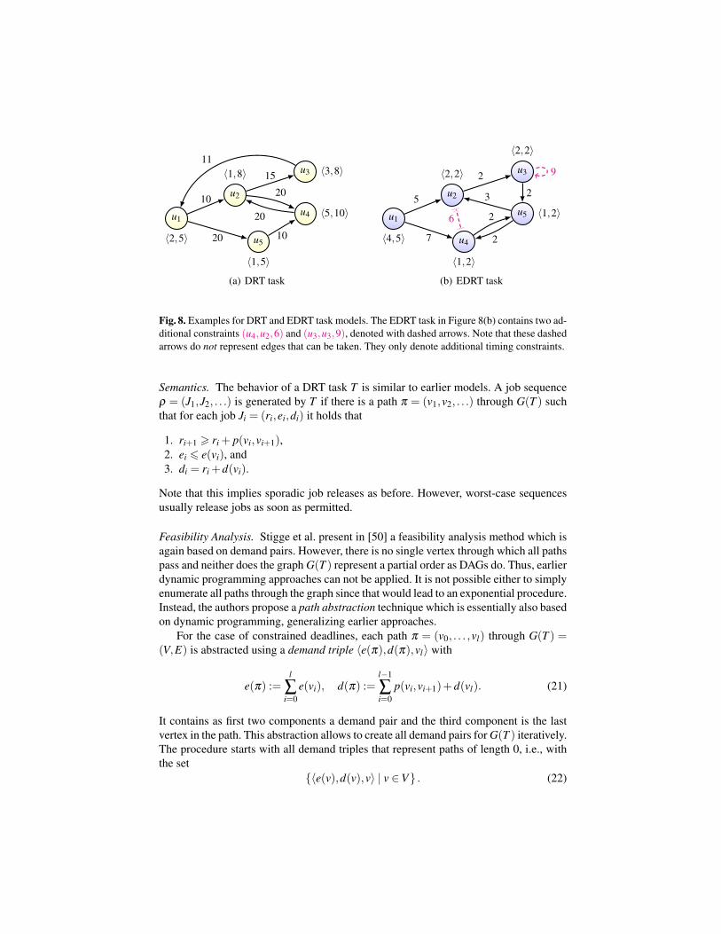
Fig. 8. Examples for DRT and EDRT task models. The EDRT task in Figure 8(b) contains two ad-ditional constraints (u4,u2,6) and (u3,u3,9), denoted with dashed arrows. Note that these dashedarrows do not represent edges that can be taken. They only denote additional timing constraints.

Semantics. The behavior of a DRT task T is similar to earlier models. A job sequenceρ = (J1,J2, . . .) is generated by T if there is a path π = (v1,v2, . . .) through G(T ) suchthat for each job Ji = (ri,ei,di) it holds that

1. ri+1 > ri + p(vi,vi+1),2. ei 6 e(vi), and3. di = ri +d(vi).

Note that this implies sporadic job releases as before. However, worst-case sequencesusually release jobs as soon as permitted.

Feasibility Analysis. Stigge et al. present in [50] a feasibility analysis method which isagain based on demand pairs. However, there is no single vertex through which all pathspass and neither does the graph G(T ) represent a partial order as DAGs do. Thus, earlierdynamic programming approaches can not be applied. It is not possible either to simplyenumerate all paths through the graph since that would lead to an exponential procedure.Instead, the authors propose a path abstraction technique which is essentially also basedon dynamic programming, generalizing earlier approaches.

For the case of constrained deadlines, each path π = (v0, . . . ,vl) through G(T ) =(V,E) is abstracted using a demand triple 〈e(π),d(π),vl〉 with

e(π) :=l

∑i=0

e(vi), d(π) :=l−1

∑i=0

p(vi,vi+1)+d(vl). (21)

It contains as first two components a demand pair and the third component is the lastvertex in the path. This abstraction allows to create all demand pairs for G(T ) iteratively.The procedure starts with all demand triples that represent paths of length 0, i.e., withthe set

{〈e(v),d(v),v〉 | v ∈V} . (22)

In each step, a triple 〈e,d,v〉 is picked from the set and extended to create new triples〈e′,d′,v′〉 via

e′ := e+ e(v′), d′ := d−d(v)+ p(v,v′)+d(v′), (v,v′) ∈ E. (23)

This is done for all edges (v,v′) ∈ E. The procedure abstracts from concrete paths sincethe creation of each new triple 〈e′,d′,v′〉 does not need the information of the full pathrepresented by 〈e,d,v〉. Instead, the last vertex v of any such path suffices. The authorsshow that this procedure is efficient since it only needs to be executed once up to abound D as before and the number of demand triples is bounded.

Further contributions of [50] include an extension of the method to arbitrary dead-lines and a few optimisation suggestions for implementations. One of them is consid-ering critical demand triples 〈e,d,v〉 for which no other demand triple 〈e′,d′,v′〉 existswith

1. e′ > e,2. d′ 6 d, and3. v′ = v.

It is shown that only critical demand triples need to be stored during the procedure.All other, non-critical, demand triples can be discarded since they and all their futureextensions will be dominated by others when considering contributions to the demandbound function dbf T (t). This optimization reduces the cubic time complexity of thealgorithm to about quadradic in the task parameters.

The presented method is applicable to all models in the previous sections since DRTgeneralizes all of them. In a few special cases, custom optimizations may speed up theprocess.

Static Priorities. Even though sufficient tests involving rbf (t) and dbf (t) similar toConditions (19) and (20) can be applied to DRT as well, no exact schedulability test forDRT with static priorities is currently known. It was shown in [52] that the problem isstrongly NP-hard via a reduction from the 3-PARTITION problem. This implies that anexact test with pseudo-polynomial complexity is impossible, assuming P 6=NP. Further,even fully polynomial-time approximation schemes can not exist either. The result holdsfor all models at least as expressive as GMF.

4.6 Global Timing Constraints

In an effort to investigate the border of how far graph-based workload models can begeneralized before the feasibility problem becomes infeasible, Stigge et al. propose in[49] a task model called Extended DRT (EDRT). In addition to a graph G(T ) as in theDRT model, a task T also includes a set C(T ) = {(from1, to1,γ1), . . . ,(fromk, tok,γk)}of global inter-release separation constraints. Each constraint (fromi, toi,γi) expressesthat between the visits of vertices fromi and toi, at least γi time units must pass. Anexample is shown in Figure 8(b).

Feasibility Analysis. The feasibility analysis problem for EDRT indeed marks thetractability borderline. In case the number of constraints in C(T ) is bounded by a con-stant k which is a restriction called k-EDRT, [49] presents a pseudo-polynomial fea-sibility test. If the number is not bounded, they show that feasibility analysis becomesstrongly NP-hard by a reduction from the Hamiltonian Path problem, ruling out pseudo-polynomial methods.

For the bounded case, we illustrate why the iterative procedure described in Sec-tion 4.5 for DRT can not be applied directly and then sketch a solution approach. Thedemand triple method can not be applied without change since the abstraction loses toomuch information from concrete paths. In the presence of global constraints, the proce-dure needs to keep track of which constraints are active. Consider path π =(u4,u5) fromthe example in Figure 8(b), which would be abstracted with demand triple 〈2,4,u5〉.An extension with u2 leading to demand triple 〈4,7,u2〉 is not correct, since the pathπ ′ = (u4,u5,u2) includes a global constraint, separating releases of the jobs associatedwith u4 and u2 by 6 time units. A correct abstraction of π ′ would therefore be 〈4,8,u2〉,but it is impossible to construct that from 〈2,4,u5〉 which lost information about theactive constraint.

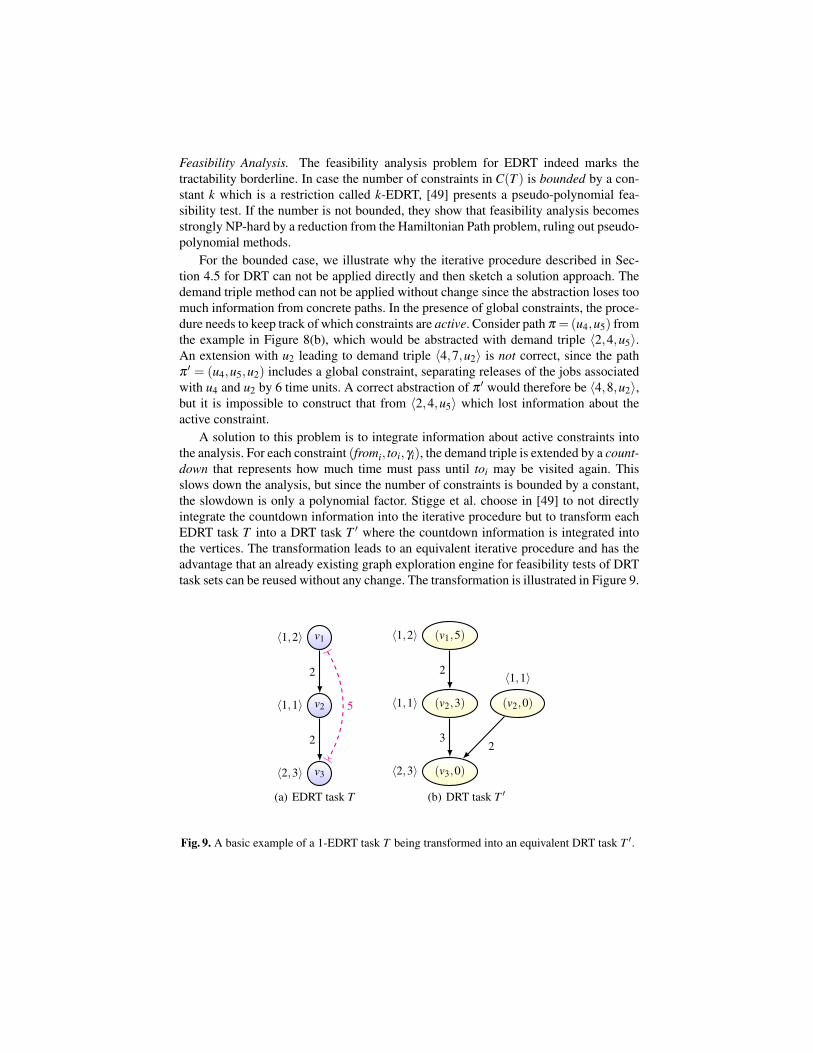
A solution to this problem is to integrate information about active constraints intothe analysis. For each constraint (fromi, toi,γi), the demand triple is extended by a count-down that represents how much time must pass until toi may be visited again. Thisslows down the analysis, but since the number of constraints is bounded by a constant,the slowdown is only a polynomial factor. Stigge et al. choose in [49] to not directlyintegrate the countdown information into the iterative procedure but to transform eachEDRT task T into a DRT task T ′ where the countdown information is integrated intothe vertices. The transformation leads to an equivalent iterative procedure and has theadvantage that an already existing graph exploration engine for feasibility tests of DRTtask sets can be reused without any change. The transformation is illustrated in Figure 9.

v1〈1,2〉

v2〈1,1〉

v3〈2,3〉

2

2

5

(a) EDRT task T

(v1,5)〈1,2〉

(v2,3)〈1,1〉

(v3,0)〈2,3〉

2

3

(v2,0)

〈1,1〉

2

(b) DRT task T ′

Fig. 9. A basic example of a 1-EDRT task T being transformed into an equivalent DRT task T ′.

5 Beyond DRT

We now turn to models that either extend the DRT model in other directions or areoutside the hierarchy in Figure 1 since they operate on a different abstraction level.

5.1 Task Automata

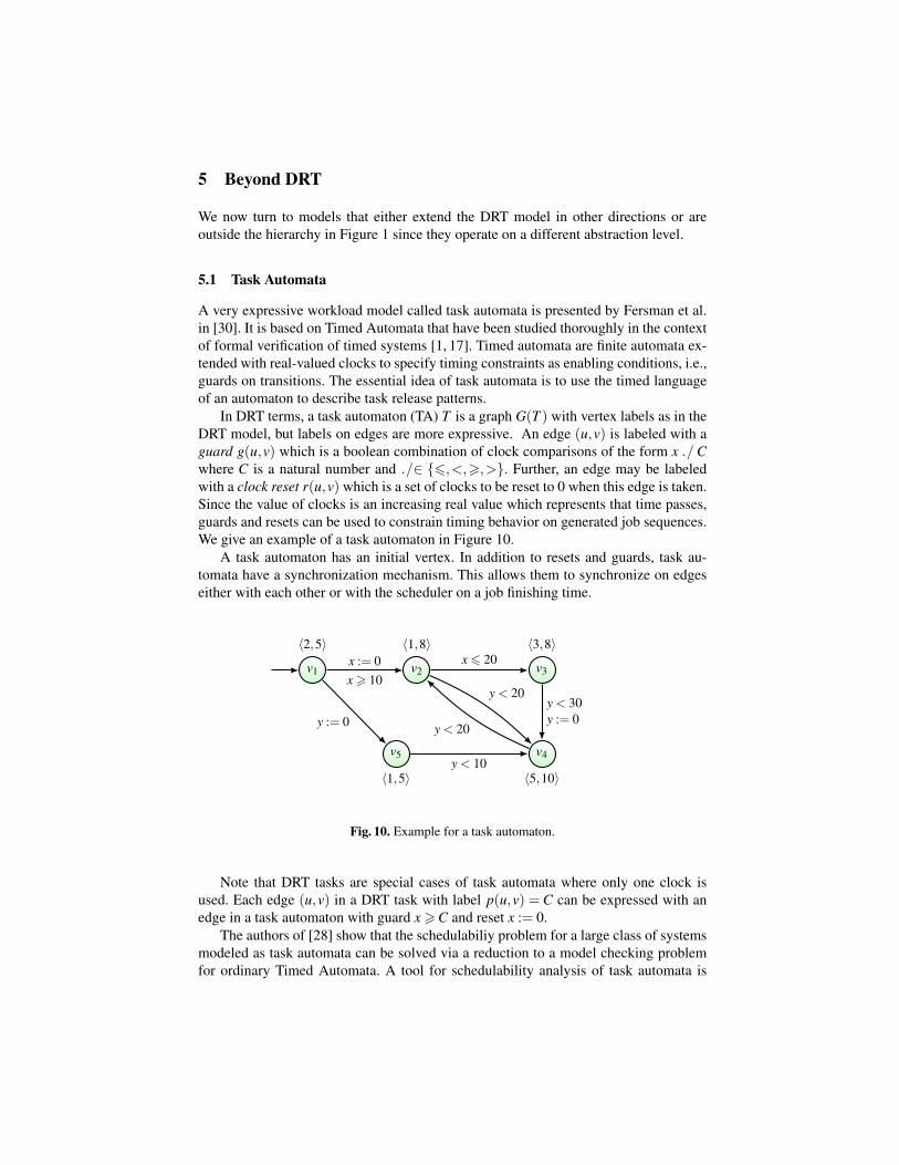
A very expressive workload model called task automata is presented by Fersman et al.in [30]. It is based on Timed Automata that have been studied thoroughly in the contextof formal verification of timed systems [1, 17]. Timed automata are finite automata ex-tended with real-valued clocks to specify timing constraints as enabling conditions, i.e.,guards on transitions. The essential idea of task automata is to use the timed languageof an automaton to describe task release patterns.

In DRT terms, a task automaton (TA) T is a graph G(T ) with vertex labels as in theDRT model, but labels on edges are more expressive. An edge (u,v) is labeled with aguard g(u,v) which is a boolean combination of clock comparisons of the form x ./Cwhere C is a natural number and ./∈ {6,<,>,>}. Further, an edge may be labeledwith a clock reset r(u,v) which is a set of clocks to be reset to 0 when this edge is taken.Since the value of clocks is an increasing real value which represents that time passes,guards and resets can be used to constrain timing behavior on generated job sequences.We give an example of a task automaton in Figure 10.

A task automaton has an initial vertex. In addition to resets and guards, task au-tomata have a synchronization mechanism. This allows them to synchronize on edgeseither with each other or with the scheduler on a job finishing time.

v1

〈2,5〉

v2

〈1,8〉

v3

〈3,8〉

v4

〈5,10〉

v5

〈1,5〉

x := 0x > 10

x 6 20

y < 20

y < 20y := 0y < 30y := 0

y < 10

Fig. 10. Example for a task automaton.

Note that DRT tasks are special cases of task automata where only one clock isused. Each edge (u,v) in a DRT task with label p(u,v) = C can be expressed with anedge in a task automaton with guard x >C and reset x := 0.

The authors of [28] show that the schedulabiliy problem for a large class of systemsmodeled as task automata can be solved via a reduction to a model checking problemfor ordinary Timed Automata. A tool for schedulability analysis of task automata is

presented in [2, 29]. In fact, the feasibility problem is decidable for systems where atmost two of the following conditions hold:

Preemption. The scheduling policy is preemptive.Variable Execution Time. Jobs may an interval of possible execution times.Task Feedback. The finishing time of a job may influence new job releases.

However, the feasibility problem is undecidable if all three conditions are true [28]. Taskautomata therefore mark a borderline between decidable and undecidable problems forworkload models.

5.2 Real-Time Calculus

A more abstract formalism to model real-time workload is the Real-Time Calculus(RTC) introduced in [55]. Its abstractions are based on the notions of

Event streams, representing the workload,Computing capacity, representing the computing resource for the workload, andProcessing units, modeling the process of the workload being executed, using up com-

puting capacity.

Formally, a request function R(t) models the accumulated amount of workload up toa time point t, and similarly, a capacity function C(t) models the amount of computa-tion resource available until time t. Both functions are the inputs to a processing unit,which outputs a new event stream modeled by a function R′(t), and leaves remainingcomputing capacity modeled by C′(t). The four functions are related by

R′(t) = min06u6t

{R(u)+C(t)−C(u)} , (24)

C′(t) =C(t)−R(t). (25)

Modeling static priority scheduling is rather straight forward in this model by creat-ing a number of processing units which all have their own input of request functions(representing different tasks) but all being chained through the corresponding capacityfunctions, i.e., C′(t) of one unit being C(t) of the next one. Other schedulers can alsobe modeled, with more involved constructions.

A concrete system may create many different request functions R(t). In order torepresent these, Real-Time Calculus considers upper and lower bounds in the time in-terval domain. Specifically, for abstracting the request function R(t), two arrival curvesαu(∆) and α l(∆) are introduced, so that for all t > 0 and ∆ > 0

αl(∆)6 R(t +∆)−R(t)6 α

u(∆). (26)

Clearly, a pair (αu,α l) abstracts an infinite set of event streams. Analogously, a pair ofservice curves (β u,β l) is defined in the time domain to abstract computing capacity.

All analysis can be executed on the level of arrival and service curves. For example,the remaining service curve can be computed via

βl′(∆) = max

06u6∆

{β

l(u)−αu(u)

}. (27)

Response-time analysis can be performed by deriving the response time from the hori-zontal distance between αu and β l .

For many classes of systems, arrival curves can be specified directly with closedform expressions. This includes the sporadic task model with an expression similar to(2), but is also possible for related models like periodic events with jitter [46].

It is worth noting that arrival curves and the request bound function introduced ear-lier are equivalent concepts. However, RTC models systems are directly using arrivalcurves, i.e., they are the low-level construct used for system representation. In contrast,the request bound function (and similarly, the demand bound function) is a tool forschedulability analysis that abstracts from a more concrete system description. It is apotentially overapproximate abstraction and the process of deriving request and demandbound functions for task models presented in Sections 3 and 4 is more or less computa-tionally demanding. Thus, the advantage of RTC is that arrival curves can be assumedas given input to the analysis procedures, at the cost of introducing imprecision.

6 Conclusions and Outlook

This survey is by no means complete. In preparing this paper, we have intended tocover only works on independent tasks for preemptive uniprocessors. Other sourcesfor a survey on related topics can be found in [5] on the broad area of static-priorityscheduling and analysis, [8] on scheduling and analysis of repetitive models for pre-emptable uniprocessors, [22] on real-time scheduling for multiprocessors and [48] onthe historic development of real-time systems research in general. To complement thesurvey provided by [8], we have added recent work on models with richer structures,that are based on graphs and automata as well as the Real-Time Calculus based on func-tions. Apart from their importance in theoretical studies, we believe that these expres-sive models may find their applications in for example model- and component-baseddesign for timed systems.

The following is a list of areas that we consider important, but did not include themin this paper due to time and page limits.

Resource Sharing. Real-time systems even on uniprocessor platforms contain not onlythe execution processor, but often many resources shared by concurrently running jobsusing a locking mechanism during their execution. Locking can introduce unwantedeffects like deadlocks and priority inversion. For periodic and sporadic task systems,the Priority Ceiling (and Inheritance) Protocols [47] and Stack Resource Policy [6]are established solutions with efficient schedulability tests. While these protocols canbe used for more expressive models like DRT, the analysis methods do not necessarilyapply. Some initial work exists on extending the classical results to graph-based models,e.g., [31] which develops a new protocol to deal with branching structures. The non-deterministic behaviours introduced by DRT-like models are not well understood in thecontext of resource sharing.

Real-Time Multiprocessor Scheduling. In contrast to uniprocessor systems, schedul-ing real-time workloads on parallel architectures is a much harder challenge. There are

various scheduling strategies, e.g., global and partition-based scheduling with mostlysufficient conditions for schedulability tests. A comprehensive survey on this topic isfound in [22]. The introduction of multicore platforms adds another dimension of com-plexity due to on-chip resource contention. The known techniques for multiprocessorscheduling all rely on a safe WCET bound of tasks under idealized assumptions on theunderlying platform. For multicore platforms, without proper isolation, it seems im-possible to achieve WCET bounds for tasks running in parallel on different processorcores. To the best of our knowledge, there is no work on bridging WCET analysis andmultiprocessor scheduling.

Mixed-Criticality Systems. Integrating applications of different levels of criticality onthe same processor chip is attracting increasing interest. Scheduling mixed-criticalityworkloads on uniprocessors has been studied intensively in recent years [15, 16, 26].For multiprocessor systems, it is still an open area for research; a seminal work is foundin [39]. Due to their potentially high computing capacity, we believe that multicoreprocessors are more adequate for such mixed types of applications. Typically, a mixedcriticality system operates in different modes. In the normal mode, the computationpower of multicores may be used to improve the average performance of low-criticalityapplications and in case of exceptions, e.g., a timing error occurs, high-criticality ap-plications should be prioritized. However, it is not well understood how to isolate andavoid interferences among the applications without fully partitioning the on-chip re-sources.

Further extensions of workload models. One may add new features or high-level struc-tures on the existing models for expressiveness and abstraction purposes. We see twointeresting directions:

Fork-Join Real-Time (FJRT) tasks: Recently, an extension of the DRT task model toincorporate fork/join structures is proposed by Stigge et al. Instead of following justone path through the graph, the behavior of a task includes the possibility of forkinginto different paths at certain nodes, and joining these paths later. Syntactically, thisis represented using hyperedges. A hypergraph generalizes the notion of a graphby extending the concept of an edge between two vertices to hyperedges betweentwo sets of vertices. For details, we refer to [51]. The model is illustrated withan example in Figure 11. For the time of writing this survey, no efficient analysismethod for FJRT is known.

Mode Switches: A system may operate in different modes demonstrating differenttiming behaviours. We consider a simple model using general directed graphs wherethe nodes stand for modes, assigned with a set of tasks to be executed in the corre-sponding mode, and edges for mode switches that may be triggered by an internalor external event and guarded by a timing constraint such as a minimal separationdistance. Mode switching is a concept that has been studied in different contexts.Many protocols for mode switches have been proposed [45] to specify what shouldbe done during the switch. In a recent work [27], the authors show that a mixedcriticality task system can be modeled nicely using a chain of modes representingthe criticality levels where mode switches are triggered by a task over-run that may

v1

v2 v3

v4

v5

v6

2

3

6

5 8

Fig. 11. Example FJRT task. The fork edge is depicted with an intersecting double line, the joinedge with an intersecting single line. All edges are annotated with minimum inter-release delaysp(U,V ). The vertex labels are omitted in this example. Assuming that vertex vi releases a jobof type Ji, a possible job sequence containing jobs with their types and absolute release times isσ = [(J1,0),(J2,5),(J5,5),(J4,6),(J3,7),(J5,8),(J6,16),(J1,22)].

occur at any time, and on each mode switch, tasks of lower-level criticality willbe dropped and only tasks of higher-level criticality are scheduled to run accord-ing to their new task parameters in the new mode. The authors present a techniquefor scheduling the mixed criticality workload described in directed acyclic graphs.An interesting direction for future work is scheduling of mode switches in generaldirected graphs, which involves fixed-point computation due to cyclic structures.

Tools for schedulability analysis. Over the years, many models and analysis techniqueshave been developed. It is desirable to have a software tool that as input takes a work-load description in some of the models and a scheduling policy and determines theschedulability. A tool for task automata has been developed using techniques for modelchecking timed automata [2]. Due to the analysis complexity of timed automata, it suf-fers from the state-explosion problem. For the tractable models including DRT in thehierarchy of Figure 1, a tool for schedulability analysis is currently under developmentin Uppsala based on the path abstraction technique of [50].

References

1. Rajeev Alur and David L. Dill. A Theory of Timed Automata. Theoretical Computer Science,126:183–235, 1994.

2. Tobias Amnell, Elena Fersman, Leonid Mokrushin, Paul Pettersson, and Wang Yi. TIMES -A Tool for Modelling and Implementation of Embedded Systems. In Proc. of TACAS 2002,pages 460–464. Springer-Verlag, 2002.

3. N.C. Audsley, A. Burns, M. F. Richardson, and A. J. Wellings. Hard Real-Time Scheduling:The Deadline-Monotonic Approach. In Proc. of RTOSS 1991, pages 133–137, 1991.

4. Neil Audsley. On priority assignment in xed priority scheduling. Information ProcessingLetters, 79(1):39–44, 2001.

5. Neil C Audsley, Alan Burns, Robert I Davis, Ken W Tindell, and Andy J Wellings. Fixedpriority pre-emptive scheduling: An historical perspective. Real-Time Systems, 8(2):173–198, 1995.

6. T. P. Baker. Stack-based scheduling for realtime processes. Real-Time Syst., 3(1):67–99,April 1991.

7. Sanjoy Baruah, Deji Chen, Sergey Gorinsky, and Aloysius Mok. Generalized multiframetasks. Real-Time Syst., 17(1):5–22, 1999.

8. Sanjoy Baruah and Joel Goossens. Scheduling real-time tasks: Algorithms and complexity.Handbook of Scheduling: Algorithms, Models, and Performance Analysis, 3, 2004.

9. Sanjoy K. Baruah, , A.K. Mok, and L.E. Rosier. Preemptively scheduling hard-real-timesporadic tasks on one processor. In Proc. of RTSS 1990, pages 182–190, 1990.

10. Sanjoy K. Baruah. A general model for recurring real-time tasks. In Proc. of RTSS, pages114–122, 1998.

11. Sanjoy K. Baruah. Feasibility Analysis of Recurring Branching Tasks. In Proc. of EWRTS,pages 138–145, 1998.

12. Sanjoy K. Baruah. Dynamic- and Static-priority Scheduling of Recurring Real-time Tasks.Real-Time Systems, 24(1):93–128, 2003.

13. Sanjoy K. Baruah. Preemptive Uniprocessor Scheduling of Non-cyclic GMF Task Systems.In Proc. of RTCSA 2010, pages 195–202, 2010.

14. Sanjoy K. Baruah. The Non-cyclic Recurring Real-Time Task Model. In Proc. of RTSS2010, pages 173–182, 2010.

15. Sanjoy K. Baruah, Vincenzo Bonifaci, Gianlorenzo D’Angelo, Haohan Li, AlbertoMarchetti-Spaccamela, Nicole Megow, and Leen Stougie. Scheduling real-time mixed-criticality jobs. IEEE Trans. Computers, 61(8):1140–1152, 2012.

16. Sanjoy K. Baruah, Alan Burns, and Robert I. Davis. Response-time analysis for mixedcriticality systems. In RTSS, pages 34–43, 2011.

17. Johan Bengtsson and Wang Yi. Timed automata: Semantics, algorithms and tools. In Lec-tures on Concurrency and Petri Nets, pages 87–124, 2003.

18. Vandy Berten and Joel Goossens. Sufficient FTP Schedulability Test for the Non-CyclicGeneralized Multiframe Task Model. CoRR, abs/1110.5793, 2011.

19. J.Y.L. Boudec and P. Thiran. Network Calculus: A Theory of Deterministic Queuing Systemsfor the Internet. Lecture Notes in Computer Science. Springer, 2001.

20. G.C. Buttazzo. Hard Real-Time Computing Systems: Predictable Scheduling Algorithms andApplications. Realtime Systems. Springer, 2011.

21. Samarjit Chakraborty, Thomas Erlebach, and Lothar Thiele. On the complexity of schedulingconditional real-time code. In Proc. of WADS 2001, pages 38–49, 2001.

22. Robert I. Davis and Alan Burns. A survey of hard real-time scheduling for multiprocessorsystems. ACM Comput. Surv., 43(4):35:1–35:44, October 2011.

23. T. Ebenlendr, M. Krcal, and J. Sgall. Graph balancing: A special case of scheduling unrelatedparallel machines. Algorithmica, pages 1–19, 2012. (Extended abstract published in theSODA 2008 Proceedings).

24. Friedrich Eisenbrand and Thomas Rothvoß. Static-priority Real-time Scheduling: ResponseTime Computation is NP-hard. In Proc. of RTSS 2008, pages 397–406, 2008.

25. Friedrich Eisenbrand and Thomas Rothvoß. EDF-schedulability of synchronous periodictask systems is coNP-hard. In Proc. of SODA 2010, pages 1029–1034, 2010.

26. Pontus Ekberg and Wang Yi. Outstanding paper award: Bounding and shaping the demandof mixed-criticality sporadic tasks. In ECRTS, pages 135–144, 2012.

27. Pontus Ekberg and Wang Yi. Bounding and shaping the demand of generalized mixed-criticality sporadic task systems. Norwell, MA, USA, 2013. Kluwer Academic Publishers.

28. Elena Fersman, Pavel Krcal, Paul Pettersson, and Wang Yi. Task automata: Schedulability,decidability and undecidability. Inf. Comput., 205(8):1149–1172, 2007.

29. Elena Fersman, Leonid Mokrushin, Paul Pettersson, and Wang Yi. Schedulability analysisof fixed-priority systems using timed automata. Theor. Comput. Sci., 354(2):301–317, 2006.

30. Elena Fersman, Paul Pettersson, and Wang Yi. Timed Automata with Asynchronous Pro-cesses: Schedulability and Decidability. In Proc. of TACAS 2002, pages 67–82. Springer-Verlag, 2002.

31. Nan Guan, Pontus Ekberg, Martin Stigge, and Wang Yi. Resource Sharing Protocols forReal-Time Task Graph Systems. In Proc. of ECRTS 2011, pages 272–281, 2011.

32. C.-C. J. Han. A Better Polynomial-Time Schedulability Test for Real-Time MultiframeTasks. In Proc. of RTSS, pages 104–, Washington, DC, USA, 1998. IEEE Computer So-ciety.

33. Mathai Joseph and Paritosh K. Pandya. Finding Response Times in a Real-Time System.The Computer Journal, 29:390–395, 1986.

34. Edward A. Lee, Stephen Neuendorffer, and Michael J. Wirthlin. Actor-oriented design ofembedded hardware and software systems. Journal of Circuits, Systems, and Computers, 2,2003.

35. John P. Lehoczky, Lui Sha, and Jay K. Strosnider. Enhanced Aperiodic Responsiveness inHard Real-Time Environments. In Proc. of RTSS, pages 261–270, 1987.

36. J.K. Lenstra, A.H.G. Rinnooy Kan, and P. Brucker. Complexity of machine schedulingproblems. Annals of Discrete Mathematics, 1:343–362, 1977.

37. Joseph Y.-T. Leung and M.L. Merrill. A note on preemptive scheduling of periodic, real-timetasks. Information Processing Letters, 11(3):115 – 118, 1980.

38. Joseph Y.-T. Leung and Jennifer Whitehead. On the complexity of fixed-priority schedulingof periodic, real-time tasks. Performance Evaluation, 2(4):237 – 250, 1982.

39. Haohan Li and Sanjoy K. Baruah. Outstanding paper award: Global mixed-criticalityscheduling on multiprocessors. In ECRTS, pages 166–175, 2012.

40. C. L. Liu and James W. Layland. Scheduling Algorithms for Multiprogramming in a Hard-Real-Time Environment. J. ACM, 20(1):46–61, 1973.

41. Wan-Chen Lu, Kwei-Jay Lin, Hsin-Wen Wei, and Wei-Kuan Shih. New Schedulability Con-ditions for Real-Time Multiframe Tasks. In Proc. of ECRTS, pages 39–50, 2007.

42. A. K. Mok. Fundamental Design Problems of Distributed Systems for The Hard-Real-TimeEnvironment. Technical report, Cambridge, MA, USA, 1983. Ph.D. thesis.

43. Aloysius K. Mok and Deji Chen. A General Model for Real-Time Tasks. Technical report,1996.

44. Aloysius K. Mok and Deji Chen. A Multiframe Model for Real-Time Tasks. IEEE Trans.Softw. Eng., 23(10):635–645, 1997.

45. L.T.X. Phan, Insup Lee, and O. Sokolsky. A semantic framework for mode change protocols.In Real-Time and Embedded Technology and Applications Symposium (RTAS), 2011 17thIEEE, pages 91 –100, april 2011.

46. Kai Richter. Compositional Scheduling Analysis Using Standard Event Models. PhD thesis,Technical University of Braunschweig, Braunschweig, Germany, 2004.

47. L. Sha, R. Rajkumar, and J.P. Lehoczky. Priority inheritance protocols: an approach to real-time synchronization. Computers, IEEE Transactions on, 39(9):1175 –1185, sep 1990.

48. Lui Sha, Tarek Abdelzaher, Karl-Erik Arzen, Anton Cervin, Theodore Baker, Alan Burns,Giorgio Buttazzo, Marco Caccamo, John Lehoczky, and Aloysius K. Mok. Real timescheduling theory: A historical perspective. Real-Time Syst., 28(2-3):101–155, November2004.

49. Martin Stigge, Pontus Ekberg, Nan Guan, and Wang Yi. On the Tractability of Digraph-Based Task Models. In Proc. of ECRTS 2011, pages 162–171, 2011.

50. Martin Stigge, Pontus Ekberg, Nan Guan, and Wang Yi. The Digraph Real-Time Task Model.In Proc. of RTAS 2011, pages 71–80, 2011.

51. Martin Stigge, Pontus Ekberg, and Wang Yi. The Fork-Join Real-Time Task Model. In Proc.of ACM SIGBED Review, 2012. To appear.

52. Martin Stigge and Wang Yi. Hardness Results for Static Priority Real-Time Scheduling. InProc. of ECRTS 2012, pages 189–198, 2012.

53. Hiroaki Takada and Ken Sakamura. Schedulability of Generalized Multiframe Task Setsunder Static Priority Assignment. In Proc. of RTCSA 1997, pages 80–86, 1997.

54. Noel Tchidjo Moyo, Eric Nicollet, Frederic Lafaye, and Christophe Moy. On SchedulabilityAnalysis of Non-cyclic Generalized Multiframe Tasks. In ECRTS 2010, pages 271–278,2010.

55. L. Thiele, S. Chakraborty, and M. Naedele. Real-time calculus for scheduling hard real-timesystems. In ISCAS 2000, volume 4, 2000.

56. Jose Verschae and Andreas Wiese. On the configuration-lp for scheduling on unrelatedmachines. In ESA, pages 530–542, 2011.

57. Tei wei Kuo, Li pin Chang, Yu hua Liu, and Kwei jay Lin. Efficient online schedulabilitytests for real-time systems. IEEE Transactions On Software Engineering, 29:734–751, 2003.

58. A. Zuhily and A. Burns. Exact Scheduling Analysis of Non-Accumulatively MonotonicMultiframe Tasks. Real-Time Systems Journal, 43:119–146, 2009.