models and solution approaches for development …
TRANSCRIPT
MODELS AND SOLUTION APPROACHES FOR DEVELOPMENT AND
INSTALLATION OF PEV INFRASTRUCTURE
A Dissertation
by
SEOK KIM
Submitted to the Office of Graduate Studies of
Texas A&M University
in partial fulfillment of the requirements for the degree of
DOCTOR OF PHILOSOPHY
December 2011
Major Subject: Civil Engineering

Models and Solution Approaches for Development and Installation of PEV
Infrastructure
Copyright by Seok Kim 2011
MODELS AND SOLUTION APPROACHES FOR DEVELOPMENT AND
INSTALLATION OF PEV INFRASTRUCTURE
A Dissertation
by
SEOK KIM
Submitted to the Office of Graduate Studies of
Texas A&M University
in partial fulfillment of the requirements for the degree of
DOCTOR OF PHILOSOPHY
Approved by:
Chair of Committee, Ivan Damnjanovic
Committee Members, Stuart D. Anderson
Luca Quadrifoglio
Mladen Kezunovic
Head of Department, John Niedzwecki
December 2011
Major Subject: Civil Engineering
iii
ABSTRACT
Models and Solution Approaches for Development and Installation of PEV
Infrastructure. (December 2011)
Seok Kim,
B.S., Chung-Ang University; M.S., Chung-Ang University
Chair of Advisory Committee: Dr. Ivan Damnjanovic
This dissertation formulates and develops models and solution approaches for
plug-in electric vehicle (PEV) charging station installation. The models are formulated
in the form of bilevel programming and stochastic programming problems, while a meta-
heuristic method, genetic algorithm, and Monte Carlo bounding techniques are used to
solve the problems.
Demand for PEVs is increasing with the growing concerns about environmental
pollution, energy resources, and the economy. However, battery capacity in PEVs is still
limited and represents one of the key barriers to a more widespread adoption of PEVs. It
is expected that drivers who have long-distance commutes hesitate to replace their
internal combustion engine vehicles with PEVs due to range anxiety. To address this
concern, PEV infrastructure can be developed to provide re-fully status when they are
needed.
This dissertation is primarily focused on the development of mathematical
models that can be used to support decisions regarding a charging station location and
iv
installation problem. The major parts of developing the models include identification of
the problem, development of mathematical models in the form of bilevel and stochastic
programming problems, and development of a solution approach using a meta-heuristic
method.
PEV parking building problem is formulated as a bilevel programming problem
in order to consider interaction between transportation flow and a manager decisions,
while the charging station installation problem is formulated as a stochastic
programming problem in order to consider uncertainty in parameters. In order to find the
best-quality solution, a genetic algorithm method is used because the formulation
problems are NP-hard. In addition, the Monte Carlo bounding method is used to solve
the stochastic program with continuous distributions.
Managerial implications and recommendations for PEV parking building
developers and managers are suggested in terms of sensitivity analysis. First, in the
planning stage, the developer of the PEV parking building should consider long-term
changes in future traffic flow and locate a PEV parking building closer to the node with
the highest destination trip rate. Second, to attract more parking users, the operator needs
to consider the walkability of walking links.

v
DEDICATION
To my wife and family

vi
ACKNOWLEDGEMENTS
First and foremost, I would like to thank Dr. Ivan Damnjanovic, chairman of my
academic committee and the driving force behind this research effort. Dr. Damnjanovic
contributed valuable ideas while being very receptive to my suggestions, and provided
his typical unwavering support and exemplary leadership that was indispensable to the
successful completion of this research. To other members of my academic committee:
Dr. Stuart D. Anderson, Luca Quadrifoglio, and Mladen Kezunovic, I would like to say a
big thank you for your support throughout my Ph.D. study.
I also acknowledge the support and inspiration of my family, especially my wife,
Jinhee Kim, for her understanding and love during the past few years. Her support and
encouragement were in the end what made this dissertation possible. My parents, Tae-
Wook and Ok-Sun, receive my deepest gratitude and love for their dedication and their
many years of support during my studies.
vii
TABLE OF CONTENTS
Page
ABSTRACT .............................................................................................................. iii
DEDICATION .......................................................................................................... v
ACKNOWLEDGEMENTS ...................................................................................... vi
TABLE OF CONTENTS .......................................................................................... vii
LIST OF FIGURES ................................................................................................... x
LIST OF TABLES .................................................................................................... xiii
1. INTRODUCTION ............................................................................................... 1
1.1 Background and Research Motivation ................................................. 1
1.2 Research Objectives ............................................................................. 4
1.3 Scope of the Study ................................................................................ 5
1.4 Overview of Study Approach ............................................................... 6
1.4.1 PEV Infrastructure Development Problem ................................. 7
1.4.2 Model for Impact of PEV Infrastructure ..................................... 8
1.4.3 PEV Charging Station Installation Problem ................................ 8
1.4.4 Solution Approaches ................................................................... 9
1.5 Dissertation Outline .............................................................................. 9
2. LITERATURE REVIEW .................................................................................... 11
2.1 Facility Location Problem .................................................................... 11
2.2 Traffic Assignment ............................................................................... 13
2.3 Parking Choice Model .......................................................................... 15
2.4 Network Design Problem .................................................................... 17
2.5 Stochastic Programming ...................................................................... 18
2.6 Electricity Power Market ..................................................................... 19
2.7 Economic Dispatch and Locational Marginal Price ............................. 21
2.8 Summary .............................................................................................. 24
3. PEV PARKING BUILDING DEVELOPMENT PROBLEM ............................ 25
3.1 Problem Description ............................................................................. 25
viii
Page
3.2 The Model ............................................................................................ 29
3.2.1 Lower-Level Problem ................................................................. 32
3.2.2 Upper-Level Problem .................................................................. 36
3.3 Computational Study ............................................................................ 38
3.3.1 Simple Network ........................................................................... 39
3.3.2 Large Network ............................................................................. 47
3.4 Summary .............................................................................................. 51
4. IMPACT OF PEV ON ELECTRICITY NETWORK ......................................... 53
4.1 Problem Description ............................................................................. 53
4.2 The Model ............................................................................................ 55
4.2.1 Network Design Problem ............................................................ 56
4.2.2 Power System Operating Conditions .......................................... 57
4.3 Computational Study ............................................................................ 59
4.3.1 Simple Network ........................................................................... 59
4.3.2 Large Network ............................................................................. 71
4.4 Summary .............................................................................................. 85
5. CHARGING STATION INSTALLATION PROBLEM (TWO-STAGE
STOCHASTIC PROBLEM WITH SIMPLE RECOURSE) .............................. 86
5.1 Problem Description ............................................................................. 86
5.2 The Model ............................................................................................ 88
5.3 Monte Carlo Bounding Approach ........................................................ 91
5.4 Case Study ............................................................................................ 92
5.4.1Area Scope ................................................................................... 92
5.4.2Data .............................................................................................. 94
5.4.3Results .......................................................................................... 98
5.4.4 Sensitivity Analysis ..................................................................... 99
5.5 Summary .............................................................................................. 101
6. CHARGING STATION INSTALLATION PROBLEM WITH DECISION-
DEPENDENT ASSESSMENT OF UNCERTAINTY (TWO-STAGE
STOCHASTIC PROBLEM WITH RECOURSE) .............................................. 103
6.1 Problem Description ............................................................................. 103
6.2 The Model ............................................................................................ 106
6.3 Decision-Dependent Assessment of Uncertainty ................................. 107
6.4 Case Study ............................................................................................ 109
6.5 Summary .............................................................................................. 113
ix
Page
7. SUMMARY AND CONCLUSIONS .................................................................. 114
7.1 Overall Summary and Discussion ........................................................ 114
7.2 Recommendations for Future Research ............................................... 117
REFERENCES .......................................................................................................... 120
APPENDIX I ............................................................................................................. 130
APPENDIX II ........................................................................................................... 131
APPENDIX III .......................................................................................................... 132
APPENDIX IV .......................................................................................................... 133
APPENDIX V ........................................................................................................... 134
APPENDIX VI .......................................................................................................... 135
VITA ......................................................................................................................... 138

x
LIST OF FIGURES
FIGURE Page
1.1 Overall Study Approach ............................................................................. 7
2.1 Power Market Structure ............................................................................. 21
3.1 Roles of PEV Parking Building ................................................................. 26
3.2 Simple Transportation Network with PEV Parking Building .................... 27
3.3 Example of Demand of PEV Parking Building for One Day..................... 28
3.4 Simple Network .......................................................................................... 39
3.5 Demands of PEV Parking Building Depending on Location and
Incentive ..................................................................................................... 43
3.6 Fitness and Contour Graph for Total Revenue ........................................... 45
3.7 Results of Sensitivity Analysis ................................................................... 46
3.8 Sioux Falls Network ................................................................................... 48
3.9 Fitness Graph for Total Revenue ............................................................... 49
3.10 Results of Sensitivity Analysis ................................................................... 50
4.1 Schematic Representation of the Networks with PEV Parking Building .. 54
4.2 Example Networks ..................................................................................... 60
4.3 Power Load in V2G .................................................................................... 63
4.4 Power Generation in V2G .......................................................................... 64
4.5 LMP in V2G ............................................................................................... 66
4.6 Power Load in G2V .................................................................................... 67

xi
FIGURE Page
4.7 Power Generation in G2V .......................................................................... 68
4.8 LMP in G2V ............................................................................................... 69
4.9 Surface and Contour Graphs for Total Revenues ....................................... 70
4.10 IEEE 14 Bus Test System on Transportation Network in Sioux Falls ....... 72
4.11 Operating Areas for Each Bus .................................................................... 73
4.12 Limits of Operating Areas in Transportation Network .............................. 74
4.13 Fitness Graph for Total Revenue ............................................................... 77
4.14 Power Load in V2G of Large Network ...................................................... 79
4.15 Power Generation in V2G of Large Network ............................................ 80
4.16 LMP in V2G of Large Network ................................................................. 81
4.17 Power Load in G2V of Large Network ...................................................... 82
4.18 Power Generation in G2V of Large Network ............................................ 83
4.19 LMP in G2V of Large Network ................................................................. 84
5.1 Influence of Installation of Charging Stations ........................................... 87
5.2 Model Framework ...................................................................................... 88
5.3 Existing Parking Garages and Surface Parking Lots ................................. 93
5.4 Installation Cost .......................................................................................... 95
5.5 Utility Cost ................................................................................................. 96
5.6 Attraction Rate by Walking Distance ......................................................... 97
5.7 Distributions for Uncertain Parameter ....................................................... 98
5.8 Results of Sensitivity Analysis ................................................................... 100

xii
FIGURE Page
6.1 Model Framework ...................................................................................... 105
6.2 Procedure of Bayesian Updating ................................................................ 110
6.3 Fitness Graph for Total Cost ...................................................................... 111
xiii
LIST OF TABLES
TABLE Page
3.1 Link Data for Example Network ................................................................ 40
3.2 Forecasts of Power Price Used for Numerical Example ............................ 41
3.3 Methods and Parameters of GA Operators ................................................ 44
4.1 Generation Data for Example Network ...................................................... 61
4.2 Modified Generator Data ........................................................................... 75
4.3 Modified Branch Data ................................................................................ 75
4.4 Modified Generator Cost Data ................................................................... 76
5.1 Equations for Monte Carlo Bounding Method ........................................... 91
5.2 Parking Spaces ........................................................................................... 92
5.3 Walking Distances from Northgate Garage ............................................... 94
5.4 Result .......................................................................................................... 99
6.1 Methods and Parameters of GA Operators ................................................ 111
6.2 Result .......................................................................................................... 112
1
1. INTRODUCTION
1.1 Background and Research Motivation
Plug-in electric vehicles (PEVs), either as battery electric vehicles (BEVs) or
plug-in hybrid electric vehicles (PHEVs), have gained much attention as an effective
solution to growing concerns about energy security and environmental pollution.
Currently, the transportation sector accounts for more than half of the total liquid fuel
demand (U.S. Energy Information Administration 2009) and produces the highest
amount of CO2 emissions in the US—around 33% (Lilienthal and Brown 2007). PEVs
represent solution to these concerns in that they provide higher fuel efficiency and lower
greenhouse gas (GHG) emissions than internal combustion engine vehicles1 (ICEVs).
The market for PEVs has been steadily growing. Recently, rising gas prices have
made drivers consider a PEV as their next vehicle. Furthermore, federal and local
governments are now providing incentives for consumers to increase PEV sales,
including carpool lane access, rebates, and tax credits. Growing PEV demand also
encourages major automobile manufacturers to develop PEV models. Several
researchers have recently stated that the market share of PEVs will significantly increase
in the future. For example, Short and Denholm (2006) estimated that by 2030, the
market share of PEVs could reach 25%, and a technical report from the University of
Michigan (Sullivan et al. 2009) predicts that the market share of PHEVs could reach
around 20% by 2040, in an optimistic scenario.
1
This thesis follows the style of the Journal of Construction Engineering and Management.
2
The unique feature of PEVs—a connection to an electric power grid using a
plug—could bring significant benefits to electric power systems. Generally, when
electric power stored in PEVs flows to a power grid, it is called “vehicle-to-grid” (V2G).
The opposite flow of electric power is referred to as “grid-to-vehicle” (G2V). The
generating potential of V2G technology could be substantial. For instance, 150 PHEVs,
such as PHEV-40 or PHEV-60, which stand for a plug-in hybrid electric vehicle with 40
miles or 60 miles of electric only range, could provide 1 MW of power for several hours,
which is enough to support a large building (Solomon and Vincent 2003). Also, if all
light vehicle fleets in the United States connected to a power grid, the generated power
would be around seven times larger than the average national load (Kempton and Dhanju
2006). PEVs connected to a power grid could perform the role of a distributed generator,
which in turn could provide several advantages: improving efficiency of power
generation, making power grids more stable, and reducing the losses from transmission
and distribution systems (Stovall et al. 2005).
Further, PEVs play an important synergetic role in wind generation, thereby
helping with the difficulty in managing such sources of energy. Wind energy has been
regarded as one of the most powerful and renewable sources of energy. However, wind
energy has a reliability problem in that the production of electricity does not remain
consistent. As a solution for managing the supply of wind energy, Kempton and Tomic
(2005b) suggested that the V2G technology of PEVs can provide operating reserves and
storage to control the volatility of wind energy as well as that of other renewable energy
sources.

3
PEV infrastructure with the V2G mode has potential to develop a new business
model for vehicle charging. For example, Kempton and Tomic (2005a; 2005b) suggested
a PEV parking garage that could provide ancillary services of regulation, spinning
reserve, and peak power in the V2G mode as a business model. Similarly, Guille and
Gross (2009) proposed a framework to integrate the aggregated battery vehicles into the
electric power grid and presented the aggregated PEVs in a parking facility as one of the
electric power sources.
PEV infrastructure with the G2V mode would accelerate the increased PEV
adoption rate. Battery capacity in PEVs is one of the key barriers in the more widespread
adoption of PEV. Drivers who have long-distance commutes hesitate to replace their
ICEVs with PEVs due to range anxiety. In this situation, PEV infrastructure could
encourage people to replace their ICEVs with PEVs.
This research was motivated by the lack of advances in development of PEV
infrastructures. A PEV infrastructure represents an interface between a transportation
network and an electric power system. Developers of PEV infrastructures need to
carefully consider two different networks and systems at the construction planning stage.
However, little attention has been paid to the development of new PEV infrastructures
by concurrently considering behavior of two different networks and systems (i.e.
transportation and electric power flow).
Making sound decisions based on accurate estimates of cost and future revenue,
which occurs in the planning stage, is important for developing a new infrastructure that
is effective and beneficial to project developers. This study provides a basis for: a)
4
developing new parking infrastructures, and b) investigating the impact of those new
parking infrastructures on transportation and electric power system. The analyses are
limited to planning stage of project development.
The methodology developed through this research involves the integration of two
different networks and systems and a solution framework based on a genetic algorithm
and the Monte Carlo bounding technique.
1.2 Research Objectives
The main goal of this research is to develop strategic decision-support models for
PEV infrastructure development from a business proposition perspective, and to
investigate the impact of PEV infrastructures on the electric power market and
transportation system performance. The strategic decision models were created for
project developers or facility managers. More specifically, the research objectives and
issues are as follows:
Objective 1: Formulate a deterministic PEV infrastructure development
problem that can be used to make optimal decisions based on current traffic
and power system conditions. The PEV infrastructure location problem should
be able to take into account sensitivity of transportation network structure,
origin-destination trip rates, parking fee, and electric power price on
profitability of the project.
5
Objective 2: Formulate a stochastic PEV charging station installation problem
that can be used to determine the optimal number of charging stations to be
installed in existing parking buildings. The problem considers uncertainty on
PEV adoption rates, cost of installation, and opportunity cost of converting
existing parking spots that currently guarantee certain revenue.
Objective 3: Design meta-heuristic algorithms that can exploit problem
structure in solving the proposed problems (both small scale and large scale
networks) within a reasonable run time.
Objective 4: Develop a problem to investigate the impact of PEV
infrastructures on transportation networks and electric power systems. This is
an inverse problem of the problem in objective 1 where the focus is on private
development. The model should be able to provide optimal decisions
depending on different conditions, such as V2G with fixed power price, V2G
with locational marginal prices, and G2V with locational marginal prices.
1.3 Scope of the Study
The scope of the study is as follows:
The present study focuses on identifying optimal decisions for developing a
PEV infrastructure project and the impact of a PEV parking building on the
electric power market and transportation system.
6
The proposed problems were developed from the perspective of PEV
infrastructure developers and managers. Note that developers and managers can
make optimal decisions in order to increase their profit and decrease their cost.
The proposed problems are considered in project planning stage. The decisions
such as facility location, incentive structure, and the number of charging
stations, are usually made during the planning stage.
A PEV infrastructure serves as a parking facility and an electric aggregator1.
PEV developers and managers can make a profit from providing parking
service and charging service, as well as contracting with an independent system
operator (ISO) to sell electric power generated from vehicle batteries.
1.4 Overview of Study Approach
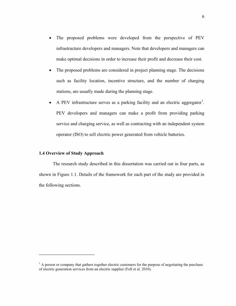
The research study described in this dissertation was carried out in four parts, as
shown in Figure 1.1. Details of the framework for each part of the study are provided in
the following sections.
1 A person or company that gathers together electric customers for the purpose of negotiating the purchase
of electric generation services from an electric supplier (Fell et al. 2010).
7
Figure 1.1 Overall Study Approach
1.4.1 PEV Infrastructure Development Problem
The PEV infrastructure development problem was formulated in the form of a
bilevel programming problem (BLPP). The traffic assignment problem is defined as a
lower-level problem and the business model as an upper-level problem. The traffic
assignment problem requires data and parameters, such as traffic counts, parking hours,
and network properties. The results of the traffic assignment problem, link flows
between nodes, were used to calculate the demand for a PEV parking building. The
business model consists of services provided by a PEV parking building: parking,
charging, regulation, and peak demand service. In addition, the business model requires
electric power price data and plausible PEV adoption rates.
TRAFFIC ASSIGNMENT
PROBLEM
Calculate
the demand of SG
BUSINESS MODEL
Traffic Counts
Incentive Structure of SGB
Location of SGB
DATA AND PEV SCENARIOS
Charging/Discharging Pattern
Penetration rate of PEV
Parking Fee
Peak Demand Service
(V2G)
Charging Service
(G2V)
Regulation Service
(G2V & V2G)
Locational Marginal Prices
Properties of Network
• Length of Links
• Capacity of Links
• Parameter α and β in link cost functions
Parking Fare
Link Flows between
Nodes
OPTIMAL DECISION
Average Speed of Vehicles and Pedestrians
Parking Hours
DATA AND PARAMETERS
MODEL FOR LMP
Based on Optimal Power Flow Problem
Generation from PEV Infrastructure
Load for Charging PEVs
Load Changed by Traffic Flow
Electric Power Network
Transmission Systems
Generation Data
Load on bus
DATA AND PARAMETERS
PEV INFRASTRUCTURE
DEVELOPMENT PROBLEM
The number of Charging
Stations
OPTIMAL DECISION
PEV CHARGING STATION
INSTALLATION PROBLEM
Calculate
the PEV parking demand
COST MODEL
Installation Cost
Utility Cost
SOLUTION METHOD
Meta-heuristic Method
8
1.4.2 Model for Impact of PEV Infrastructure
A PEV parking building can be considered as a power generation source, or
power load in an electric power network. Hence, PEV parking demand can change the
electric load on buses. The model developed in this study employs data such as trip rates
and power system operating conditions to calculate PEV parking demand and locational
marginal prices on buses, which can explain the impact of a PEV infrastructure on
transportation network and electric power network. The locational marginal prices are
used in the business model.
1.4.3 PEV Charging Station Installation Problem
The PEV charging station installation problem was formulated in the form of a
stochastic programming problem (SPP). In this study, two types of SPPs were designed:
a two-stage simple recourse, and a two-stage recourse problem. Two-stage simple
recourse model focuses on the first stage decisions and the consequence in the others. On
the other hand, two-stage recourse problem considers that the initial decision will affect
the decision in the second stage. To calculate PEV parking demand, data such as parking
demand, PEV penetration rate, and rate of willingness to charge are required. The total
cost is the sum of installation cost and utility cost calculated from the PEV parking
demand. The PEV charging station installation problem determines the number of
charging stations that constitute the optimal decision variables.

9
1.4.4 Solution Approaches
As it is very difficult to solve bilevel programming problems and stochastic
programs with continuous distributions, a meta-heuristic method was used in this study
to find the high-quality, optimal solution. Among meta-heuristic methods, the genetic
algorithm is a general method for searching the feasible landscape for highly fit
solutions. The genetic algorithm consists of three types of operators, including selection,
cross-over, and mutation.
Finally, a sensitivity analysis revealed some managerial implications for the
proposed problems in this study. Generally, sensitivity analysis provides a measure of
how the optimal decisions vary with the changes in the parameters and scenarios.
1.5 Dissertation Outline
This dissertation is organized in seven sections.
Section 1 reveals the background and research motivation, including the study
objectives, scope, and approach, and provides an outline of the research.
Section 2 reviews the conventional facility location problem, network design
problem, stochastic programming problem, and other related research efforts in
the electricity power market.
Section 3 describes the proposed model for developing a new PEV parking
building. In the model, interaction between a transportation network and an
electric power system is formulated in terms of a bilevel programming problem.
10
For a developer, managerial implications are suggested based on a sensitivity
analysis.
Section 4 focuses on an investigation of the impact of a PEV parking building
on an electric power system. To look into the impact, this study considered
locational marginal prices by integrating the PEV parking building problem in
Section 3 and a power flow analysis.
Section 5 presents a model for installing charging stations in an existing
parking building. The model was formulated in the form of the stochastic
programming problem in order to consider uncertainty in parameters.
Section 6 describes an improvement of the model in Section 5, in order to
explain the influence of the initial decision on uncertainty in parameters. The
framework of Bayesian updating of random parameters is described. The
model gives the best combination of two decisions: the number of initial
charging stations in the first stage and that of additional charging stations in the
second stage.
Section 7 discusses the achievement of research goals, contributions, and
limitations of developed problems. In addition, future research endeavors are
recommended.

11
2. LITERATURE REVIEW
This section presents an overview of the background literature on conventional
facility location problems, traffic assignment problem, parking choice model, network
design problems, stochastic programming problems, and other related research efforts on
modeling the electricity power market and price. Section 2.1 introduces a general
background of facility location problems and reviews continuous single facility location
problems. In Section 2.2, traffic assignment problem is introduced in terms of driver’s
behavior assumptions and time-dependency. Section 2.3 shows some parking choice
models and important factors for the models. In Section 2.4, a brief review of network
design problems and some applications are presented. Section 2.5 introduces a basic
formulations of a stochastic programming problem and presents some application areas
of the modeling formulations. Section 2.6 presents the power market analysis and
structure. Some basic equations to calculate economic generation plan and regional
electric power prices are shown in Section 2.7.
2.1 Facility Location Problems
Facility location problems can be used to determine the optimal location of
industrial or governmental buildings. Location decision has been shown to have an
influence on service cost and quality and is generally applied to hospital, warehouse, and
plant location problems. Location problems are classified as discrete and continuous
12
facility location problems. This section presents a brief background of continuous
facility location problems.
Since Alfred Weber (1909) first introduced the concept of finding optimal
location, location problems have been extensively used for determining facility location,
fire-station coverage, and in-network design problems. The objective of the Weber
problem, also known as the 1-median problem, is to find the location of a facility by
minimizing the sum of the weighted distances and is formulated as follows:
1
minn
i i
i
f x w x x
(2.1)
where, x is the location of the new facility; ix is the location of the existing facility;
ix x is the function of the distance between x and ix ; iw is the parameter used to
convert the distance to cost; and n is the number of existing facilities.
In a continuous facility location problem, every point on a line, plane, or space
represents a feasible location for a facility. Continuous single facility location problems
(CSFLPs) have been extensively studied (Cooper 1963; Goldman 1971; Plastria 1987).
Plastria (1987) formulated a CSFLP and provided a solution based on the cutting plane
algorithm. A continuous facility location problem has several basic assumptions: (a)
travel demands and supplies are known; (b) transportation costs are proportional to
distance; and (c) distance is derived from Euclidean distance.
In order to decide the location of PEV parking building, the models in this
dissertation are formulated in the form of CSFLP. Therefore, the decision variable for
parking building location will be defined as a positive real number.
13
2.2 Traffic Assignment
Traffic assignment problem is closely related to the routing choice problem in
transportation network, and can be approached as either user equilibrium (UE) and
system optimal (SO) traffic assignment in the terms of driver behavior as assumptions.
In UE traffic assignment, all drivers choose their routes to minimize their own travel
time. Here, the equilibrium means no driver can find a lower transportation cost by
changing his or her route choice. Beckmann et al. (1956) first formulated the UE flow
pattern as follows:
0
minaf
ax
a
C x dx (2.2)
. . ijp ij
p
s t X T (2.3)
0ijpX (2.4)
a
a ijp ijp
i j p
f X a (2.5)
where, af is the flow on link a ; ijT is the flow from i to j ; ijpX is the flow on path p
from i to j ; aC x is the average travel cost function for link a ; and a
ijp is 1, if link a
is on path p from i to j , 0 otherwise.
In SO traffic assignment, all drivers choose their routes to minimize some global
cost, for example, the sum of all travel time. Comparing to the UE formulation, the SO
formulation of traffic assignment has a different objective function, but includes the
14
same constraints in Equation 2.3 through 2.5. The objective function of SO traffic
assignment is defined as the sum of travel costs as follows (LeBlanc 1975):
min a a a
a
f C f (2.6)
Further, traffic assignment problems also can be divided into static traffic
assignment (STA) and dynamic traffic assignment (DTA) problem in the terms of time
independence of origin-destination matrix and link flows. STA problem explains O-D
traffic flow based on the assumption that traffic flow on transportation network is static.
Unlike STA problem, DTA problem considers time-varying traffic flow. DTA
problem can be generally classified as either analytical or simulation-based approach
techniques. The analytical approach is formulated using mathematical programming,
variational inequality formulations, and optimal control. Among many analytical
approaches, cell transmission traffic flow model (Ziliaskopoulos 2000) is formulated as
below. The notation used in the model is shown in APPENDIX I.
\
minS
t
i
t T i C C
x
(2.7)
1
1 1 1
. .
0 \ , ,t t t t
i i ki ij R S
j ik i
s t
x x y y i C C C t T
(2.8)
0, , , , , ,t t t t t t t t t t t
ij i ij j ij i ij j j j j O Ry x y Q y Q y x N i j E E t T
(2.9)
0, , , ,t t t t
ij i ij i Sy x y Q i j E t T
(2.10)
15
, , ,t t t t t t t
ij j ij j j j j Dy Q y x N i j E t T
(2.11)
0, ,t t t t
ij i ij i D
j i j i
y x y Q i C t T
(2.12)
0, , ,t t t t
ij i ij i My x y Q i j E t T
(2.13)
1 1
, ,t t t t t t t
ij j ij j j j j M
i j i j
y Q y x N j C t T
(2.14)
1 1 1 0, , , , ,t t t t
i i ij i R i ix x y d j i i C t T x i C
(2.15)
0 0 ,ijy i j E
(2.16)
0 ,t
ix i C t T
(2.17)
0, , ,t
ijy i j E t T
(2.18)
In order to evaluate PEV parking demand in this dissertation, drivers’ routing
choice needs to be determined. In this dissertation, UE-STA problem is used, and as
such represents lower level problem in the network design problem.
2.3 Parking Choice Model
Early studies of drivers’ parking choices have investigated the effect of various
factors on the propensity to park at a specific location. Parking choice models, developed
based on survey data, include works by Ergűn (1971) that formulated a set of logit
models based on a survey of commuters’ parking behavior in 1969. Hunt (1988)
developed hierarchical logit models which can describe the choice of parking location
16
and type. Lambe (1996) formulated a parking choice model in the form of a logit model
and proposed that walking distance and parking fee are important in choosing parking
locations. Tatsumi (2003) presented a multinomial logit model which considered
walking distance, parking price, parking lot capacity, driving time, and parking guidance
and information as explanatory variables.
Recently, parking choice models have been developed based on network
formulations. Tong et al. (2004) presented a parking choice model by adopting a user
equilibrium network assignment. Parking cost function was formulated with walking
distance, hourly parking cost, parking duration, and parking space searching cost, which
was included in the objective function. The parking cost is formulated as follows:
, ,s
cjp c p c jp c cp pu f s d h c C j J p P (2.19)
where c
and s
c are the unit cost for searching a parking space and walking for
commodity c . p f is the search time for a parking space at parking facility p . jps is
the walking distance between destination j and parking facility p . c is the parking
charge discount for commodity c . cpd is the parking duration of commodity c at
parking facility p . ph is the hourly parking cost at parking facility p .
Lam et al. (2006) developed a parking choice model as a time-dependent network
equilibrium model. The study revealed that travel demand, walking distance, parking
capacity, and parking charge significantly affect the parking behavior. The model can
explain temporal and spatial interaction between parking congestion and road traffic.
17
Joint choice of departure time and parking duration is formulated as multinomial logit
model.
Comparing between survey-based choice models and network-based approach,
we can see that network approach is more flexible solution to the problem that is
investigated in this dissertation.
2.4 Network Design Problem
Network design problems (NDPs) have been widely used to identify the best,
among many network expansion policy alternatives, and are often modeled as BLPPs.
Basically, formulation of an NDP as a BLPP consists of two levels: the upper-level
problem that is relevant to managerial decision-makers and the lower-level problem that
is described by the traffic assignment problem. In general, a bi-level programming
problem (BLPP) is formulated as follows (Kolstad 1985):
min ,x
F x y (2.20)
. . 0s t G x
(2.21)
min ,y
f x y
(2.22)
. . , 0s t g x y
(2.23)
Equation 2.20 and 2.21 are defined as upper level problem and Equation 2.22 and
2.23 are defined as lower level problem.
18
BLPPs have been used to solve many NDPs, including road pricing (Yang and
Bell, 1997; Labbe`, Marcotte and Savard, 1998), link improvement (Abdulaal and
Leblanc, 1979; Friesz et al., 1992; Davis, 1994), and traffic signal control problems
(Marcotte, 1983; Fisk, 1984).
NDPs also have been applied to determine optimal decisions for parking
facilities. Tam and Lam (2000) suggested a model to determine the maximum number of
cars by zones considering network capacity and parking space. Garcia and Marin (2002)
presented a model to determine optimal parking investment and pricing. Zhichun et al.
(2007) studied the optimization problem to determine parking charging and supply.
2.5 Stochastic Programming
Stochastic programming is widely used as a modeling framework for
optimization problems that deal with uncertainty parameters. The general goal of
stochastic programming is to find the most feasible alternative for the possible data
instances through maximizing the expectation of decision functions. The classical two-
stage stochastic linear programming was introduced by Dantzig (1955) and Beale (1955)
as the following:
min minTTz c x E q y
(2.24)
. .s t Ax b (2.25)
T x Wy h (2.26)
0, 0x y (2.27)
19
where, is a random event; each component of q , T , and h is a possible
random variable; and x and y are decision variables.
First, the first-stage decision x is determined without realizing random event
and second-stage data. After the random event is realized, the second-stage problem data,
q , T , and h , become known. Then, the second-stage decision y can be
determined.
In stochastic programming, some variables are determined by decision-makers
and some parameters are determined by chance. Stochastic programming can be
subdivided into a simple recourse model and a full recourse model, depending on when
the decision-maker makes decisions. While Equations 2.24 through 2.27 indicate a
typical recourse model, if the second decision variable is disregarded, the stochastic
programming problem becomes a simple recourse model.
Stochastic programming has been applied to many areas, including economy
policy (Mulvey and Vladimirou 1991; Birge and Rosa 1995), power systems (Pereira
and Pinto 1991; Takriti et al. 1995), finance (Carino et al. 1994), and transportation
(Frantzeskakis and Powell 1990; Powell 1990). The models in this dissertation also
considered uncertainties in parameters in the forms of stochastic programming problem.
2.6 Electricity Power Market
A number of studies have accounted for the potential impact of PEVs on power
systems (Hadley and Tsvetkova 2008; Parks et al. 2007; Denholm and Short 2006;

20
Axsen and Kurani 2008). These studies show various impacts, such as load profile, cost
of electricity, and generation from PEVs, depending on some plausible scenarios using
assumed or surveyed parameters. More specifically, previous studies have mostly
focused on the impact of PEV penetration on macro-level power systems like the case in
California, the Northeast, or nationally.
The power market could generally be divided into two markets—the zonal
market of the macro level, and the nodal market of the micro level—in terms of the size
of the control area. In the United States, the nodal power market has become the
preferred market, beginning in 2000. The reported drawbacks of the zonal power market
are the absence of effective competition and the increase in the power of the monopolist
(Harvey and Hogan 2000). Presently, California, New England, ERCOT1, and PJM
(including all or parts of 13 states and the District of Columbia) employ the nodal
market.
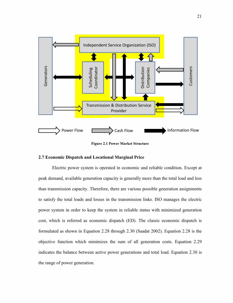
Figure 2.1 shows a power market structure. Electric power propagates from
generators to customers through a transmission and distribution (T&D) service provider.
On the other hand, cash is channeled in the opposite direction, from customers to
generators and T&D providers. Information, including power price and amount of power
supply and demand, is exchanged among the entities. In a power market, PEV
infrastructure will be both generator and customer in that PEV infrastructure can be
operated both in V2G and in G2V.
1 Electric Reliability Council of Texas
21
Figure 2.1 Power Market Structure
2.7 Economic Dispatch and Locational Marginal Price
Electric power system is operated in economic and reliable condition. Except at
peak demand, available generation capacity is generally more than the total load and less
than transmission capacity. Therefore, there are various possible generation assignments
to satisfy the total loads and losses in the transmission links. ISO manages the electric
power system in order to keep the system in reliable status with minimized generation
cost, which is referred as economic dispatch (ED). The classic economic dispatch is
formulated as shown in Equation 2.28 through 2.30 (Saadat 2002). Equation 2.28 is the
objective function which minimizes the sum of all generation costs. Equation 2.29
indicates the balance between active power generations and total load. Equation 2.30 is
the range of power generation.
Ge
ne
rato
rs
Transmission & Distribution Service Provider
Cu
sto
mer
s
Dis
trib
uti
on
C
om
pan
ies
Independent Service Organization (ISO)
Sch
edu
ling
Co
ord
inat
or
Power Flow Cash Flow Information Flow
22
1
minm
i gi
i
f C P
(2.28)
1
. .m
gi L
i
s t P P
(2.29)
min max 1, ,gi gi giP P P i m
(2.30)
where, iC is the cost function of generator. giP is the real power generation of the i
th generator. mingiP and
maxgiP are real power limits of the i th generator. m is the number
of generators. LP is the fixed load demand.
Settlement price for ancillary service and transmission congestion cost are
estimated in terms of locational marginal price (LMP) that is the cost of providing the
next increment of demand at a specific node. Different LMPs between buses are
generally caused by power system operating conditions, such as transmission system,
generation, and load. Ott (2003) presented mathematical LMP formulations that are
utilized in PJM market as shown in Equation 2.31 through 2.35. Comparing classic
economic dispatch, the equations for LMP consider transmission system configurations
which are expressed as a shift factor in equations. Shift factors are a measure of the
change in power flow on the constraint’s monitored elements for a unit change in
megawatt injection at a bus and a corresponding unit change in megawatt withdrawal at
the reference bus. Through the shift factors, electric power flow on transmission
constraints can be calculated.
23
1 1
minm n
i i j Lj
i j
Z C P C P
(2.31)
1 1
. . 0m n
i Lj
i j
s t P P
(2.32)
min maxi i iP P P
(2.33)
min maxLj Lj LjP P P
(2.34)
0ik i jk LjA P D P
(2.35)
where, ikA is the matrix of shift factors for generation bus on the binding transmission
constraints k . jkD is the matrix of shift factors for load bus on the binding transmission
constraints k .
LMP at a particular location is the sum of the marginal price of generation at the
reference bus and the marginal congestion price at the location associated with the
various binding transmission constraints. Formulation for LMP is as follows:
i ik kLMP A SP (2.36)
where, is marginal price of generation at the reference bus. kSP is shadow price of
constraint k .
PEV parking building will buy or sell electricity as charging station and
distributed generator. In this situation, LMP is used as clearing price for trading an
electric power.
24
2.8 Summary
The literature review provided fundamental equations that are necessary to
develop new problems. This section also presented the necessary background for
creating a new facility location problem that can explain the interactions between
transportation and electric power systems and a new charging station installation
problem that considers uncertainty in parameters. In the following sections, the basic
problems from the literature are reformulated and adjusted for developing the new
models that can help PEV parking building developers and managers make optimal
decisions.
25
3. PEV PARKING BUILDING DEVELOPMENT PROBLEM*1
Unlike conventional parking buildings, PEV parking buildings can provide
charging services to users and contract with an independent system operator (ISO) to
service the grid and make a profit. This section presents a mathematical model for
finding the optimal location and operations plan for a new PEV parking building.
The revenue of PEV infrastructure project is closely related to the number of
parked PEVs. The location of a PEV parking building and the amount of (dis)incentive
(fee or rebate) are important factors when drivers decide where to park. Details of the
problem description will be discussed in the first section of this section. In the second
section, a mathematical model for a PEV parking building problem is formulated in the
form of a BLPP. Then, in the third section, two numerical examples are presented.
3.1 Problem Description
Commercial and public parking buildings in a central business district (CBD)
provide thousands of parking spaces for commuters and visitors. However, none of these
facilities are equipped with charging infrastructure for PEVs. In the future, PEV owners
will consider parking their vechicles in buildings that can provide charging services for
depleted vehicle batteries.
*
1 Reprinted with permission from “Smart Garage Development Problem: A Model Formulation and a
Solution Approach” by Kim, S. and Damnjanovic, I., 2011. Journal of Infrastructure Systems, Copyright
2011 by ASCE.

26
A PEV parking building represents an interface between a transportation network
and an electric power system. Figure 3.1 shows a PEV parking building acting as the
interface between the two networks: it provides charging services for PEV drivers,
which is a G2V operation; as well as ancillary services for an electricity power network,
which is a V2G operation. To facilitate these operations, a PEV parking building needs
to communicate with an ISO to obtain prices and to identify the amount of available
electricity to provide.
Figure 3.1 Roles of PEV Parking Building
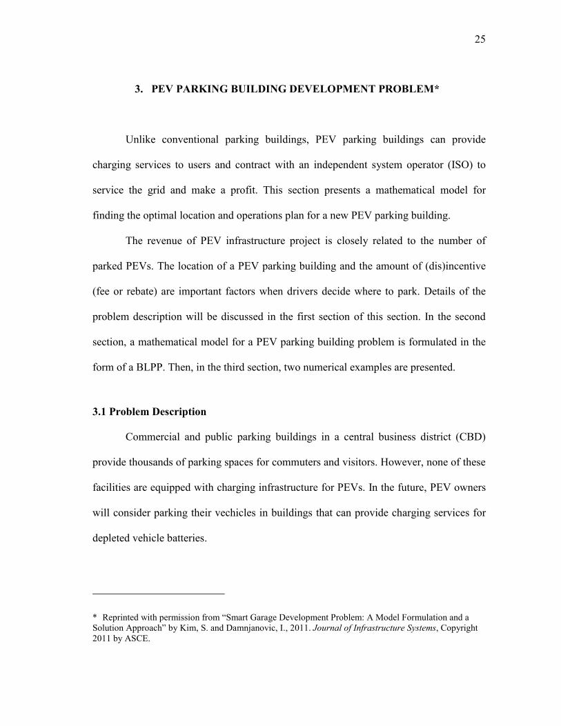
Figure 3.2 shows a simple transportation network with a PEV parking building.
When a new PEV parking building is constructed, PEV drivers have two options:
proceed to the final destination directly, or park at the PEV parking building and walk to
the destination. Drivers in transportation networks select a parking garage based on
multiple factors. These include cost of parking, congestion on links, walking distance,
and others. In this problem, the location of the PEV parking building and the fee
27
structure are considered decision variables (i.e. under control of the parking garage
developer).
Figure 3.2 Simple Transportation Network with PEV Parking Building
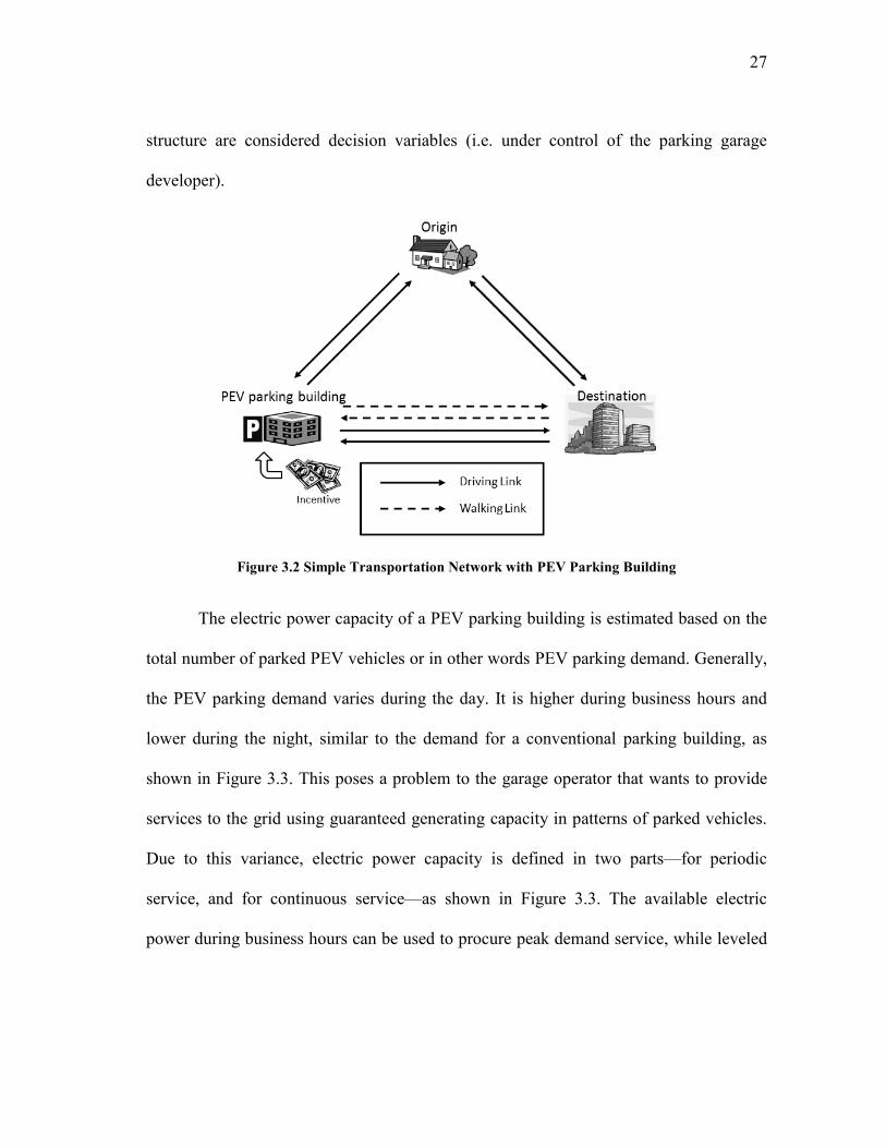
The electric power capacity of a PEV parking building is estimated based on the
total number of parked PEV vehicles or in other words PEV parking demand. Generally,
the PEV parking demand varies during the day. It is higher during business hours and
lower during the night, similar to the demand for a conventional parking building, as
shown in Figure 3.3. This poses a problem to the garage operator that wants to provide
services to the grid using guaranteed generating capacity in patterns of parked vehicles.
Due to this variance, electric power capacity is defined in two parts—for periodic
service, and for continuous service—as shown in Figure 3.3. The available electric
power during business hours can be used to procure peak demand service, while leveled
28
constant capacity (0-24hr) can be used to provide regulation service in the V2G mode of
operation.
Figure 3.3 Example of Demand of PEV Parking Building for One Day
To standardize the proposed problems, four key assumptions are considered:
When choosing travel paths, users follow the user equilibrium principle
(Wardrop 1952). Wardrop’s first principle implies that drivers choose the
routes that minimize the travel cost. The user equilibrium is obtained when no
driver can find a lower transportation cost as a result of changing his or her
route choice.
The parking building users return from the destination to the origin directly.
For simplicity, trip chaining is not considered.
The time interval is defined as one hour and all trips occur within this time
interval. Traffic flow from the origin to the destination and from the destination

29
to the origin is generated every hour, and parking duration is defined in the unit
of one hour.
Penetration (or adoption) rate of PEVs is constant. Ratio of PEVs to all
vehicles of traffic flow would be different every hour and on every link, but,
for simplicity, the ratio is assumed as being constant.
3.2 The Model
Consider a directed network ,G N A of N nodes and A links, where set A
consists of two subsets of links: driving (roadway) and walking (sidewalk) links, DA
and WA , respectively. The network includes k origin-destination (O-D) pairs ,i ir s , ir ,
is N , 1,...,i k , and mode transfer nodes.
The PEV parking building problem in this study was formulated to determine the
optimal location and (dis)incentive structure on a pre-specified link. The PEV parking
building problem has two level problems. The notations of the PEV parking building
problem are as follows:
Sets
DA = the set of driving links in the O-D trip
WA = the set of walking links in the O-D trip
J = the set of path of the ICEV
K = the set of path of the PEV
N = the set of nodes
W = the set of path of non-users of the PEV parking building
Y = the set of path of users of the PEV parking building

30
Parameters
ac = the capacity of the driving link
bc = the capacity of the walking link
disE
= the total energy dispatched over the contract period
f = the parking fee at the conventional parking building
f = the parking fee at the PEV parking building
I = the upper limit of incentive ( i )
L = the upper limit of distance ( l )
P = the power limited by a vehicle’s stored energy
capp = the capacity price
conP
= the contracted capacity (MW)
d cR = the dispatch-to-contract ratio
as = the average speed of cars
bs = the average speed of pedestrians
cont
= the duration of the contract
U
= the upper limit of parking hours ( u )
ˆhZ
= the forecast power price
= the incentive parameter
,
rs
a j = the indicator variable—1 if link a is on path j of ICEV connecting
O-D pair r - s , 0 otherwise
= the power extraction ratio
= the ratio of PEVs to all vehicles
Variables
hd
= the PEV parking demand on time h
rs
j hf = the flow on path j of ICEV connecting O-D pair r - s on time h
i
= the incentive provided by the PEV parking building
l
= the distance between the PEV parking building and destination
rs
j hq = the trip rate of ICEV connecting O-D pair r - s on time h
PFr = the revenue from the parking fee
PHr = the revenue from the peak hour service
RSr = the revenue from the regulation service
Totalr = the total revenue

31
at = the driving link cost function
bt = the walking link cost function
a hx = the link flows on driving links at time h
u
b hx = the link flows on walking links at time h and with u parking hours
The PEV parking building problem is formulated as follows:
,
max , , , ,Total PF RS PHl i
r l i r l i r l i r l i (3.1)
. . 0s t l L
(3.2)
0 i I (3.3)
1 1
1 2
,N N N
u u u
h b b b Wh h h nu u u n
d l i x x x b A
(3.4)
0 0
min , , , ,a b
D W
x x
a b hhA A
t l i d t l i d
(3.5)
. . ,rs rs
j jh hj
s t f q r N s N (3.6)
,rs rs
k kh hk
f q r N s N (3.7)
,sr sr
w wh hw
f q r N s N (3.8)
,sr sr
y yh hy
f q r N s N (3.9)
, , , 0 , ,
, ,
rs rs sr sr
j k w yh h h hf f f f r N s N j J
k K w W y Y
(3.10)
, ,
, ,
rs rs rs rs
a j a j k a kh h hr s j r s k
sr sr sr sr
w a w y a yh hr s w r s y
D
x f f
f f
a A
(3.11)
32
, ,
rs rs sr sr
b k b k y b y Wh h hr s k r s y
x f f b A (3.12)
The upper-level objective function specified in Equation 3.1 consists of three
revenue components: parking fee (disincentive), regulation service fee, and peak demand
service fee. Equations 3.2 and 3.3 define the location and incentive decision space.
Equation 3.4 defines the PEV parking demand based on the results from the user
equilibrium problem. The lower-level problem is the user equilibrium problem with two
user classes (PEV and ICEV), time-dependent trip rates, and walking link costs.
3.2.1 Lower-Level Problem
Construction of a PEV parking building changes the topology of a transportation
network and drivers’ behaviors. As it represents an additional node, the existing driving
and walking link cost functions can be modified to account for changes in network
topology and the link cost. The modified driving and walking link cost functions are
discussed in the Modified Link Cost Functions section.
O-D trip rates and parking hours are considered deterministic. Destination-origin
(D-O) trip rates are calculated from the result of the O-D assignment problem and
assumed parking hours. There are two types of D-O trip rates: “proceed to origin directly”
and “walk to the PEV parking building and drive to origin.” Here, D-O trip rate of
“proceed to origin directly” is derived from O-D trip rate of ICEV and PEV which do
not park at PEV parking building, while D-O trip rate of “walk to the PEV parking
building and drive to origin” is calculated from O-D trip rate of PEV which park at PEV
parking building. The details for trip rates are discussed in the Trip Rates section.
33
Modified Link Cost Functions
A Bureau of Public Roads (BPR 1964) function has been widely used by
researchers and engineers to model travel time/cost on roadway links. A similar function
was developed by Fox and Associates (1994) for modeling pedestrian travel on walking
links. Free-flow driving and walking time is derived from the lengths of the driving and
walking links ( al and bl ) and the average speeds of vehicles and pedestrians ( as and bs ).
Equations 3.13 and 3.14 present modified link cost functions, where the walking link
cost function in Equation 3.14 includes the effect incentive ( i ) on the travel time.
1
a
a aa a D
a a
l xt a A
s c
(3.13)
b
b bb b W
b b
l xt i b A
s c
(3.14)
where, the quantities and are model parameters.
In Equation 3.14, represents a cost parameter that transfer walking time into
cost function. For example, an incentive parameter of 20 means that people will price
20 minutes of walk as $1. This incentive parameter is affected by the walkability of the
walking links. For example, people prefer to walk in urban area links, which means the
incentive parameter increases with an increase in the quality of walking links. Several
studies (Southworth 2005; Litman 2003; Hess et al. 1999) identified important attributes
for the design of a pedestrian network, such as safety, quality of walking path, and
connectivity of paths. Landis (2001) developed a mathematical model to measure
34
pedestrian level of service (LOS) using statistical methods, while Hoogendoorn and
Bovy (2004) developed a mathematical theory for pedestrian behavior in respect to
walking cost and utility.
Trip Rates
This study considered bi-direction trips: O-D and D-O. The total O-D trip rates
(rs
Totalq ) were divided into two categories: the trip rates of ICEVs ( jq ) and the trip rates
of PEVs ( kq ) defined by the penetration rate of PEVs ( ). The trip rates were assumed
to be generated in intervals of one hour and are defined as follows:
1
,
rs rs rs rs rs
Total j k Total Totalh h h h hq q q q q
r N s N
(3.15)
While total O-D trip rates are divided by types of vehicles, the total D-O trip
rates (rs
Totalq ) are divided by whether or not drivers use the PEV parking building. Hence,
there are two D-O trip rates: the rate for the vehicles that have not parked at the PEV
parking building (sr
wq ) and the rate for the vehicles that have (sr
yq ). The D-O trip rates
are defined as follows:
,sr sr sr
Total w yh h hq q q r N s N (3.16)
The D-O trip rates are determined from the results of the previous O-D
assignment problem. That is, drivers assigned to a PEV parking building in the previous
O-D trips should walk back to the parking building in the D-O trip, and drivers assigned

35
to a conventional parking garage in previous O-D trips should return to their origins
directly in the D-O trip.
The link flows on WA are composed of drivers who park for different parking
hours, which is defined in Equation 3.17. The link flows b hx are part of rs
k hq and
are obtained from the assignment problem.
1 2 U
b b b b Wh h h hx x x x b A (3.17)
D-O trip rates, sr
wq and sr
yq , are calculated based on link flows b hx . Trip rate
sr
yq is derived from the pedestrian flows, bx , of PEV drivers who parked their cars in the
PEV parking building. As discussed above, bx could be divided into u
bx ’s, depending
on parking hours, u . The parking hours, u , should be less than or equal to U . Drivers
who have parked their vehicles for specific hours will leave the parking building after
their stay at the destination node expires. Therefore, 1
sr
y hq
is defined as follows:
1 1
1
, ,h
usr
y b Wh h uu
q x b A r N s N
(3.18)
Finally 1
sr
w hq
is computed by subtracting
1
sr
y hq
from D-O trip rates. It is
defined as follows:
1 1 1 1
1
, ,
hu u u
sr rs rs
w j k bh h u h u h uu
W
q q q x
b A r N s N
(3.19)
36
3.2.2 Upper-Level Problem
Kempton and Tomic (2005b) proposed a business model that can be applied to
V2G technologies. The revenue from V2G technologies can be obtained from three
types of services the garage provides to the grid: peak power, spinning reserve, and
regulation. Much like in Kempton and Tomic’s (2005b) model, the manager of a PEV
parking building has an option to partially discharge the stored power from parked PEV
batteries during parking hours. The total amount of available power is dependent on the
number of parked PEVs, or, in other words, on the PEV parking demand ( hd ).
As previously mentioned, this study considered an upper-level objective based on
three revenue components: the parking fee, the regulation service, and the peak hour
service. The incentive that the PEV parking building could provide to the users can be
considered as a cost, or a negative value of the parking fee. Hence, in an upper-level
objective, there is a tradeoff between the parking fee and the cost of attracting more
PEVs to park and get the value from ancillary service fees. When a PEV parking
building is constructed at location l and provides incentive i to users, the revenue model
from the parking fee is defined as follows:
24
1
, ,PF h
h
r l i d l i f
(3.20)
where, f is the parking fee at a PEV parking building and is the difference between the
parking fee at a conventional parking building ( f ) and the incentive provided by a PEV
parking building ( i ).

37
In addition to the revenue from parking fees, the garage operator receives
revenue from V2G operations. Utilizing the PEV in the PEV parking building, the
operator contracts with an aggregator (or independent system operator) to provide power
regulation storage and peak hour services.
The regulation service—one of the key ancillary services—corrects unintended
fluctuations of power generation in order to meet a load demand. If a load demand
exceeds power generation, PEVs discharge power from the battery, and if power
generation meets a load demand, when battery capacity is abundant, PEVs charge power
from the power grid. The PEV parking building can provide regulation service for 24
hours at the level of * ,d l i , as shown in Figure 3.3. Kempton and Tomic (2005b)
suggested a revenue model for regulation service as follows:
24
*
1
ˆ, ,RS cap d c h
h
r l i d l i p P P R Z
(3.21)
where, P is the power limited by the vehicle’s stored energy, * ,d l i is the minimum
amount of vehicles for 24 hours, ˆhZ is the forecast power price, capp is the capacity
price, and d cR is the dispatch-to-contract ratio, as defined below:
disd c
con con
ER
P t (3.22)
where, disE is the total energy dispatched over the contract period, conP is the contracted
capacity (MW), and cont is the duration of the contract.
38
The peak hour demand market is another source of revenue for the operator of a
PEV parking building. The extracted power from the PEVs parked during the day can
provide electric power, with the PEVs basically functioning as a distributed generator.
The manager of the PEV parking building can contract with the ISO to sell power for a
specific period. In this study, the specific period was defined as 8:00 a.m. to 8:00 p.m.,
when demand for the PEV parking building is high. The PEV parking building can
extract power up to ***d , which would be the point that the battery in a PEV is drained.
Therefore, defining a proper power extraction ratio ( ) is essential. The revenue model
for the peak hour services is defined as follows:
20
**
8
ˆ, ,PH h
h
r l i P d l i Z
(3.23)
where, ** *** *, , ,d l i d l i d l i and *** ,d l i is the maximum amount of
vehicles between 8:00 a.m. and 8:00 p.m.
3.3 Computational Study
Numerical examples to illustrate the application of the developed bilevel PEV
parking building problem are presented next. In the first section, a simple network
structure is considered to investigate system behavior when the effects can be isolated.
In the next section, a large network is considered to capture realistic situations.
39
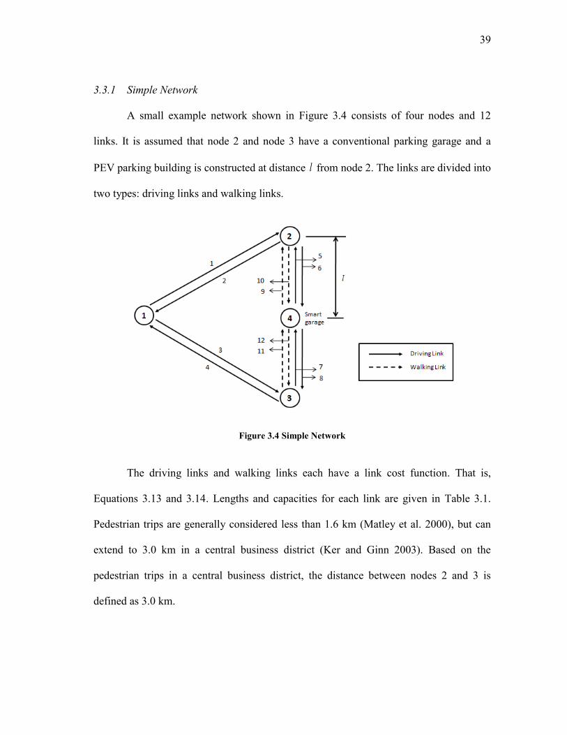
3.3.1 Simple Network
A small example network shown in Figure 3.4 consists of four nodes and 12
links. It is assumed that node 2 and node 3 have a conventional parking garage and a
PEV parking building is constructed at distance l from node 2. The links are divided into
two types: driving links and walking links.
Figure 3.4 Simple Network
The driving links and walking links each have a link cost function. That is,
Equations 3.13 and 3.14. Lengths and capacities for each link are given in Table 3.1.
Pedestrian trips are generally considered less than 1.6 km (Matley et al. 2000), but can
extend to 3.0 km in a central business district (Ker and Ginn 2003). Based on the
pedestrian trips in a central business district, the distance between nodes 2 and 3 is
defined as 3.0 km.
40
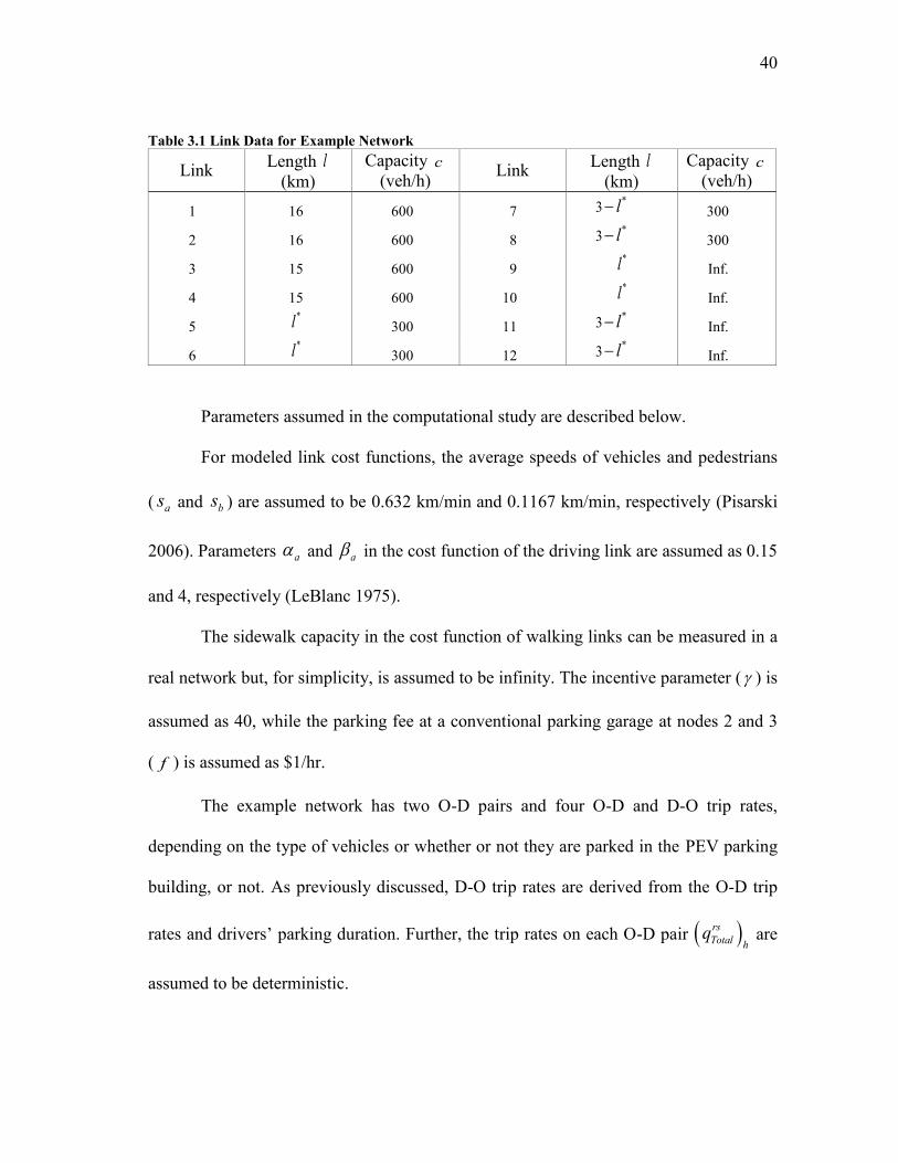
Table 3.1 Link Data for Example Network
Link Length l
(km)
Capacity c
(veh/h) Link
Length l
(km)
Capacity c
(veh/h)
1 16 600 7 *
3 l
300
2 16 600 8 *
3 l
300
3 15 600 9 *l
Inf.
4 15 600 10 *l
Inf.
5 *l
300 11 *
3 l
Inf.
6 *l
300 12 *
3 l
Inf.
Parameters assumed in the computational study are described below.
For modeled link cost functions, the average speeds of vehicles and pedestrians
( as and bs ) are assumed to be 0.632 km/min and 0.1167 km/min, respectively (Pisarski
2006). Parameters a and a in the cost function of the driving link are assumed as 0.15
and 4, respectively (LeBlanc 1975).
The sidewalk capacity in the cost function of walking links can be measured in a
real network but, for simplicity, is assumed to be infinity. The incentive parameter ( ) is
assumed as 40, while the parking fee at a conventional parking garage at nodes 2 and 3
( f ) is assumed as $1/hr.
The example network has two O-D pairs and four O-D and D-O trip rates,
depending on the type of vehicles or whether or not they are parked in the PEV parking
building, or not. As previously discussed, D-O trip rates are derived from the O-D trip
rates and drivers’ parking duration. Further, the trip rates on each O-D pair rs
Total hq are
assumed to be deterministic.
41
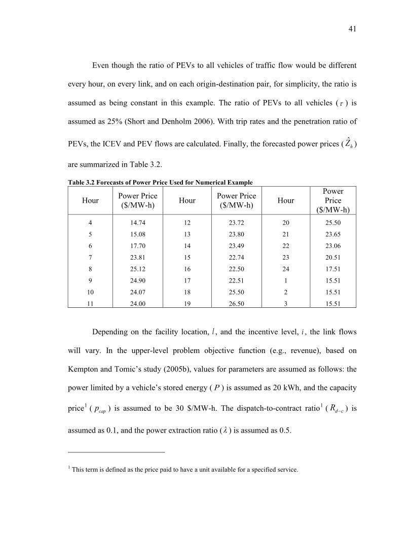
Even though the ratio of PEVs to all vehicles of traffic flow would be different
every hour, on every link, and on each origin-destination pair, for simplicity, the ratio is
assumed as being constant in this example. The ratio of PEVs to all vehicles ( ) is
assumed as 25% (Short and Denholm 2006). With trip rates and the penetration ratio of
PEVs, the ICEV and PEV flows are calculated. Finally, the forecasted power prices ( ˆhZ )
are summarized in Table 3.2.
Table 3.2 Forecasts of Power Price Used for Numerical Example
Hour Power Price
($/MW-h) Hour
Power Price
($/MW-h) Hour
Power
Price
($/MW-h)
4
5
6
7
8
9
10
11
14.74
15.08
17.70
23.81
25.12
24.90
24.07
24.00
12
13
14
15
16
17
18
19
23.72
23.80
23.49
22.74
22.50
22.51
25.50
26.50
20
21
22
23
24
1
2
3
25.50
23.65
23.06
20.51
17.51
15.51
15.51
15.51
Depending on the facility location, l , and the incentive level, i , the link flows
will vary. In the upper-level problem objective function (e.g., revenue), based on
Kempton and Tomic’s study (2005b), values for parameters are assumed as follows: the
power limited by a vehicle’s stored energy ( P ) is assumed as 20 kWh, and the capacity
price1 ( capp ) is assumed to be 30 $/MW-h. The dispatch-to-contract ratio
1 ( d cR ) is
assumed as 0.1, and the power extraction ratio ( ) is assumed as 0.5.
1 This term is defined as the price paid to have a unit available for a specified service.

42
Results
Figure 3.5 shows the demand patterns for the PEV parking building ( hd )
depending on l and i . In the legend, the first value in the parentheses indicates the
amount of incentive in ‘$’ and the second value indicates the location of the PEV
parking building in ‘km’. The various garage demand scenarios were calculated by using
combinations of the location and the incentive. It can be observed from the figure that as
the incentive increases and the optimal location is centered between the two nodes, the
PEV parking demand increases as well. This result shows that PEV parking demand will
be the greatest, when PEV parking building is constructed where PEV drivers can move
with minimizing their travel costs. With more PEV parking demand, parking building
developer can make more profit by providing charging service and utilizing electric
power stored in PEVs.
To find optimal solution, PEV parking development model in the form of bilevel
problem will have to be solved. As a bilevel nonlinear programming problem is an NP-
hard problem (Hansen et al. 1992), a genetic algorithm (GA) was utilized. A genetic
algorithm is a method of searching the fitness landscape for a highly fit (i.e. optimal)
solution. This algorithm is inspired by evolutionary biology, as the population (solution)
is increasingly better adapted, much like in the evolutionary process (Mitchell 1998).
The simple form of a genetic algorithm typically consists of three types of operators,
1 This term is defined for that actual energy dispatched for regulation is some fraction of the total power
available and contracted for.
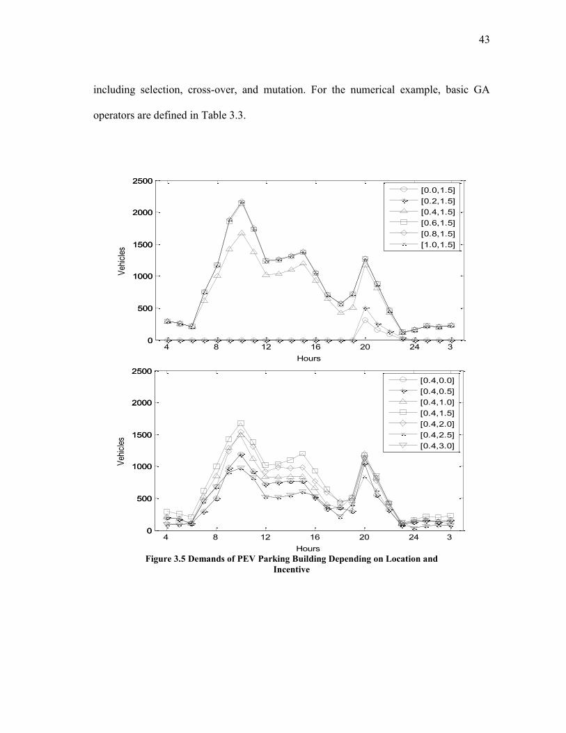
43
including selection, cross-over, and mutation. For the numerical example, basic GA
operators are defined in Table 3.3.
Figure 3.5 Demands of PEV Parking Building Depending on Location and
Incentive
4 8 12 16 20 24 3 0
500
1000
1500
2000
2500
0
500
1000
1500
2000
2500
Hours
Veh
icle
s
[0.0,1.5]
[0.2,1.5]
[0.4,1.5]
[0.6,1.5]
[0.8,1.5]
[1.0,1.5]
4 8 12 16 20 24 3 0
500
1000
1500
2000
2500
0
500
1000
1500
2000
2500
Hours
Veh
icle
s
[0.4,0.0]
[0.4,0.5]
[0.4,1.0]
[0.4,1.5]
[0.4,2.0]
[0.4,2.5]
[0.4,3.0]
4 8 12 16 20 24 3 0
500
1000
1500
2000
2500
0
500
1000
1500
2000
2500
Hours
Veh
icle
s
[0.0,1.5]
[0.2,1.5]
[0.4,1.5]
[0.6,1.5]
[0.8,1.5]
[1.0,1.5]
4 8 12 16 20 24 3 0
500
1000
1500
2000
2500
0
500
1000
1500
2000
2500
Hours
Veh
icle
s
[0.4,0.0]
[0.4,0.5]
[0.4,1.0]
[0.4,1.5]
[0.4,2.0]
[0.4,2.5]
[0.4,3.0]
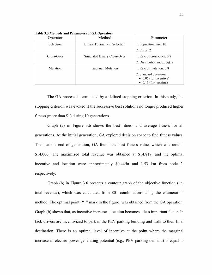
44
Table 3.3 Methods and Parameters of GA Operators
Operator Method Parameter
Selection Binary Tournament Selection 1. Population size: 10
2. Elites: 2
Cross-Over Simulated Binary Cross-Over 1. Rate of cross-over: 0.8
2. Distribution index (η): 2
Mutation Gaussian Mutation 1. Rate of mutation: 0.8
2. Standard deviation:
0.05 (for incentive)
0.15 (for location)
The GA process is terminated by a defined stopping criterion. In this study, the
stopping criterion was evoked if the successive best solutions no longer produced higher
fitness (more than $1) during 10 generations.
Graph (a) in Figure 3.6 shows the best fitness and average fitness for all
generations. At the initial generation, GA explored decision space to find fitness values.
Then, at the end of generation, GA found the best fitness value, which was around
$14,000. The maximized total revenue was obtained at $14,817, and the optimal
incentive and location were approximately $0.44/hr and 1.53 km from node 2,
respectively.
Graph (b) in Figure 3.6 presents a contour graph of the objective function (i.e.
total revenue), which was calculated from 801 combinations using the enumeration
method. The optimal point (“+” mark in the figure) was obtained from the GA operation.
Graph (b) shows that, as incentive increases, location becomes a less important factor. In
fact, drivers are incentivized to park in the PEV parking building and walk to their final
destination. There is an optimal level of incentive at the point where the marginal
increase in electric power generating potential (e.g., PEV parking demand) is equal to
45
the marginal opportunity cost of charging for parking. For example, if developer
provides more incentive, PEV parking demand will be increased, but total revenue could
be decreased due to excessive incentive. Therefore, finding optimal incentive is very
important to maximize a profit.
(a) (b) Figure 3.6 Fitness and Contour Graph for Total Revenue
Sensitivity Analysis
The suggested model is based on a number of empirical variables and
parameters, including the battery limitation (i.e., power limited by the vehicle’s stored
energy), ratio of extraction, and trip rates. As the value of these parameters is largely
uncertain, a sensitivity analysis was conducted to understand the extent of their marginal
influences.
Figure 3.7 shows the results of the sensitivity analysis. The penetration rate of a
PEV ( ) and the power limited by the vehicle’s stored energy ( P ) have the most
significant effect on the total revenue when contrasted with the other parameters. The
total revenue is sensitive to changes of trip rate from node 1 to node 2 much more than

46
the changes of trip rate from node 1 to node 3. The difference of sensitivity comes from
the volume of trip rate.
Figure 3.7 Results of Sensitivity Analysis
The sensitivity analysis also showed that the change of trip rate and incentive
parameter could affect the optimal location and incentive. The optimal location is
located close to the node where a greater trip rate is allocated, and the optimal incentive
decreases as the location of the PEV parking building moves closer to the node with the
conventional parking garage. Similar to the sensitivity analysis for the total revenue, the
trip rate with the higher traffic flow has more influence on the total revenue.
The results of the sensitivity analysis indicate important implications for PEV
parking building management. First, in the planning stage, the developer of the PEV
parking building should consider long-term changes in future traffic flow and locate a
PEV parking building closer to the node with the highest destination trip rate. Second, to
47
attract more parking users, the operator needs to consider the walkability of walking
links. For example, even if the manager of the PEV parking building provides much
incentive, pedestrians do not want to walk through a dangerous area with poor
walkability. Third, the operator of the PEV parking building can control the demand of
the PEV parking building by manipulating the incentive structure (parking fee). For
instance, when there is an excessive demand for a PEV parking building, the operator
can readjust the incentive and reduce the demand of the PEV parking building, or vice
versa. In other words, the operator should decrease the cost of parking fee to the level
when total marginal benefits from V2G operations equal to the opportunity cost from
parking service.
3.3.2 Large Network
PEV parking building model is applied next to larger and more realistic network,
Sioux Falls network in Figure 3.8. The network consists of 24 nodes, 38 driving bi-
directional links and 38 walking bi-directional links. Trip rates between nodes and
parameters for link cost function are given in APPENDIX II and APPENDIX III,
respectively. The network, trip rates, and parameters are referred from LeBlanc’s work
(1975). The values of other parameters, including average speed of vehicles and
pedestrians, parking fee in conventional parking building, and electric power prices, are
assumed equal to the case on the simple network used in the previous section.
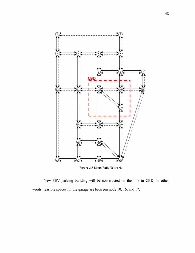
48
Figure 3.8 Sioux Falls Network
New PEV parking building will be constructed on the link in CBD. In other
words, feasible spaces for the garage are between node 10, 16, and 17.
49
Results
Like in a simple network, the genetic algorithm approach is utilized to find
optimal solution. The GA operators and methods are the same as in the simple network
(see Table 3.3), but some parameters are defined differently; distribution index (η) is
defined as 1.5, and rate of mutation is defined as 0.2. Standard deviation for optimal
location is defined as ‘0.05×length of the link’, while standard deviation for incentive is
defined as ‘0.05×1’.
Figure 3.9 shows the best fitness and average fitness for all generations. GA
found the best fitness value, which was around $1,550,000. The maximized total revenue
was obtained at $1,547,700. The optimal incentive was approximately $0.24/hr, and
optimal location of PEV parking building was 0.045 km from node 10 on the link
between node 10 and node 16.
Figure 3.9 Fitness Graph for Total Revenue
50
The result confirms that optimal location is close to the node where the greatest
trip rate is located. Among three nodes in CBD, node 10 has the higher trip rate and node
16 has the second most trip rate. The optimal location of PEV parking building is not
only on the link between node 10 and node 16, but also closer to node 10.
Sensitivity Analysis
Figure 3.10 shows the results of the sensitivity analysis for large network. The
result shows that the change of trip rate has the most significant effect on the total
revenue when contrasted with the other parameters. Unlike penetration rate of a PEV in
the sensitivity analysis of simple network, the penetration rate of a PEV in the sensitivity
analysis of large network is much less sensitive, which indicates penetration rate has
more influence on small network or with less trip rate. The link capacities have the least
effect on the total revenue.
Figure 3.10 Result of Sensitivity Analysis
51
When trip rate to node 10 is reduced to the ratio of 0.2, the total revenue
decreases and the optimal location changes from the link between node 10 and node 16
to the link between node 16 and node 17. As trip rate to node 10 decreases, the optimal
location of PEV parking building moves away from node 10. This change of the optimal
location is also observed with changes in other factors, such as incentive parameter and
penetration rate of PEV. As incentive parameter and penetration rate are reduced, the
optimal location of PEV parking building is on the link between node 16 and node 17,
not on the link between node 10 and node 16.
Sensitivity analysis of the large network provides similar implications for PEV
parking building management. In a planning stage of PEV parking building project, the
developer should carefully consider future change of trip rate. The trip rate shows
significant influence on the total revenue and the location of PEV parking building. Also,
developer needs to consider walkability of walking links, which is related to incentive
parameter. Better walkability will bring more profit for developers.
3.4 Summary
This section presented a strategic model that can be used to determine the
optimal location for a PEV parking building and the optimal incentive, or parking fee
structure. Such a parking facility for PEVs represents an interface between a
transportation network and an electric power system. Hence, traffic flows and power
prices need to be considered simultaneously. In this study, a traffic assignment problem
was used to determine transportation network flow with multi-class users, time-
52
dependent trip rates, and walking link costs. The results of the model show that demand
for a PEV parking building is highly sensitive to selected location and incentive
structure. Finally, the model was formulated as a bilevel problem with an upper
objective composed from three revenue components: the parking fee, the peak hour
service, and the regulation service.
Some fundamental insights into how the results in this study can be applied on
real networks are provided. First, the maximum trip rate has a significant effect on the
optimal location and incentive of a PEV parking building. Second, the walkability of
walking links is an important factor in determining the optimal location and incentive
and is related to the study of incentives. Sensitivity analysis shows that PEV parking
demand is highly influenced by poor walkability, or lower incentive parameters.
53
4. IMPACT OF PEV ON ELECTRICITY NETWORK
In the future, PEV parking facilities could be an important place for exchange of
electric power. Parking building developers could have an opportunity to gain revenue
not only from the parking fees and charging services, but also by acting as an aggregator
in electricity markets. A PEV parking building uses electricity for charging services and
generates electricity from PEV batteries for ancillary services. This section investigates
the impact of PEVs on traffic flow and micro-level power system configurations, such as
a nodal area, from a parking garage developer’s perspective. The model in this section is
an extension of the previous PEV parking development model in which market
electricity price is considered as a parameter.
The next section will present an overview of the problem and the key
assumptions. Section 4.2 presents mathematical formulations of the model. A simple
numerical example showing the impact of PEVs and the total revenue model is provided
in Section 4.3.
4.1 Problem Description
Generally, a bus1 in a power network represents the smallest unit where power
transaction is conducted. A bus could be associated with one or more nodes placed
within an operating area. Figure 4.1 shows a schematic representation of a power and a
1 A bus represents the bus bar within a piece of switchgear, motor control centers, panels or
other load points.
54
transportation network with a PEV parking building. While node 1 is within the
operating area of bus 1, node 2 and node 3 are within the operating area of bus 2.
Figure 4.1 Schematic Representation of the Networks with a PEV Parking Building
In the transportation network, both node 1 ( 1n ) and node 2 ( 2n ) have
conventional parking garages where both ICEVs and PEVs can be parked. Node 3 ( 3n )
indicates the PEV parking building where PEVs can be charged or discharged. PEV
drivers would choose a parking garage between node 2 and node 3 based on parking fare
and walking distance. In node 3, batteries in PEVs could be charged or discharged. That
is, the PEV parking building on node 3 could be a power load or generator within the
operating area of bus 2. Given this schematic representation, the developer of the PEV
55
parking building needs to make the optimal location and parking fare decisions that
would maximize the total revenue.
In this section, key assumptions are defined for clarity of the model presentation.
For the transportation network problem, the three assumptions defined in Section 3.1 are
used as well. For the electric power network problem, the following three assumptions
are defined for model formulation:
Minimum MW contract size is not considered.
Power load is the sum of the total power consumption within an operating area.
Movement of people between each operating area is accomplished only
through vehicles.
4.2 The Model
This section presents the formulation of the network design problem and power
system operations. First, the formulation of the network design problem explains how a
developer’s decision regarding location and incentives affects drivers’ travel choice and
a PEV parking demand. Second, the formulation of power system operations accounts
for the relationship between power system operating conditions and traffic flow of PEVs.
For this study, a directed transportation network ,G N A , with a set N of
nodes and a set A of links, was considered. Set A consists of two subsets of links:
driving and walking, DA and WA , respectively. The network includes k origin-
destination pairs ,i ir s , ir , is N , 1,...,i k . Furthermore, a power system network
56
with M 1 buses and L branches, ,P M B , was considered. The set of buses are
denoted by M 0,1,2, ,M , with the slack bus at bus 0, and the set of branches
connected between buses are denoted by B 1 2 Lb ,b , ,b .
4.2.1 Network Design Problem
The objective functions of network design problems for a PEV parking building
are formulated as follows, and constraints can be found in Section 3.2.
,
max , , , ,Total PF RS PHl i
r l i r l i r l i r l i (4.1)
,
max , , ,Total PF CHl i
r l i r l i r l i
(4.2)
A developer of a PEV parking building seeks to maximize profit by constructing
a parking garage using the optimal location and parking fare policy. A developer’s
decision on location ( *l ) and incentive ( *i ) affects the PEV parking demand and the
power system conditions, which then changes the developer’s revenue. This study
proposes two business models for the PEV parking building: one for the V2G mode and
another for the G2V mode. The total revenue for the V2G mode is defined as the sum of
the parking fee (disincentive), regulation service fee, and peak demand service fee, as
shown in Equation 4.1, while the total revenue for the G2V mode is the sum of the
parking fee and charging service fee, as shown in Equation 4.2. Three revenue
components, including parking fee, regulation service fee, and peak demand service fee,
57
were already defined in Section 3.2.2. Here, the fourth revenue component, the charging
service fee, is defined as follows:
24
, ,
1
ˆ,CH D SG c D SG hh hh
r l i P f P Z
(4.3)
where, ,D SGP is a power load from a PEV parking building and cf is a charging fee for
PEVs.
4.2.2 Power System Operating Conditions
Locational marginal price (LMP) is the cost of providing the next increment of
demand at a specific node (Ott 2003). Different LMPs between buses are generally
caused by power system operating conditions, such as transmission system, generation,
and load. As mentioned in assumptions, traffic flow of PEVs and movement of people
could change power system operating conditions, which results in changing LMPs on
buses. The model presented in this section addresses LMP problem based on V2G and
G2V operations of PEV parking building.
Power Generation and Load of PEV Parking Building
The amount of power generation and load of a PEV parking building is
determined by the number of parked PEVs (or PEV parking demand [ hd ]). PEV parking
demand varies depending on amount of traffic flow. Generally, the PEV parking demand
during the day is higher than at night, as seen in Figure 3.3. Based on PEV parking
demand, the effects of PEV parking demand on power generation and load are evaluated.
58
In the V2G mode, a PEV parking building provides both regulation service and
peak demand service. Regulation service corrects unintended fluctuations of power
generation in order to meet a load demand. The service could be called upon 400 times
per day as “regulation up” or “regulation down”. The regulation reserve equals around
1.5% of the peak demand in a regional area. However, in this study, it was assumed that
regulation service demand is not affected by PEV parking building. On the other hand,
for peak hour service, the manager of a PEV parking building can contract with the ISO
to sell electric power for a specific period. The manager needs to define power extraction
ratio to prevent PEV batteries from being drained out. For example, if the developer of a
PEV parking building extracts the entire electric power stored in PEVs for peak demand
service, batteries in PEVs would be drained. Therefore, it is essential to define a proper
power extraction ratio ( ).
Power generation and load from a PEV parking building, ,G SGP and ,D SGP , are
derived from available PEVs and discharging and charging rates:
**
, ,G SG hhP d l i P (4.4)
, ,D SG hhP d l i C
(4.5)
where, ** *** *, , ,h h hd l i d l i d l i , *** ,hd l i is the largest number of PEVs
between 8 a.m. and 8 p.m., * ,hd l i is the fewest number of PEVs for 24 hours, and C
is the charging rate.
59
Power Load on Buses
Population at origin and destination nodes, rpop and spop , can be expressed
based on trip rates:
,
r rh Total
rs rs sr sr
j k w yh h h h
pop pop
q q q q r s
(4.6)
,
s sh Total
rs rs sr sr
j k w yh h h h
pop pop
q q q q r s
(4.7)
where, r Totalpop is the total population in an origin node, s Total
pop is the total
population in a destination node, and is the average number of passengers. Details on
the trip rate can be found in Section 3.2.1.
Based on the current population, power load in node i , ,D iP , can be expressed as
follows:
,D i h ave hhP P pop
(4.8)
where, aveP is the daily average power consumption per person and h is the ratio of
power consumption on time h to power consumption for one day.
4.3 Computational Study
4.3.1 Simple Network
Figure 4.2 shows the following examples: (a) a transportation network with four
nodes and twelve links, and (b) a power network with three buses and three branches.
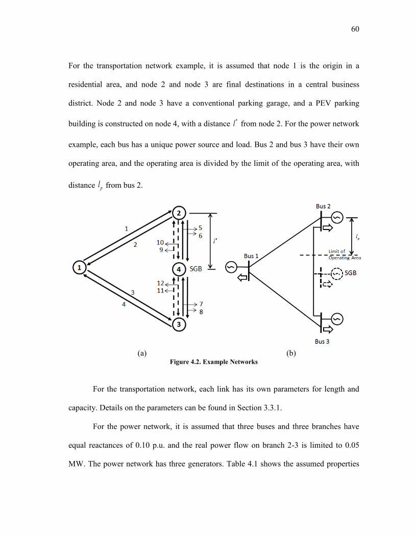
60
For the transportation network example, it is assumed that node 1 is the origin in a
residential area, and node 2 and node 3 are final destinations in a central business
district. Node 2 and node 3 have a conventional parking garage, and a PEV parking
building is constructed on node 4, with a distance *l from node 2. For the power network
example, each bus has a unique power source and load. Bus 2 and bus 3 have their own
operating area, and the operating area is divided by the limit of the operating area, with
distance pl from bus 2.
(a) (b) Figure 4.2. Example Networks
For the transportation network, each link has its own parameters for length and
capacity. Details on the parameters can be found in Section 3.3.1.
For the power network, it is assumed that three buses and three branches have
equal reactances of 0.10 p.u. and the real power flow on branch 2-3 is limited to 0.05
MW. The power network has three generators. Table 4.1 shows the assumed properties
61
of each generator. The generator offers are assumed to be in the form of a linear
function. For simplicity, voltage loss and limit are not considered (Louie and Strunz
2008).
Table 4.1 Generation Data for Example Network
Generation Bus Generation Cost
($/MW)
Max. of Generation
(MW)
Min. of
Generation
(MW)
1 20 20 0
2 25 5 0
3 30 5 0
In addition, the limit of operating area ( pl ) is assumed to be 1 km from bus 2. The
charging and discharging rates for PEVs are assumed as 1.4 kW and 20 kW, respectively
(Parks, Denholm, and Markel 2007; Kempton 2007). The initial population on the
residential area (node 1) is assumed as 15,000, and initial populations on the CBDs
(node 2 and 3) are assumed as 1,500 and 2,000. The optimal power flow problem and
locational marginal prices were computed using MatPower 3.2 (Zimmerman et al. 2011).
Results for Impact of V2G and G2V
This section presents the impact of V2G and G2V modes of new PEV parking
building on electric power network. The impact is investigated with variations of electric
power generation, load, and LMP on each bus. Generation, load, and LMP without PEV
parking building can be found in APPENDIX IV.
62
Impact of V2G
Electric power stored in PEVs is used for peak hour service in the V2G mode.
Therefore, electric power extracted from a PEV parking building reduces a power load
from 8 a.m. to 8 p.m. Figure 4.3 and Figure 4.4 show load and generation on each bus. In
the figure’s legend, the first value in the parentheses indicates the amount of incentive,
and the second value indicates the location of the PEV parking building.
Depending on the developer’s decision, the PEV parking building would be
located either within the operating area of bus 2, or bus 3. In Figure 4.3(b), the asterisk
(*) and diamond (◇) lines indicate that the PEV parking building is constructed within
the operating area of bus 2 and generates electric power. Therefore, the asterisk and
diamond lines are below the top line due to the electric power generation from the PEV
parking building. On the other hand, the load on bus 1, as seen in Figure 4.3(a), remains
unaffected because the PEV parking building is not located within the operating area of
bus 1.
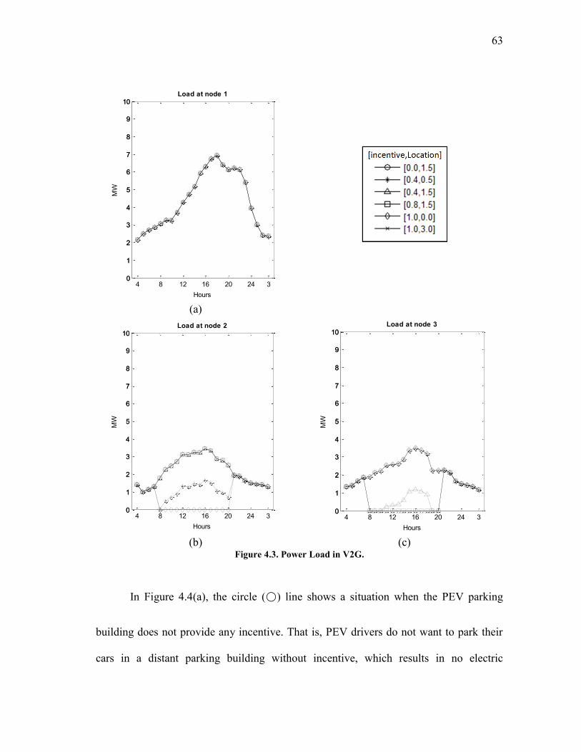
63
(a)
(b) (c)
Figure 4.3. Power Load in V2G.
In Figure 4.4(a), the circle (○) line shows a situation when the PEV parking
building does not provide any incentive. That is, PEV drivers do not want to park their
cars in a distant parking building without incentive, which results in no electric
4 8 12 16 20 24 30
1
2
3
4
5
6
7
8
9
10
0
1
2
3
4
5
6
7
8
9
10Load at node 1
Hours
MW
4 8 12 16 20 24 30
1
2
3
4
5
6
7
8
9
10
0
1
2
3
4
5
6
7
8
9
10Load at node 2
HoursM
W
4 8 12 16 20 24 30
1
2
3
4
5
6
7
8
9
10
0
1
2
3
4
5
6
7
8
9
10Load at node 3
Hours
MW
4 8 12 16 20 24 30
1
2
3
4
5
6
7
8
9
10
0
1
2
3
4
5
6
7
8
9
10Load at node 1
Hours
MW
4 8 12 16 20 24 30
1
2
3
4
5
6
7
8
9
10
0
1
2
3
4
5
6
7
8
9
10Load at node 2
Hours
MW
4 8 12 16 20 24 30
1
2
3
4
5
6
7
8
9
10
0
1
2
3
4
5
6
7
8
9
10Load at node 3
Hours
MW
4 8 12 16 20 24 30
1
2
3
4
5
6
7
8
9
10
0
1
2
3
4
5
6
7
8
9
10Load at node 1
Hours
MW
4 8 12 16 20 24 30
1
2
3
4
5
6
7
8
9
10
0
1
2
3
4
5
6
7
8
9
10Load at node 2
Hours
MW
4 8 12 16 20 24 30
1
2
3
4
5
6
7
8
9
10
0
1
2
3
4
5
6
7
8
9
10Load at node 3
Hours
MW
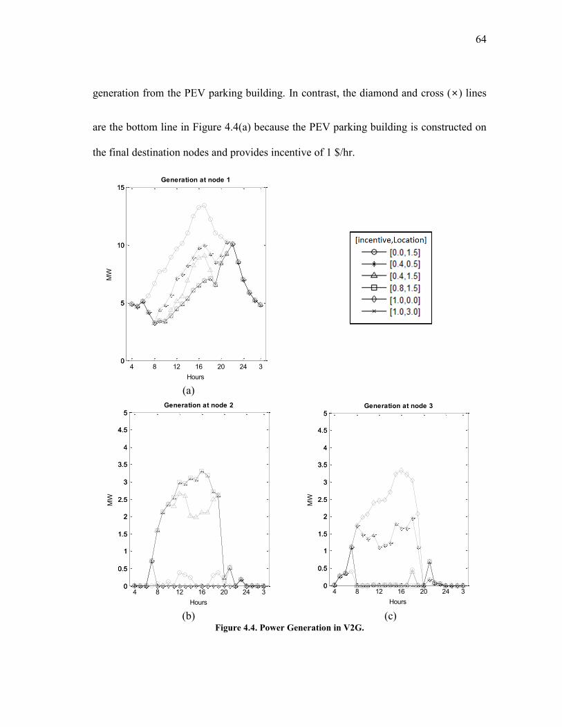
64
generation from the PEV parking building. In contrast, the diamond and cross (×) lines
are the bottom line in Figure 4.4(a) because the PEV parking building is constructed on
the final destination nodes and provides incentive of 1 $/hr.
(a)
(b) (c)
Figure 4.4. Power Generation in V2G.
4 8 12 16 20 24 30
5
10
15
0
5
10
15Generation at node 1
Hours
MW
4 8 12 16 20 24 30
0.5
1
1.5
2
2.5
3
3.5
4
4.5
5
0
0.5
1
1.5
2
2.5
3
3.5
4
4.5
5Generation at node 2
Hours
MW
4 8 12 16 20 24 30
0.5
1
1.5
2
2.5
3
3.5
4
4.5
5
0
0.5
1
1.5
2
2.5
3
3.5
4
4.5
5Generation at node 3
Hours
MW
4 8 12 16 20 24 30
5
10
15
0
5
10
15Generation at node 1
Hours
MW
4 8 12 16 20 24 30
0.5
1
1.5
2
2.5
3
3.5
4
4.5
5
0
0.5
1
1.5
2
2.5
3
3.5
4
4.5
5Generation at node 2
Hours
MW
4 8 12 16 20 24 30
0.5
1
1.5
2
2.5
3
3.5
4
4.5
5
0
0.5
1
1.5
2
2.5
3
3.5
4
4.5
5Generation at node 3
Hours
MW
4 8 12 16 20 24 30
5
10
15
0
5
10
15Generation at node 1
Hours
MW
4 8 12 16 20 24 30
0.5
1
1.5
2
2.5
3
3.5
4
4.5
5
0
0.5
1
1.5
2
2.5
3
3.5
4
4.5
5Generation at node 2
Hours
MW
4 8 12 16 20 24 30
0.5
1
1.5
2
2.5
3
3.5
4
4.5
5
0
0.5
1
1.5
2
2.5
3
3.5
4
4.5
5Generation at node 3
Hours
MW
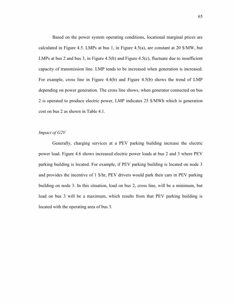
65
Based on the power system operating conditions, locational marginal prices are
calculated in Figure 4.5. LMPs at bus 1, in Figure 4.5(a), are constant at 20 $/MW, but
LMPs at bus 2 and bus 3, in Figure 4.5(b) and Figure 4.5(c), fluctuate due to insufficient
capacity of transmission line. LMP tends to be increased when generation is increased.
For example, cross line in Figure 4.4(b) and Figure 4.5(b) shows the trend of LMP
depending on power generation. The cross line shows, when generator connected on bus
2 is operated to produce electric power, LMP indicates 25 $/MWh which is generation
cost on bus 2 as shown in Table 4.1.
Impact of G2V
Generally, charging services at a PEV parking building increase the electric
power load. Figure 4.6 shows increased electric power loads at bus 2 and 3 where PEV
parking building is located. For example, if PEV parking building is located on node 3
and provides the incentive of 1 $/hr, PEV drivers would park their cars in PEV parking
building on node 3. In this situation, load on bus 2, cross line, will be a minimum, but
load on bus 3 will be a maximum, which results from that PEV parking building is
located with the operating area of bus 3.
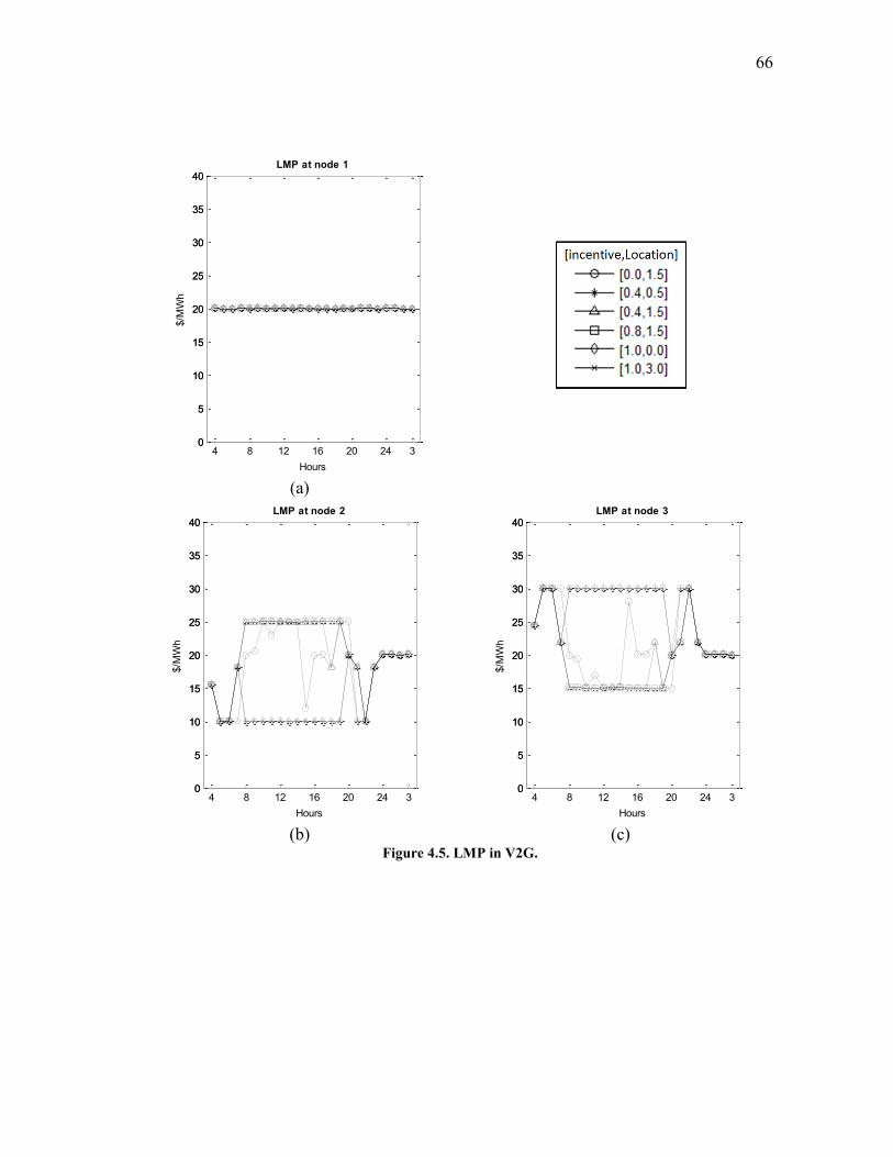
66
(a)
(b) (c)
Figure 4.5. LMP in V2G.
4 8 12 16 20 24 30
5
10
15
20
25
30
35
40
0
5
10
15
20
25
30
35
40LMP at node 1
Hours
$/M
Wh
4 8 12 16 20 24 30
5
10
15
20
25
30
35
40
0
5
10
15
20
25
30
35
40LMP at node 2
Hours$/M
Wh
4 8 12 16 20 24 30
5
10
15
20
25
30
35
40
0
5
10
15
20
25
30
35
40LMP at node 3
Hours
$/M
Wh
4 8 12 16 20 24 30
5
10
15
20
25
30
35
40
0
5
10
15
20
25
30
35
40LMP at node 1
Hours
$/M
Wh
4 8 12 16 20 24 30
5
10
15
20
25
30
35
40
0
5
10
15
20
25
30
35
40LMP at node 2
Hours
$/M
Wh
4 8 12 16 20 24 30
5
10
15
20
25
30
35
40
0
5
10
15
20
25
30
35
40LMP at node 3
Hours
$/M
Wh
4 8 12 16 20 24 30
5
10
15
20
25
30
35
40
0
5
10
15
20
25
30
35
40LMP at node 1
Hours
$/M
Wh
4 8 12 16 20 24 30
5
10
15
20
25
30
35
40
0
5
10
15
20
25
30
35
40LMP at node 2
Hours
$/M
Wh
4 8 12 16 20 24 30
5
10
15
20
25
30
35
40
0
5
10
15
20
25
30
35
40LMP at node 3
Hours
$/M
Wh

67
(a)
(b) (c) Figure 4.6. Power Load in G2V
In G2V mode, Figure 4.7(a) shows increased power generation at bus 1. Electric
power generations at bus 2 and 3 in G2V mode are less than the generation in the V2G
mode because of the absence of power generation from the PEV parking building. In
4 8 12 16 20 24 30
1
2
3
4
5
6
7
8
9
10
0
1
2
3
4
5
6
7
8
9
10Load at node 1
Hours
MW
4 8 12 16 20 24 30
1
2
3
4
5
6
7
8
9
10
0
1
2
3
4
5
6
7
8
9
10Load at node 2
HoursM
W
4 8 12 16 20 24 30
1
2
3
4
5
6
7
8
9
10
0
1
2
3
4
5
6
7
8
9
10Load at node 3
Hours
MW
4 8 12 16 20 24 30
1
2
3
4
5
6
7
8
9
10
0
1
2
3
4
5
6
7
8
9
10Load at node 1
Hours
MW
4 8 12 16 20 24 30
1
2
3
4
5
6
7
8
9
10
0
1
2
3
4
5
6
7
8
9
10Load at node 2
Hours
MW
4 8 12 16 20 24 30
1
2
3
4
5
6
7
8
9
10
0
1
2
3
4
5
6
7
8
9
10Load at node 3
Hours
MW
4 8 12 16 20 24 30
1
2
3
4
5
6
7
8
9
10
0
1
2
3
4
5
6
7
8
9
10Load at node 1
Hours
MW
4 8 12 16 20 24 30
1
2
3
4
5
6
7
8
9
10
0
1
2
3
4
5
6
7
8
9
10Load at node 2
Hours
MW
4 8 12 16 20 24 30
1
2
3
4
5
6
7
8
9
10
0
1
2
3
4
5
6
7
8
9
10Load at node 3
Hours
MW
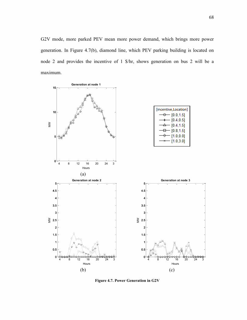
68
G2V mode, more parked PEV mean more power demand, which brings more power
generation. In Figure 4.7(b), diamond line, which PEV parking building is located on
node 2 and provides the incentive of 1 $/hr, shows generation on bus 2 will be a
maximum.
(a)
(b) (c)
Figure 4.7. Power Generation in G2V
4 8 12 16 20 24 30
5
10
15
0
5
10
15Generation at node 1
Hours
MW
4 8 12 16 20 24 30
0.5
1
1.5
2
2.5
3
3.5
4
4.5
5
0
0.5
1
1.5
2
2.5
3
3.5
4
4.5
5Generation at node 2
Hours
MW
4 8 12 16 20 24 30
0.5
1
1.5
2
2.5
3
3.5
4
4.5
5
0
0.5
1
1.5
2
2.5
3
3.5
4
4.5
5Generation at node 3
Hours
MW
4 8 12 16 20 24 30
5
10
15
0
5
10
15Generation at node 1
Hours
MW
4 8 12 16 20 24 30
0.5
1
1.5
2
2.5
3
3.5
4
4.5
5
0
0.5
1
1.5
2
2.5
3
3.5
4
4.5
5Generation at node 2
Hours
MW
4 8 12 16 20 24 30
0.5
1
1.5
2
2.5
3
3.5
4
4.5
5
0
0.5
1
1.5
2
2.5
3
3.5
4
4.5
5Generation at node 3
Hours
MW
4 8 12 16 20 24 30
5
10
15
0
5
10
15Generation at node 1
Hours
MW
4 8 12 16 20 24 30
0.5
1
1.5
2
2.5
3
3.5
4
4.5
5
0
0.5
1
1.5
2
2.5
3
3.5
4
4.5
5Generation at node 2
Hours
MW
4 8 12 16 20 24 30
0.5
1
1.5
2
2.5
3
3.5
4
4.5
5
0
0.5
1
1.5
2
2.5
3
3.5
4
4.5
5Generation at node 3
Hours
MW
69
Figure 4.8 shows LMP in G2V. Like LMP in V2G mode, LMP in G2V mode
also tends to be increased when generation is increased. While LMP at bus 1 where
electricity is produced in the lowest price, shows a constant value of 20 $/MWh, LMP at
bus 2 and bus 3 is fluctuated due to changing power system operating condition.
(a)
(b) (c)
Figure 4.8. LMP in G2V
4 8 12 16 20 24 30
5
10
15
20
25
30
35
40
0
5
10
15
20
25
30
35
40LMP at node 1
Hours
$/M
Wh
4 8 12 16 20 24 30
5
10
15
20
25
30
35
40
0
5
10
15
20
25
30
35
40LMP at node 2
Hours
$/M
Wh
4 8 12 16 20 24 30
5
10
15
20
25
30
35
40
0
5
10
15
20
25
30
35
40LMP at node 3
Hours
$/M
Wh
4 8 12 16 20 24 30
5
10
15
20
25
30
35
40
0
5
10
15
20
25
30
35
40LMP at node 1
Hours
$/M
Wh
4 8 12 16 20 24 30
5
10
15
20
25
30
35
40
0
5
10
15
20
25
30
35
40LMP at node 2
Hours
$/M
Wh
4 8 12 16 20 24 30
5
10
15
20
25
30
35
40
0
5
10
15
20
25
30
35
40LMP at node 3
Hours
$/M
Wh
4 8 12 16 20 24 30
5
10
15
20
25
30
35
40
0
5
10
15
20
25
30
35
40LMP at node 1
Hours
$/M
Wh
4 8 12 16 20 24 30
5
10
15
20
25
30
35
40
0
5
10
15
20
25
30
35
40LMP at node 2
Hours
$/M
Wh
4 8 12 16 20 24 30
5
10
15
20
25
30
35
40
0
5
10
15
20
25
30
35
40LMP at node 3
Hours
$/M
Wh
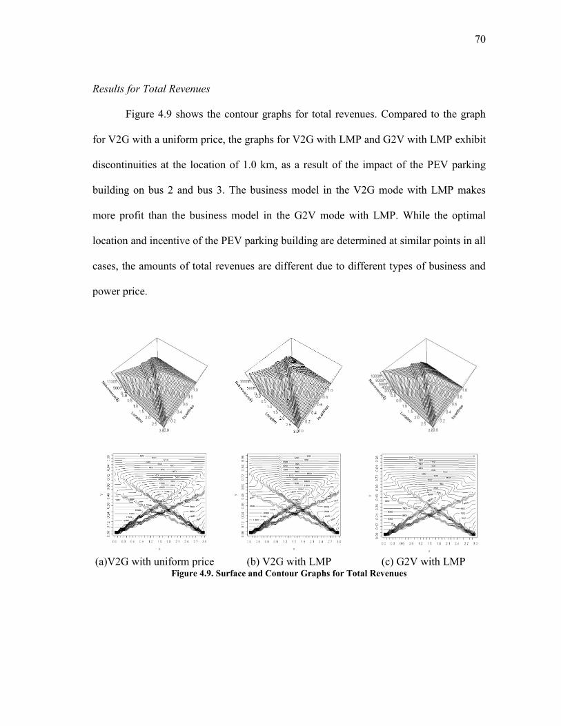
70
Results for Total Revenues
Figure 4.9 shows the contour graphs for total revenues. Compared to the graph
for V2G with a uniform price, the graphs for V2G with LMP and G2V with LMP exhibit
discontinuities at the location of 1.0 km, as a result of the impact of the PEV parking
building on bus 2 and bus 3. The business model in the V2G mode with LMP makes
more profit than the business model in the G2V mode with LMP. While the optimal
location and incentive of the PEV parking building are determined at similar points in all
cases, the amounts of total revenues are different due to different types of business and
power price.
(a)V2G with uniform price (b) V2G with LMP (c) G2V with LMP
Figure 4.9. Surface and Contour Graphs for Total Revenues
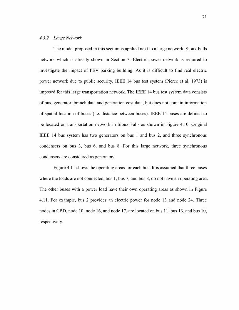
71
4.3.2 Large Network
The model proposed in this section is applied next to a large network, Sioux Falls
network which is already shown in Section 3. Electric power network is required to
investigate the impact of PEV parking building. As it is difficult to find real electric
power network due to public security, IEEE 14 bus test system (Pierce et al. 1973) is
imposed for this large transportation network. The IEEE 14 bus test system data consists
of bus, generator, branch data and generation cost data, but does not contain information
of spatial location of buses (i.e. distance between buses). IEEE 14 buses are defined to
be located on transportation network in Sioux Falls as shown in Figure 4.10. Original
IEEE 14 bus system has two generators on bus 1 and bus 2, and three synchronous
condensers on bus 3, bus 6, and bus 8. For this large network, three synchronous
condensers are considered as generators.
Figure 4.11 shows the operating areas for each bus. It is assumed that three buses
where the loads are not connected, bus 1, bus 7, and bus 8, do not have an operating area.
The other buses with a power load have their own operating areas as shown in Figure
4.11. For example, bus 2 provides an electric power for node 13 and node 24. Three
nodes in CBD, node 10, node 16, and node 17, are located on bus 11, bus 13, and bus 10,
respectively.
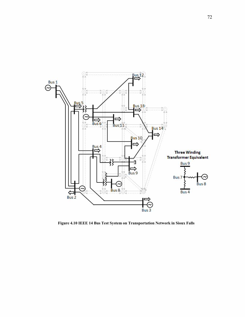
72
Figure 4.10 IEEE 14 Bus Test System on Transportation Network in Sioux Falls
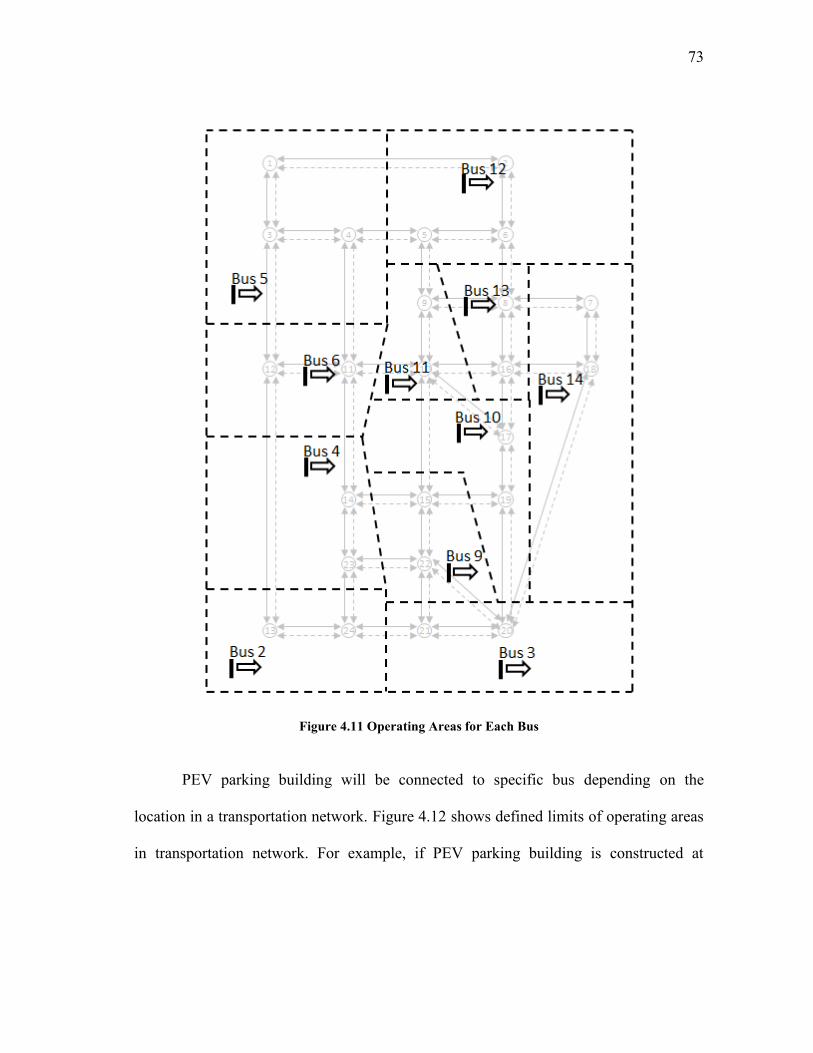
73
Figure 4.11 Operating Areas for Each Bus
PEV parking building will be connected to specific bus depending on the
location in a transportation network. Figure 4.12 shows defined limits of operating areas
in transportation network. For example, if PEV parking building is constructed at

74
distance 0.8 from node 10 on the link between node 10 and node 16, PEV parking
building would be connected to bus 13.
Figure 4.12 Limits of Operating Areas in Transportation Network
Generator data of IEEE 14 bus test system is modified for three additional
generators. Table 4.2 shows detail values of modified generator data. Basically, the
modified generator data is referred from IEEE 14 bus test system, but values in bold
fonts are assumed for this large network. Notation for first row in Table 4.2 can be
found in APPENDIX V.
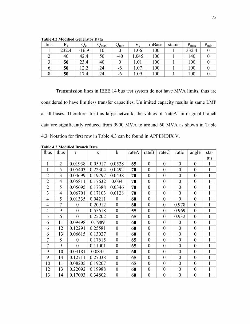
75
Table 4.2 Modified Generator Data
bus Pg Qg Qmax Qmin Vg mBase status Pmax Pmin
1 232.4 -16.9 10 0 1.06 100 1 332.4 0
2 40 42.4 50 -40 1.045 100 1 140 0
3 50 23.4 40 0 1.01 100 1 100 0
6 50 12.2 24 -6 1.07 100 1 100 0
8 50 17.4 24 -6 1.09 100 1 100 0
Transmission lines in IEEE 14 bus test system do not have MVA limits, thus are
considered to have limitless transfer capacities. Unlimited capacity results in same LMP
at all buses. Therefore, for this large network, the values of ‘rateA’ in original branch
data are significantly reduced from 9900 MVA to around 60 MVA as shown in Table
4.3. Notation for first row in Table 4.3 can be found in APPENDIX V.
Table 4.3 Modified Branch Data
fbus tbus r x b rateA rateB rateC ratio angle sta-
tus
1 2 0.01938 0.05917 0.0528 65 0 0 0 0 1
1 5 0.05403 0.22304 0.0492 70 0 0 0 0 1
2 3 0.04699 0.19797 0.0438 70 0 0 0 0 1
2 4 0.05811 0.17632 0.034 70 0 0 0 0 1
2 5 0.05695 0.17388 0.0346 70 0 0 0 0 1
3 4 0.06701 0.17103 0.0128 70 0 0 0 0 1
4 5 0.01335 0.04211 0 60 0 0 0 0 1
4 7 0 0.20912 0 60 0 0 0.978 0 1
4 9 0 0.55618 0 55 0 0 0.969 0 1
5 6 0 0.25202 0 65 0 0 0.932 0 1
6 11 0.09498 0.1989 0 60 0 0 0 0 1
6 12 0.12291 0.25581 0 60 0 0 0 0 1
6 13 0.06615 0.13027 0 60 0 0 0 0 1
7 8 0 0.17615 0 65 0 0 0 0 1
7 9 0 0.11001 0 65 0 0 0 0 1
9 10 0.03181 0.0845 0 60 0 0 0 0 1
9 14 0.12711 0.27038 0 65 0 0 0 0 1
10 11 0.08205 0.19207 0 65 0 0 0 0 1
12 13 0.22092 0.19988 0 60 0 0 0 0 1
13 14 0.17093 0.34802 0 60 0 0 0 0 1

76
For this large network, power generation cost at bus i is defined as polynomial
model as Equation 4.9.
Coefficients for each generation bus are referred from generator cost data of
IEEE 14 bus test system. Coefficients for generation bus 3, bus 6, and bus 8 are same,
thus the values in bus 3 and bus 6 are modified to consider generation in different
generation costs. The modified generator cost data is as shown in Table 4.4.
Table 4.4 Modified Generator Cost Data
Generation
Bus no. 2ic
1ic
0ic
1 0.043 20 0
2 0.250 20 0
3 0.100 30 0
6 0.050 35 0
8 0.010 40 0
The sections first shows the result of the optimal incentive structure, location of
PEV parking building, and the total revenues in V2G operation with LMP and in G2V
operation with LMP. Next, based on the optimal decisions, the impact of V2G and G2V
operations on electric power system is presented in the form of generation, load, and
LMP on each bus.
Results—Total Revenues
Based on the modified IEEE 14 bus test data, PEV parking building model finds
the optimal location and incentive structure with V2G and G2V operations. Figure 4.13
2 1 0
2
i gi i gi i gi iC P c P c P c (4.9)
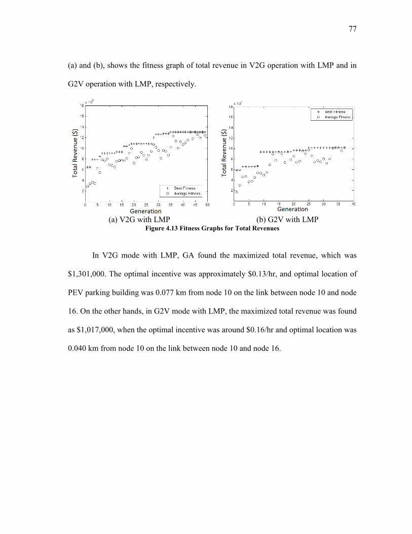
77
(a) and (b), shows the fitness graph of total revenue in V2G operation with LMP and in
G2V operation with LMP, respectively.
(a) V2G with LMP (b) G2V with LMP
Figure 4.13 Fitness Graphs for Total Revenues
In V2G mode with LMP, GA found the maximized total revenue, which was
$1,301,000. The optimal incentive was approximately $0.13/hr, and optimal location of
PEV parking building was 0.077 km from node 10 on the link between node 10 and node
16. On the other hands, in G2V mode with LMP, the maximized total revenue was found
as $1,017,000, when the optimal incentive was around $0.16/hr and optimal location was
0.040 km from node 10 on the link between node 10 and node 16.
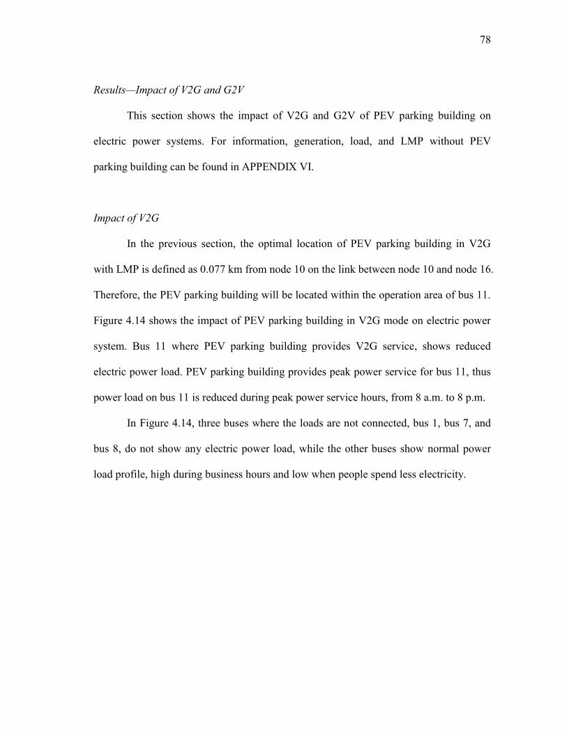
78
Results—Impact of V2G and G2V
This section shows the impact of V2G and G2V of PEV parking building on
electric power systems. For information, generation, load, and LMP without PEV
parking building can be found in APPENDIX VI.
Impact of V2G
In the previous section, the optimal location of PEV parking building in V2G
with LMP is defined as 0.077 km from node 10 on the link between node 10 and node 16.
Therefore, the PEV parking building will be located within the operation area of bus 11.
Figure 4.14 shows the impact of PEV parking building in V2G mode on electric power
system. Bus 11 where PEV parking building provides V2G service, shows reduced
electric power load. PEV parking building provides peak power service for bus 11, thus
power load on bus 11 is reduced during peak power service hours, from 8 a.m. to 8 p.m.
In Figure 4.14, three buses where the loads are not connected, bus 1, bus 7, and
bus 8, do not show any electric power load, while the other buses show normal power
load profile, high during business hours and low when people spend less electricity.

79
Figure 4.14 Power Load in V2G of Large Network
Figure 4.15 shows generation on each generation bus. Bus 1 with cheapest initial
generation cost generates the most amount of electricity, while bus 5 with most
expensive initial generation cost does not generate any amount of electricity. Bus 3 and
bus 4 generate electricity during specific hours when power demand is high.

80
Figure 4.15 Power Generation in V2G of Large Network
Figure 4.16 shows LMP for one day on each bus. Bus 1 where power generator
with the cheapest initial generation cost is installed, presents the lowest LMP. On the
other hands, the other bus shows similar LMP patterns, high LMP during business hours
and low LMP during a night.

81
Figure 4.16 LMP in V2G of Large Network
Impact of G2V
In the previous section, the optimal location of PEV parking building in G2V
with LMP is defined as 0.040 km from node 10 on the link between node 10 and node 16.
Therefore, the PEV parking building will be located within the operation area of bus 11.
Figure 4.17 shows electric power load on bus 11 is increased by amount of electricity for
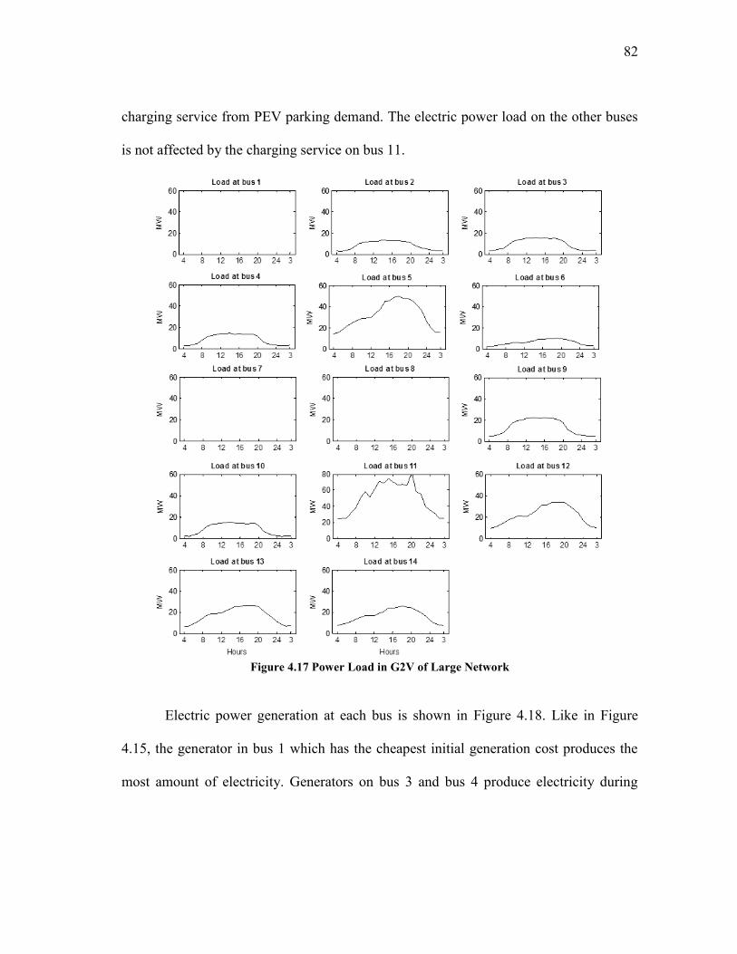
82
charging service from PEV parking demand. The electric power load on the other buses
is not affected by the charging service on bus 11.
Figure 4.17 Power Load in G2V of Large Network
Electric power generation at each bus is shown in Figure 4.18. Like in Figure
4.15, the generator in bus 1 which has the cheapest initial generation cost produces the
most amount of electricity. Generators on bus 3 and bus 4 produce electricity during

83
business hours, from 8 a.m. to 8 p.m. Especially, generator on bus 5 which have the most
expensive initial generation cost is operated for peak hour demand.
Figure 4.18 Power Generation in G2V of Large Network
LMP has a similar pattern, high during business hours and low during a night,
and LMP at bus 1 is the lowest among LMPs on all buses. Comparing to LMP in V2G,
LMP in G2V shows a little higher price, which results from the additional electric power
demand from G2V service of PEV parking building.
From the results for impact of V2G and G2V, it is confirmed that PEV parking
building has an effect on generation, load, and LMP. Figure 4.14 and Figure 4.17 shows
electricity, extracted from PEVs or used to charge PEVs, directly affects electricity
power load on the bus where PEV parking building is located. On the other hands, power
generation and LMP are influenced by the load changed by V2G and G2V operations.
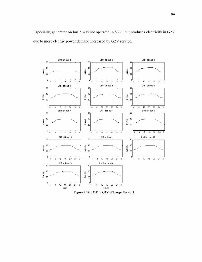
84
Especially, generator on bus 5 was not operated in V2G, but produces electricity in G2V
due to more electric power demand increased by G2V service.
Figure 4.19 LMP in G2V of Large Network

85
4.4 Summary
This section presented a model to account for the impact of a PEV parking
building on a power system and the total revenue of a developer. A PEV parking
building represents an interface station point between a transportation network and an
electric power network. Hence, a developer’s decision on location and incentive affects
the traffic flow on the transportation network and the electric power flow on the electric
power network.
In this section, optimal traffic flow was evaluated by the user equilibrium
problem, which reveals PEV parking demand. Also, optimal power flow was evaluated
by the optimal power flow problem. The results of the numerical example in this section
verify the impact of a PEV parking building on power system operating conditions and
locational marginal prices. The optimal location and incentive of a PEV parking building
was evaluated using the total revenue model. The results of total revenue show that the
business model of V2G with LMP results in the most benefit for a developer.
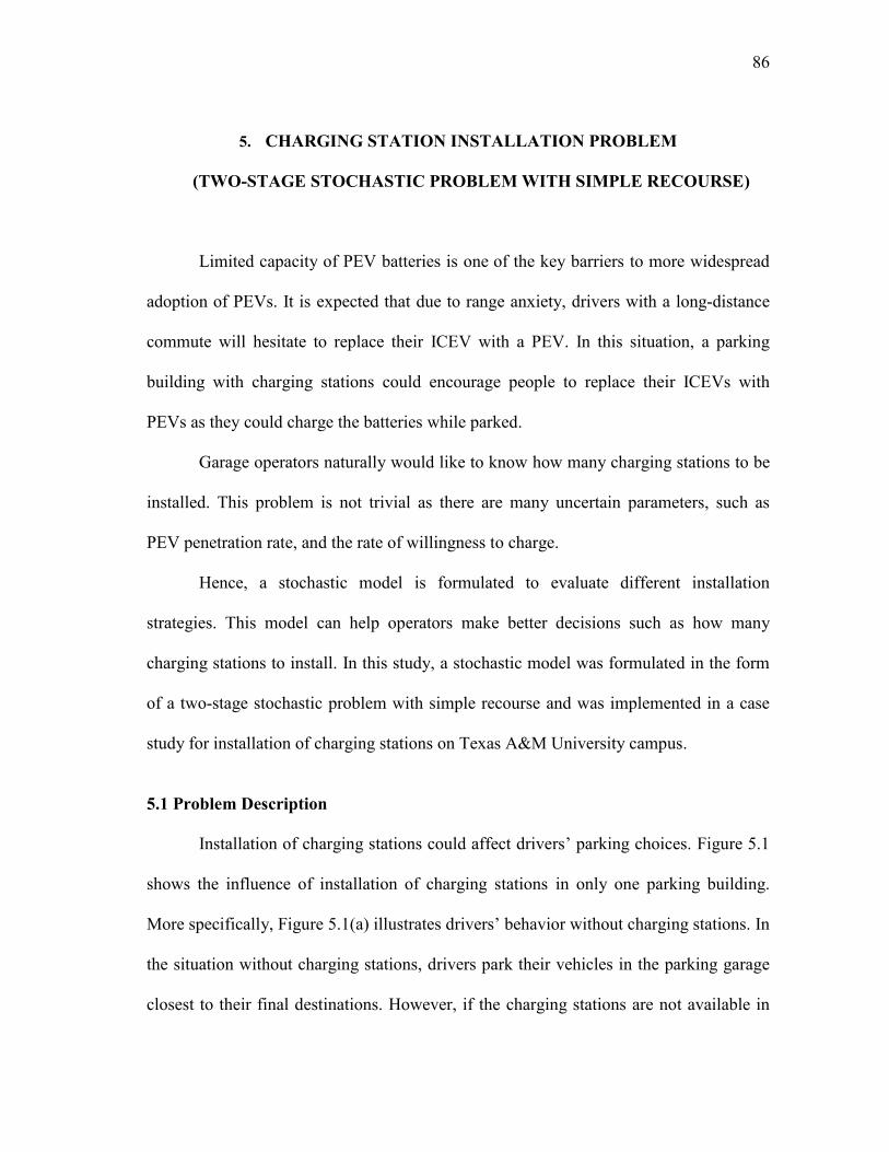
86
5. CHARGING STATION INSTALLATION PROBLEM
(TWO-STAGE STOCHASTIC PROBLEM WITH SIMPLE RECOURSE)
Limited capacity of PEV batteries is one of the key barriers to more widespread
adoption of PEVs. It is expected that due to range anxiety, drivers with a long-distance
commute will hesitate to replace their ICEV with a PEV. In this situation, a parking
building with charging stations could encourage people to replace their ICEVs with
PEVs as they could charge the batteries while parked.
Garage operators naturally would like to know how many charging stations to be
installed. This problem is not trivial as there are many uncertain parameters, such as
PEV penetration rate, and the rate of willingness to charge.
Hence, a stochastic model is formulated to evaluate different installation
strategies. This model can help operators make better decisions such as how many
charging stations to install. In this study, a stochastic model was formulated in the form
of a two-stage stochastic problem with simple recourse and was implemented in a case
study for installation of charging stations on Texas A&M University campus.
5.1 Problem Description
Installation of charging stations could affect drivers’ parking choices. Figure 5.1
shows the influence of installation of charging stations in only one parking building.
More specifically, Figure 5.1(a) illustrates drivers’ behavior without charging stations. In
the situation without charging stations, drivers park their vehicles in the parking garage
closest to their final destinations. However, if the charging stations are not available in
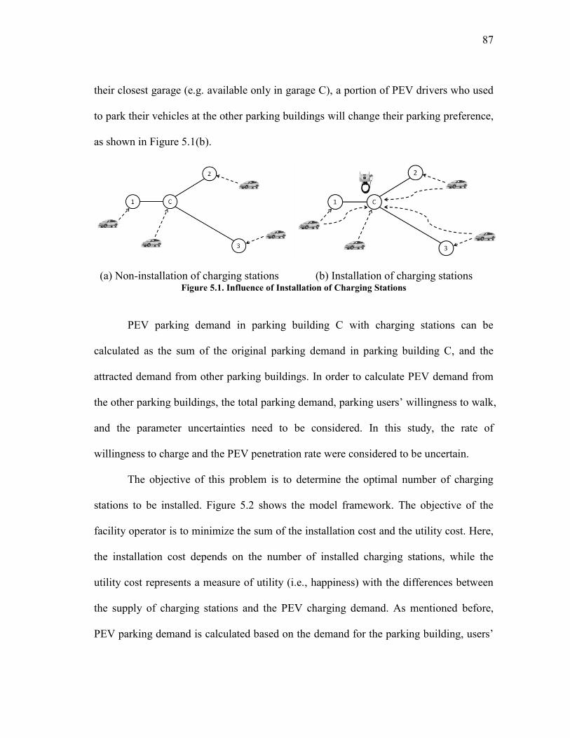
87
their closest garage (e.g. available only in garage C), a portion of PEV drivers who used
to park their vehicles at the other parking buildings will change their parking preference,
as shown in Figure 5.1(b).
(a) Non-installation of charging stations (b) Installation of charging stations Figure 5.1. Influence of Installation of Charging Stations
PEV parking demand in parking building C with charging stations can be
calculated as the sum of the original parking demand in parking building C, and the
attracted demand from other parking buildings. In order to calculate PEV demand from
the other parking buildings, the total parking demand, parking users’ willingness to walk,
and the parameter uncertainties need to be considered. In this study, the rate of
willingness to charge and the PEV penetration rate were considered to be uncertain.
The objective of this problem is to determine the optimal number of charging
stations to be installed. Figure 5.2 shows the model framework. The objective of the
facility operator is to minimize the sum of the installation cost and the utility cost. Here,
the installation cost depends on the number of installed charging stations, while the
utility cost represents a measure of utility (i.e., happiness) with the differences between
the supply of charging stations and the PEV charging demand. As mentioned before,
PEV parking demand is calculated based on the demand for the parking building, users’
88
willingness to walk, and the two PEV uncertain parameters, namely PEV penetration
rate and the rate of willingness to charge.
Figure 5.2. Model Framework
5.2 The Model
The model developed in this section is a two-stage stochastic problem with
simple recourse; the first stage allocates the spaces for the charging stations, and the
second stage assesses operator’s utility. The objective of this problem is to minimize the
sum of the installation cost and the utility cost, as shown in Equation 5.1. The constraints

89
associated with the first stage are the space capacity for charging stations in Equation 5.2.
The notations of parameters, variables, and sets used in the model are as follows:
Sets
pN = the set of parking nodes
Parameters
N = the maximum number of charging stations to be installed
s
in hq = the trip rate to node s on time h
s
out hq = the trip rate from node s on time h
Variables
d = average PEV demand of parking garage
hd = PEV demand of parking garage on time h
f
= the installation cost
sl
= the minimum distance from node s to the parking garage
n
= the number of charging stations
jQ
= the developer’s utility cost
W
= the attraction rate by walking distance
c hx
= the sum of trip rates of PEVs entering the parking garage
d hx
= the sum of trip rates of PEVs exiting the parking garage
Random Variables
1 = PEV penetration rate
2 = PEV charging rate
1
= realization of 1
2
= realization of 2
1P = 1 1P
2P = 2 2P
90
The charging station installation (CSI) problem is formulated as follows:
min f n E Q d n (5.1)
s.t. 0 and integern N (5.2)
1 2
1 1 2 2
where E Q d n P P Q d n
(5.3)
24
1
1
24h
h
d d
(5.4)
1 1 1c dd x x
(5.5)
1 2, ,24h h c dh hd d x x h
(5.6)
1 2 1, ,24p
s s
c inh hs N
x q W l h
(5.7)
1 2 1, ,24p
s s
d outh hs N
x q W l h
(5.8)
jQ d n represents the utility cost if n charging stations were installed when
actual PEV parking demand was d . The motivation for this formulation is to account
for the opportunity cost. The PEV parking demand is defined as the average of hourly
PEV demands during one day, as shown in Equation 5.4.
Random variables of 1 and 2 represent uncertainty in parameters. 1
represents the future PEV penetration rate, and 2 represents the rate of willingness to
charge. The sum of the PEV trip rates entering and exiting the parking garage, c hx and
d hx , are derived from the original trip rates, random variables, and attraction rate
function. This model is also referred to as the charging station installation problem.
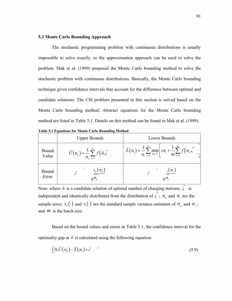
91
5.3 Monte Carlo Bounding Approach
The stochastic programming problem with continuous distributions is usually
impossible to solve exactly, so the approximation approach can be used to solve the
problem. Mak et al. (1999) proposed the Monte Carlo bounding method to solve the
stochastic problem with continuous distributions. Basically, the Monte Carlo bounding
technique gives confidence intervals that account for the difference between optimal and
candidate solutions. The CSI problem presented in this section is solved based on the
Monte Carlo bounding method. Abstract equations for the Monte Carlo bounding
method are listed in Table 5.1. Details on this method can be found in Mak et al. (1999).
Table 5.1 Equations for Monte Carlo Bounding Method
Upper Bounds Lower Bounds
Bound
Value
1
1ˆ,
uni
u
iu
U n f nn
1 1
1 1min ,
l
i
n mij
l i in X
i jl
L n cn f nn m
Bound
Error
1,un u u
u
u
t s n
n
1,ln l l
l
l
t s n
n
Note: where n̂ is a candidate solution of optimal number of charging stations; i is
independent and identically distributed from the distribution of ; un and ln are the
sample sizes; us and ls are the standard sample variance estimator of u and l ;
and m is the batch size.
Based on the bound values and errors in Table 5.1, the confidence interval for the
optimality gap at n̂ is calculated using the following equation:
0, u l u lU n L n (5.9)

92
5.4 Case Study
In order to demonstrate the CSI problem, the CSI project of Texas A&M
University was considered for the case study. For this case study, data of parking entry
and exit, parking capacity of parking buildings and lots, and location of parking
buildings and lots were collected and measured. Data that were difficult to measure were
assumed to be as realistic as possible.
5.4.1 Area Scope
There are a number of parking buildings and open parking lots on the Texas
A&M University campus in College Station, Texas. This case study considered only five
parking garages and six surface parking lots, as shown in Figure 5.3.
The capacity of parking spaces for each parking garage and open space lot is
shown in Table 5.2.
Table 5.2 Parking Spaces
Parking ID Spaces Parking ID Spaces
S1 775 G1 2,000
S2 2,300 G2 510
S3 370 G3 3,100
S4 640 G4 1,630
S5 2,350 G5 2,250
S6 1,180
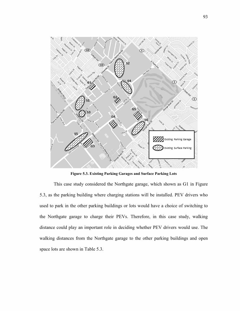
93
Figure 5.3. Existing Parking Garages and Surface Parking Lots
This case study considered the Northgate garage, which shown as G1 in Figure
5.3, as the parking building where charging stations will be installed. PEV drivers who
used to park in the other parking buildings or lots would have a choice of switching to
the Northgate garage to charge their PEVs. Therefore, in this case study, walking
distance could play an important role in deciding whether PEV drivers would use. The
walking distances from the Northgate garage to the other parking buildings and open
space lots are shown in Table 5.3.
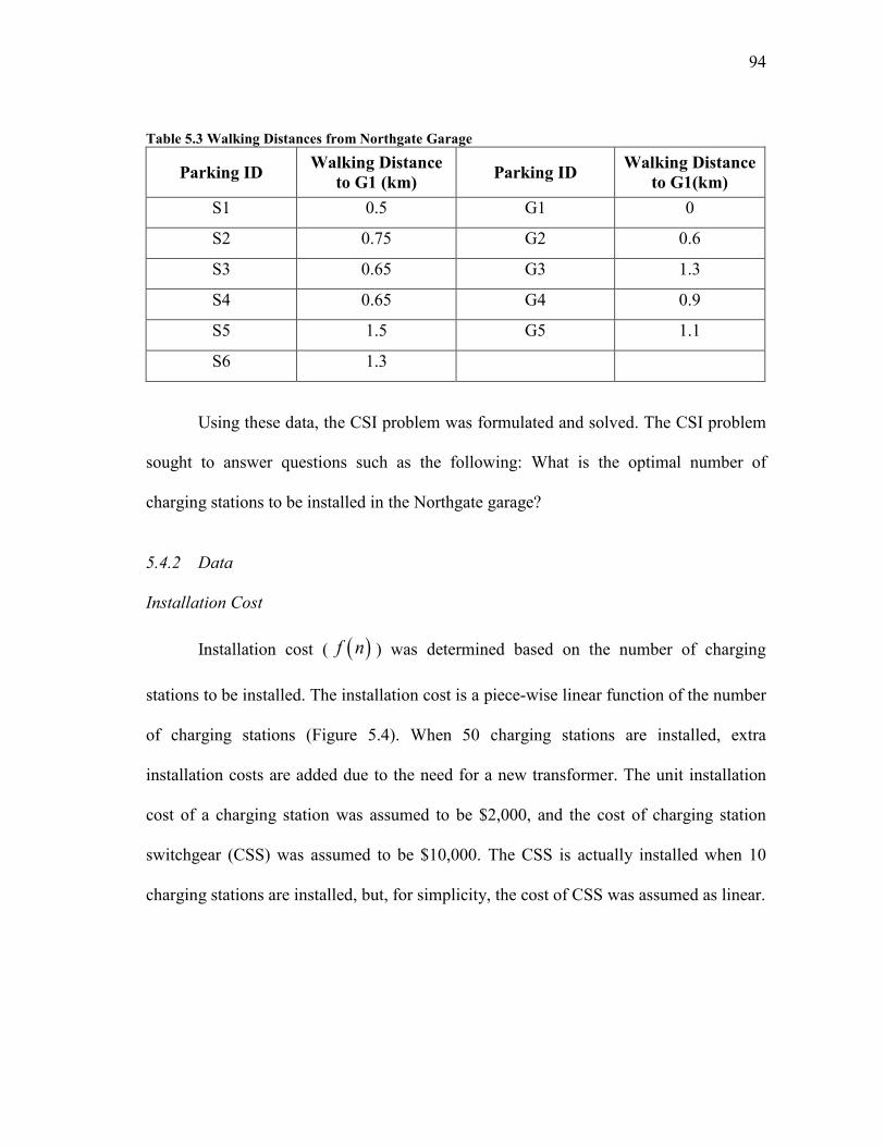
94
Table 5.3 Walking Distances from Northgate Garage
Parking ID Walking Distance
to G1 (km) Parking ID
Walking Distance
to G1(km)
S1 0.5 G1 0
S2 0.75 G2 0.6
S3 0.65 G3 1.3
S4 0.65 G4 0.9
S5 1.5 G5 1.1
S6 1.3
Using these data, the CSI problem was formulated and solved. The CSI problem
sought to answer questions such as the following: What is the optimal number of
charging stations to be installed in the Northgate garage?
5.4.2 Data
Installation Cost
Installation cost ( f n ) was determined based on the number of charging
stations to be installed. The installation cost is a piece-wise linear function of the number
of charging stations (Figure 5.4). When 50 charging stations are installed, extra
installation costs are added due to the need for a new transformer. The unit installation
cost of a charging station was assumed to be $2,000, and the cost of charging station
switchgear (CSS) was assumed to be $10,000. The CSS is actually installed when 10
charging stations are installed, but, for simplicity, the cost of CSS was assumed as linear.
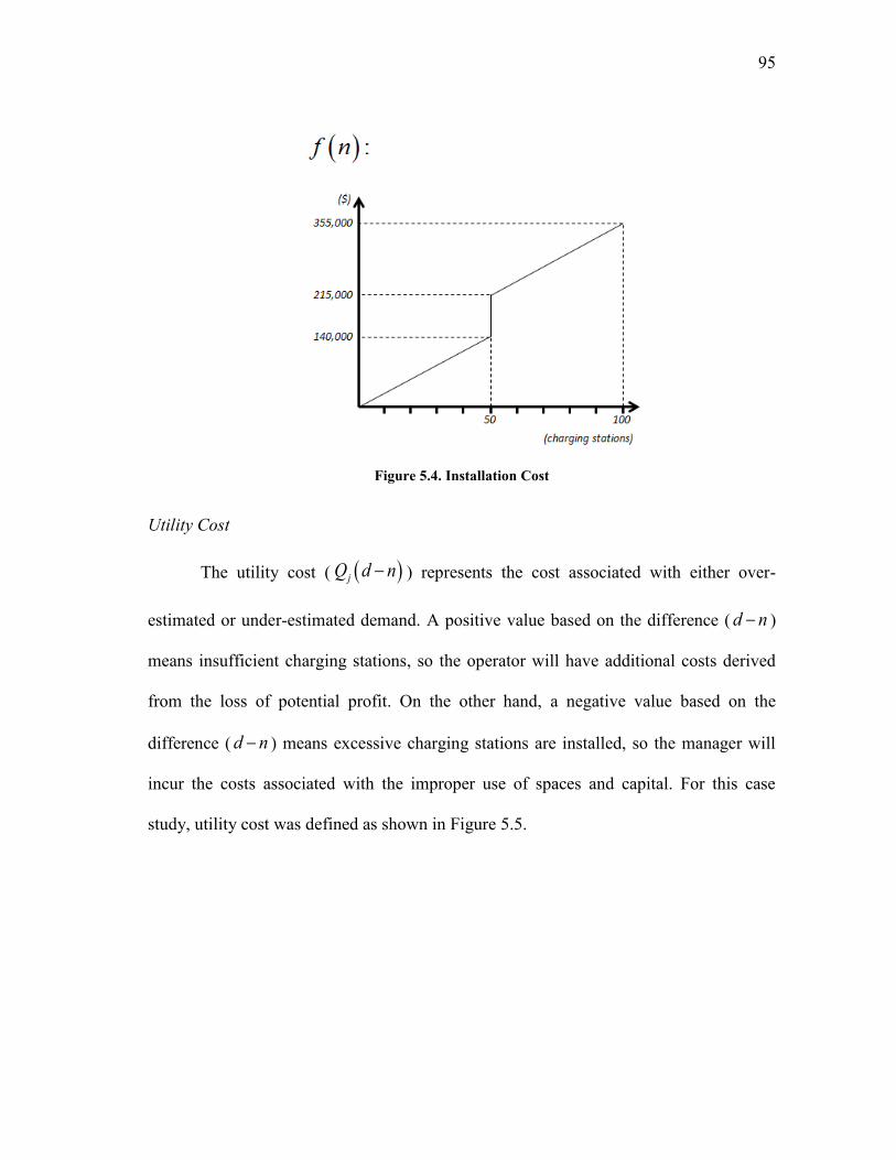
95
Figure 5.4. Installation Cost
Utility Cost
The utility cost ( jQ d n ) represents the cost associated with either over-
estimated or under-estimated demand. A positive value based on the difference ( d n )
means insufficient charging stations, so the operator will have additional costs derived
from the loss of potential profit. On the other hand, a negative value based on the
difference ( d n ) means excessive charging stations are installed, so the manager will
incur the costs associated with the improper use of spaces and capital. For this case
study, utility cost was defined as shown in Figure 5.5.
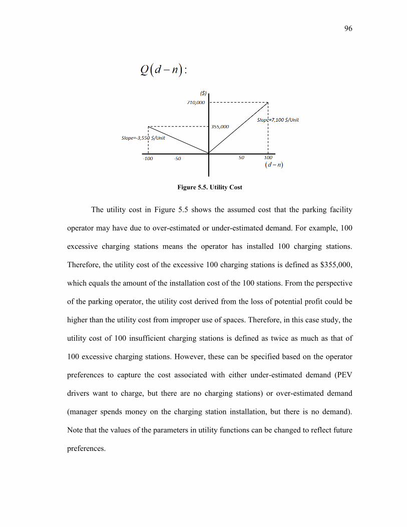
96
Figure 5.5. Utility Cost
The utility cost in Figure 5.5 shows the assumed cost that the parking facility
operator may have due to over-estimated or under-estimated demand. For example, 100
excessive charging stations means the operator has installed 100 charging stations.
Therefore, the utility cost of the excessive 100 charging stations is defined as $355,000,
which equals the amount of the installation cost of the 100 stations. From the perspective
of the parking operator, the utility cost derived from the loss of potential profit could be
higher than the utility cost from improper use of spaces. Therefore, in this case study, the
utility cost of 100 insufficient charging stations is defined as twice as much as that of
100 excessive charging stations. However, these can be specified based on the operator
preferences to capture the cost associated with either under-estimated demand (PEV
drivers want to charge, but there are no charging stations) or over-estimated demand
(manager spends money on the charging station installation, but there is no demand).
Note that the values of the parameters in utility functions can be changed to reflect future
preferences.
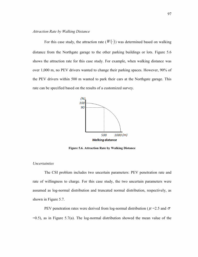
97
Attraction Rate by Walking Distance
For this case study, the attraction rate ( W ) was determined based on walking
distance from the Northgate garage to the other parking buildings or lots. Figure 5.6
shows the attraction rate for this case study. For example, when walking distance was
over 1,000 m, no PEV drivers wanted to change their parking spaces. However, 90% of
the PEV drivers within 500 m wanted to park their cars at the Northgate garage. This
rate can be specified based on the results of a customized survey.
Figure 5.6. Attraction Rate by Walking Distance
Uncertainties
The CSI problem includes two uncertain parameters: PEV penetration rate and
rate of willingness to charge. For this case study, the two uncertain parameters were
assumed as log-normal distribution and truncated normal distribution, respectively, as
shown in Figure 5.7.
PEV penetration rates were derived from log-normal distribution ( =2.5 and
=0.5), as in Figure 5.7(a). The log-normal distribution showed the mean value of the
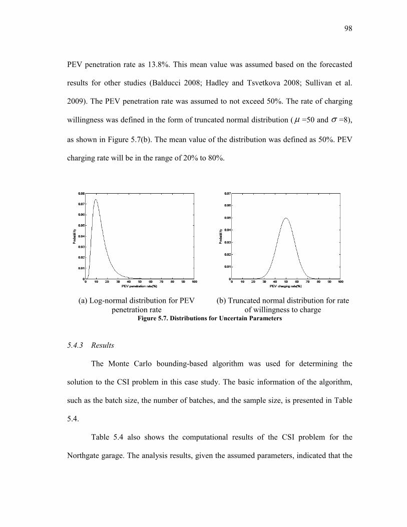
98
PEV penetration rate as 13.8%. This mean value was assumed based on the forecasted
results for other studies (Balducci 2008; Hadley and Tsvetkova 2008; Sullivan et al.
2009). The PEV penetration rate was assumed to not exceed 50%. The rate of charging
willingness was defined in the form of truncated normal distribution ( =50 and =8),
as shown in Figure 5.7(b). The mean value of the distribution was defined as 50%. PEV
charging rate will be in the range of 20% to 80%.
(a) Log-normal distribution for PEV
penetration rate
(b) Truncated normal distribution for rate
of willingness to charge Figure 5.7. Distributions for Uncertain Parameters
5.4.3 Results
The Monte Carlo bounding-based algorithm was used for determining the
solution to the CSI problem in this case study. The basic information of the algorithm,
such as the batch size, the number of batches, and the sample size, is presented in Table
5.4.
Table 5.4 also shows the computational results of the CSI problem for the
Northgate garage. The analysis results, given the assumed parameters, indicated that the
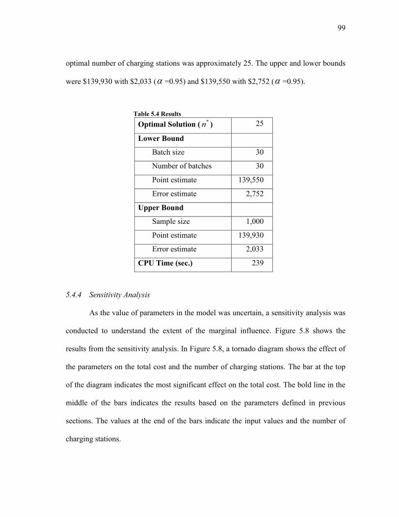
99
optimal number of charging stations was approximately 25. The upper and lower bounds
were $139,930 with $2,033 ( =0.95) and $139,550 with $2,752 ( =0.95).
Table 5.4 Results
Optimal Solution (*n ) 25
Lower Bound
Batch size 30
Number of batches 30
Point estimate 139,550
Error estimate 2,752
Upper Bound
Sample size 1,000
Point estimate 139,930
Error estimate 2,033
CPU Time (sec.) 239
5.4.4 Sensitivity Analysis
As the value of parameters in the model was uncertain, a sensitivity analysis was
conducted to understand the extent of the marginal influence. Figure 5.8 shows the
results from the sensitivity analysis. In Figure 5.8, a tornado diagram shows the effect of
the parameters on the total cost and the number of charging stations. The bar at the top
of the diagram indicates the most significant effect on the total cost. The bold line in the
middle of the bars indicates the results based on the parameters defined in previous
sections. The values at the end of the bars indicate the input values and the number of
charging stations.

100
Figure 5.8. Results of Sensitivity Analysis
For example, the value for the mean of the PEV penetration rate was initially
assumed to be 13.8%. For the sensitivity analysis, the PEV penetration rate was
modified to 12.4% and 15.2% as the values at the end of a bar. The result using the
12.4% PEV penetration rate showed a decrease in the total cost to around $127,000, and
the optimal number of charging stations decreased to 23. On the other hand, the result
using 15.2% showed an increase in the total cost to around $155,000, and the optimal
number of charging stations increased to 28.
Additional findings from the study are as follows:
The mean of the PEV penetration rate and rate of willingness to charge showed
the most significant effect on total cost and the number of charging stations,
respectively.
The utility cost and the mean of the rate of willingness to charge showed a
significant effect on both total cost and the number of charging stations.
101
The unit installation cost showed a moderate effect on both the total cost and
the number of charging stations.
Standard deviation (SD) of the PEV penetration rate showed a moderate effect
on total cost but no effect on the number of charging stations.
The SD of the rate of willingness to charge showed a slight effect on both total
cost and the number of charging stations.
Some managerial implications can be suggested based on the results of the
sensitivity analysis. First, the parking facility operator should focus more on forecasting
the mean values of the two random variables (PEV penetration rate and rate of
willingness to charge) at the planning stage. These are critical values in determining the
total cost and the number of charging stations. Second, in order to reduce the total cost, it
is recommended that managers reduce the utility cost and unit installation cost. Unlike
the uncertain rates, these two costs may be manipulated by the parking operator based on
policies to encourage the use of PEVs.
5.5 Summary
This section presented a model to determine the optimal number of charging
stations to be installed in a single parking building, which was applied to the Northgate
garage project on the Texas A&M University campus in College Station. The model
calculated the PEV parking demand at the Northgate garage and considered uncertainty
in parameters, such as the PEV penetration rate and rate of willingness to charge, as well
as the attraction rate. The Monte Carlo bounding-based algorithm was used to solve this

102
CSI problem. The analysis result showed the optimal number of charging stations and
the upper and the lower bounds of the total cost. Sensitivity analysis suggested that the
facility manager should be careful in determining utility cost.
103
6. CHARGING STATION INSTALLATION PROBLEM
WITH DECISION-DEPENDENT ASSESSMENT OF UNCERTAINTY
(TWO-STAGE STOCHASTIC PROBLEM WITH RECOURSE)
The CSI problem in Section 5 identified the number of charging stations that
minimizes the total cost. The CSI problem had only one decision variable: the number of
charging stations to be installed in the first stage. In addition, the CSI problem in Section
5 did not consider that the decision in the first stage has an effect on realization of
uncertain parameters.
This section presents a charging station installation problem with decision-
dependent assessment of uncertainty (CSI-DDAU problem). The problem has two
decision variables—decisions at first and second stages—and includes the impact of the
first decision on uncertainties. The next section will present an overview of the problem
and model framework. Section 6.2 presents the charging station installation problem
with decision-dependent assessment of uncertainty. In Section 6.3, the decision-
dependent assessment of uncertainty is explained in detail. The case study for the CSI-
DDAU problem is provided in Section 6.4.
6.1 Problem Description
The influence of the installing charging stations at specific garage location on
parking choices, described in the previous section, is considered in this section as well.
That is, the installation of charging stations can change PEV drivers’ parking choices.
104
The difference between the CSI-DDAU problem (in the form of full recourse stochastic
programming) and the CSI problem (in the form of simple recourse stochastic
programming) from the previous section is that the parking operator makes two
decisions in the CSI-DDAU problem. The first decision is made in the first stage with
primary uncertainties, the second decision is made in the second stage with updated
uncertainties. After making the first decision, operators have time to observe the change
in the PEV penetration rate and rate of willingness to charge, and they make a second
stage decision with more information about uncertain parameters.
The objective of this problem is to determine the optimal number of charging
stations, like in the CSI problem. Figure 6.1 shows the model framework. Compared to
the model framework for the CSI problem, the CSI-DDAU problem uses a Bayesian
updating process. While the first decision, the number of initially installed charging
stations affects installation cost 1, utility cost, and Bayesian updating of the distribution
of uncertain parameters, the second decision, the number of additional charging stations,
affects only installation cost 2 and utility cost.
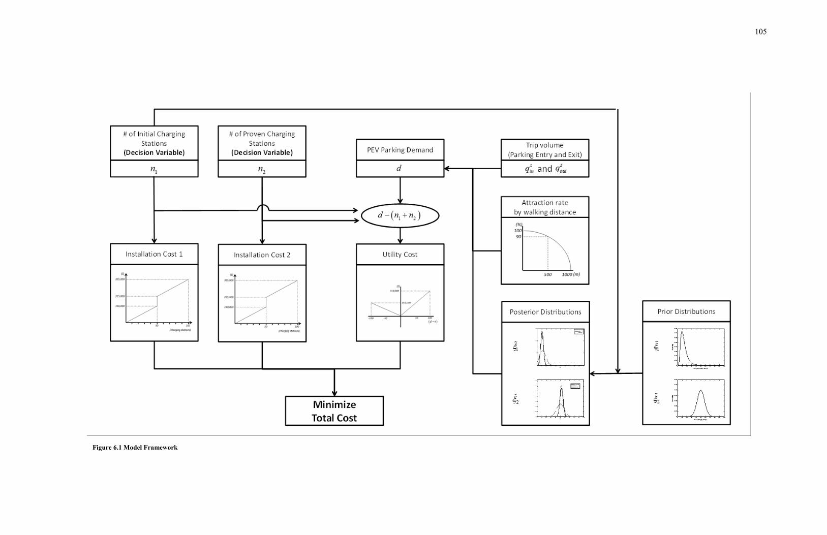
105
Figure 6.1 Model Framework
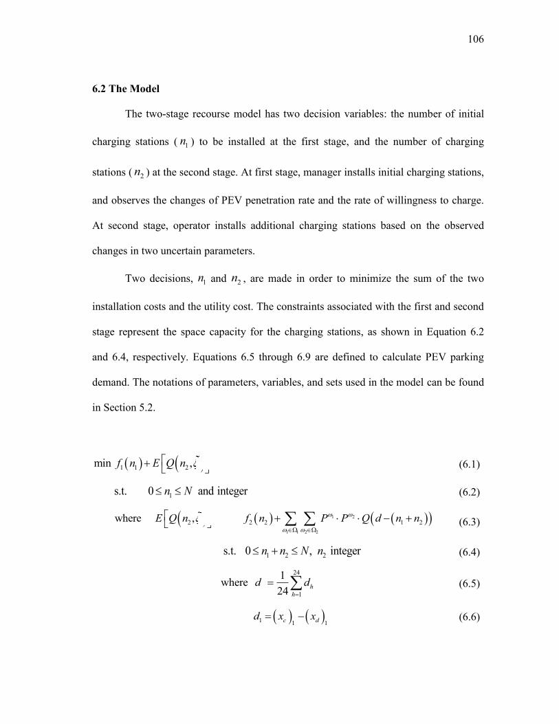
106
6.2 The Model
The two-stage recourse model has two decision variables: the number of initial
charging stations ( 1n ) to be installed at the first stage, and the number of charging
stations ( 2n ) at the second stage. At first stage, manager installs initial charging stations,
and observes the changes of PEV penetration rate and the rate of willingness to charge.
At second stage, operator installs additional charging stations based on the observed
changes in two uncertain parameters.
Two decisions, 1n and 2n , are made in order to minimize the sum of the two
installation costs and the utility cost. The constraints associated with the first and second
stage represent the space capacity for the charging stations, as shown in Equation 6.2
and 6.4, respectively. Equations 6.5 through 6.9 are defined to calculate PEV parking
demand. The notations of parameters, variables, and sets used in the model can be found
in Section 5.2.
1 1 2min ,f n E Q n
(6.1)
1s.t. 0 and integern N (6.2)
1 2
1 1 2 2
2 2 2 1 2where , minE Q n f n P P Q d n n
(6.3)
1 2 2s.t. 0 , integern n N n
(6.4)
24
1
1where
24h
h
d d
(6.5)
1 1 1c dd x x
(6.6)

107
1
2, ,24
h h c dh hd d x x
h
(6.7)
1 2
1, ,24
p
s s
c inh hs N
x q W l
h
(6.8)
1 2
1, ,24
p
s s
d outh hs N
x q W l
h
(6.9)
Random variables, PEV penetration rate, and rate of willingness to charge ( 1
and 2 ) are realized from updated uncertainties, which indicate the posterior
distributions of uncertain parameters. The details of the uncertainty updating process are
described in the next section.
6.3 Decision-Dependent Assessment of Uncertainty
A manager’s decision can influence the uncertainty in parameters. For example,
PEV owners who have seen charging stations installed in parking buildings tend to take
advantage of the charging service. This is similar to product advertisements affecting a
consumer’s choice. The updated uncertainty of a decision is referred to as ‘decision-
dependent assessment of uncertainty’ in this dissertation.
For this model, decision-dependent assessment of uncertainty is evaluated using
Bayesian inference. The updated uncertainty could be obtained in the form of a
probability density function and is evaluated as a posterior distribution in Bayesian
inference. The posterior distribution is derived from prior and likelihood distributions.
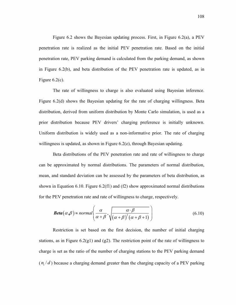
108
Figure 6.2 shows the Bayesian updating process. First, in Figure 6.2(a), a PEV
penetration rate is realized as the initial PEV penetration rate. Based on the initial
penetration rate, PEV parking demand is calculated from the parking demand, as shown
in Figure 6.2(b), and beta distribution of the PEV penetration rate is updated, as in
Figure 6.2(c).
The rate of willingness to charge is also evaluated using Bayesian inference.
Figure 6.2(d) shows the Bayesian updating for the rate of charging willingness. Beta
distribution, derived from uniform distribution by Monte Carlo simulation, is used as a
prior distribution because PEV drivers’ charging preference is initially unknown.
Uniform distribution is widely used as a non-informative prior. The rate of charging
willingness is updated, as shown in Figure 6.2(e), through Bayesian updating.
Beta distributions of the PEV penetration rate and rate of willingness to charge
can be approximated by normal distributions. The parameters of normal distribution,
mean, and standard deviation can be assessed by the parameters of beta distribution, as
shown in Equation 6.10. Figure 6.2(f1) and (f2) show approximated normal distributions
for the PEV penetration rate and rate of willingness to charge, respectively.
2,
1normal
Beta , (6.10)
Restriction is set based on the first decision, the number of initial charging
stations, as in Figure 6.2(g1) and (g2). The restriction point of the rate of willingness to
charge is set as the ratio of the number of charging stations to the PEV parking demand
( 1 /n d ) because a charging demand greater than the charging capacity of a PEV parking

109
building will result in PEV drivers disappointment; hence, the rate of charging
willingness will be reduced. In the same way, the restriction point of the PEV
penetration rate is set as the ratio of the number of charging stations to parking demand.
Likelihood distribution is generated based on the restricted prior distribution by
the Monte Carlo sampling method. Finally, posterior distributions are obtained based on
prior and likelihood distributions, as in Figure 6.2(h1) and (h2). The posterior
distributions show lower variance compared to prior distributions, which indicates that
uncertainty is reduced after Bayesian updating.
6.4 Case Study
In order to demonstrate the CSI-DDAU problem, the CSI project of Texas A&M
University, which was used as a case study in Section 5, was used again. Installation cost,
utility cost, and uncertainties were assumed and defined as the same values in the case
study in Section 5. For the CSI-DDAU problem, the installation cost function for initial
charging stations ( 1f ) was defined as being the same as for additional ones ( 2f ).
The stochastic programming problem with continuous distributions is usually
impossible to solve exactly, so the approximation approach can be used to solve the
problem (Morton and Popova 2004; Mak et al. 1999). To solve the CSI-DDAU problem,
two methods were used: Monte Carlo sampling to generate some observations of the
random parameters and genetic algorithm to find the best combination of decision
variables. Basic GA operators for the case study are defined in Table 6.1.
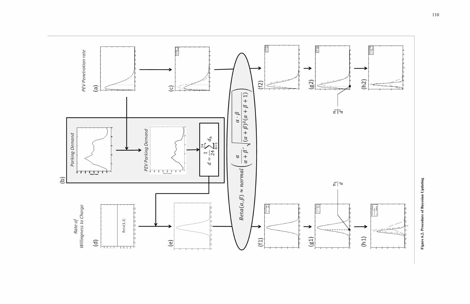
110
Fig
ure
6.2
. P
roce
du
re o
f B
ayes
ian
Up
da
tin
g
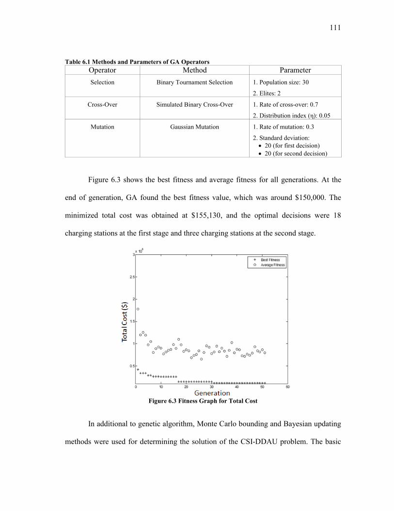
111
Table 6.1 Methods and Parameters of GA Operators
Operator Method Parameter
Selection Binary Tournament Selection 1. Population size: 30
2. Elites: 2
Cross-Over Simulated Binary Cross-Over 1. Rate of cross-over: 0.7
2. Distribution index (η): 0.05
Mutation Gaussian Mutation 1. Rate of mutation: 0.3
2. Standard deviation:
20 (for first decision)
20 (for second decision)
Figure 6.3 shows the best fitness and average fitness for all generations. At the
end of generation, GA found the best fitness value, which was around $150,000. The
minimized total cost was obtained at $155,130, and the optimal decisions were 18
charging stations at the first stage and three charging stations at the second stage.
Figure 6.3 Fitness Graph for Total Cost
In additional to genetic algorithm, Monte Carlo bounding and Bayesian updating
methods were used for determining the solution of the CSI-DDAU problem. The basic
112
information of the algorithm, such as the batch size, the number of batches, and the
sample size, were the same as in the CSI problem.
Table 6.2 shows the computational results of the CSI-DDAU problem. The
analysis results, given the random parameters, indicated that the optimal decisions for
the two stages were 18 charging stations at the first stage and three charging stations at
the second stage. The upper and lower bounds were $156,460 with $4,190 ( =0.95)
and $155,130 with $4,170 ( =0.95). Compared to the results of the CSI problem, the
total cost in the CSI-DDAU problem is higher than that in the CSI problem, and the
number of charging stations in the CSI-DDAU problem is less than that in the CSI
problem. It is expected that these differences result from uncertainty in parameters.
Table 6.2 Results
Optimal Solution (*
1n and *
2n ) 18 and 3
Lower Bound
Batch size 30
Number of batches 30
Point estimate 155,130
Error estimate 4,170
Upper Bound
Sample size 1,000
Point estimate 156,460
Error estimate 4,190
CPU Time (sec) 3,358

113
6.5 Summary
This section presented a charging station installation problem with decision-
dependent assessment of uncertainty. The objective of the CSI-DDAU problem was to
find the optimal number of charging stations at the first and second stages and the
amount of minimum total cost. This section showed how the first decision affects
uncertainty in parameters. The Bayesian updating process gave a posterior distribution
of each parameter, which is the updated uncertainty. Based on the posterior distribution,
the decision at the second stage was made to minimize the total cost.
Monte Carlo bounding, Bayesian updating, and genetic algorithm were used to
solve this CSI-DDAU problem. The analysis results showed a lower number of total
charging stations and higher upper and lower bounds of the total cost compared to the
results of the CSI problem.
114
7. SUMMARY AND CONCLUSIONS
This section summarizes the work and contributions of this research and
discusses limitations. Employed methodologies and recommendations for future research
are also discussed. In the first section, the suggested problems and solution methods in
this research are summarized, along with the contributions of this research. The second
section presents the limitations of the developed methodologies and suggests some
recommendations for future research.
7.1 Overall Summary and Discussion
The major objective of this research was to develop a strategic model to make
optimal decisions for constructing PEV parking buildings and installing charging
stations and to investigate the impact of PEV parking buildings on electric power
systems. The strategic model consists of three problems; PEV parking building problem,
problem for investigating the impact of PEV parking building on electric power system,
and charging station installation problem.
More specifically, the PEV parking building development problem supports the
evaluation of the optimal location of parking buildings and incentive structures to
maximize a developer’s profit, while the charging station installation problem aids
parking building managers in deciding the optimal number of charging stations to be
installed. The work done in this research is reviewed next in terms of the specific
research objectives listed in Section 1.
115
1. Develop a deterministic PEV infrastructure development problem that can be used to
find optimal decisions based on current traffic and power system conditions.
In order to consider the two different systems, a PEV parking building problem
was proposed in the form of a bilevel programming problem. An upper-level BLPP is a
managerial problem that consists of three revenue components, and a lower-level
follower problem of BLPP explains drivers’ behavior. The relationship between a
developer’s decision and drivers’ behavior was formulated in a modified link cost
function in Section 3.
2. Develop a stochastic PEV charging station installation problem that can be used to
decide the optimal number of charging stations to be installed in existing parking
buildings.
A stochastic programming problem was developed to consider uncertainty in
parameters, such as PEV penetration rate and rate of willingness to charge. This
dissertation presented two stochastic programming problems—a two-stage simple
recourse problem and a two-stage recourse problem with decision-dependent assessment
of uncertainty—in Section 5 and Section 6, respectively. In contrast to conventional
stochastic problems, a continuous distribution of random parameters was applied to
consider more various scenarios. In particular, the CSI-DDAU problem in Section 6
116
showed how a manager’s decision affects uncertainty in parameters. The influence was
modeled using the Bayesian updating process.
3. Design meta-heuristic algorithms that can exploit problem structure in solving a
problem and can make it possible to find a near-optimal solution for the proposed
problem within a reasonable run time.
Bilevel programming problems and stochastic programming problems with
continuous distributions are very difficult to solve exactly. To find the best-quality
combination solution, a genetic algorithm was applied to the PEV parking building
problem, CSI problem, and CSI-DDAU problem. The Monte Carlo bounding method
was applied to the CSI problem and CSI-DDAU problem to solve the stochastic
programming problem with continuous distributions.
4. Develop a problem to investigate the impact of PEV infrastructures on transportation
networks and electric power systems.
The impact of a PEV infrastructure on the two systems was investigated in terms
of locational marginal prices. A PEV parking building, in V2G and G2V modes, will
influence a power system’s operating condition as electric generation or load. Change of
LMP was observed by integration of power flow analysis and the PEV parking building

117
problem. The results of the numerical example in Section 4 verified the impact of a PEV
parking building on power system operating conditions and locational marginal prices.
5. Make recommendations that would assist PEV infrastructure developers and managers
in the decision stage regarding construction of a new facility or installation of charging
stations in an existing facility.
Managerial implications and recommendations for PEV parking building
developers and managers were suggested in terms of sensitivity analysis. Walkability
and maximum trip rate showed much influence on a developer’s total revenue, so these
two factors should be considered when developing new PEV parking buildings. In
addition, managers who have a plan to install charging stations in existing parking
buildings should try to reduce the difference between the supply of charging stations and
the PEV charging demand.
7.2 Recommendations for Future Research
Although this study developed beneficial models for PEV parking developers
and managers, the models do not consider all possible scenarios and factors. If PEV
parking buildings and charging stations are to become widespread, many additional
important factors and problems that were not considered in this study need to be
addressed. This section identifies some issues as recommendations for future research.
118
First, the PEV parking charging problem described in Section 3 focused on
deterministic traffic flows. The problem can be extended to account for uncertainty,
where the trips are considered as cross-correlated stochastic processes. Deterministic
equilibrium assignment for traffic flow assumes that drivers have perfect information,
which is not real. The stochastic process can relax the assumption of perfect information.
Second, in the PEV parking building problem detailed in Section 3, sensitivity of
the demand based on the incentive parameter ( ) was assumed, not estimated from
surveys. A more realistic value of the incentive parameter could be obtained using
surveys.
Third, other potential revenue models (e.g., charging service, carbon credit
trading, and outage management service) or initial cost models (e.g., capital cost and real
estate cost) could be added to the PEV parking building problem.
Fourth, in the PEV parking building problem, the model extension that considers
capital and location-specific real estate costs can ultimately be used to determine an
investment decision. This can be done on an ad hoc basis or if the costs show some
structure with respect to network links, via cost functions.
Fifth, the CSI problem and CSI-DDAU problem in this study focused on
installation of charging stations in a fixed parking building. The problems can be
extended to a capacitated facility location problem and multiple facilities location
problem. The future problems would make the CSI and CSI-DDAU problems more open
and flexible.

119
Finally, utility cost of a parking building manager was identified as the most
sensitive factor in the CSI and CSI-DDAU problems. Therefore, to obtain more realistic
results, a more accurate utility cost function needs to be defined by surveys.
120
REFERENCES
Abdulaal, M. and Leblanc, L.J. (1979). “Continuous equilibrium network design models.”
Transportation Research Part B, 13B, 19-32.
Axsen, J. and Kurani, K.S. (2008). The Early U.S. Market for PHEVs: Anticipating
Consumer Awareness, Recharge Potential, Design Priorities and Energy Impacts.
Institute of Transportation Studies, University of California, Davis.
Balducci, P.J. (2008). Plug-in Hybrid Electric Vehicle Market Penetration Scenarios.
Pacific Northwest national Laboratory.
Beale, E.M.L. (1955). "On minimizing a convex function subject to linear inequalities."
Journal of Royal Statistical Society. B17, 173-184.
Beckmann, M., McGuire, G.B., and Winstern, C.B. (1956). Studies in the Economics of
Transportation. Yale University Press, New Haven.
Birge, J.R. and Rosa, C.H. (1995). "Modelling investment uncertainty in the costs of
global CO2 emission policy." European Journal of Operations Research, 83,
466–488.
Bureau of Public Roads (BPR) (1964). Traffic Assignment Manual. US Department of
Commerce, Urban Planning Divisions, Washington, DC (20230).
Carino, D.R., Kent, T., Meyers, D.H., Stacy, C., Sylvanus, M., Turner, A.L., Watanabe,
K., and Ziemba, W.T. (1994). "The Russel- Yasuda Kasai Model: An

121
asset/liability model for a Japanese insurance company using multistage
stochastic programming." Interfaces, 24(1), 29-49.
Cooper, L. (1963). “Location–allocation problems.” Operations Research, 11, 331–343.
Dantzig, G.B. (1955). "Linear programming under uncertainty." Management Science, 1,
197-206.
Davis, G.A. (1994). “Exact local solution of continuous network design problem via
stochastic user equilibrium assignment.” Transportation Research Part B,
28B(1), 61-75.
Denholm, P. and Short, W. (2006). An Evaluation of Utility System Impacts and Benefits
of Optimally Dispatched Plug-in Hybrid Electric Vehicles. National Renewable
Energy Laboratory (NREL), Golden, CO.
Ergűn, G. (1971). "Development of a Downtown Parking Model." Highway Research
Record, 369, 118-134.
Fell, K., Huber, K., Zink, B., and others. (2010). Assessment of plug-in electric vehicle
integration with ISO/RTO Systems. Technical report, ISO/RTO Council.
Fisk, C.S. (1984). “Game theory and transportation systems modeling.” Transportation
Research Part B, 18B(4), 301-313.
Fox, H. and Associates (1994). User Guide to PEDROUTE 3.15. Halcrow Fox, London.
122
Frantzeskakis, L. and Powell, W.B. (1990). "A successive linear approximation
procedure for stochastic, dynamic vehicle allocation problems." Transportation
Science, 24, 40–57.
Friesz, T.L., Cho, H., Mehta, N.J., Tobin, R.L., and Anandalingam, G. (1992). “A
simulated annealing approach to the network design problem with variational
inequality constraints.” Transportation Science, 26(1), 18-26.
Garcia, R. and Marin, A. (2002). “Parking capacity and pricing in park’n ride trips: A
continuous equilibrium network design problem.” Annals of operations research,
116, 153-178.
Goldman, A.J. (1971). “Optimal center location in simple networks.” Transportation
Science, 5, 212–221.
Guille, C. and Gross, G. (2009). “A conceptual framework for the vehicle-to-grid (V2G)
implementation.” Energy Policy, 37(11), 4379-4390.
Hadley, S.W. and Tsvetkova, A. (2008). Potential Impact of Plug-in Hybrid Electric
Vehicles on Regional Power Generation. Oak Ridge National Laboratory, Oak
Ridge, TN.
Hansen, P., Jaumard, B., and Savard, G. (1992). “New branch and bound rules for linear
bilevel programming.” SIAM Journal on Scientific and Statistical Computing, 13,
1194-1217.
123
Harvey, S. and Hogan, W.W. (2000). Nodal and zonal congestion management and the
exercise of market power, Center for Business and Government. John F.
Kennedy School of Government, Harvard University, Cambridge, MA.
Hess, P.M., Moudon, A.V., Snyder, M.C., and Stanilov, K. (1999). “Site design and
pedestrian travel.” Transportation Research Record: Journal of the
Transportation Research Board, 1674, 9-19.
Hoogendoorn, S.P. and Bovy, P.H.L. (2004). “Pedestrian route-choice and activity
scheduling theory and models.” Transportation Research Part B:
Methodological, 38(2), 169-190.
Hunt, J.D. (1988). "Parking location choice: Insights and representations based on
observed behaviour and hierarchical logit modelling formulation." Paper
presented to the 5th Annual Meeting of the Institute of Transportation Engineers,
Vancouver.
Kempton, W. (2007). "Vehicle to grid power." Workshop at IEEE Conference,
Washington DC, September.
Kempton, W. and Dhanju, A. (2006). “Electric vehicles with V2G: Storage for
largescale wind power.” Windtech Int, 2(2), 18-21.
Kempton, W., and Tomic, J. (2005a). “Vehicle-to-grid power implementation: From
stabilizing the grid to supporting large-scale renewable energy.” Journal of
Power source. 144(1), 280-294.

124
Kempton, W. and Tomic, J. (2005b). “Vehicle-to-grid power fundamentals: Calculating
capacity and net revenue.” Journal of Power source, 144(1), 268-279.
Ker, I. and Ginn, S. (2003). Myths and realities in walkable catchments: The case of
walking and transit.
<findarticles.com/p/articles/mi_qa3927/is_200306/ai_n9255068> (July 26, 2011)
Kolstad, C.D. (1985). A Review of the Literature on Bi-Level Mathematical
Programming. Report LA-10284-MS, Los Alamos National Laboratory, Los
Alamos, NM.
Labbe’, M. and Marcotte, P., and Savard, G. (1998). "A bilevel model of taxation and its
application to optimal highway pricing." Management Science, 44(12), 1608-
1622.
Lam, W.H.K., Li, Z., Huang, H., and Wong, S.C. (2006). "Modeling time-dependent
travel choice problems in road networks with multiple user classes and multiple
parking facilities." Transportation Research part B, 40, 368-395.
Lambe, T.A. (1996). "Driver choice of parking in the city." Socio. Econ. Plann. Sci.,
30(3), 207-219.
Landis, B.W., Vattikuti, V.R., Ottenberg, R.M., McLeod, D.S., and Guttenplan, M.
(2001). “Modeling the roadside walking environment: Pedestrian level of service.”
Transportation Research Record: Journal of the Transportation Research Board,
1663, 82-88.

125
LeBlanc, L.J. (1975). "An algorithm for the discrete network design problem."
Transportation Science, 9, 183-199.
Lilienthal, P. and Brown, H. (2007). Potential carbon emissions reductions from plug-in
hybrid electric vehicles by 2030, National Renewable Energy Laboratory
(NREL), Golden, CO.
Litman, T.A. (2003). “Economic value of walkability.” Transportation Research Record:
Journal of the Transportation Research Board, 1828, 3-11.
Louie, H. and Strunz, K. (2008). "Locational Marginal Princing in North American
Power Systems." ETG-Fachbericht-Netzregelung und Systemfűhrung, Műnchen,
Germany.
Mak, W., Morton, D.P., and Wood, R.K. (1999), "Monte Carlo bounding techniques for
determining solution quality in stochastic programs." Operations Research
Letters, 24, 47-56.
Marcotte, P. (1983). “Network optimization with continuous control parameters,”
Transportation Science, 17(2), 181-197.
Matley, T.M., Goldman, L.M., and Fineman, B.J. (2000). “Pedestrian travel potential in
Northern New Jersey: A metropolitan planning organization’s approach to
identifying investment priorities.” Transportation Research Record: Journal of
the Transportation Research Board, 1705, 1-8.
Mitchell, M. (1998). An introduction to genetic algorithms, MIT Press, Cambridge, MA.

126
Morton, D.P. and Popova, E. (2004). “A Bayesian stochastic programming approach to
an employee scheduling problem.” IIE Transactions, 36, 155-167.
Mulvey, J.M. and Vladimirou H. (1991). "Applying the progressive hedging algorithm
to stochastic generalized networks." Annals of Operations Research, 31, 399-424.
Ott, A.L. (2003). "Experience with PJM market operation, system design, and
implementation." IEEE Transactions on Power Systems, 18(2), 528-534.
Parks, K., Denholm, P., and Markel, T. (2007). Costs and Emissions Associated with
Plug-in Hybrid Electric Vehicle Charging in the Xcel Energy Colorado Service
Territory. National Renewable Energy Laboratory (NREL), Golden, CO.
Pereira, M.V.F and Pinto, L.M.V.G. (1991). "Multi-stage stochastic optimization applied
to energy planning." Mathematical Programming, 52, 359-375.
Pierce Jr, H.E., Colborn, H.W., Coleman, D.W., Marriage, E.A., Richard, J.C., Rindt,
L.J., Rubino, L.J., Stagg, G.W., Traub, T.P., Vandergrift, J., and others (1973).
"Common format for exchange of solved load flow data." IEEE Transactions on
Power Apparatus and Systems, 92(6), 1916-1925.
Pisarski, A.E. (2006). Commuting in America III: The Third National Report on
Commuting Patterns and Trends. Transportation Research Board of the National
Academies, Washington, DC.
Plastria, F. (1987). “Solving general continuous single facility location problems by
cutting planes.” European Journal of Operational Research, 29(1), 98-110.
127
Powell, W.B. (1990). "Real-time optimization for truckload motor carriers." OR/MS
Today, 17(2), 28–33.
Saadat, H. (2002). Power System Analysis, McGraw-Hill, New York.
Short, W. and Denholm, P. (2006). A Preliminary Assessment of Plug-in Hybrid Electric
Vehicles on Wind Energy Markets. National Renewable Energy Laboratory,
Golden, CO.
Solomon, J. and Vincent, R. (2003). Development and Evaluation of a Plug-in HEV with
Vehicle-to-grid Power Flow. California Air Resources Board, Sacramento, CA.
Southworth, M. (2005). “Designing the walkable city.” Journal of Urban Planning and
Development, 131(4), 246-257.
Stovall, T.K., Hadley, S.W. and Rizy, D.T. (2005). “Distributed generation: Who
benefits?” Public Utilities Fortnightly, 34-38, March.
Sullivan, J.L., Salmeen, I.T., and Simon, C.P. (2009). PHEV Marketplace Penetration:
An Agent Based Simulation. University of Michigan, Ann Arbor, Transportation
Research Institute.
Takriti, S., Birge, J.R., and Long, E. (1995). "A stochastic model for the unit
commitment problem." IEEE Transactions on Power Systems, 11(3), 1497-1508.
Tam, M.L. and Lam, W.H.K. (2000). “Maximum car ownership under constraints of
road capacity and parking space.” Transportation Research Part A, 34, 145-170.

128
Tatsumi, H. (2003). "Modeling of parking lot choice behavior for traffic simulation."
Journal of the Eastern Asia Society for Transportation Studies, 5, 2077-2091.
Tong, C.O., Lau, W.W.T, and Wong, S.C. (2004). "A demand-supply equilibrium model
for parking services in hong kong." Transactions-Hong Kong Institution of
Engineers, 11(1), 48-53.
U.S. Energy Information Administration (2009). Annual energy outlook 2009: With
projection to 2030.
http://www.eia.gov/oiaf/aeo/pdf/0383(2009).pdf
Wardrop, J.G. (1952). “Some theoretical aspects of road traffic research.” Proceedings
of the Institution of Civil Engineers Part II, 1, 325-378.
Weber, A. (1909). Ü ber den standort der industrien. JCB Mohr, Tübingen.
Yang, H. and Bell, M.G.H. (1997), “Traffic restraint, road pricing and network
equilibrium.” Transportation Research Park B, 31(4), 303-314.
Zhichun, L., Jaijun, H., Lam, W.H.K., and Wong, S.C. (2007). “Optimization of time-
varying parking charges and parking supply in networks with multiple user classes
and multiple parking facilities.” Tsinghua Science and Technology, 12(2), 167-177.
Ziliaskopoulos, A.K. (2000). "A linear programming model for the single destination
system optimum dynamic traffic assignment problem." Transportation Science,
34(1), 37-49.

129
Zimmerman, R.D., Murillo-Sanchez, C.E., and Thomas, R.J. (2011). “Matpower: Steady
state operations, planning and analysis tools for power systems research and
education." IEEE Transactions on Power Systems, 26(1), 12-19.
130
APPENDIX I
NOTATION OF DYNAMIC TRAFFIC ASSIGNMENT
k = density
v
= link free flow speed
w
= backward propagation speed
C = the set of cells: ordinary ( OC ), diverging ( DC ), merging ( MC ),
source ( RC ), and sink ( SC )
T = the set of discrete time intervals t
ix = the number of vehicles in cell i at time interval t t
iN = the maximum number of vehicles in cell i at time interval t
t
ijy = the number of vehicles moving from cell i to cell j at time interval
t
E = the set of cell connectors: ordinary ( OE ), diverging ( DE ), merging
( ME ), source ( RE ), and sink ( SE )
t
iQ = the maximum number of vehicles that can flow into or out of cell i during time interval t
t
i = ratio /v w for each cell and time interval
i
= the set of successor cells to i
1 i = the set of predecessor cells to i t
id = demand (inflow) at cell i in time interval t

131
APPENDIX II
MATRIX OF DEMAND FOR TRIPS

132
APPENDIX III
COST FUNCTION PARAMETERS
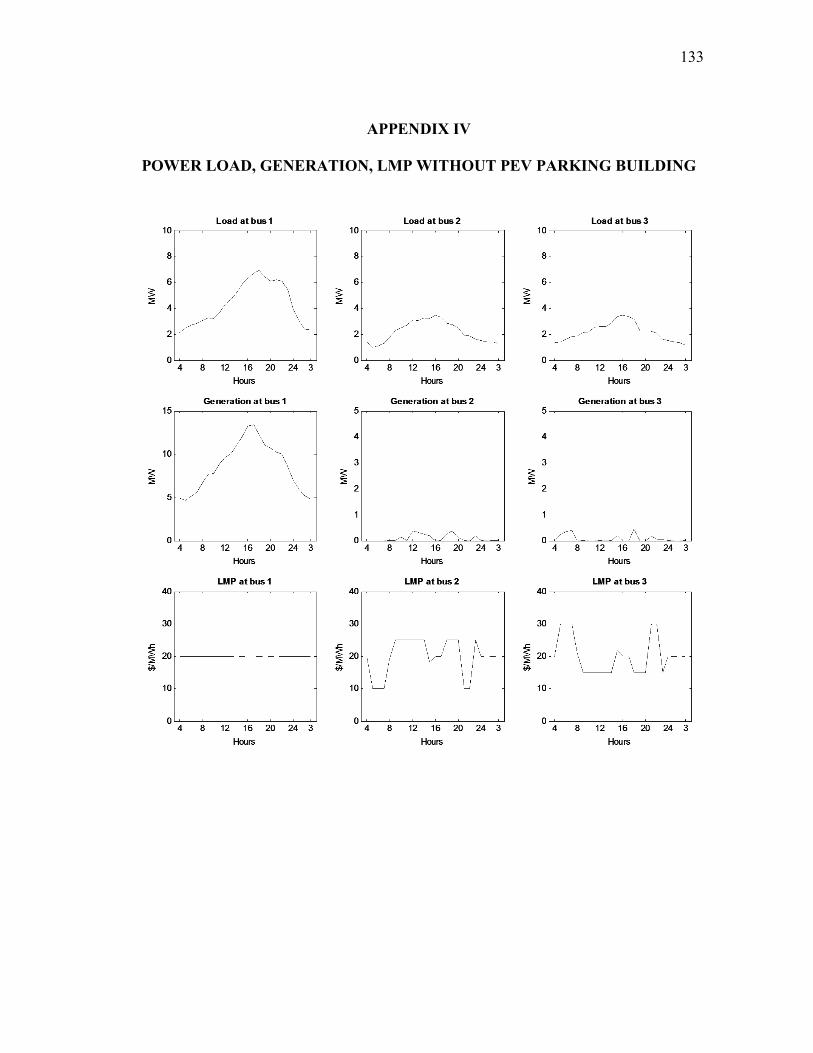
133
APPENDIX IV
POWER LOAD, GENERATION, LMP WITHOUT PEV PARKING BUILDING
134
APPENDIX V
NOTATION OF DATA FORMAT
Generator Data Format
bus = bus number
Pg = real power output (MW)
Qg = reactive power output (MVAr)
Qmax = maximum reactive power output (MVAr)
Qmin = minimum reactive power output (MVAr)
Vg = voltage magnitude setpoint (p.u.)
mBase = total MVA base of this machine, defaults to baseMVA
status = > 0 – machine in service
≤ 0 – machine out of service
Pmax = maximum real power output (MW)
Pmin = minimum real power output (MW)
Branch Data Format
fbus = from bus number
tbus = to bus number
r = resistance (p.u.)
x = reactance (p.u.)
b = total line charging susceptance (p.u.)
rateA = MVA rating A (long term rating)
rateB = MVA rating B (short term rating)
rateC = MVA rating C (emergency rating)
ratio = transformer off nominal turns ratio (= 0 for lines)
angle = transformer phase shift angle (degrees)
status = 1 – in service
0 – out of service
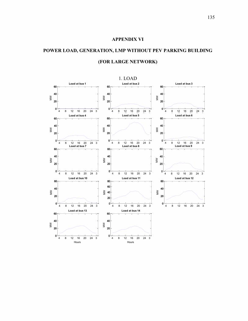
135
APPENDIX VI
POWER LOAD, GENERATION, LMP WITHOUT PEV PARKING BUILDING
(FOR LARGE NETWORK)
1. LOAD
4 8 12 16 20 24 30
20
40
60
0
20
40
60Load at bus 1
MW
4 8 12 16 20 24 30
20
40
60
0
20
40
60Load at bus 2
MW
4 8 12 16 20 24 30
20
40
60
0
20
40
60Load at bus 3
MW
4 8 12 16 20 24 30
20
40
60
0
20
40
60Load at bus 4
MW
4 8 12 16 20 24 30
20
40
60
0
20
40
60Load at bus 5
MW
4 8 12 16 20 24 30
20
40
60
0
20
40
60Load at bus 6
MW
4 8 12 16 20 24 30
20
40
60
0
20
40
60Load at bus 7
MW
4 8 12 16 20 24 30
20
40
60
0
20
40
60Load at bus 8
MW
4 8 12 16 20 24 30
20
40
60
0
20
40
60Load at bus 9
MW
4 8 12 16 20 24 30
20
40
60
0
20
40
60Load at bus 10
MW
4 8 12 16 20 24 30
20
40
60
80
0
20
40
60
80Load at bus 11
Hours
MW
4 8 12 16 20 24 30
20
40
60
0
20
40
60Load at bus 12
Hours
MW
4 8 12 16 20 24 30
20
40
60
0
20
40
60Load at bus 13
Hours
MW
4 8 12 16 20 24 30
20
40
60
0
20
40
60Load at bus 14
Hours
MW
4 8 12 16 20 24 30
20
40
60
0
20
40
60Load at bus 1
MW
4 8 12 16 20 24 30
20
40
60
0
20
40
60Load at bus 2
MW
4 8 12 16 20 24 30
20
40
60
0
20
40
60Load at bus 3
MW
4 8 12 16 20 24 30
20
40
60
0
20
40
60Load at bus 4
MW
4 8 12 16 20 24 30
20
40
60
0
20
40
60Load at bus 5
MW
4 8 12 16 20 24 30
20
40
60
0
20
40
60Load at bus 6
MW
4 8 12 16 20 24 30
20
40
60
0
20
40
60Load at bus 7
MW
4 8 12 16 20 24 30
20
40
60
0
20
40
60Load at bus 8
MW
4 8 12 16 20 24 30
20
40
60
0
20
40
60Load at bus 9
MW
4 8 12 16 20 24 30
20
40
60
0
20
40
60Load at bus 10
MW
4 8 12 16 20 24 30
20
40
60
80
0
20
40
60
80Load at bus 11
Hours
MW
4 8 12 16 20 24 30
20
40
60
0
20
40
60Load at bus 12
Hours
MW
4 8 12 16 20 24 30
20
40
60
0
20
40
60Load at bus 13
Hours
MW
4 8 12 16 20 24 30
20
40
60
0
20
40
60Load at bus 14
HoursM
W
4 8 12 16 20 24 30
20
40
60
0
20
40
60Load at bus 1
MW
4 8 12 16 20 24 30
20
40
60
0
20
40
60Load at bus 2
MW
4 8 12 16 20 24 30
20
40
60
0
20
40
60Load at bus 3
MW
4 8 12 16 20 24 30
20
40
60
0
20
40
60Load at bus 4
MW
4 8 12 16 20 24 30
20
40
60
0
20
40
60Load at bus 5
MW
4 8 12 16 20 24 30
20
40
60
0
20
40
60Load at bus 6
MW
4 8 12 16 20 24 30
20
40
60
0
20
40
60Load at bus 7
MW
4 8 12 16 20 24 30
20
40
60
0
20
40
60Load at bus 8
MW
4 8 12 16 20 24 30
20
40
60
0
20
40
60Load at bus 9
MW
4 8 12 16 20 24 30
20
40
60
0
20
40
60Load at bus 10
MW
4 8 12 16 20 24 30
20
40
60
80
0
20
40
60
80Load at bus 11
Hours
MW
4 8 12 16 20 24 30
20
40
60
0
20
40
60Load at bus 12
Hours
MW
4 8 12 16 20 24 30
20
40
60
0
20
40
60Load at bus 13
Hours
MW
4 8 12 16 20 24 30
20
40
60
0
20
40
60Load at bus 14
Hours
MW
4 8 12 16 20 24 30
20
40
60
0
20
40
60Load at bus 1
MW
4 8 12 16 20 24 30
20
40
60
0
20
40
60Load at bus 2
MW
4 8 12 16 20 24 30
20
40
60
0
20
40
60Load at bus 3
MW
4 8 12 16 20 24 30
20
40
60
0
20
40
60Load at bus 4
MW
4 8 12 16 20 24 30
20
40
60
0
20
40
60Load at bus 5
MW
4 8 12 16 20 24 30
20
40
60
0
20
40
60Load at bus 6
MW
4 8 12 16 20 24 30
20
40
60
0
20
40
60Load at bus 7
MW
4 8 12 16 20 24 30
20
40
60
0
20
40
60Load at bus 8
MW
4 8 12 16 20 24 30
20
40
60
0
20
40
60Load at bus 9
MW
4 8 12 16 20 24 30
20
40
60
0
20
40
60Load at bus 10
MW
4 8 12 16 20 24 30
20
40
60
80
0
20
40
60
80Load at bus 11
Hours
MW
4 8 12 16 20 24 30
20
40
60
0
20
40
60Load at bus 12
HoursM
W
4 8 12 16 20 24 30
20
40
60
0
20
40
60Load at bus 13
Hours
MW
4 8 12 16 20 24 30
20
40
60
0
20
40
60Load at bus 14
Hours
MW

136
2. GENERATION

137
3. LMP
4 8 12 16 20 24 30
20
40
60
0
20
40
60LMP at bus 1
$/M
Wh
4 8 12 16 20 24 30
20
40
60
0
20
40
60LMP at bus 2
$/M
Wh
4 8 12 16 20 24 30
20
40
60
0
20
40
60LMP at bus 3
$/M
Wh
4 8 12 16 20 24 30
20
40
60
0
20
40
60LMP at bus 4
$/M
Wh
4 8 12 16 20 24 30
20
40
60
0
20
40
60LMP at bus 5
$/M
Wh
4 8 12 16 20 24 30
20
40
60
0
20
40
60LMP at bus 6
$/M
Wh
4 8 12 16 20 24 30
20
40
60
0
20
40
60LMP at bus 7
$/M
Wh
4 8 12 16 20 24 30
20
40
60
0
20
40
60LMP at bus 8
$/M
Wh
4 8 12 16 20 24 30
20
40
60
0
20
40
60LMP at bus 9
$/M
Wh
4 8 12 16 20 24 30
20
40
60
0
20
40
60LMP at bus 10
$/M
Wh
4 8 12 16 20 24 30
20
40
60
0
20
40
60LMP at bus 11
Hours
$/M
Wh
4 8 12 16 20 24 30
20
40
60
0
20
40
60LMP at bus 12
Hours
$/M
Wh
4 8 12 16 20 24 30
20
40
60
0
20
40
60LMP at bus 13
Hours
$/M
Wh
4 8 12 16 20 24 30
20
40
60
0
20
40
60LMP at bus 14
Hours
$/M
Wh
4 8 12 16 20 24 30
20
40
60
0
20
40
60LMP at bus 1
$/M
Wh
4 8 12 16 20 24 30
20
40
60
0
20
40
60LMP at bus 2
$/M
Wh
4 8 12 16 20 24 30
20
40
60
0
20
40
60LMP at bus 3
$/M
Wh
4 8 12 16 20 24 30
20
40
60
0
20
40
60LMP at bus 4
$/M
Wh
4 8 12 16 20 24 30
20
40
60
0
20
40
60LMP at bus 5
$/M
Wh
4 8 12 16 20 24 30
20
40
60
0
20
40
60LMP at bus 6
$/M
Wh
4 8 12 16 20 24 30
20
40
60
0
20
40
60LMP at bus 7
$/M
Wh
4 8 12 16 20 24 30
20
40
60
0
20
40
60LMP at bus 8
$/M
Wh
4 8 12 16 20 24 30
20
40
60
0
20
40
60LMP at bus 9
$/M
Wh
4 8 12 16 20 24 30
20
40
60
0
20
40
60LMP at bus 10
$/M
Wh
4 8 12 16 20 24 30
20
40
60
0
20
40
60LMP at bus 11
Hours
$/M
Wh
4 8 12 16 20 24 30
20
40
60
0
20
40
60LMP at bus 12
Hours
$/M
Wh
4 8 12 16 20 24 30
20
40
60
0
20
40
60LMP at bus 13
Hours
$/M
Wh
4 8 12 16 20 24 30
20
40
60
0
20
40
60LMP at bus 14
Hours
$/M
Wh
138
VITA
Name: Seok Kim
Address: Civil Engineering Department
c/o Dr. Ivan Damnjanovic
Texas A&M University
College Station, TX 77843-3136
Email Address: [email protected]
Education: B.S., Civil Engineering, Chung-Ang University, 2004
M.S., Civil Engineering, Chung-Ang University, 2006
Ph.D., Civil Engineering, Texas A&M University, 2011