models and methods for automated material identification

2706 IEEE TRANSACTIONS ON GEOSCIENCE AND REMOTE SENSING, VOL. 37, NO. 6, NOVEMBER 1999

Models and Methods for AutomatedMaterial Identification in Hyperspectral

Imagery Acquired Under UnknownIllumination and Atmospheric Conditions

Glenn Healey,Senior Member, IEEE, and David Slater

Abstract—The spectral radiance measured by an airborneimaging spectrometer for a material on the Earth’s surfacedepends strongly on the illumination incident of the materialand the atmospheric conditions. This dependence has limitedthe success of material-identification algorithms that rely onhyperspectral image data without associated ground-truth infor-mation. In this paper, we use a comprehensive physical modelto show that the set of observed 0.4–2.5��m spectral-radiancevectors for a material lies in a low-dimensional subspace of thehyperspectral-measurement space. The physical model capturesthe dependence of the reflected sunlight, reflected skylight, andpath-radiance terms on the scene geometry and on the distri-bution of atmospheric gases and aerosols over a wide rangeof conditions. Using the subspace model, we develop a localmaximum-likelihood algorithm for automated material identifi-cation that is invariant to illumination, atmospheric conditions,and the scene geometry. The algorithm requires only the spectralreflectance of the target material as input. We show that thelow dimensionality of material subspaces allows for the robustdiscrimination of a large number of materials over a widerange of conditions. We demonstrate the invariant algorithmfor the automated identification of material samples in HYDICEimagery acquired under different illumination and atmosphericconditions.

Index Terms—Atmospheric correction, hyperspectral, invari-ant, material identification, HYDICE.

I. INTRODUCTION

A IRBORNE imaging spectrometers provide measurementsover hundreds of contiguous spectral bands at each image

location. The Hyperspectral Digital Imagery Collection Exper-iment (HYDICE) [2] and the airborne visible/infrared imagingspectrometer (AVIRIS) [39] each collect more than two hun-dred spectral bands over the visible through short-wave in-frared wavelengths (0.4–2.5m). This spectral range capturesa large majority of reflected solar radiation while receivinga negligible contribution from thermal emission. Significanteffort has been dedicated to calibrating imaging-spectrometer

Manuscript received October 13, 1998; revised May 25, 1999. This workwas supported in part by the Air Force Office of Scientific Research, AirForce Research Laboratory, and by the Defense Advanced Research ProjectsAgency under Grant F49620-97-1-0492.

The authors are with the Department of Electrical and Computer Engineer-ing, University of California, Irvine, CA 92697 (e-mail: [email protected];[email protected]).

Publisher Item Identifier S 0196-2892(99)07855-9.

output to absolute spectral radiance to allow spectral measure-ments to be directly related to physical variables [1], [5], [15].The high-spectral dimensionality of imaging-spectrometer dataprovides the opportunity to discriminate many materials thatcannot be discriminated using sensors with fewer spectralbands [13].

The identification of materials in calibrated imaging-spectrometer data is complicated by spatial and temporalvariation in illumination and atmospheric conditions. Thisvariation can cause large variability in the measured spectralradiance for a fixed material as conditions change. Thedesire to relate airborne spectrometer data to intrinsic surfaceproperties has led to the development of atmospheric-correction algorithms that attempt to recover surface-spectralreflectance from sensor-spectral radiance. The availabilityof ground-truth data corresponding to the airborne imageryfacilitates atmospheric correction. The empirical-line method[7], for example, uses a set of ground targets of knownreflectance to derive a relationship between sensor-spectralradiance and scene-spectral reflectance. Other techniques(e.g., [11] and [27]), normalize spectra in the scene usingan average-scene spectrum to correct for atmospheric effects.This approach is similar to the retinex algorithm [29] andsuffers from the limitation that the normalized spectrum fora fixed material can be quite sensitive to the distributionof materials in the scene [4]. Model-based approaches[12], [16] express sensor radiance in terms of parametricreflectance and atmospheric models in order to estimatethe unknown parameters across an image. Although model-based approaches eliminate the need for ground-truth data,they are computationally intensive and the complexity of theunderlying models necessitates simplifying assumptions thatlimit accuracy. In addition, atmospheric-correction algorithmstypically assume that direct solar radiation is the dominantcontributor to ground-surface illumination. This assumptionrenders these methods of limited use in less restrictive-illumination environments.

Substantial progress has been made on computational color-constancy algorithms that recover intrinsic surface descriptionsfrom three-band visible color images obtained under unknownillumination conditions [18], [19]. Many of these algorithmsare based on the assumption of low-dimensional linear models

0196–2892/99$10.00 1999 IEEE

HEALEY AND SLATER: MODELS AND METHODS FOR AUTOMATED MATERIAL IDENTIFICATION 2707

for spectral reflectance and illumination functions. The spectraldistribution of outdoor illumination has at least three degreesof freedom [24], [37]. Consequently, the set of observedspectral-radiance functions for a single reflecting material is atleast three-dimensional (3-D). As a result, the sets of possiblethree-band spectral measurements for different materials willoften intersect. Thus, any method for illumination-invariantmaterial identification that uses only the three-band spectralmeasurement at a single spatial location will be unreliable.This difficulty has led to color-constancy algorithms thatutilize information over image regions that contain severalmaterials or observable texture (e.g., [20]–[22], [31]). Thesealgorithms, however, often have difficulty identifying smallmaterial samples or processing regions with spatially nonuni-form illumination.

Airborne-imaging spectrometers afford the possibility thatmethods can be developed for reliable material identificationover a wide range of conditions using only the spectral vectormeasured at a single image location. The success of thesemethods requires that the spectral dimensionality of the sensordata exceeds the dimensionality of the set of spectral-radiancevectors that can be obtained for a single material as conditionschange. In this paper, we use physical models for illuminationand atmospheric variation to examine the sets of 0.4–2.5mspectral-radiance vectors that will be measured for differentmaterials by an airborne sensor. A physical model for sensorspectral radiance is used in conjunction with the MODTRAN3.5 atmospheric-modeling program [3] to generate the sets ofspectral vectors. The analysis shows that over a comprehensiverange of conditions, the set of observed spectral-radiance vec-tors for a material can be represented accurately using a linearmodel with fewer than ten parameters. This result is used toshow that a large set of materials can be discriminated reliablyover a wide range of conditions using imaging-spectrometerdata. Based on the analysis, we derive a maximum-likelihoodalgorithm for automated material identification that is invariantto illumination and atmospheric variation. The algorithm isdemonstrated for the identification of a set of material samplesin HYDICE imagery acquired under different conditions.

II. M OTIVATION

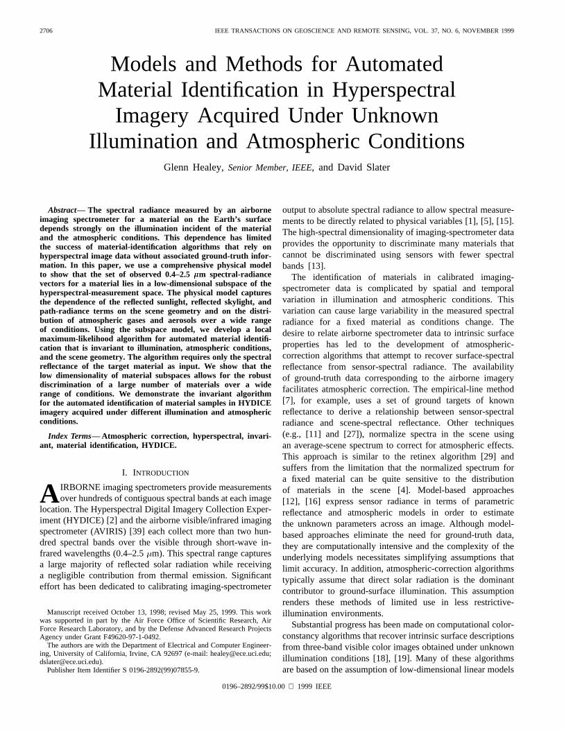
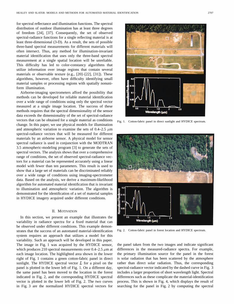
In this section, we present an example that illustrates thevariability in radiance spectra for a fixed material that canbe observed under different conditions. This example demon-strates that the success of an automated material-identificationsystem requires an approach that utilizes a model for thisvariability. Such an approach will be developed in this paper.The image in Fig. 1 was acquired by the HYDICE sensor,which produces 210 spectral measurements over 0.4–2.5m ateach image location. The highlighted area shown in the lowerright of Fig. 1 contains a green cotton-fabric panel in directsunlight. The HYDICE spectral vector for a pixel on thepanel is plotted in the lower left of Fig. 1. On a different day,the same panel has been moved to the location in the forestindicated in Fig. 2, and the corresponding HYDICE spectralvector is plotted in the lower left of Fig. 2. The two curvesin Fig. 3 are the normalized HYDICE spectral vectors for

Fig. 1. Cotton-fabric panel in direct sunlight and HYDICE spectrum.

Fig. 2. Cotton-fabric panel in forest location and HYDICE spectrum.

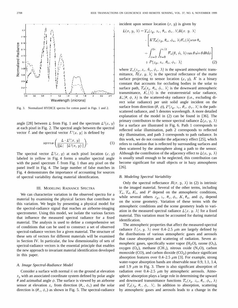
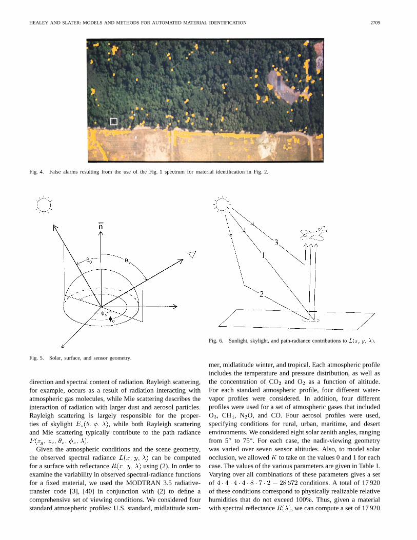
the panel taken from the two images and indicate significantdifferences in the measured-radiance spectra. For example,the primary illumination source for the panel in the forestis solar radiation that has been scattered by the atmosphererather than direct solar radiation. Thus, the correspondingspectral-radiance vector indicated by the dashed curve in Fig. 3includes a larger proportion of short wavelength light. Spectraldifferences such as these complicate the material-identificationprocess. This is shown in Fig. 4, which displays the result ofsearching for the panel in Fig. 2 by computing the spectral


Fig. 3. Normalized HYDICE spectra for cotton panel in Figs. 1 and 2.

angle [28] between from Fig. 1 and the spectrumat each pixel in Fig. 2. The spectral angle between the spectralvector and the spectral vector is defined by

(1)

The spectral vector at each pixel location ( )labeled in yellow in Fig. 4 forms a smaller spectral anglewith the panel spectrum from Fig. 1 than any pixel on thepanel itself in Fig. 4. The large number of false matches inFig. 4 demonstrates the importance of accounting for sourcesof spectral variability during material identification.

III. M ODELING RADIANCE SPECTRA

We can characterize variation in the observed spectra for amaterial by examining the physical factors that contribute tothis variation. We begin by presenting a physical model forthe spectral-radiance signal that reaches an airborne-imagingspectrometer. Using this model, we isolate the various factorsthat influence the measured spectral radiance for a fixedmaterial. The analysis is used to define a comprehensive setof conditions that can be used to construct a set of observedspectral-radiance vectors for a given material. The structure ofthese sets of vectors for different materials will be examinedin Section IV. In particular, the low dimensionality of sets ofspectral-radiance vectors is the essential principle that enablesthe new approach to invariant material identification developedin this paper.

A. Image Spectral-Radiance Model

Consider a surface with normalon the ground at elevationwith an associated coordinate system defined by polar angle

and azimuthal angle. The surface is viewed by an airbornesensor at elevation from direction ( ) and the solardirection is ( ) as shown in Fig. 5. The spectral-radiance

incident upon sensor location ( ) is given by

(2)

where is the upward atmospheric trans-mittance, is the spectral reflectance of the mattesurface projecting to sensor location ( ), is a binaryconstant that accounts for occluding bodies in the solar tosurface path, is the downward atmospherictransmittance, is the extraterrestrial solar radiance,

is the scattered-sky radiance (i.e., excluding di-rect solar radiance) per unit solid angle incident on thesurface from direction ( ), is the path-scattered radiance, anddenotes wavelength. A more detailedexplanation of the model in (2) can be found in [36]. Theprimary contributors to the sensor spectral radiancefor a surface are illustrated in Fig. 6. Path 1 corresponds toreflected solar illumination, path 2 corresponds to reflectedsky illumination, and path 3 corresponds to path radiance. Inthis work, we do not consider the adjacency effect [25], whichrefers to radiation that is reflected by surrounding surfaces andthen scattered by the atmosphere along a path to the sensor.Although the contribution of the adjacency effect tois usually small enough to be neglected, this contribution canbecome significant for small objects or in hazy atmospheres[26].

B. Modeling Spectral Variability

Only the spectral reflectance in (2) is intrinsicto the imaged material. Several of the other terms, including

, and depend on the atmospheric conditions,while several others , and dependon the scene geometry. Variation of these terms with theatmospheric conditions and the scene geometry leads to vari-ation in the measured spectral radiance for a fixedmaterial. This variation must be accounted for during materialidentification.

The atmospheric properties that affect the measured-spectralradiance over 0.4–2.5 m are largely defined bythe distributions of various atmospheric gases and aerosolsthat cause absorption and scattering of radiation. Seven at-mospheric gases, specifically water vapor (HO), ozone (O),oxygen (O), methane (CH), nitrous oxide (NO), carbonmonoxide (CO), and carbon dioxide (CO) produce significantabsorption features over 0.4–2.5m [3]. For example, strongwater-vapor absorption bands are observable near 0.9, 1.1, 1.4,and 1.9 m in Fig. 3. There is also significant absorption ofradiation over 0.4–2.5 m by atmospheric aerosols. Atmo-spheric absorption plays a large role in determining the upwardand downward transmittance functionsand . In addition to absorption, scatteringby atmospheric gases and aerosols leads to a change in the


Fig. 4. False alarms resulting from the use of the Fig. 1 spectrum for material identification in Fig. 2.

Fig. 5. Solar, surface, and sensor geometry.

direction and spectral content of radiation. Rayleigh scattering,for example, occurs as a result of radiation interacting withatmospheric gas molecules, while Mie scattering describes theinteraction of radiation with larger dust and aerosol particles.Rayleigh scattering is largely responsible for the proper-ties of skylight , while both Rayleigh scatteringand Mie scattering typically contribute to the path radiance

.Given the atmospheric conditions and the scene geometry,

the observed spectral radiance can be computedfor a surface with reflectance using (2). In order toexamine the variability in observed spectral-radiance functionsfor a fixed material, we used the MODTRAN 3.5 radiative-transfer code [3], [40] in conjunction with (2) to define acomprehensive set of viewing conditions. We considered fourstandard atmospheric profiles: U.S. standard, midlatitude sum-

Fig. 6. Sunlight, skylight, and path-radiance contributions toL(x; y; �).

mer, midlatitude winter, and tropical. Each atmospheric profileincludes the temperature and pressure distribution, as well asthe concentration of COand O as a function of altitude.For each standard atmospheric profile, four different water-vapor profiles were considered. In addition, four differentprofiles were used for a set of atmospheric gases that includedO , CH , N O, and CO. Four aerosol profiles were used,specifying conditions for rural, urban, maritime, and desertenvironments. We considered eight solar zenith angles, rangingfrom 5 to 75 . For each case, the nadir-viewing geometrywas varied over seven sensor altitudes. Also, to model solarocclusion, we allowed to take on the values 0 and 1 for eachcase. The values of the various parameters are given in Table I.Varying over all combinations of these parameters gives a setof conditions. A total of 17 920of these conditions correspond to physically realizable relativehumidities that do not exceed 100%. Thus, given a materialwith spectral reflectance , we can compute a set of 17 920


TABLE IRANGE OF ATMOSPHERIC AND GEOMETRIC PARAMETERS

spectral-radiance functions that corre-sponds to views of that material under different conditions.

IV. DIMENSIONALITY ANALYSIS

The large set of possible spectral-radiance functions for afixed material motivates the search for efficient representationsfor these functions. Low-dimensional linear models have beenshown to be an accurate representation for visible and infraredspectral-reflectance functions [6], [17], [30], [32], as well asfor outdoor illumination spectra [8], [9], [23], [24], [33]–[35],[37], [41]. In this section, we consider the use of linearmodels for the sets of observed spectral-radiance functionsfor different materials. These models will form the basis of anew approach to invariant material identification in Section V.

A. Dimensionality of Material Subspaces over 0.4–2.5m

Let be the sensor spectral-radiance functions over 0.4–2.5m for a given materialunder -different conditions. The spectral-radiance functionswill be sampled at -center wavelengths according tothe spectral sampling of the sensor to form the vectors

for . Wecan approximate each using

(3)

where the vectorsfor define a fixed orthonormal basis for thematerial, and the constants are weighting coefficients thatdepend on the particular conditions under which wasobtained. The accuracy of the approximation in (3) for a single

is defined by the squared error

(4)

For the set , the total squared error associatedwith a set of -basis vectors is

(5)

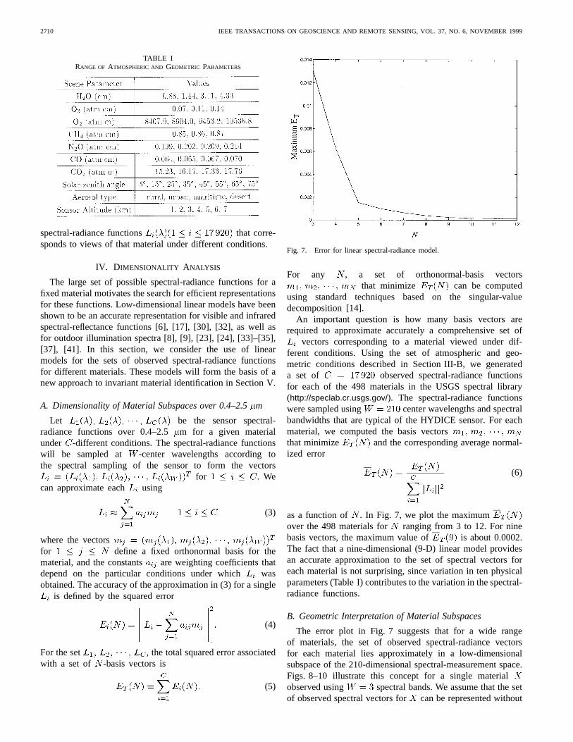
Fig. 7. Error for linear spectral-radiance model.

For any , a set of orthonormal-basis vectorsthat minimize can be computed

using standard techniques based on the singular-valuedecomposition [14].

An important question is how many basis vectors arerequired to approximate accurately a comprehensive set of

vectors corresponding to a material viewed under dif-ferent conditions. Using the set of atmospheric and geo-metric conditions described in Section III-B, we generateda set of observed spectral-radiance functionsfor each of the 498 materials in the USGS spectral library(http://speclab.cr.usgs.gov/). The spectral-radiance functionswere sampled using center wavelengths and spectralbandwidths that are typical of the HYDICE sensor. For eachmaterial, we computed the basis vectorsthat minimize and the corresponding average normal-ized error

(6)

as a function of . In Fig. 7, we plot the maximumover the 498 materials for ranging from 3 to 12. For ninebasis vectors, the maximum value of is about 0.0002.The fact that a nine-dimensional (9-D) linear model providesan accurate approximation to the set of spectral vectors foreach material is not surprising, since variation in ten physicalparameters (Table I) contributes to the variation in the spectral-radiance functions.

B. Geometric Interpretation of Material Subspaces

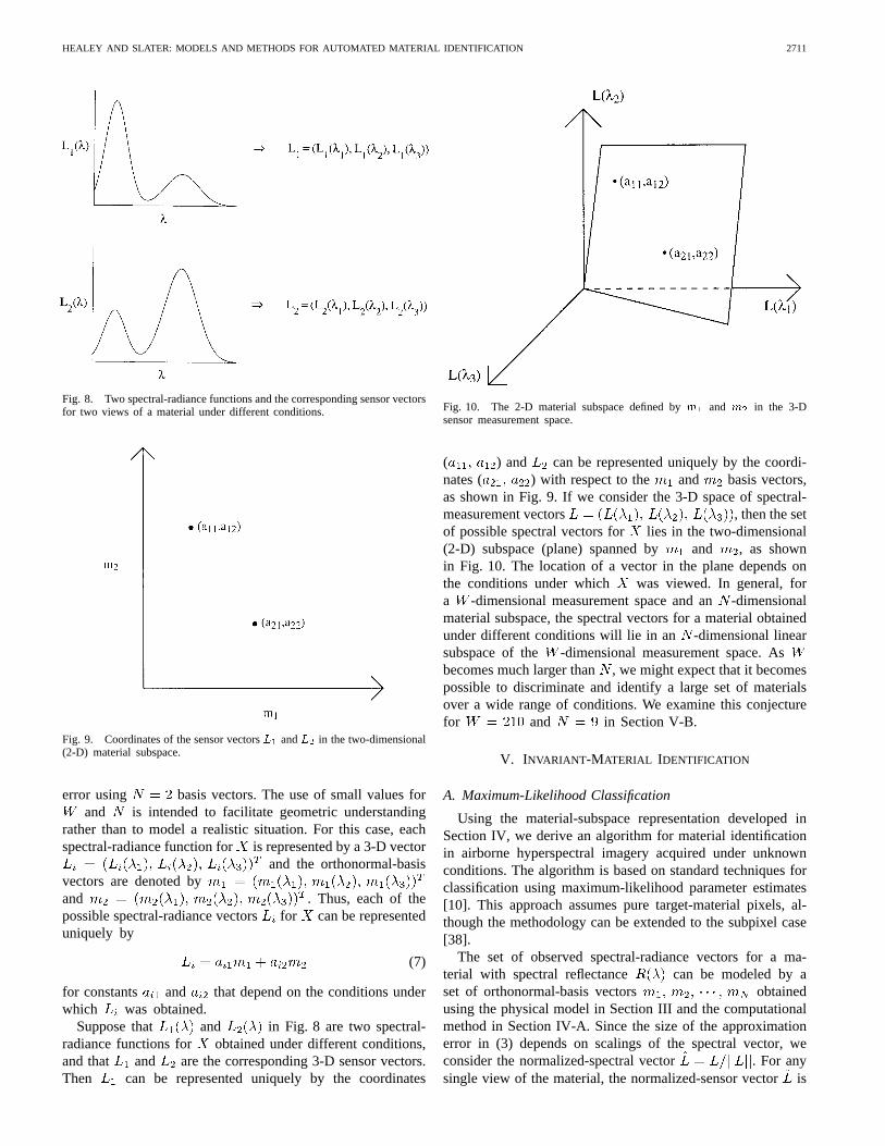
The error plot in Fig. 7 suggests that for a wide rangeof materials, the set of observed spectral-radiance vectorsfor each material lies approximately in a low-dimensionalsubspace of the 210-dimensional spectral-measurement space.Figs. 8–10 illustrate this concept for a single materialobserved using spectral bands. We assume that the setof observed spectral vectors for can be represented without


Fig. 8. Two spectral-radiance functions and the corresponding sensor vectorsfor two views of a material under different conditions.

Fig. 9. Coordinates of the sensor vectorsL1 andL2 in the two-dimensional(2-D) material subspace.

error using basis vectors. The use of small values forand is intended to facilitate geometric understanding

rather than to model a realistic situation. For this case, eachspectral-radiance function for is represented by a 3-D vector

and the orthonormal-basisvectors are denoted byand . Thus, each of thepossible spectral-radiance vectorsfor can be representeduniquely by

(7)

for constants and that depend on the conditions underwhich was obtained.

Suppose that and in Fig. 8 are two spectral-radiance functions for obtained under different conditions,and that and are the corresponding 3-D sensor vectors.Then can be represented uniquely by the coordinates

Fig. 10. The 2-D material subspace defined bym1 and m2 in the 3-Dsensor measurement space.

( ) and can be represented uniquely by the coordi-nates ( ) with respect to the and basis vectors,as shown in Fig. 9. If we consider the 3-D space of spectral-measurement vectors , then the setof possible spectral vectors for lies in the two-dimensional(2-D) subspace (plane) spanned by and , as shownin Fig. 10. The location of a vector in the plane depends onthe conditions under which was viewed. In general, fora -dimensional measurement space and an-dimensionalmaterial subspace, the spectral vectors for a material obtainedunder different conditions will lie in an -dimensional linearsubspace of the -dimensional measurement space. Asbecomes much larger than, we might expect that it becomespossible to discriminate and identify a large set of materialsover a wide range of conditions. We examine this conjecturefor and in Section V-B.

V. INVARIANT -MATERIAL IDENTIFICATION

A. Maximum-Likelihood Classification

Using the material-subspace representation developed inSection IV, we derive an algorithm for material identificationin airborne hyperspectral imagery acquired under unknownconditions. The algorithm is based on standard techniques forclassification using maximum-likelihood parameter estimates[10]. This approach assumes pure target-material pixels, al-though the methodology can be extended to the subpixel case[38].

The set of observed spectral-radiance vectors for a ma-terial with spectral reflectance can be modeled by aset of orthonormal-basis vectors obtainedusing the physical model in Section III and the computationalmethod in Section IV-A. Since the size of the approximationerror in (3) depends on scalings of the spectral vector, weconsider the normalized-spectral vector . For anysingle view of the material, the normalized-sensor vectoris


Fig. 11. Spectral-reflectance functions for target materials.

(a) (b)

Fig. 12. (a) ROC curves for sunlit target materials and(b) ROC curves forpartially shaded and concealed target materials.

described by

(8)

where the coefficients depend on the particular con-ditions under which the material is viewed and

is a residual vector. is chosenso that the approximation error in (3) is small and consequently

is modeled as a zero-mean Gaussian random vector withsmall covariance elements.

The likelihood of the sensor vector given a materialwith spectral reflectance and the parameter values

is

(9)

where is the covariance matrix of and

(10)

We note that the dependence of the likelihood on the spectralreflectance is expressed in the vectors.

If the covariance matrix is known, then maximum-likelihood estimates for the parameters canbe obtained by differentiating with respect to each

and setting the resulting expressions to zero. As aspecial case, if the elements of are independent with thesame variance (i.i.d. residuals), then the maximum likelihoodestimates for the parameters are given by

(11)

For this special case, the maximum-likelihood estimatesalso minimize the error

(12)

In general, the maximum likelihood estimates for theparameters can be substituted into (9) to obtain the likelihood

of observing the vector for amaterial with reflectance . This likelihood can be com-puted at each spatial location in the image and thresholdedfor material identification. In the case of i.i.d. residuals,


Fig. 13. Results for SAM algorithm on sunlit material samples.

Fig. 14. Results for invariant algorithm on sunlit material samples.

is a monotonically decreasing func-tion of

(13)

where the are computed using (11). For this case, the errorin (13) can be thresholded for material identification ratherthan the full likelihood .

B. Discriminability Analysis

Since the set of observed spectral vectors for a mate-rial lies in a low-dimensional subspace of the hyperspectral-measurement space, we might expect that there is little overlapamong the sets of vectors for different materials. We examined

this hypothesis by considering a representative spectral re-flectance for each of 100 materials in the USGS spectrallibrary. For each of the 100 materials, we generated 17 920spectral vectors, corresponding to the range of conditionspresented in Section III-B. Each vector consisted of 210spectral samples, corresponding to typical HYDICE centerwavelengths. The 17 920 spectral vectors for each materialwere used to compute a 9-D basis forthat material using the method described in Section IV-A.For any spectral vector , this allows computation of thelikelihood for each of the materials

. We proceeded to classify each of the1 792 000 vectors as an instance of the materialforwhich is the largest. The projectiondefined by (11) was used to estimate theparameters, and


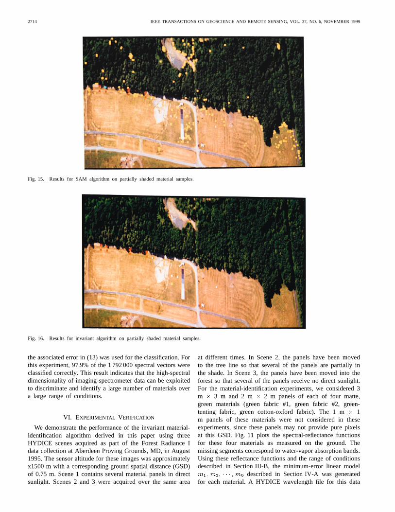
Fig. 15. Results for SAM algorithm on partially shaded material samples.

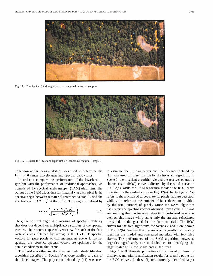
Fig. 16. Results for invariant algorithm on partially shaded material samples.

the associated error in (13) was used for the classification. Forthis experiment, 97.9% of the 1 792 000 spectral vectors wereclassified correctly. This result indicates that the high-spectraldimensionality of imaging-spectrometer data can be exploitedto discriminate and identify a large number of materials overa large range of conditions.

VI. EXPERIMENTAL VERIFICATION

We demonstrate the performance of the invariant material-identification algorithm derived in this paper using threeHYDICE scenes acquired as part of the Forest Radiance Idata collection at Aberdeen Proving Grounds, MD, in August1995. The sensor altitude for these images was approximatelyx1500 m with a corresponding ground spatial distance (GSD)of 0.75 m. Scene 1 contains several material panels in directsunlight. Scenes 2 and 3 were acquired over the same area

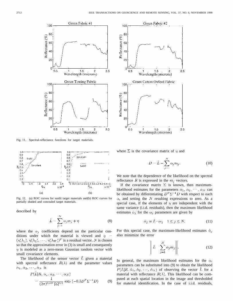
at different times. In Scene 2, the panels have been movedto the tree line so that several of the panels are partially inthe shade. In Scene 3, the panels have been moved into theforest so that several of the panels receive no direct sunlight.For the material-identification experiments, we considered 3m 3 m and 2 m 2 m panels of each of four matte,green materials (green fabric #1, green fabric #2, green-tenting fabric, green cotton-oxford fabric). The 1 m 1m panels of these materials were not considered in theseexperiments, since these panels may not provide pure pixelsat this GSD. Fig. 11 plots the spectral-reflectance functionsfor these four materials as measured on the ground. Themissing segments correspond to water-vapor absorption bands.Using these reflectance functions and the range of conditionsdescribed in Section III-B, the minimum-error linear model

described in Section IV-A was generatedfor each material. A HYDICE wavelength file for this data


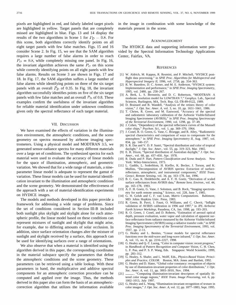
Fig. 17. Results for SAM algorithm on concealed material samples.

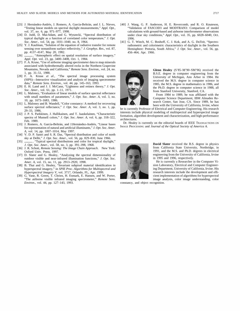
Fig. 18. Results for invariant algorithm on concealed material samples.

collection at this sensor altitude was used to determine thecenter wavelengths and spectral bandwidths.

In order to compare the performance of the invariant al-gorithm with the performance of traditional approaches, weconsidered the spectral angle mapper (SAM) algorithm. Theoutput of the SAM algorithm for materialat each pixel is thespectral angle between a material-reference vectorand thespectral vector at that pixel. This angle is defined by

(14)

Thus, the spectral angle is a measure of spectral similaritythat does not depend on multiplicative scalings of the spectralvectors. The reference spectral vector for each of the fourmaterials was obtained by averaging the HYDICE spectralvectors for pure pixels of that material in Scene 1. Conse-quently, the reference spectral vectors are optimized for thesunlit conditions in this scene.

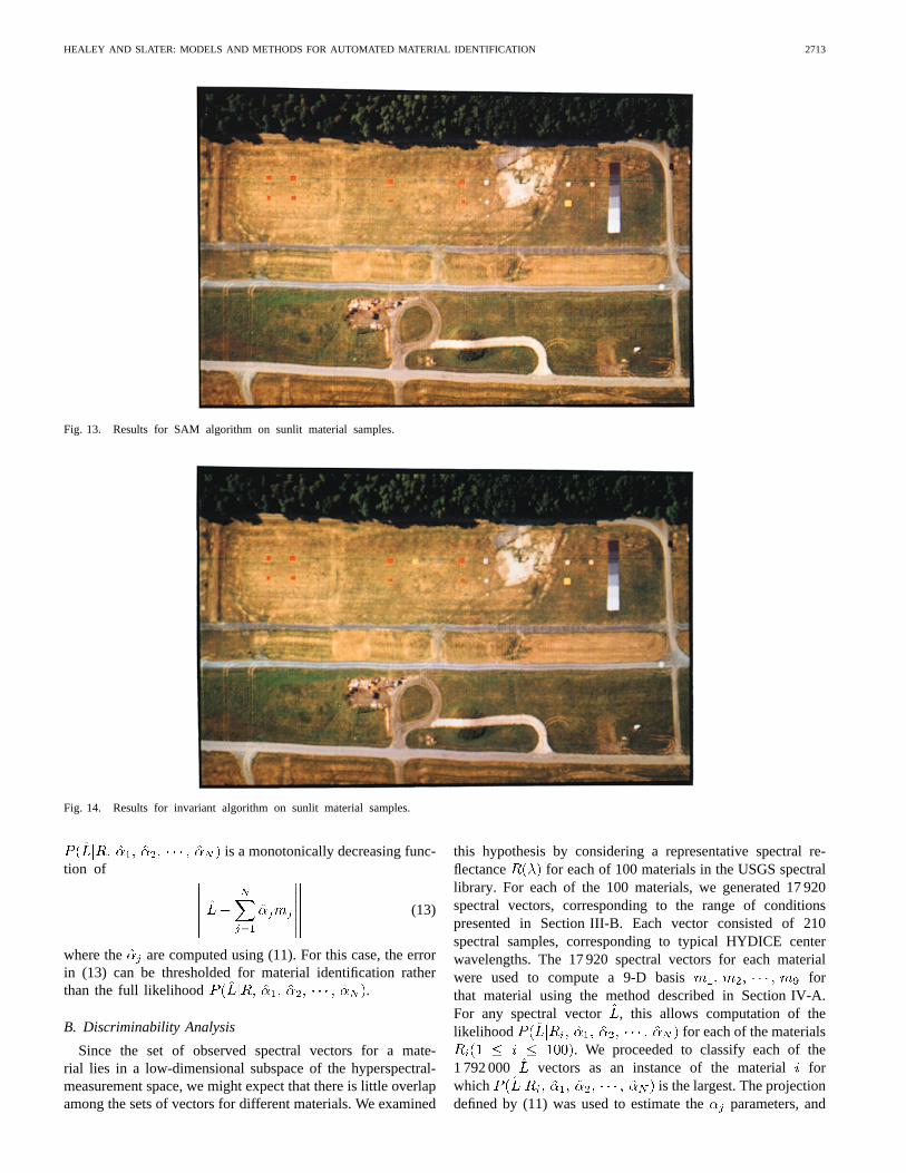
The SAM algorithm and the invariant material-identificationalgorithm described in Section V-A were applied to each ofthe three images. The projection defined by (11) was used

to estimate the parameters and the distance defined by(13) was used for classification by the invariant algorithm. InScene 1, the invariant algorithm yielded the receiver operatingcharacteristic (ROC) curve indicated by the solid curve inFig. 12(a), while the SAM algorithm yielded the ROC curveindicated by the dashed curve in Fig. 12(a). In the figure,refers to the fraction of target-material pixels that are detected,while refers to the number of false detections dividedby the total number of pixels. Since the SAM algorithmuses reference spectral vectors obtained from Scene 1, it wasencouraging that the invariant algorithm performed nearly aswell on this image while using only the spectral reflectancemeasured on the ground for the four materials. The ROCcurves for the two algorithms for Scenes 2 and 3 are shownin Fig. 12(b). We see that the invariant algorithm accuratelyidentifies the shaded and concealed materials with few falsealarms. The performance of the SAM algorithm, however,degrades significantly due to difficulties in identifying thetarget materials in the shade and in the trees.

Figs. 13–18 illustrate properties of the two algorithms bydisplaying material-identification results for specific points onthe ROC curves. In these figures, correctly identified target


pixels are highlighted in red, and falsely labeled target pixelsare highlighted in yellow. Target panels that are completelymissed are highlighted in blue. Figs. 13 and 14 display theresults of the two algorithms in Scene 1 for . Forthis scene, both algorithms correctly identify points on alleight target panels with few false matches. Figs. 15 and 16consider Scene 2. In Fig. 15, we see that the SAM algorithmrequires a large number of false alarms in order to reach

, while completely missing one panel. In Fig. 16,the invariant algorithm achieves the same on this scenewhile correctly identifying points on all eight panels with fewfalse alarms. Results on Scene 3 are shown in Figs. 17 and18. In Fig. 17, the SAM algorithm suffers a large number offalse alarms while identifying points on three of the six targetpanels with an overall of 0.35. In Fig. 18, the invariantalgorithm successfully identifies points on five of the six targetpanels with few false matches and an overall of 0.8. Theseexamples confirm the usefulness of the invariant algorithmfor reliable material identification under unknown conditionsgiven only the spectral reflectance of each target material.

VII. D ISCUSSION

We have examined the effects of variation in the illumina-tion environment, the atmospheric conditions, and the scenegeometry on spectra measured by airborne imaging spec-trometers. Using a physical model and MODTRAN 3.5, wegenerated sensor-radiance spectra for many different materialsover a large set of conditions. The synthesized spectra for eachmaterial were used to evaluate the accuracy of linear modelsfor the space of illumination, atmospheric, and geometricvariation. We showed that for a wide range of materials, a nine-parameter linear model is adequate to represent the gamut ofvariation. These linear models can be used for material identifi-cation invariant to the illumination and atmospheric conditionsand the scene geometry. We demonstrated the effectiveness ofthe approach with a set of material-identification experimentson HYDICE images.

The models and methods developed in this paper provide aframework for addressing a wide range of problems. Sincethe set of conditions considered in Section III-B includedboth sunlight plus skylight and skylight alone for each atmo-spheric profile, the linear model based on these conditions canrepresent mixtures of sunlight and skylight that might arise,for example, due to differing amounts of solar occlusion. Inaddition, since surface orientation changes alter the mixture ofsunlight and skylight received by a surface, this approach canbe used for identifying surfaces over a range of orientations.

We also observe that when a material is identified using thealgorithm derived in this paper, the corresponding coordinatesin the material subspace specify the parameters that definethe atmospheric conditions and the scene geometry. Theseparameters can be retrieved using a table lookup. With theseparameters in hand, the multiplicative and additive spectralcomponents for an atmospheric correction procedure can becomputed and applied over the image. Thus, the methodsderived in this paper also can form the basis of an atmospheric-correction algorithm that utilizes the information available

in the image in combination with some knowledge of thematerials present in the scene.

ACKNOWLEDGMENT

The HYDICE data and supporting information were pro-vided by the Spectral Information Technology ApplicationsCenter, Fairfax, VA.

REFERENCES

[1] W. Aldrich, M. Kappus, R. Resmini, and P. Mitchell, “HYDICE post-flight data processing,” inSPIE Proc. Algorithms for Multispectral andHyperspectral Imagery II, 1996, vol. 2758, pp. 354–363.

[2] R. W. Basedow, D. C. Armer, and M. E. Anderson, “HYDICE system:Implementation and performance,” inSPIE Proc. Imaging Spectrometry,1995, vol. 2480, pp. 258–267.

[3] A. Berk, L. S. Bernstein, and D. C. Robertson, “MODTRAN: Amoderate resolution model for LOWTRAN 7,” Geophys. Lab., SpectralSciences, Burlington, MA, Tech. Rep. GL-TR-89-0122, 1989.

[4] D. Brainard and B. Wandell, “Analysis of the retinex theory of colorvision,” J. Opt. Soc. Amer. A,vol. 3, no. 10, pp. 1651–1661, 1986.

[5] T. Chrien, R. Green, and M. Eastwood, “Accuracy of the spectraland radiometric laboratory calibration of the Airborne Visible/InfraredImaging Spectrometer (AVIRIS),” inSPIE Proc. Imaging Spectroscopyof the Terrestrial Environment, 1990, vol. 1298, pp. 37–49.

[6] J. Cohen, “Dependency of the spectral reflectance curves of the Munsellcolor chips,”Psychon. Sci., vol. 1, pp. 369–370, 1964.

[7] J. Conel, R. O. Green, G. Vane, C. Bruegge, and R. Alley, “Radiometricspectral characteristics and comparison of ways to compensate for theatmosphere,” inSPIE Proc. Imaging Spectrometry II, Aug. 1987, vol.834, pp. 140–157.

[8] S. R. Das and V. D. P. Sastri, “Spectral distribution and color of tropicaldaylight,” J. Opt. Soc. Amer., vol. 55, pp. 319–323, Mar. 1965.

[9] E. R. Dixon, “Spectral distribution of Australian daylight,”J. Opt. Soc.Amer., vol. 68, pp. 437–450, Apr. 1978.

[10] R. Duda and P. Hart,Pattern Classification and Scene Analysis. NewYork: Wiley-Interscience, 1973.

[11] L. Gaddis, L. Soderblom, H. Kieffer, K. Becker, J. Torson, and K.Mullins, “Decomposition of AVIRIS spectra: Extraction of surface-reflectance, atmospheric, and instrumental components,”IEEE Trans.Geosci. Remote Sensing, vol. 34, pp. 163–178, Jan. 1996.

[12] B. C. Gao, K. Heidebrecht, and A. F. H. Goetz, “Derivation of scaledsurface reflectances from AVIRIS data,”Remote Sens. Environ., vol. 44,pp. 165–178, 1993.

[13] A. F. H. Goetz, G. Vane, J. Solomon, and B. Rock, “Imaging spectrom-etry for earth remote sensing,”Science, vol. 228, June 7, 1985.

[14] G. H. Golub and C. F. van Loan,Matrix Computations. Baltimore,MD: Johns Hopkins Univ. Press, 1983.

[15] R. Green, B. Pavri, J. Faust, O. Williams, and C. Chovit, “Inflightvalidation of AVIRIS calibration in 1996 and 1997,” inJPL AirborneEarth Science Workshop, Pasadena, CA, Jan. 1998, pp. 193–203.

[16] R. O. Green, J. Conel, and D. Roberts, “Estimation of aerosol opticaldepth, pressure evaluation, water vapor and calculation of apparent sur-face reflectance from radiance measured by the Airborne Visible/infraredImaging Spectrometer (AVIRIS) using a radiative transfer code,” inSPIEProc. Imaging Spectrometry of the Terrestrial Environment, 1993, vol.1937, pp. 2–11.

[17] G. Healey and L. Benites, “Linear models for spectral reflectancefunctions over the mid-wave and long-wave infrared,”J. Opt. Soc. Amer.A, vol. 15, no. 8, pp. 2216–2227, 1998.

[18] G. Healey and Q.-T. Luong, “Color in computer vision: recent progress,”in Handbook of Pattern Recognition and Computer Vision, C. H. Chen,L. F. Pau, and P. S. P. Wang, Eds. Singapore: World Scientific, 1999,pp. 283–312.

[19] G. Healey, S. Shafer, and L. Wolff, Eds.,Physics-Based Vision: Princi-ples and Practice, COLOR. Boston, MA: Jones and Bartlett, 1992.

[20] G. Healey and D. Slater, “Global color constancy: recognition of objectsby use of illumination-invariant properties of color distributions,”J. Opt.Soc. Amer. A, vol. 11, pp. 3003–3010, Nov. 1994.

[21] , “Computing illumination-invariant descriptors of spatially fil-tered color image regions,”IEEE Trans. Image Processing, vol. 6, pp.1002–1013, July 1997.

[22] G. Healey and L. Wang, “Illumination-invariant recognition of texture incolor images,”J. Opt. Soc. Amer. A, vol. 12, pp. 1877–1883, Sept. 1995.


[23] J. Hernandez-Andrés, J. Romero, A. Garc´ıa-Beltran, and J. L. Nieves,“Testing linear models on spectral daylight measurements,”Appl. Opt.,vol. 37, no. 6, pp. 971–977, 1998.

[24] D. Judd, D. MacAdam, and G. Wyszecki, “Spectral distribution oftypical daylight as a function of correlated color temperature,”J. Opt.Soc. Amer., vol. 54, pp. 1031–1040, no. 8, 1964.

[25] Y. J. Kaufman, “Solution of the equation of radiative transfer for remotesensing over nonuniform surface reflectivity,”J. Geophys. Res., vol. 87,pp. 4137–4147, May 20, 1982.

[26] , “Atmospheric effect on spatial resolution of surface imagery,”Appl. Opt.vol. 23, pp. 3400–3408, Oct. 1, 1984.

[27] F. A. Kruse, “Use of airborne imaging spectrometer data to map mineralsassociated with hydrothermally altered rocks in the Northern GrapevineMountains, Nevada and California,”Remote Sens. Environ., vol. 24, no.1, pp. 31–51, 1988.

[28] F. A. Kruse et al., “The spectral image processing system(SIPS)—Interactive visualization and analysis of imaging spectrometerdata,” Remote Sens. Environ., vol. 44, pp. 145–163, 1993.

[29] E. H. Land and J. J. McCann, “Lightness and retinex theory,”J. Opt.Soc. Amer., vol. 61, pp. 1–11, 1971.

[30] L. Maloney, “Evaluation of linear models of surface spectral reflectancewith small numbers of parameters,”J. Opt. Soc. Amer. A, vol. 3, no.10, pp. 1673–1683, 1986.

[31] L. Maloney and B. Wandell, “Color constancy: A method for recoveringsurface spectral reflectance,”J. Opt. Soc. Amer. A, vol. 3, no. 1, pp.29–33, 1986.

[32] J. P. S. Parkkinen, J. Hallikainen, and T. Jaaskelainen, “Characteristicspectra of Munsell colors,”J. Opt. Soc. Amer. A, vol. 6, pp. 318–322,Feb. 1989.

[33] J. Romero, A. Garc´ıa-Beltran, and J.Hernández-Andrés, “Linear basesfor representation of natural and artificial illuminants,”J. Opt. Soc. Amer.A, vol. 14, pp. 1007–1014, May 1997.

[34] V. D. P. Sastri and S. R. Das, “Spectral distribution and color of northsky at Delhi,” J. Opt. Soc. Amer., vol. 56, pp. 829–830, June 1966.

[35] , “Typical spectral distributions and color for tropical daylight,”J. Opt. Soc. Amer., vol. 58, no. 3, pp. 391–398, 1968.

[36] J. R. Schott,Remote Sensing: The Image Chain Approach. New York:Oxford Univ. Press, 1997.

[37] D. Slater and G. Healey, “Analyzing the spectral dimensionality ofoutdoor visible and near-infrared illumination functions,”J. Opt. Soc.Amer. A, vol. 15, no. 11, pp. 2913–2920, 1998.

[38] B. Thai and G. Healey, “Invariant subpixel material identification inhyperspectral imagery,” inSPIE Proc. Algorithms for Multispectral andHyperspectral Imagery V, vol. 3717, Orlando, FL, Apr. 1999.

[39] G. Vane, R. Green, T. Chrien, H. Enmark, E. Hansen, and W. Porter,“The airborne visible infrared imaging spectrometer,”Remote Sens.Environ., vol. 44, pp. 127–143, 1993.

[40] J. Wang, G. P. Anderson, H. E. Revercomb, and R. O. Knuteson,“Validation of FASCOD3 and MODTRAN3: Comparison of modelcalculations with ground-based and airborne interferometer observationsunder clear sky conditions,”Appl. Opt., vol. 35, pp. 6028–6040, Oct.1996.

[41] G. T. Winch, M. C. Boshoff, C. J. Kok, and A. G. DuToit, “Spectro-radiometric and colorimetric characteristics of daylight in the SouthernHemisphere: Pretoria, South Africa,”J. Opt. Soc. Amer., vol. 56, pp.456–464, Apr. 1966.

Glenn Healey (S’85–M’90–SM’96) received theB.S.E. degree in computer engineering from theUniversity of Michigan, Ann Arbor in 1984. Hereceived the M.S. degree in computer science in1985, the M.S. degree in mathematics in 1986, andthe Ph.D. degree in computer science in 1988, allfrom Stanford University, Stanford, CA.

From 1984 to 1989, he was affiliated with theComputer Science Department, IBM Almaden Re-search Center, San Jose, CA. Since 1989, he hasbeen with the University of California, Irvine, where

he is currently Professor of Electrical and Computer Engineering. His researchinterests include physical modeling of multispectral and hyperspectral imageformation, algorithm development and characterization, and high-performancearchitectures.

Dr. Healey is currently on the editorial boards of IEEE TRANSACTIONS ON

IMAGE PROCESSINGand Journal of the Optical Society of America A.

David Slater received the B.S. degree in physicsfrom California State University, Northridge, in1991, and the M.S. and Ph.D. degrees in electricalengineering from the University of California, Irvinein 1995 and 1996, respectively.

He is currently a Researcher in the Computer Vi-sion Laboratory, Electrical and Computer Engineer-ing Department, University of California, Irvine. Hisresearch interests include the development and effi-cient implementation of algorithms for hyperspectralimage analysis, color image understanding, color

constancy, and object recognition.

models and methods for automated material identification

Documents