modellistica fisica per la protezione dell'ambiente
TRANSCRIPT

Alma Mater Studiorum - Universitá di Bologna
DOTTORATO DI RICERCA IN:
MODELLISTICA FISICA PER LA PROTEZIONE
DELL'AMBIENTE
Ciclo XXIV
Settore Concorsuale di affarenza: 08/A1
Settore scientifico - disciplinare di afferenza: ICAR/02
Lifelines in case of Natural Disaster Emergencies
Presentata da: Polyzoni Chrysanthi
Coordinatore Dottorato:
Prof. Rolando Rizzi
Relatore Dottorato:
Prof. Ezio Todini
Esame finale anno 2012

2

3
Executive Summary
Following a natural disaster, a lot of links of the road network may be unavailable or
interrupted. Certain segments such as bridges, tunnels or even normal streets may be
impossible for vehicles to circulate. This is a result of either the collapse of buildings
infrastructure failures, or road network flooding. This degradability creates both
inconvenience to local inhabitants and a huge barrier in rescue vehicles.
In order to handle such disasters, emergency areas are often individuated over the territory,
close to populated centres. In these areas, rescue services are located which respond with
resources and materials for population relief.
A method of automatic positioning of these centres in case of a flood or an earthquake is
presented. The positioning procedure consists of two distinct parts developed by the
research group of Prof Michael G. H. Bell of Imperial College, London, refined and applied to
real cases at the University of Bologna under the coordination of Prof Ezio Todini.
There are certain requirements that need to be observed such as the maximum number of
rescue points as well as the number of people involved. Initially, the candidate points are
decided according to the ones proposed by the local civil protection services. We then
calculate all possible routes from each candidate rescue point to all other points, generally
using the concept of the "hyperpath", namely a set of paths each one of which may be
optimal. The attributes of the road network are of fundamental importance, both for the
calculation of the ideal distance and eventual delays due to the event measured in travel
time units.
In a second phase, the distances are used to decide the optimum rescue point positions
using heuristics. This second part functions by "elimination". In the beginning, all points are
considered rescue centres. During every interaction we wish to delete one point and

4
calculate the impact it creates. In each case, we delete the point that creates less impact
until we reach the number of rescue centres we wish to keep.
The proposed technique was applied to the Aquila earthquake in 2009 in Italy, and the flood
in the Alessandria Region in 1994. All data was elaborated in the ESRI ArcGIS platform while
TeleAtlasTM road network data was also provided by ESRI Italia (dott Pietro Coffaro e dott
Fabrizio Pauri). A vast quantity of data was supplied by the Italian National Research Centre
- Hydrogeological section of Torino namely CNR - IRPI (Centro Nazionale delle Ricerche -
Instituto di Ricerca per la Protezione Idrogeologica del Consiglio) by dr Fabio Luino. The
National Institute of Geophysics and Vulcanology of Milan and Rome - Dr Stefano Salvi
(namely Istituto Nazionale di Geofisica e Vulcanologia di Milano INGV - Milan ) supported
the earthquake section of this research.

5
Executive Summary
In seguito ad un disastro naturale succede spesso che alcune parti della rete stradale siano
inutilizzabili o interrotte. Si può avere il danneggiamento di alcuni elementi come ponti o
gallerie oppure si può verificare che alcune strade risultino impercorribili a causa del crollo
dei palazzi vicini o del loro allagamento Il degradamento della rete stradale costituisce un
grande ostaccolo ai soccorsi.
Nella gestione di queste calamità si predispongono sul territorio aree di emergenza, in
prossimità o corrispondenza dei centri più popolati dei punti di soccorso dove vengono
localizzate risorse e materiali per il sostegno alle popolazioni colpite.
Si presenta un metodo di posizionamento automatico di questi centri di soccorso nel caso di
un terremoto o di un’alluvione. Il posizionamento avviene eseguendo due proccedure
sviluppate dal Gruppo di Ricerca del Prof Michael G. H. Bell dell’Imperial College di Londra e
perfezionate ed applicate a casi reali all’Università di Bologna sotto il coordinamento del
Prof. Ezio Todini.
Per posizionare in maniera ottimale i centri di soccorso devono essere rispettati alcuni
requisiti quali: il numero massimo di centri da posizionare e il numero massimo di abitanti
che un centro può soccorrere.
Inizialmente si decidono dei punti candidati all’interno della rete stradale (di solito proposti
dal dipartimento locale della Protezione Civile). Si calcolano tutti i possibili percorsi da ogni
punto (candidato per diventare punto di soccorso) verso tutti gli altri, utilizzando il concetto
dell’ "hyperpath" o ipercammino. I costi cosi calcolati rappresentano, in unità di tempo, i
tempi di percorrenza. Di fondamentale importanza sono i dati della rete stradale utilizzata.
Si utilizzano tutti gli attributi disponibili sia per valutare i tempi di percorrenza ideali sia per
stimare i possibili ritardi che sono dovuti al verificarsi dell’evento stesso.
In una seconda fase si usano i tempi individuati per decidere in modo euristico quali siano le
posizioni migliori dei punti di soccorso. Questa seconda parte della procedura funziona per
"eliminazione". All’inizio tutti i punti sono considerati come possibili punti di soccorso. Si
prova ad ogni iterazione ad eliminare un punto di soccorso e si calcola il costo di rimozione

6
Si elimina sempre il punto caratterizzato dal mnimo costo di eliminazione e si procede fino a
raggiungere un numero di punti di soccorso pari a quello desiderato.
La tecnica descritta è stata applicata alla Provincia dell’Aquila per il terremoto del 2009 e
alla zona di Alessandria per l’alluvione del 1994. Tutti i dati sono stati elaborati all’interno
della Platform ESRI ArcGIS e le reti stradali TeleAtlasTM usate sono state fornite da ESRI Italia
(dott Pietro Coffaro e dott Fabrizio Pauri). Una vasta quantita di dati è stata fornita dal CNR
- IRPI (Centro Nazionale delle Ricerche - Instituto di Ricerca per la Protezione Idrogeologica
del Consiglio) di Torino (dott Fabio Luino). Per la parte dei terremoti c’è stato il supporto
dell’Istituto Nazionale di Geofisica e Vulcanologia di Milano INGV - Milano e Roma (dott
Stefano Salvi).

7
Table of Contents
Chapter 1 ........................................................................................................................................ 15
Introduction ................................................................................................................................ 15
Global warming ........................................................................................................................... 16
Resilience and Vulnerability of transport networks ...................................................................... 17
Chapter 2 ........................................................................................................................................ 21
Emergency Management ............................................................................................................. 21
The Phases of emergency management ....................................................................................... 22
Mitigation ................................................................................................................................ 23
Preparedness ........................................................................................................................... 27
Response ................................................................................................................................. 28
Recovery .................................................................................................................................. 29
Chapter 3 ........................................................................................................................................ 31
The concept of the hyperpath...................................................................................................... 31
Introduction ................................................................................................................................ 31
Notation and Definitions ............................................................................................................. 32
Diksta algorithm .......................................................................................................................... 35
A star algorithm ........................................................................................................................... 35
Hyperpath ................................................................................................................................... 36
Chapter 4 ........................................................................................................................................ 49
Facility location concept .............................................................................................................. 49
Simple Plant location Problem ..................................................................................................... 53
Capacitated plant location problem ............................................................................................. 54
Location set covering problem ..................................................................................................... 55
Maximum covering location problems ......................................................................................... 55
Chapter 5 ........................................................................................................................................ 57
The mixed strategy ...................................................................................................................... 57
Description .................................................................................................................................. 57
Implementation steps.................................................................................................................. 58
Chapter 6 ........................................................................................................................................ 61
Flood responses .......................................................................................................................... 61
General Description ..................................................................................................................... 62

8
Cellular automata Flood Propagation Model ................................................................................ 67
Evacuation plans.......................................................................................................................... 71
Static pre-flood evacuation .......................................................................................................... 71
Static post-flood evacuation ........................................................................................................ 77
Dynamic, In motion evacuation ................................................................................................... 82
Case study Alessandria 2-6 November 1994................................................................................. 89
Position and hydrologic conditions .............................................................................................. 90
Flood dynamic ............................................................................................................................. 94
Built-up area vulnerability ........................................................................................................... 95
Simulation of the 2nd-6th November 1994 event into CA2D model ............................................. 97
Chapter 7 ........................................................................................................................................ 99
Earthquake responses ................................................................................................................. 99
Methodologies for seismic risk assessment.................................................................................. 99
The emergency plan (rescue centre location in uncertain degraded road networks) .................. 100
Post earthquake uncertainties ................................................................................................... 101
Fault displacement ................................................................................................................ 102
Earthquake Induced Landslides .............................................................................................. 103
Liquefaction ........................................................................................................................... 103
Vulnerable components ......................................................................................................... 104
L’Aquila earthquake 2008 .......................................................................................................... 104
Chapter 8 ...................................................................................................................................... 113
Discussion ..................................................................................................................................... 113
References .................................................................................................................................... 117
APENDIX ........................................................................................................................................ 123
Introduction .............................................................................................................................. 123
ESRI support .............................................................................................................................. 123
Data collection .......................................................................................................................... 123
Code implementation ................................................................................................................ 132
Flood and earthquake data implementation .............................................................................. 132
Rescue Centres - L'Aquila earthquake 6th May 2009 .................................................................. 133

9
Acknowledgements
I would like to express my gratitude to my tutor Prof Ezio Todini, for his support and
guidance. Furthermore I would like to thank Dr Francesco Dottori and the rest of my
colleagues at the University of Bologna. Many thanks to prof Michael G. H. Bell and Dr
Achille Fonzone from the Imperial College of London for their continuous guidance during
the time I spent abroad.
A continuous support was provided from Dr Fabio Luino from the Italian Research Council,
Torino chair. Additionally I would like to thank ESRI Italia (Eng. Pietro Coffaro and Dr Fabrizio
Pauri) who provided both software and data licenses, for the needs of this research.
Further, I would like to thank the National Institute of Geophysics and Vulcanology, Dr. Vera
Pessina (Milan section) and Dr Stefano Salvi (Rome section) for their assistance and data
contribution.
A big thank you goes to Dr Kostas Prodromou for taking the time to read this thesis and
provide me with extremely useful comments.

10

11
List of Figures
Figure 1-1 Global warming for flooding ............................................................................................ 17
Figure 3-1 illustrated in blue the links out of node i Ai
and in red the links into node i Ai
........ 37
Figure 6-1 TeleAtlasTM sample map - representation of a road network. The nodes are the junctions
and the links are the streets of the transport network .................................................................... 62
Figure 6-2 (a) Sample of a street map (TeleAtlas streetmap), a representation of a road network.... 66
Figure 6-3 (b) ) Terminal points: purple points represent terminal point locations ........................... 66
Figure 6-4 (c) Population centers: green points represent population centre locations .................... 67
Figure 6-5 Input data for the proposed system, (a) Sample of a street map (TeleAtlas streetmap), a
representation of a road network, (b) Terminal points: purple points represent terminal point
locations, (c) Population centers: green points represent population centre locations ..................... 67
Figure 6-6 (a)Demonstration of all available paths from each population centre to terminal point No
"1"................................................................................................................................................... 72
Figure 6-7 (b) Demonstration of all available paths from each population centre to terminal point No
"2"................................................................................................................................................... 72
Figure 6-8 (c) Demonstration of all available paths from each population centre to terminal point No
"3"................................................................................................................................................... 73
Figure 6-9 (d) Demonstration of all available paths from each population centre to terminal point No
"4", .................................................................................................................................................. 73
Figure 6-10 (e) Demonstration of all available paths from each population centre to terminal point
No "5" ............................................................................................................................................. 74
Figure 6-11 (f) ) Demonstration of all available paths from each population centre to terminal point
No "6". ............................................................................................................................................ 74
Figure 6-12 Static pre flood evacuation emergency plan . There are not blocked streets due to the
emergency because the alarm was announced on time before the evacuation (time local civil
protection decides). (a) Demonstration of all available paths from each population centre to terminal
point No "1", (b) Demonstration of all available paths from each population centre to terminal point
No "2", (c) Demonstration of all available paths from each population centre to terminal point No
"3", (d) Demonstration of all available paths from each population centre to terminal point No "4",
(e) Demonstration of all available paths from each population centre to terminal point No "5", (f ... 74
Figure 6-13 Hyperpath costs, evacuation before the “flood wave" - Static Version -Time in seconds 75
Figure 6-14 Assignment of population centres to their related terminal points. ............................... 76
Figure 6-15 (a) Demonstration of all available paths from each population centre to terminal point
No "1" ............................................................................................................................................. 77
Figure 6-16 (b) Demonstration of all available paths from each population centre to terminal point
No "2" ............................................................................................................................................. 78
Figure 6-17 (c) Demonstration of all available paths from each population centre to terminal point
No "3" ............................................................................................................................................. 78
Figure 6-18 (d) Demonstration of all available paths from each population centre to terminal point
No "4" ............................................................................................................................................. 79
Figure 6-19 (e) Demonstration of all available paths from each population centre to terminal point
No "5" ............................................................................................................................................. 79

12
Figure 6-20 (f) Demonstration of all available paths from each population centre to terminal point No
"6"................................................................................................................................................... 80
Figure 6-21 Static post flood emergency evacuation plan(a) Demonstration of all available paths from
each population centre to terminal point No "1", (b) Demonstration of all available paths from each
population centre to terminal point No "2", (c) Demonstration of all available paths from each
population centre to terminal point No "3", (d) Demonstration of all available paths from each
population centre to terminal point No "4", (e) Demonstration of all available paths from each
population centre to terminal point No "5", (f)Demonstration of all available paths from each
population centre to terminal point No "6". .................................................................................... 80
Figure 6-22 Evacuation after the "flood alarm"-Static Version -Time in seconds ............................... 81
Figure 6-23 Assignment of population centres to the optimum terminal points after the "flood
wave"-Static Version ....................................................................................................................... 81
Figure 6-24 (a) two hours after the beginning of the flood ............................................................... 82
Figure 6-25 (b) four hours after the beginning of the flood .............................................................. 83
Figure 6-26 (c) six hours after the beginning of the flood ................................................................. 83
Figure 6-27 (d)eight hours after the begining of the flood ................................................................ 84
Figure 6-28 CA2D flood plain model: CA2D model interpretation two hours after the beginning of the
flood (a), CA2D model interpretation four hours after the beginning of the flood (b), CA2D model
interpretation six hours after the beginning of the flood (c), CA2D model interpretation eight hours
after the beginning of the flood (d) .................................................................................................. 84
Figure 6-29 Flood evolution of the "Alessandria 1994" event according to CA2D flood propagation
model .............................................................................................................................................. 85
Figure 6-30 Travel times calculated from each population centre to each terminal point respectively.
........................................................................................................................................................ 85
Figure 6-31 Assignment of population centres to the optimum terminal points according to the
dynamic solution with fixed da values .............................................................................................. 86
Figure 6-32 (a) , after four hours from the arrival of the flood wave................................................. 88
Figure 6-33 (b) , after four hours from the arrival of the flood wave ................................................ 88
Figure 6-34 (c) , after four hours from the arrival of the flood wave ................................................. 89
Figure 6-35 (d) , after four hours from the arrival of the flood wave ................................................ 89
Figure 6-36 Assignment of terminal points to their related population centres the first two hours
from the arrival of the flood wave (a), after four hours from the arrival of the flood wave (b), after six
hours from the arrival of the flood wave, (c) after eight hours from the arrival of the flood wave .... 89
Figure 6-37 Position of Tanaro River basin ....................................................................................... 91
Figure 6-38 Position of case study.................................................................................................... 92
Figure 6-39 Position of hydrometric stations in 1994. Source EVENTI ALLUVIONALI IN PIEMONTE
(Torino 1998)................................................................................................................................... 92
Figure 6-40 Perceptions of hydrometric stations of Tanaro basin during 2-6 of November 1994.
Source EVENTI ALLUVIONALI IN PIEMONTE (Torino 1998) ............................................................... 93
Figure 6-41 Infrastructure failure during the catastrophic phase of the flood (third phase 6th of
November 1994 13:00-14:30 GMT+1 ) ............................................................................................ 95
Figure 6-42 Urbanization of the city of Alessandria (a) 1851, (b) 1875, (c) 1933, (d) 1991, Luino. F. et
al (1994) .......................................................................................................................................... 96

13
Figure 7-1 Macroseismic intensity of the earthquake occurred at the Aquila Region on the 6th of
April 2009 - Official data INGV ....................................................................................................... 105
Figure 7-2 Hyperpath example from node 9................................................................................... 106
Figure 7-3 Hyperpath example from node 56 ................................................................................. 106
Figure 7-4 Hyperpath example from node 62 ................................................................................. 107
Figure 7-5 Hyperpath example from node 63 ................................................................................. 107
Figure 7-6 Hyperpath example from node 63 ................................................................................. 108
Figure 7-7 Hyperpath example from node 64 ................................................................................. 108
Figure 7-8 Hyperpath example from node 66 ................................................................................. 109
Figure 7-9 Rescue Centres Decided by the Civil Protection ............................................................. 110
Figure 7-10 Rescue Centes Proposed by the model ........................................................................ 111
Figure 0-1 Base maps Provided by Dr Fabio Luino CNR di Torino .................................................... 125
Figure 0-2 Base maps Provided by Dr Fabio Luino CNR di Torino .................................................... 126
Figure 0-3 Orthophoto provided by the CNR of Torino (Dr Fabio Luino) ......................................... 127
Figure 0-4 Orthophoto provided by thr CNR di Torino (Dr Fabio Luino) .......................................... 128
Figure 0-5 Alessandria Road Network - MultinetTM Data ................................................................ 130
Figure 0-6 L'Aquila Network Multinet Data .................................................................................... 131
Figure 0-7 Rescue Centres along L'Aquila Municipality Network .................................................... 134

14
15
Chapter 1
Introduction
Natural and technological disasters (International Federation of Red Cross and Red Crescent
Societies, 2011) keep on imposing very high tolls on human kind (Centre for Research on the
Epidemiology of Disasters, 2011). In 2010 385 natural disasters have been recorded, causing
more than 297,000 fatalities and US$ 123.9 billion of damages. In 2010 an earthquake in
Haiti (12 January) resulted in 222,641 deaths; floods and landslides in China (May to August)
affected more than 145 million people; an earthquake of magnitude 8.8 on the moment
scale (27 February) cost Chile US$ 30 billion (Guha-Sapir et al., 2011).
The individuation of natural hazard prone areas, permits a comprehensive defend actions
organization from the part of civil protection department (both national and local). Such
natural disasters may include geological, hydro geological, geomorphologic, geophysical, etc
interest.
Natural hazard phenomena manifest periodical impact. The goal is to capture their rhythm
although intensity may vary from time to time. Furthermore natural hazards lead to actual
disasters only when the natural event impacts on a vulnerable environment. Vulnerability

16
can be reduced by the adoption of emergency management measures before, during and
after the occurrence of adverse events. Comprehensive Emergency Management considers
four stages in dealing with adverse events: mitigation, preparedness, response, and
recovery (Green III, 2002). Systematic reviews of research on optimization of disaster
management activities are provided by Altay and Green III (2006) and Caunhye et al (in
press). The latter classifies the research on the logistics of humanitarian relief chains –
crucial in the preparedness and response phases – into two categories: 1) facility location; 2)
relief distribution and casualty transportation.
We present a method to locate repositories of resources for humanitarian relief chains
(referred to as “terminal points” in the following) to face emergencies generated by natural
disasters such as floods. Both the demand points (referred to as “population centres”) and
the candidate locations for terminal points coincide with the nodes of a transport network
which can be degraded by the disaster. It is assumed possible to estimate for each link the
maximum additional cost (or delay) caused by the damages generated by the disaster. The
problem is formulated as a two stage optimization problem: The primary problem is a
capacitated p-median problem in which the location of p rescue centres is sought which
minimizes the overall weighted best-worst cost between rescue centres and population
centres
Global warming
Global average temperature rises are evident in most people's experience. Rise in the
average temperature of Earth's atmosphere and oceans is commonly known as Global
warming. Earth’s surface average temperature increased almost 0.8°C over the past 100
years, while 0.6 °C of this warming occurred over the last three decades. This phenomenon
is very likely caused by the emission of greenhouse gases from human activities (e.s.
deforestation and burning fossil fuels). Actually, 97–98% of climate researches support the
outcomes of the Intergovernmental Panel on Climate Change, on the tenets of
Anthropogenic Climate Change (ACC) (William R. L. Anderegg, James W. Prall, Jacob Harold,
Stephen H. Schneider, 2010). However there are a few climate scientists sceptic about this
issue (Arrhenius, 1896) (Page, 2007) (Berkeley Earth Team, 2011) (Kai-Uwe Eichmann, 2011).

17
However it is very important that 97% of active climate researchers agree with the
Intergovernmental Panel on Climate Change executive summary. Should we note that
Global climate is a very complex system, processes are diverse and cover many fields.
There is no doubt that humans are altering the climate, but the implications for regional
weather are less clear. No computer simulations exist in order to give a conclusion about a
given snowstorm or flood due to global warming. But with a combination of climate models,
weather observations and a good dose of probability theory, scientists may be able to
determine how climate warming changes the odds. Nonetheless, this poses significant risks
for a range of human and natural systems. And these emissions continue to increase, which
will result in further change and greater risks.
An increase in global temperature causes sea levels rise and changes the amount and
pattern of precipitation. The insurance industry has long worried about increased losses
resulting from more extreme weather. It is not yet certain, if put the blame on climate
change, may give the answer. Indeed it may take long time to prove (Schiermeier, 2011) but
somehow it is the case to take this matter into consideration when it comes to talk about
flooding issues.
Figure 1-1 Global warming for flooding
Resilience and Vulnerability of transport networks
Investigation of short to medium term operational vulnerability and resilience of transport
networks analysis is commonly accepted as a very important step to reduce the catastrophic
impact of natural disasters. This may also include identify longer term network adaptation
issues raised by climate change if this is not addressed.

18
We can reach somehow the concept of vulnerability through bibliography of the last ten
years. Berdica (2002) presents a detailed terminology for vulnerability. Vulnerability should
focus on the impacts of the different threats to the network and not on the threats
themselves. However a generally recognized definition for resilience is not recognised. Yet
there have been identified some key properties that have been used to gauge the resilience
of a transport network by Murray-Tuite, P.M. (2007) and reported by Christopher Mason.,
2010
Redundancy. In the transport network there are some similar one to each other
components, from the functionality point of view that can serve the same target and
therefore the system does not fail when one of its components fails (there may be
available more than one paths to go from one place to another).
Diversity. There may be different functional components so as to be protected
against various threats (there must be different travel modes to go from one place to
another).
Environmental Efficiency. For a sustainable transport system, capacity constraints
may produce less impact to itself due to environmental reasons.
Autonomy. Different components of the transport system should be able to operate
independently. In such way, one components failure, would not cause the failure of
others. (Eventual efficiency of the transport system be in case of electricity power
cut).
Strength. The robustness of a transport systems against an incident (the
"magnitude" of a natural hazard the system may afford).
Adaptability. The flexibility of the transport system to adapt to changes. This may
include the capacity to change through different experiences (different traffic
conditions in the same area).
Collaboration. Different components of the transport system share the same
information or resources are shared (adaption of the same plans in case of an
emergency and the ability or responsibility for different system operators to
communicate).
Mobility. Users of the transport system should be able to arrive to the desired
destination in an acceptable time.

19
Safety. The transport system should be robust enough so as protect travellers in case
of an unexpected hazard and not expose them to additional risks.
Recovery. The transport system should be able to quickly recover up to a reasonable
level after the occurrence of a routine incident.

20

21
Chapter 2
Emergency Management
Emergency management is the generic term of a multidisciplinary field. It generates
strategies and processes used to protect critical assets of an organization from hazard
risks that can cause events like disasters or catastrophes. It is also responsible to ensure the
continuance of an organization within their planned lifetime. Comprehensive emergency
management can be defined as the preparation for and the carrying out of all emergency functions
whether natural, technological, or human caused. It includes more than one components in order to
be prepared for each hazard considering all hazards, its phases and its impacts.
Catastrophes, Emergencies or Disasters, are not linear fields; they are discrete issues
causing different problems that require distinct strategies of response. These differences
need specific planning and management activities for their relevant crisis groups both
quantitatively and qualitatively (Quarantelli, 2000).
Emergency Management is considered strategic and not tactical process. As a result it is
very often treated by the highest level management in an organization. It has no direct

22
power generally, but corporate as a coordinating or advisory function to ensure that all
elements of an organization are emphasised on the desired target. Effective Emergency
Management is firstly based on the integration of emergency plans at all levels of a certain
organization. After that is very important to ensure that each level of the specific
organization is capable to apply the decisions taken under crisis state, be responsible
enough to manage the emergency, receive additional resources and assistance from the
upper levels when needed.
Last but not least, Emergency Management has a certain hierarchy led by a specialist
normally called Emergency Manager. He is in charge of creating the framework within
which communities reduce vulnerability to hazards and cope with disasters.
In summary, Emergency management has a certain definition, Vision, Mission and Principles
(IAEM, 2007) . Emergency management is the managerial function in charged to create the
lines within which communities reduce vulnerability to hazards and cope with disasters. It's
vision is to promote safer communities with the capacity to cope with hazards and disasters.
Its mission is to protect the community by coordinating all necessary activities capable to
mitigate against, prepare for, respond to, and recover from threatened or actual natural
disasters, acts of terrorism, or other man-made disasters.
A successful Emergency manager must be Comprehensive, Progressive, Risk-Driven,
Integrated, Collaborative, Coordinated, Flexible and Professional based on, training,
experience, ethical practice, public stewardship and continuous improvement (IAEM, 2007).
The Phases of emergency management
Comprehensive Emergency Management includes four distinct phases based on local and
economical conditions. Namely these four phase s are Mitigation, Preparedness, Response and
Recovery. All four phases highly depend on the long term work on infrastructure, public awareness
and even legal and justice issues.

23
In United states Emergency Management is mainly driven since 1979 by the Federal Emergency
Management Agency (FEMA). FEMA is a government institution that deals with all phases four
phases of natural and technological disasters as well as terrorist actions etc
In Europe natural and technological disasters are organised by the Civil Protection Departments
different for every country. Organization and functional standards vary from country to country
since there does not exist a main driven organization to generally provide the guidelines for
mitigation, preparedness, response and recovery.
Italian Civil protection is one of the most effective organizations in Europe that cover all four
phases of Natural disasters in the Italian territory.
Mitigation
The first phase of emergency management analyzed is mitigation which in general deals
with the prevention of hazards before these, are developed into disasters. This phase efforts
to reduce life and property loss by preventing the impact of disasters. There are plenty of
mitigation activities which achieve to calculate the risk over certain natural or man-made
disasters and provide a methodologies to reduce it. Such information can be provided by
Risk analysis foundations and flood insurance that protects financial investment. Mitigation
analysis phase differs from the other phases of emergency management in the sense that it
mainly focuses on long term studies for reducing or eliminating risk. Mitigation strategies
can then be implemented as part of the recovery phase, if applicable following a disaster.
Mitigation measurements may apply either structural or non structural units. Technological
solutions are generally used for structural measurements when we have to deal with flood
levees or building retrofitting for earthquakes. Non structural measurements instead, often
deal with legislation, land-use planning ( for example create non essential land such as parks
to be used as floodplains) and insurance.
Many times there has been stated that the most cost-efficient method for reducing the
effect of hazards is through mitigation. However this is not always the most suitable
solution. Strategies included in this phase include regulations regarding evacuation plans,
sanctions against those who refuse to apply decided regulations (for example mandatory

24
evacuations), and communication of risks to the public. It is also possible that some
structural mitigation measurements may harm the ecosystem.
A precursor to mitigation is the identification of risks. Physical risk assessment refers to
identifying and evaluating hazards. The hazard-specific risk (Rh) combines a hazard's
probability and effects.
Determination of Hydrogeological Risk and Loss
In analytical terms, hydro geological risk is expressed in the following equation. This
equation connects hazard, vulnerability to the exposed value (the value exposed to the risk):
Risk = hazard x vulnerability x exposed value
"Hazard" term expresses the probability that in a certain zone is verified a damaging event
of a certain intensity during a certain period of time (this period of time is referred to as
"return time"). Hazard therefore function of the frequency of the event. In certain cases
when we mainly deal with floods it is possible to calculate an acceptable approximation of
the return period. For other hydro geological risks, such as certain types of landslides, such
estimation is way more difficult to obtain.
Vulnerability instead, indicates the attitude of a certain "environmental component" (such
as human population, buildings infrastructures, services, etc) to support the effects in an
intensity bases, due to the event itself. Vulnerability expresses the level of loss of a certain
element or a series of elements as a result of the verification of a stated "magnitude"
expressed in a scale from zero (no damage) to one (absolute destruction). The exposed
value (or exposition) indicates the element that has to support the event. The event can be
expressed either form the presence of human lives, or from the value of natural and
economical resources exposed to a certain danger.
The product Vulnerability x Exposed value thus indicates the consequences deriving from
humans in terms both of human loss and damages in building and in general infrastructures
or the producing system. The risk expresses therefore the expected number of human loss,
human injuries, property loss, economical activity loss natural recourses loss due to

25
particular harmful event; in other words risk is the product of the probability of occurrence
of a certain event with the event's dimension itself.

26
Determination of Seismic Risk and Loss
For the occurrence of an earthquake the standard definition of risk is the same. However
Risk and loss are described separately. Seismic risk is thus the probability or likelihood of
damage and consequent loss to a given element at risk, over a specified period of time.
It is important to note again the distinction between risk and vulnerability. Risk combines
the usual losses from every level of hazard severity, taking also into account their
occurrence and probability, while an element's vulnerability is usually stated for a given
hazard severity level (Coburn et al. 1994).
Loss is defined as the human or and economical results of an individual damage, along with
injuries or deaths, the costs of repair, or loss of profits. The distinction between risk and loss
many times is not clear and always generated based on their definition; these two terms are
very often used equally. Taking into consideration that the standard definition of risk is a
probability or likelihood of loss (from zero to one) it may be more appropriate to express
risk as
Risk = Hazard ×Vulnerability
On the other hand loss depends on the value of the exposure at risk, given by
Loss = Hazard×Vulnerability×Exposure
As a result, while seismic hazard is genuinely a product of natural processes, seismic risk and
loss depend on the vulnerability and societal exposure in terms of the infrastructure
environment, human population, and value of processes.

27
Preparedness
The term Preparedness deals with the way we change our behaviour in order to limit a
disaster's impact to ether individuals or organizations. This includes an eterne cycle of,
evaluating, , monitoring, planning, training, managing, equipping, exercising, creating and
improving actions to guarantee efficient organization and the connection of all available
capabilities of concerned organizations to either protect or create resources against natural
or manmade disasters but even terrorist actions or other causalities that may create human
and natural inconvenience.
An emergency manager, for the preparedness phase, needs to focus on the development of
emergency plans. During effective Risk management, there are counted individual risks as
well as are organised specified activities. In such way are created the necessary capabilities,
needed to implement such plans. Common preparedness measures include:
Communication plans with clear process and terminology.
Efficient maintenance of emergency services and continuous training and updating
of qualified personnel, including mass human resources such as community
emergency response teams.
Continuous tests and development of early warning methods. This would include
determination of emergency shelters (such as rescue centres or terminal points) and
efficient evacuation plans.
Relief supply chain which includes inventory of the target zone, streamline, food and
medicine supplies and equipment.
Take advantage of and gather together specific organizations, trained volunteers and
local communities. Emergency operator professionals are immediately overpowered
after mass emergencies so responsible trained and organized volunteers are very
valuable. There exist organizations that provide spontaneous trained volunteers
such as the "Red Cross" and "Community Emergency Response Teams". Red Cross's
emergency management system has received high ratings all over the world.
Last but not least, another key issue of the preparedness phase of emergency
management is "casualty prediction", which is the study of the loss we can expect
due to a certain event in terms of deaths or injuries. "Casualty prediction" may form

28
an opinion to planners about the required resources needed so as to respond to a
particular sort of event.
As long as planning phase lasts, Emergency Managers should be both flexible, and all
encompassing. They should carefully recognize both exposure and risks the of the regions
they are responsible for, and be eligible to employ unusual or unconventional systems of
aid. Depending on the category of the emergency service that can be applied to a region,
municipality or even a certain private sector, emergency services can immediately be
consumed and overcharged. Mutual aide compromises between nongovernmental
organizations, which offer desired resources, and rescue groups is important to be
distinguished in the first stages of planning process and applied with uniformity.
Response
In the response phase we can individuate the mobilisation of all available emergency
services needed which would be naturally pat of the first services to respond at the disaster
zone. This is possible to include emergency vehicles of fire-fighters, ambulances or even
police and army forces. Civilian emergency resources apply to the first wave, or core
emergency services. In the case where military operations are needed a Disaster Relief
Operation is conducted. When this occurs it is very often the case where a non combatant
evacuation may follow. Several secondary emergency services may participate such as
specialist rescue teams.
When an emergency plan is efficiently structured, the coordination of rescue teams is less
hard to handle. There are times where search and rescue teams (Search And Rescue -SAR
teams) have to react at a very early stage. This depends on injuries supported by the victims,
weather conditions, victims possibility to escape from the disaster area or access to air and
water. The majority of victims affected by a disaster may pass away within 72 hours within
the impact if not helped.
From the organization point of view, a comprehensive response to a significant disaster
(which could be ether a natural disaster -man-made- or a terrorist ) is mainly based on the

29
existing processes and systems of the actual emergency management structure. This may
include a Response Plan and the Incident Command System.
Both agility and discipline are needed in responding to a disaster. An efficient leadership
also needed in order to onboard and built a quick coordination and solve problems as they
grow over the first responses. The suitable leader, together with the responsible and trained
team have to work together and implement an already robust emergency plan for the
specific needs of each disaster.
Recovery
The goal of the recovery phase is to rebuilt, reconstruct and renovate the area affected by
the disaster to its prior condition. There are certain directions people should follow in order
to facilitate recovery. This may include health and safety guidelines, maybe clean a damaged
home and rebuilt it safer for the future, take certain precautions while going back home or
even ask for assistance. More generally re-employment, and repair of all essential
infrastructure. Other human aspects after a disaster is cope with the emotional effects of a
disaster, help children or others cope with such feelings over recovery.
Main efforts should focus to build a better and more robust environment aiming to reduce
the pre-disaster risks organically in the community and infrastructure. A very significant
aspect of effective recovery efforts is taking advantage of the instructions given and maybe
the opportunity implement discrete measures and keep in mind that disasters (especially
natural disasters) have a period of return and thus it is very likely to happen again. This is
why measurements need to be taken as soon as possible in order to avoid more severe
consequences. Citizens of the affected area are more likely to accept more changes when a
recent disaster is in fresh memory.
There are three general phases that take place during recovery after a natural disaster. Both
actions and timing vary respect to the severity and the nature of the disaster. The first phase
deals with direct actions taken to reduce life-threaten hazards and prepare short-term
repairs to critical lifelines. The second phase consists of the preparation of social needs
during the reconstruction of damaged infrastructure. This phase may last several weeks,
months or even a couple of years. The third phase consists of implementing all

30
reconstructions of damaged buildings and other facilities or infrastructure as well as the
continuation of normal financial and social life in the community. This may also include a
review of pre-disaster status. This third phase may last way long tame, may in fact continue
for some years.

31
Chapter 3
The concept of the hyperpath
Introduction
The problem of searching a route in a network that consists of links and nodes is mostly
encountered by transport engineering. However it is very often computer sciences and (or)
operational research that deals with searching problems and thus problems such as
minimization, maximization or capacity of a denoted value. The network, or in other words
the directed graph, represents in our case a street map where the links are different road
elements (roads, bridges, tunnels) and the nodes are the junctions.
There has been proposed a lot of network searching techniques in the past and thus a lot of
research to form a search tree, beginning from a certain origin and arriving to the desired
destination. There are algorithms seeking to find the optimal route in a certain network
(with respect to the criterion to be optimized) and others that guarantee to find any
possible available solution. The first ones are called optimal and the second ones heuristic.
The concept of the hyperpath derives initially from a specific field of transport engineering
known as transit assignment (Spiess and Florian, 1989; Nguyen and Pallotino, 1988) and
consists of a number of paths, any one of which can be used as optimal. It comes along a

32
strategy that allows the traveler to reach his destination in the minimum expected cost in
terms of reliability. When it comes for the traveler to decide which path to choose for a
certain destination, he chooses the first attractive line that comes first which most of the
times this is the most frequent one.
For example when arriving at a bus stop or a train station there are often a number of
alternatives available and most of the times the choice depends on the bus or train that
happens to arrive next. Under this rule and assuming that public services arrive with given
frequencies it is possible to know the optimal attractive lines of a certain train or bus
station. Under this point of view Spiess and Florian (1989) proved that the hyperpath can be
found, minimizing the expected travel times by resolving the linear problem that comes
along. This problem is solved using an algorithm that recalls Dijkrtra’s algorithm for shortest
paths initializing it from the target.
In this part are shortly described some of the most famous and commercially used shortest
path methods that along with digital maps and satellite locationing have made possible the
development of affordable car navigation systems very popular in the markets of the
developed and developing countries. Indeed shortest path methods have been able lately to
calculate alternative routes that take into consideration time spent in congested zones.
Notation and Definitions
We report in this section some basic issues for the solution of the arguments stated in this chapter.
Optimization
Optimization is the selection of one or a number of solutions that are the best among other
available alternatives. It refers to the solution of a problem that minimizes or maximizes a
real function, choosing real or integer variables from the defined domain. In other words, it
means discovering "best available" values of some objective function given a defined
domain, including a variety of different types of objective functions and different types of
domains.

33
More specific, for a given function )(xf , RAx minimization is condition in which
for an element ox is )()( xfxf o and maximization is a condition in which for an element
ox is )()( xfxf o .
Linear Programming
A linear programming problem is a maximizing or minimizing optimization problem with a
linear objective function subject to linear constraints and a number of nonnegative
restrictions upon the decision variables. The constraints may be equalities or inequalities.
The standard form of a linear program is the following:
j
m
j
j xcMinimize1
Subject to
)(1
ibxa j
m
j
ij
For all mi ,....,1
0jx For all nj ,.....,1
Constraints have to be no negative and the objective function is better to be stated in the standard
form (and not in Maximization form).
The most significant method for solving linear programming is the simplex method
developed in 1947 by Dantzing in order to solve several military planning problems (Ahuja et
al, 1993). This method is able to maintain a basic feasible solution at every step. Once we
have this basic solution, the method applies the optimality criteria in order to test the
optimality of the current solution. If the last does not fulfill the condition an operation said
pivot operation is performed to create another structure with the same or lower cost. This
process is repeated until the point that the actual basic feasible solution satisfies the
optimality criteria.
Duality theory
Every linear problem has closely related another linear programming problem that together
defines the duality theory. The first linear programming problem is called primal problem,

34
the second closely associated to the primal problem is called dual problem. In other words
the duality principle states that optimization problems may be viewed from two
perspectives: the primal problem or the dual problem.
Assuming that the linear program is in the following form
j
m
j
j xcMinimize1
Subject to
)(1
ibxa j
m
j
ij
For all mi ,....,1
0jx For all nj ,.....,1
We insert a variable )(i for the formulation of the dual problem which is:
n
i
iibMaximize1
)()(
Subject to
j
n
i
ij cia
)(1
For all ni ,....,1
0)( ic For all mj ,.....,1
It can be noticed that the dual of the dual problem is again the primal problem. If any possible
solution of the dual problem is and if any possible solution of the primal problem is x , then
n
i
iib1
)()( j
m
j xc1
. This states the weak duality principle. Instead, if the primal problem, has a
finite optimal solution so does the dual problem and vice versa. In this case they share the same
objective function and this states the strong duality principle.
Lagrangian formulation
In mathematical optimization, the method of Lagrange multipliers (named after Joseph Louis
Lagrance) provides a strategy for finding the minimum/maximum of a function to constraints.
Before explaining the hyperpath algorithm we present briefly two other algorithms that played
pivotal role for the calculation of shortest paths performed in road networks.

35
Diksta algorithm
Dijkstra's algorithm was developed by the Dutch mathematician Edsger Dijkstra in 1956, is
the most famous shortest path algorithm. It is categorized as optimal which means it finds
shortest paths from the source node to all other nodes. Every node is being labeled
according to its distance from the source node and this guarantees that this node is not
going to be visited again. It makes optimal choices at every step so it can be terminated at
any time and gives the results already calculated.
The algorithm is being initialized by giving a label of zero (distance) to the source node and a
label equal to for every other node temporarily which is going to be replaced by the
permanent label that indicates the distance of every node selected from the source. At
every interaction the algorithm breaks ties arbitrarily by selecting the node with the
minimum temporary label, calculates the distance and replaces it with the permanent label
(distance). As soon as all nodes are marked as permanent the algorithm terminates.
This algorithm is precise and accurate but it results inefficient for the long running time
because of the space it needs to explore. There have been a lot of implementations on
Dijkstra algorithm .The most famous solution was given using heuristics and generate A*
algorithm some years later.
A star algorithm
The A* algorithm (Hart, Nilson, 1968) is an implementation of Dijkstra's algorithm that uses
a heuristic estimating function to reduce the search area. If this function does not overvalue
the actual length of the distance, the algorithm results very efficient.
An unsuccessful heuristic function chosen may increase the running time or may not find a
solution at all. For this reason the success of A* is heavily depended on the correct choice of
the heuristic function. Very often, this function is the Euclidian – airline distance from any
node of the network to the destination node.

36
The algorithm holds two sets, the "open" list and the "closed" list. The "open" list contains
all the nodes that may be expanded, whereas the "closed" list contains all the nodes that
have already been expanded. For initialization, the "open" list contains just the initial node,
and the "closed" list is empty. At every step, when a node is examined is being moved from
the "open" list to the "closed" list. For each node n is calculated the evaluation function
)()()( nhngnf
Where )(ng is the cost or reaching node n from the source node
)(nh is the heuristic estimate distance from node n to the target
node
Hyperpath
The concept of the hyperpath as already introduced, emanates from the field of transit
assignment and is a number of routes any of which may be optimal. The algorithms briefly
explained in the beginning of this chapter, as well as a large number of algorithms proposed
before the formulation of Spiess and Florian (1988) led directly to a computational
procedure without a model stated. Spiess and Florian developed a model and provide an
algorithm to solve the linear program proposed.
We report the Spiess and Florian linear program and solution algorithm considering a road
network consisting of a set of links A and a set of nodes I . The arcs represent the roads and
the nodes represent the intersections of the network. We recognize two types of links: the
ones leading out of a certain node Ai
and the ones leading into a certain node Ai
(Error!
eference source not found.). A link can also be indicated as the pair of nodes that connect, so
),( jia is the arc that connects nodes i and j .

37
Figure 3-1 illustrated in blue the links out of node i Ai
and in red the links into node i Ai
To every road element is assigned a service frequency which inverse indicates the waiting time at
every link of the vehicles that use it. We could briefly explain better in this way:
Suppose that a link (ideally without delays) could be crossed in a certain time ac
If I have disturbs I spend more time to traverse this link
The difference between the ideal time ac and the one with disturbs is indicated as
delay ad
This disturb could be seen as if someone (ex a policeman) stopped me in the
beginning of the intersection (node) time equal as the difference mentioned above (
ad ) and after this, I continue without disturbs crossing the link in ideal time ac
The time I spend because of the policeman is defined as waiting time of the link
The inverse of this time is the frequency of service1.
In order to understand better the concept of the service frequency and the waiting time
we could make the following example: If you place yourself at the beginning of a node
and you count the number of vehicles that traverse a certain link in a minute, the number
you obtain is a frequency, the inverse of which indicates the mean time that passes from
the cross of one vehicle to the next one. If a lot of vehicles cross (high frequency) means
1 The inverse of a time is always a frequency and the inverse of a frequency is always a time. A high frequency indicates little time while little time indicates high frequency.

38
the time of traverse between one vehicle and its successor is little (little time). If the
frequency is low, means that a lot of time passes between the cross of one vehicle and
its successor. You can now remember, as said before, to the policeman that stops the
vehicles at the beginning of the link and understand that the high frequency means that
the policeman maintains the vehicle for very few time. Low service frequency means
that the police officer maintains the vehicles for a lot of time so there is a lot of time that
passes between the cross of two continuous vehicles.
To sum up, a link without delays has a low waiting time (almost nothing) and a high
frequency, almost infinitive (dividing to zero obtains infinity). A link with a lot of delays
has low service frequency. If vehicles do not cross the link means that there is zero
service frequency
The proposed adaption of the algorithm being risk averse, takes into consideration the
worst exposure to road link delay and its service frequency is aa df /1 . It is assumed
that one is interested to use all available paths so as to be less exposed to link delay.
Another key concept for the proposed algorithm is the risk at every node or the
expected node delay. The scope of the driver is to avoid the risky parts (maybe the
intersections full of traffic). At every intersection or node i is associated a value iw that
indicates the grade of risk exposure to delays. Under a very conservative adaption (or
pessimistic point of view) is assigned the maximum delay ad = iw to the links out of
node i . The higher value iw has the riskier the node i is (in the sense of serviceability
and thus waste of time) and as a result better to avoid.

39
Using the following notation the hyperpath from source r to target s is the following
linear program:
Ii
ia
Aa
awp wpcMinimize ,
Subject to
i
Aa
a
Aa
a gpp
Ii
iaa wdp Aia
Ii
0ap Aa
Notation
A : Links of the network
I : Nodes of the network
Ai
: Links outwards from node i
Ai
: Links inwards to node i
H : Selected links of the hyperpath
ac : Travel time on link a without delay
ap : Usage probability of link a
ad : Maximum delay on link a
iw : Maximum delay at node i
iu : Minimum travel time from node i to target s
ih : Potential at node i with respect to source r
N : Large size number for computation needs
40
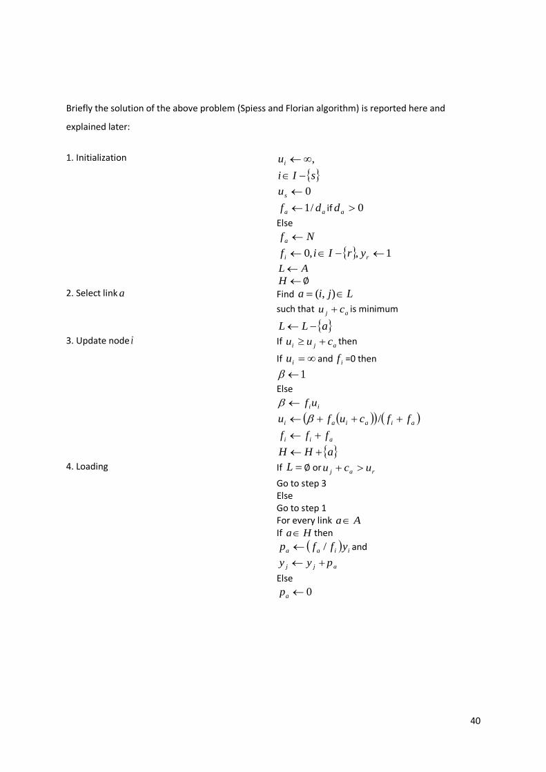
Briefly the solution of the above problem (Spiess and Florian algorithm) is reported here and
explained later:
1. Initialization ,iu
sIi
0su
aa df /1 if 0ad
Else
Nfa
1,,0 ri yrIif
AL H 2. Select link a Find Ljia ),(
such that aj cu is minimum
aLL
3. Update node i If aji cuu then
If iu and if =0 then
1
Else
iiuf
aiaiai ffcufu /
aii fff
aHH
4. Loading If L orraj ucu
Go to step 3 Else Go to step 1 For every link Aa If Ha then
iiaa yffp / and
ajj pyy
Else
0ap

41
The hyperpath between the source r and the target s can be determined as the minimization of
the following expression:
ca paaA
wiiI
This is nothing different from the expected time to conclude the calculated route. ap Is the
probability that a certain link a may be used; being a probability it is expressed as a number between
0 (impossible to happen) and (certain to happen).
pa 0 aA2
For the minimization the expression of the objective function has to follow the condition
(constraint):
pa da wi aAi i I 3
Which means that for all links a out of node i in exam (and for all nodes of the network
analysed) is guaranteed that the use of a link is inversely proportional to its maximum delay.
It is being recalled that, if a link is selected to take part in the hyperpath, then its probability
pa is over zero, otherwise, if not selected, pa is zero.
The last constraint to the objective function is the following:
paaAi
paaAi
gi i I4
2 First constraint of the objective function 3 Second constraint of the objective function

42
This relationship is equal to 1 when the node i is the source node r; results instead -1 when
i is the target node. In all other cases ig is always zero. The significant of this expression is
that the sum of the probability of the links out of a node i is equal to the probability of the
links into i and both sums have to be equal to 1.
This equation can result simpler than it seems. Assuming that an event is certain when the
probability is 1 and impossible when the probability is 0 we can make the following
thoughts: If a node is connected to the path assuming you have Ai
( i is the target node) in
the network, there is for sure the possibility you can reach the target (so you have possibility
1). So, summing all ap of links into the target node the possibility to arrive there has to be
equal to 1 since there in no point in going nowhere else once arrived to the destination. The
same thing works for all links out of a node i Ai
and thus the origin node. If a node is
connected to other links out of i , then the probability to be able to leave this node is sure so
the sum of all ap in this case is 1. We have the same probability to reach or leave a node
once we have links out of node i . This is how we can now tell that the difference ig between
the two sums (the one for all links into node i Ai
and the one for all links out of node i Ai
) is zero. We talk about sum because is performed an “OR” execution. For example if my
desire is to know the probability to arrive to a node i that has three links leading to it with pa
0.5, 0.25 e 0.25, the answer I seek to have is “Which is the probability to arrive to node j
through any of the links, link 1, link 2, link 3”. In statistics the keyword is “OR” and
mathematically becomes a sum.
4 Third constraint of the objective function

43
After that being stated, we can now see the Flow Chart of the proposed algorithm. This algorithm is
working outwards from the target so we depart from the destination s and we come back to find
the starting point r . This means that I have to pass through from s all links ( Ai
) coming to the
node in exam. The algorithm results iterative (repetitive) which means it has to execute a certain
operation more times until it satisfies certain conditions (explained next), that means that arrived in
convergence. Any iterative algorithm respects the following layout:
1. Initialization of some criteria, 2. Execution of an operation that is being repeated more times,
3. Control after every interaction of the point 2 if arrived in convergence, 4. If arrived in convergence results are being saved. If not you return to point 2
In our case we depart from the target s and the variables are being initialised in the following way:
ui, i I s , us 0
This means that we assign at all nodes of the network except from target s value iu equal to
infinity. In other words we initialize the time that remains for the arrival to the destination
from every ode i which in the beginning is a big number since we do not have an indication
about the remaining time at this point. This value ( iu ) for the source node s is zero.
Then known the delay of every link service frequency is being calculated (as explained
before):
fa1/da se da 0 o fa N se da 0

44
More specific service frequencies are assigned to the links as maximum delays: if there is no
delay (in other words the delay is zero), we have the problem that dividing to 0 we get
infinity ( 0/1 ). This is a problem because counts with infinity give infinity. In these cases
we introduce a big number (in our case N) that replaces infinity when necessary.
It is also assigned:
fi 0, i I
This frequency f is referred to the node i and not the link a . So for every node i we have a
service frequency which is going to be updated during various interactions.
It is also assigned:
yi 0, i I r , yr1
Every node i has a value of iy equal to zero apart from the source node r which will have a
value equal to 1. This value is going to be explained afterwards.
We also initialise two sets: L and H. L in the beginning maintains all links of the network (is
the same as the set A in the beginning), while H for initialization is empty.
Step 1 (initialization) is now concluded. We continue describing all operations executed in
repeated mode (step 2) until the point of convergence. This is called iteration as said before.
During iteration is selected a link ),( jia not yet examined among all these links that lead
to the node selected. That link belongs to the L set explained before. At the first interaction
is selected the shortest link that leads to the target node. This link ),( jia shall connect a
node i to the target node ( sj ).

45
The selected link is removed from the L set and added to the H set. Remaining travel time iu
is then updated from the node i to the destination j in the following way:
ui ca da ca 1/ fa
This means that the predicted to arrive at the destination node is the “ideal” time (without
delay) ca to cross the selected link plus the maximum delay that one can find on this link ad .
The algorithm continues to return to step 1 until all links have been selected and L is empty
or aj cu is larger than ru . During the first interaction it is difficult for L to be empty; as a
result it returns to interaction selecting another link connected either to the node i already
in exam or another “new” node not yet under exam. A formal and more correct expression
of how the system works is explained later.
Variables and controls that take into consideration that e certain node has been examined
are needed. In the beginning, all nodes during initialization step report a value of ju equal
and a value jf equal to zero. For the “best” link ),( jia is verified that:
ui u j ca ( iu Is from now on called acceptation standard)
If the node analysed has never been examined, ju is still equal to infinity, so the above
condition is for sure verified. In such case we also have 0jf in initialization. For ju
and 0jf we set:
1

46
In contrary, if the node has already been examined but we still have
ui u j ca we set:
ui f i
Variable is used to carry out the update of the node automatically. The acceptation
standard not only permits to verify if a certain node has already been analyzed, but also,
modify the node’s values, only if the added link permits a reduction of the forecast time to
reach the target s from the node under exam i If the acceptation standard is not satisfied,
the selected link is removed from the L set and added to the H set and the algorithm
searches for another link leading to i among the ones not yet examined (that take part of
the L set). The update now uses the following rule using value:
ui fa u j ca
f i fa
For 1 and 0if things are quite simple:
ui fa u j ca
f i fa
1
fa u j ca da u j ca
While if I have already used node i and values ju and
jf have to be updated I use the
condition jj fu (with * are indicated the updated values):
ui*
f i ui fa u j ca f i fa
f i* f i fa

47
Flow chart of the Spiess and Florian algorithm (1989)

48

49
Chapter 4
Facility location concept
Facility location, also known as location analysis, is a branch of operations research and
computational geometry concerning itself with mathematical modelling and solution of
problems concerning optimal placement of facilities in order to minimize transportation
costs, avoid placing hazardous materials near housing, outperform competitors facilities,
etc.
Location problems deals with the problem of sitting a set of supply facilities to serve a given
demand so as to optimize a certain objective function. The literature on location analysis is
very large: Already three decades ago an international bibliography mentioned more than
1,500 references (Domschke and Drexl, 1985). Therefore in the following description of
problems only seminal papers are referred to. ReVelle and Eiselt (2005) and ReVelle et al
(2008) constitute recent and insightful starting points to approach the field. Location
problems are defined either in d-dimensional real spaces and or in networks. Both classes
include continuous and discrete problems: In continuous problems there is no constraint on
the location of the facilities, in discrete ones only a limited number of potential locations are
considered.

50
Three main families of network problems can be identified according to the objective of the
optimization: minisum, minimax and coverage. The aim of minisum problems is to localize a
set of supply facilities and to assign them a set of demand points so that the total cost of
connecting demand and supply is minimized.
Different constraints give rise to different problems: In p-median problems the location of p
facilities is sought that minimize the weighted distance of the facilities from a set of n
demand points (Hakimi, 1964, 1965; ReVelle and Swain, 1970). In the simple plant location
problem (SPLP, also known as uncapacitated location problem – ULP) the objective is to
minimize the weighted distance between supply and demand but the number of supply
facilities is endogenous (Balinski, 1965).
In the capacitated plant location problem (CPLP) capacity constraints on the facilities are
considered. To the class of minimax problems belongs the p-centers problem, whose
objective is to minimize the maximum distance between the demand nodes and the supply
points to which they are allocated (Kariv and Hakimi, 1979). A third family of location
problems arises around the concept of covering: A demand point is covered by a supply
facility if their distance is smaller than a threshold value. In the location set covering
problem (LSCP) the objective is to minimize the number of facilities needed to fully cover
the demand (Toregas et al., 1971).
In maximum covering location problems (MCLP), a limit on the number of supply facilities
exists and the objective is to maximize the covered demand (Church and ReVelle, 1974). The
location of emergency services can give rise to different kinds of problems depending on the
service under planning and on the existing constraints: To mention only some of the most
recent references, minisum approaches are used when the overall or average accessibility is
crucial, e.g. in facing floods (Chang et al., 2007), in positioning emergency vehicles on urban
networks (Geroliminis et al., 2009), in locating strategic national stockpiles (Jia et al., 2007b),
in deciding on facility location and on acquisition and stocking of commodities for disaster
response (Rawls and Turnquist, 2010) . Location of sites for homeland security (Bell et al.,
2011) and facilities for general large scale emergencies (Huang et al., 2010) have been
studied through minimax location problems, which can be seen as aiming to maximize the
lowest level of service provided by the system.

51
Covering approaches are very common in emergency facilities location models: e.g. maximal
covering has been pursued in dealing with humanitarian relief chain (Balcik and Beamon,
2008) and medical supplies for large scale emergencies (Jia et al., 2007a).
A higher degree of uncertainty in demand of services and availability of resources makes
problem solving more challenging in the field of the emergency logistics than in that of the
ordinary logistics (Balcik and Beamon, 2008; Sheu, 2007). Non-deterministic location
problems have been studied both in contexts in which the probability distributions of the
quantities involved in the optimization are known (stochastic optimization problems) and in
cases in which no information on probabilities is available (robust optimization problems).
Robust optimization seems to be more suitable in dealing with natural disasters, for which
no reliable probability distribution of damages usually exists. In robust optimization the
objective is typically to minimize the cost or the regret in the worst situation, but also
different concepts of robustness have been developed. Both best-worst5 and alternative
models are presented and discussed by Snyder (2006), which remarks that the best-worst
cost approach is reasonable in facing emergencies where a high performance is required
from a system in the worst situation. Best-worst location problems are difficult to be solved,
thus exact solutions to p-median problems using this approach have been provided only for
networks with special structures or for single supply facility cases. Heuristic solutions are
available for general formulations. In most models uncertainty is related to link costs and
node weights.
The method we propose deals with the former source of uncertainty. Theoretical
contributions to best-worst p-median problems under similar assumptions have been given
by Averbakh (2003), Burkard and Dollani (2001), Chen and Lin (1998), Serra and Marianov
(1998), Vairaktarakis and Kouvelis (1999). All these studies focus on regret minimization in
1-median problems on trees. Recently Nikoofal and Sadjadi (2010) proposed a mixed integer
Robust optimization problems tackled trying to optimize the system performance in the most
adverse case are referred to as “minmax” problems by Snyder (Snyder, 2006). Here “best-worst” has
been preferred to avoid confusion with the family of problems to which the p-center problems
belong. Note that in the context of robust optimization, p-center problems can be dealt with a best-
worst approach (Averbakh and Berman, 1997; Averbakh and Berman, 2000).

52
linear formulation of robust p-median problems which allows for different levels of the
conservatism regarding the link lengths, whose intervals of values are assumed known.
Most location problems on general networks are NP-hard and many research efforts have
been put in place to develop tractable and reasonably approximate solution methods
(ReVelle et al., 2008). It has been shown that p-median problems can be solved in
polynomial time if p is fixed or the graph is a tree (Garey and Johnson, 1979). Several
approaches have been brought forward to solve p-median problems: enumeration and
heuristics, linear programming relaxations, meta-heuristics and approximation algorithms
(Reese, 2006). Greedy (Kuehn and Hamburger, 1963), Alternate (Maranzana, 1964) and in
particular Vertex Substitution (Teitz and Bart, 1968) heuristics have proven to be very
popular and numerous improvements and hybrid formulations have been brought forward.
In the Greedy heuristic a solution is searched by iteratively modifying the set of candidate
facility locations so that the change in the goal function is optimized. This can be done
following an Add or a Drop procedure (Sridharan, 1995). In the latter case the search starts
locating a facility at each potential site and progressively removes facilities (until the
solution set contains p nodes) so as to minimize the increase of the objective function
(Feldman et al., 1966). Improvements to the Drop procedure for non-capacitated problems
have been proposed by Whitaker (1981) in which at each iteration k facilities are eliminated
and k-1 reintroduced.
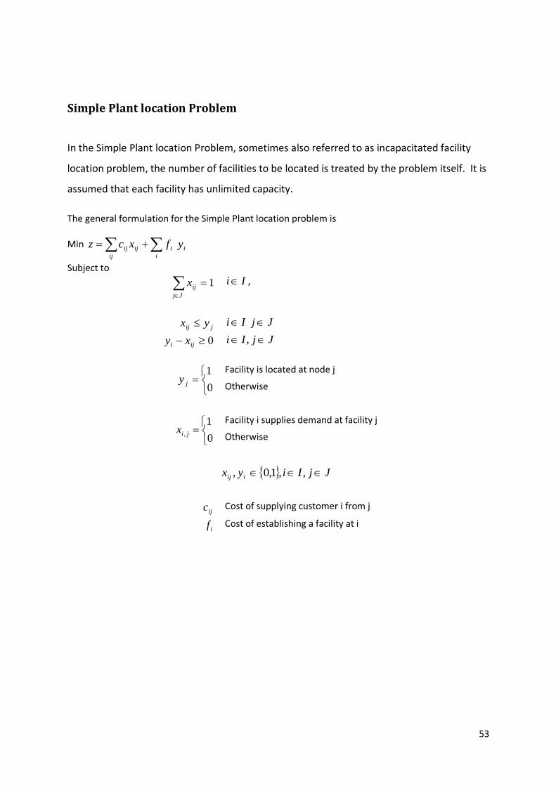
53
Simple Plant location Problem
In the Simple Plant location Problem, sometimes also referred to as incapacitated facility
location problem, the number of facilities to be located is treated by the problem itself. It is
assumed that each facility has unlimited capacity.
The general formulation for the Simple Plant location problem is
Min i
ij i
iijij yfxcz
Subject to
Jj
ijx 1 Ii ,
jij yx Ii Jj
0 iji xy JjIi ,
0
1jy
Facility is located at node j
Otherwise
0
1, jix
Facility i supplies demand at facility j
Otherwise
JjIiyx iij ,,1,0,
ijc
Cost of supplying customer i from j
if Cost of establishing a facility at i

54
Capacitated plant location problem
In the Capacitated plant location problem it is assumed that each facility has limited
capacity. These problems are mostly solved by Lagrangian relaxation methods or the matrix
column generation method.
Let iI ,...1 give potential facility locations providing a service of a certain value or
producing a product of a certain value. Let 0ic be the establishing cost of the location
among the Ii potential facility locations provided and 0iV V the value of the produced
service or product.
Let jJ ,...,1 assign users that require service. For each pair i, j let 0, jig be the
production and transportation cost and 0, jig the value of service (or product) created in
facility i directed to the user j .
Then we have
0
1jy
Facility is located at node j
Otherwise
and
0
1, jix
Facility i supplies demand at facility j
Otherwise
Then the Capacitated Facility Location Problem may be written
iiij
Jj
ij yVxp
Ii
Ii Ii Jj
ijijii xgycmin
Ii
ijx 1 Jj
JjIiyx iij ,,1,0,

55
Location set covering problem
The location set covering problem treats the location of minimum possible facilities. This
should ensure that demand points do not exist outside the maximum distance that a facility
serves. When solving the set covering problem over a range of values it is possible to
produce a cost effectiveness curve between the maximum service distance and the distance
from a facility.
The only decision process used in the location covering problem is the number of facilities in
terms of a cost factor. In this way (isolating a discrete number of facilities) it is possible to
give the solution for many real world formulations.
The examination of the cost effectiveness curve shows that for a certain number of facilities
there may be more than one solutions that fulfill coverage requirements. When there are
specific numbers of facilities, it is possible to take the solution that uses the maximum
service distance.
Maximum covering location problems
The maximum covering location problem is stated as the "Maximize coverage (population
covered) within a desired service distance S by locating a fixed Number of facilities" (Richard
Church, Charles ReVelle, 1971). In the same paper the problem is designed as the "Maximal
covering location problem with mandatory constraints" stated as locating a fixed number of
facilities in order to maximize the population covered within a certain service distance S,
while maintaining mandatory coverage within a distance T (T>S).
The solution techniques to solve such Maximum covering location problems consist of
Heuristic approaches or linear programming. We only name two heuristic approaches to
solve such problems. These are the Greedy Adding Algorithm (GA Algorithm) and the
Greedy Adding with Substitution Algorithm (GAS Algorithm). These two methods cannot
however guarantee a global optimality solution.

56
If we consider a network of nodes and arcs the mathematical formulation of the maximum
covering problem is:
Maximize
Ii
ii yaz
i
Nj
i yxi
For all Ii
Px
Ji
i
1
0jx
Service located at node i For all Jj
otherwise
1
0iy
Population served at node j For all Ii
otherwise
I : Set of demand nodes
J : Set of facility sites
S : Distance beyond which a demand point is considered uncovered (S value can be chosen differently for each demand point)
ijd : Shortest distance from node i to node j
iN : SdJj ij
ia : Population to be served at demand node i
p : Number of potential facilities to be located

57
Chapter 5
The mixed strategy
Both hyperpath and facility location concept are involved so as to provide a mixed strategy.
The problem is solved in two steps. First we use all possible routes to calculate minimum
paths. Then, according to the rescue centres or terminal points we wish to use (exact
number of rescue centres or terminal points), we locate them along the road network in
basis of the risks the driver may find ehen he seaks to reach his final destination.
Description
The algorithm was initially developed to optimize a rescue plan towards populations hit by a
natural disaster such as an earthquake. However it seems that it applies more to the flood
problem following reasonable implementation steps showed later. The principal target is to
individuate along the road network optimum, valid places in which to locate centres of
human relief against a natural disaster. In such centres, there have to be enough necessary
supplies in order to support the total number hit by an earthquake.
More specific along the road network, close to the areas hit by the natural event, there are
individuated specific nodes where population is supposed to be located. Those nodes (or
points) are referred to as population centres and with each one of them, there are

58
associated attributes, such as the number of inhabitants each population centre has,
specifically called his. Those represent exactly the set of nodes from which we will select our
potential rescue centres. At the end of the execution of the algorithm, some population
centres become rescue centres, which means that corresponding to these points there are
resources predisposed to rescue all populations hit by the natural disaster.
The optimization of the rescue plan, apart from the indication of rescue centre locations,
also calculates which population is assigned to each rescue centre as well as a list of possible
paths which vehicles can use in order to connect rescue centres to population centres.
We note that we individuate a list of paths or routes because we calculate all possible paths
from a rescue centre to a population centre. Very often it is proposed that only one route
be calculated, the shortest one, independent of the risks a driver may find along his trip.
This list of paths, namely haperpath, which emanates from the field of transit assignment of
transport engineering, is a set of routes any of which may be optimal. Using the haperpath
as the approach to the solution, for the treated problem we offer valid alternatives in case
part of the road network may become unusable. The selection of these paths is calculated
on a probabilistic basis seeking in each case to select the next link by minimizing the risk the
driver might be exposed to.
In order to correctly execute the algorithm there are some constraints which need to be
respected. First and foremost, the number of potential rescue centre locations need to be
determined beforehand. Secondly, each rescue centre needs to have limited capacity,
which is specifically stated. This means that we have determined the maximum number of
people that each rescue centre can support (zr value), at initialization. Last but not least,
each population centre has to be assigned to one and only one rescue centre while one
rescue centre can serve more than one population centre.
Implementation steps
In order to efficiently apply the proposed procedure in the case of flood it was necessary to
proceed with some modifications and see the problem from a different point of view as well
as involve a different phase of emergency management. In the case of flood, in fact, we

59
consider an evacuation plan, initially before the arrival of the flood wave, rather than a
rescue plan. We could also consider both an evacuation plan (for the mitigation and
preparedness phase of emergency management) and a rescue centre location plan so as to
reach populations hit by the flood after the flood wave has passed (relief phase of the
emergency management).
In order to correctly state an evacuation plan, starting from the problem already described,
we need to replace rescue centres with terminal points and optimize the flow from
population centres to the related terminal points. In these potential terminal point
locations, all responsible citizens who decide to follow the instructions provided by the local
civil protection may have to spend a long period of time away from the disaster zone. These
potential terminal point locations have to be already stated beforehand, by the local civil
protection department, responsible for the area referred to.
We still have to individuate specific points (nodes) where population is concentrated. These
nodes are referred to as population centres. Furthermore, we add a set of nodes which are
candidate locations to become terminal points. In contrast to what we propose for the
earthquake problem, only some of these later nodes described, can be selected as potential
terminal point locations. Naturally, it is impossible to locate terminal points, where
population centres are located for flood responses. This is what we propose for the
earthquake rescue centre location problem: rescue centres, which have the role of terminal
points in cases where we need to evacuate before a flood emergency, cannot be in the area
where flood waters may appear. They have to be away from the crisis area, at a 'dry' secure
place.
For an emergency evacuation plan before a flood, terminal-rescue locations are particular
population centres that have no permanent inhabitants in the sense that no population
intends (or needs) to leave that place during flood evacuation. This means that we set value
hs equal to zero. Population centres are treated in a particular way as well; they do not have
rescue capacity, which means that we assign a null value to zr attribute. This value indicates
the number of people each rescue centre can support. In this way we can apply the same
macro-methodology to treat both floods and earthquakes during different phases of
emergency management.

60
In conclusion, within this work, we propose an evacuation plan during the preparedness or
mitigation phase of emergency management. Experimentally, we suggest a rescue plan,
after an earthquake which applies to relief phase of emergency management.
Results however are completely different when we treat a flood emergency compared to a
post earthquake emergency. In the first case, we refer to citizens who seek to leave
population centres in order to reach terminal points. In the second case, rescue vehicles
take advantage of the haperpath concept in order to use all possible paths to reach
populations affected by the consequences of a vulnerable earthquake zone.

61
Chapter 6
Flood responses
We propose here a method for the positioning of terminal points organized to gather
people after emergencies generated by floods. The demand points are referred to as
“population centers”. The candidate locations for terminal points coincide with the nodes of
a transport network which can be blocked homogenously by the disaster. A flood model
(like the one generated by Francesco Dottori called CA model) can make possible the
estimation of the maximum additional cost (or delay) for each link caused by the disaster.
The problem is formulated as a two stage optimization problem: The primary problem is a
capacitated p-median problem in which the location of p rescue centers is sought which
minimizes the overall weighted best-worst cost between population centers and terminal
points. In the secondary problem the best-worst cost between each pair of terminal points
and population centres is worked out as the payoff of the mixed strategy Nash equilibrium
for a non-cooperative zero sum game between citizens seeking to reach terminal points and
node-specific evil entities able to spoil a single link at each node.

62
General Description
We consider a road network composed of a set of links Aa that represent the streets and
a set of nodes Ii that represent the junctions of the network (Figure 6-1). Among these
nodes i we identify a subset IR of nodes where we consider the location of points
referred to as terminal points of the network and a subset IS of nodes where we
consider the location of points referred to as population centers.
Figure 6-1 TeleAtlasTM sample map - representation of a road network. The nodes are the junctions and the links are the streets of the transport network
In the proposed system, we assume that the population exposed to the catastrophe is
located at a subset of nodes S, referred to as population centres. We also assume that local
civil protection has proposed possible locations referred to as terminal points. We wish to
reach these nodes from rescue centres. This study examines the case where rescue centres
have an upper limit on the population each can cover and resources are sufficient for only m
rescue centres, where m is sufficiently large to cover the entire exposed population. The

63
problem is to find the best subset of nodes R S at which to locate the m rescue centres.
We then describe below three possible ways to solve this problem according to the time
local civil protection has decided to communicate the state of emergency; a lot of time
before the mass of water is about to arrive, during the emergency state or after the
catastrophe, considering that both rescue vehicles have to circulate and, when possible,
stranded civilians need to find another place to stay until the complete recovery of the
district.
We assume that every link has a cost of use ca before the catastrophe. Before, during or
after the catastrophe, there is an additional cost of da calculated differently depending on
the time local civil protection decides to announce the state of emergency. Yet, we are
almost certain as to which links are degraded. We estimate the process of the links
degradation using a flood inundation we describe later. Suppose we are seeking to access
rescue centre r from node s. We assume that upon exiting any node i en route to r one link
is degraded. Given the additional costs for these links when degraded, we seek the set of
potentially optimal paths from node i to destination s for the worst case set of link failure
probabilities. The set of potentially optimal paths between rescue centre r and destination s
is referred to as a hyperpath. Given the worst case link failure probabilities, we calculate link
usage probabilities, which minimise the expected hyperpath cost, urs, and then use the
expected hyperpath cost for determining the optimal deployment of rescue centres.
More specific, Figure 6-5 describes the input data the proposed system needs. A street map
where the streets are represented as links and the junctions as nodes Figure 6-5 (a) , a
subset of nodes where population is located Figure 6-5 (b) and a subset of nodes where
terminal points are located Figure 6-5 (c). The system, first calculates all possible paths the
civilians can use during the evacuation plan we propose. It then identifies the optimum
terminal points, among the ones the local civil protection district has proposed, they can use
according to the actual state of the flood status. We distinguish three different possibilities
of flood emergency according to the time the alarm may be communicated to civilians.
The terminal point location problem is divided into two problems which may be solved
separately. First, the minimum hyperpath costs are found from each population centre to all
terminal points. We create a matrix in which are captured the hyperpath costs in travel time

64
units from each population centre to all terminal points. Then this matrix is used to solve
the rescue centre location problem which has two sets of decision variables, namely x,
which represents the decision to supply a given population centre from a given rescue
centre, and y, which represents the decision to locate rescue centres at given nodes. The
constraints ensure that each population centre is covered by one and only one rescue
centre and that the maximum population that a rescue centre can cover is not exceeded.
The degradability of the network means that travel costs are not known with certainty but
estimated with several methods we describe later. We assume that upon arrival at every
node en route to a destination the preferred exit link from that node may be degraded or
indeed blocked. For link a, da measures the degradability of the link which is stated as high
(almost infinity) when the link is partly or completely blocked or has various values
according to the actual state of the flood and the time it is estimated to arrive. Where this is
low, the incentive for finding an alternative route is correspondingly low. A very large value
for da would correspond to the case where link a is very likely to block soon (e.g. in less than
five hours time) therefore the driver is exposed to high risk and an alternative must be used.
Using various techniques to decide if a link may be open or closed at a certain time, we can
be almost certain of the level of degradation of the link. This delivers the set of paths from
each origin to each destination that may be optimal if one and only one link exiting each
node is degraded as well as the expected travel time corresponding to pessimistically
estimated link failure probabilities.
So far, we have described some main input values we use to calculate the emergency paths:
ca which captures travel time of link a in travel time units and da calculated in the same
travel time units, which captures the additional delay on a certain link ɑ caused by several
reasons. This can be generated as the evacuation time estimate which is the time required
to move the population at-risk out of the evacuation area. This has to take into
consideration also human factors such as mobilization time and evacuation response as well
as human psychological states during an emergency. In this study, we calculate delay travel
time
The method used to calculate a vulnerability index for each link was based on developing
indicators for the blocked passage due to the time the water is expected to arrive at a

65
certain link. Furthermore, the capacity of the road network is also considered by following
the multinet TeleAtlasTM street classification and the speed limit of each link.
There are also other important attributes that we take into consideration. Firstly, the
maximum capacity each terminal point can support (zr) since in maximum covering location
problems (MCLP), a limit on the number of supply facilities exists and the objective is to
maximize the covered demand (Church and ReVelle, 1974). Secondly, we set the number of
people each population centre has. This is all public information provided by local
government offices.

66
Figure 6-2 (a) Sample of a street map (TeleAtlas streetmap), a representation of a road network
Figure 6-3 (b) ) Terminal points: purple points represent terminal point locations

67
Figure 6-4 (c) Population centers: green points represent population centre locations
Figure 6-5 Input data for the proposed system, (a) Sample of a street map (TeleAtlas streetmap), a representation of a road network, (b) Terminal points: purple points represent terminal point locations, (c) Population centers: green points represent population centre locations
Cellular automata Flood Propagation Model
The inundation model we use to identify beforehand the roads that may be closed in the
course of flood waves is the Cellular Automata 2D Model produced by F. Dottori, E. Todini.,
2011. This is a model based on the cellular automata approach and improved through the
implementation of two techniques; an inertial formulation for the computation of
discharges, originally developed for the LISFLOOD-FP model by Bates et al. (2010); and the
incorporation of a local adaptive time step algorithm, based on a technique originally
presented by Zhang et al. (1994).
A cellular automata is a discrete choice model (i.e. when individuals have to select an option
from a finite set of alternatives). This great chapter of methodologies apply to a lot of
disciplines such as mathematics, physics, complexity science, theoretical biology,
computability theory, microstructure modeling as well as fluid dynamics phenomena such as
debris flows (D'ambrosio et al., 2003)

68
More specifically, this model describes the physical dynamic systems in a discrete way
regulated only by local laws. Generally, it is made of a regular grid and can be in any finite
number of dimensions. Every cell is in the state "on" or "off" in respect to its
properties."Neighborhood" is defined as the neighbour cells which are usually the cells that
include a certain cell. Initially it is assigned a condition for every cell after selecting the initial
state and then, following a fixed rule, generated mainly by a mathematical function, the
new state of each cell is produced depending on the actual condition both of itself and the
"neighborhood" - the neighbour cells. The updating rule of every cell does not change over
time.
This model uses the macroscopic cellular automata approach to represent flood plain
inundation events where diffusion phenomena are dominant. The macroscopic CA approach
partly differs from the classical CA approach structure described so far. Every single cell
represents a volume of fluid to which the momentum and continuity equations may be
applied. The cell lattice forms a grid of polygonal elements of either regular or variable
shape and dimension, which represents the topography of the study area.
The adopted computational scheme can be described through the finite volume
schematization. According to Garcia-Navarro and Murillo (2010), considering a single finite
volume we can consider the following equation
SFt
W
Equation 1
Notation W : conservative variables t : time F : flux function S : source term

69
Following a two dimensional cell-centered finite volume scheme, Equation 1 is integrated in a
volume or grid cell Ω:
SdFdWd
t
Equation 2
In the CA model scheme originally proposed by Dottori and Todini(2010) W : the volume of water, V, stored in a cell F : total discharge Q between cell i and the adjacent cells m, per unit width
Taking into consideration this notation Equation 2 gives the solution at cell i at time level t+Δt.:
tm
j
t
ji
t
i
tt
i qQtVV
1
,
Equation 3
Δt : time step in use q : total discharge entering or leaving the domain through the cell i
The integration in time is obtained with the Euler explicit scheme, following the CA rule that the
overall system state depends only on the previous time step.
If we consider two adjacent cells i and j, discharge Q is calculated using the momentum equation
leaving, in time and space, the variation of velocity along the relevant direction:
2135
,
x
HH
n
bhQ
jim
ji
Equation 4
Hi : water stage in level i Hj : water stage in level j Δx : distance between centroids of the two cells B : width of the contact face N : Manning roughness coefficient hm : arithmetic mean between water depths in the two cells

70
We note that the proposed computational scheme is equivalent to a pipe network, where
nodes represent the cells and the links represent contact faces. In this way, any generic 2D
flow breaks up into 1D flow components through the links. The momentum equation is
integrated along the link direction Δx being a vector with x and y components. Every flux
component is then decoupled from the others , in a way that Equation 4 can be solved
separately for every link.
The final CA model we used, inspired by cellular automata approaches, resembles various
modelling techniques especially the part of the storage cell approach. The most
commercially popular models based on this technique are LISFLOOD-FP (Hunter et al., 2005)
and FLO2D (FLO-2D Software Inc., 2007). They both perform flux computation through the
decoupling of x and y flow components. LISFLOOD-FP uses Equation 4 for discharge
computation while FLO2D uses the full dynamic momentum equation.
However, we suggest the use of this flood model for a number of reasons. Firstly, the
introduction of a tool, namely "pre-processor" that allows the use of regular grids derived
from digital elevation models (DEM), as well as polygonal grids from TIN files. The code
structure (that requires this special tool mentioned above) allows within the same model
the use of both regular and irregular mashes. From the users point of view and for the
needs of this study, this method is very efficient. Secondly, the similarity of the
computational scheme to a pipe network gives an advantage to the computational scheme
of the structure of the code; node and link elements all share computational information.
This leads to major code efficiency. Last but not least, focusing on the flux computation
between cells, different formulations for computing the friction slope along the links were
considered and tested for use in the CA model.

71
Evacuation plans
Emergency evacuation is the immediate and rapid movement of people away from the
threat or actual occurrence of a hazard. Examples range from the small scale evacuation of a
building due to a bomb threat or fire to the large scale evacuation of a district because of a
flood, bombardment or approaching weather system. In situations involving hazardous
materials or possible contamination, evacuees may be decontaminated prior to being
transported out of the contaminated area.
Static pre-flood evacuation
In this paragraph is described an emergency evacuation plan is described in which it is
assumed that the state of emergency has been announced in time and thus citizens have all
available time to evacuate the city. At this particular stage all streets are open and there are
no streets closed because of the flood.
We first solve the secondary minimisation problem which finds the hyperpath costs from all
origins referred to as "population centres" to each destination referred to as "terminal
points" for the network under the state of emergency. In Figure 6-12 we present a detailed
representation of all optimal paths from all six population centres to one terminal point
respectively.

72
Figure 6-6 (a)Demonstration of all available paths from each population centre to terminal point No "1"
Figure 6-7 (b) Demonstration of all available paths from each population centre to terminal point No "2"

73
Figure 6-8 (c) Demonstration of all available paths from each population centre to terminal point No "3"
Figure 6-9 (d) Demonstration of all available paths from each population centre to terminal point No "4",

74
Figure 6-10 (e) Demonstration of all available paths from each population centre to terminal point No "5"
Figure 6-11 (f) ) Demonstration of all available paths from each population centre to terminal point No "6". Figure 6-12 Static pre flood evacuation emergency plan . There are not blocked streets due to the emergency because the alarm was announced on time before the evacuation (time local civil protection decides). (a) Demonstration of all available paths from each population centre to terminal point No "1", (b) Demonstration of all available paths from each population centre to terminal point No "2", (c) Demonstration of all available paths from each population centre to terminal point No "3", (d) Demonstration of all available paths from each population centre to terminal point No "4", (e) Demonstration of all available paths from each population centre to terminal point No "5", (f

75
We then calculate the hyperpath travel cost matrix from each population centre to one
terminal point every time. Figure 6-13 shows such a result for the pre flood condition. We
can understand that travel costs are more sustainable when vehicles can circulate through
the network when all streets are available.
To avoid traffic congestion during the evacuation we assume that pedestrians are served by
public transport (e.s. public buses) and the rest of the vehicles use all available paths already
calculated. The evacuation travel time depends primarily on the relationship between traffic
demand and road capacity (supply). When transport demand exceeds transport capacity
over a particular time period, travel speed declines and traffic environment exhibits
queuing. This is characteristic of congested conditions where the result is that traffic moves
very slowly. These relationships (supply and demand) exceed the needs of this research. We
assume that supply and demand are constant considering that people would use public
transport to evacuate rather than personal vehicles. It is also assumed that public transport
is well organized and follows the instructions of the local civil protection.
Figure 6-13 Hyperpath costs, evacuation before the “flood wave" - Static Version -Time in seconds

76
Having found the minimum hyperpath costs, we can now solve the rescue centre location
problem. This is a form of the Set Covering Problem (SCP), since each terminal point covers a
set of population centres and we are looking for the assignment of terminal points to
minimise expected travel costs. This is a complex problem as the number of ways that m
locations can be selected from n sites is ! !( )!m n n m , although the maximum population
coverage constraint imposed on each terminal point will reduce this number.
For the solution of the terminal point location problem we propose a greedy heuristic.
Initially, both population and terminal points are considered terminal points. Every point is
assigned to itself. There are as many terminal points as there are population centres plus
terminal points and the expected travel cost F is zero. The algorithm repeatedly removes
one terminal point. When a terminal point is removed, each population centre assigned to it
is reassigned to the nearest remaining terminal point that has sufficient capacity. The extra
expected travel time resulting from the reassignment of destinations is calculated and the
terminal point that causes the least extra travel time is removed. F is then increased by the
amount of extra travel time. Terminal points continue to be removed until all population
centres are assigned to terminal points.
Figure 6-14 represents the result of the solution of the primary location problem where population
centres are assigned to their related terminal points.
Figure 6-14 Assignment of population centres to their related terminal points.

77
Static post-flood evacuation
In this paragraph is described an emergency evacuation plan is described in which it is
assumed that the state of emergency has been announced late and thus citizens have very
few time to evacuate the city. At this particular stage there are a lot of closed streets and
people have very few available possibilities to evacuate if not completely blocked by the
flood.
As for the static pre-flood solution of the problem we calculate the hyperpath travel cost
matrix from each population centre to one terminal point every time. In Figure 6-21 we
illustrate the paths from all population centres to one terminal point respectively. Travel
costs in this condition are not sustainable since vehicles have to avoid blocked links and
reach their destinations after long journeys.
We set ca value as the travel time of link a. We also set da value equal to infinity since we
assume all links the flood wave reached are blocked.
Figure 6-15 (a) Demonstration of all available paths from each population centre to terminal point No "1"

78
Figure 6-16 (b) Demonstration of all available paths from each population centre to terminal point
No "2"
Figure 6-17 (c) Demonstration of all available paths from each population centre to terminal point
No "3"

79
Figure 6-18 (d) Demonstration of all available paths from each population centre to terminal point
No "4"
Figure 6-19 (e) Demonstration of all available paths from each population centre to terminal point
No "5"

80
Figure 6-20 (f) Demonstration of all available paths from each population centre to terminal point
No "6" Figure 6-21 Static post flood emergency evacuation plan(a) Demonstration of all available paths from each population centre to terminal point No "1", (b) Demonstration of all available paths from each population centre to terminal point No "2", (c) Demonstration of all available paths from each population centre to terminal point No "3", (d) Demonstration of all available paths from each population centre to terminal point No "4", (e) Demonstration of all available paths from each population centre to terminal point No "5", (f)Demonstration of all available paths from each population centre to terminal point No "6".
Figure 6-22 illustrates the hyperpath matrix. This illustrates travel times calculated respectively from
all population centers to each terminal point.

81
Figure 6-22 Evacuation after the "flood alarm"-Static Version -Time in seconds
Having found the minimum hyperpath costs, we can now solve the rescue centre location
problem. Figure 6-23 illustrates the assignment of population centers to their terminal points.
Figure 6-23 Assignment of population centres to the optimum terminal points after the "flood wave"-Static Version

82
Dynamic, In motion evacuation
For the dynamic solution of the problem we propose two methods that both depend on the decision
of da value described previously. The areas that are more likely to manifest delays have a higher
delay and alternative paths have to be found in order to avoid them. We have calculated these areas
with the cellular automata CA2D flood model described before capturing the flood extension every
five hours. Figure 6-28 illustrates the calculation in four consecutive stages for the catastrophic flood
that took place in Alessandria, Piedmont Region in Italy, 2 - 6November 1994.
Figure 6-24 (a) two hours after the beginning of the flood

83
Figure 6-25 (b) four hours after the beginning of the flood
Figure 6-26 (c) six hours after the beginning of the flood

84
Figure 6-27 (d)eight hours after the begining of the flood Figure 6-28 CA2D flood plain model: CA2D model interpretation two hours after the beginning of the flood (a), CA2D model interpretation four hours after the beginning of the flood (b), CA2D model interpretation six hours after the beginning of the flood (c), CA2D model interpretation eight hours after the beginning of the flood (d)
As mentioned before, we consider two different ways to calculate both the set of optimum paths
from the population centers to the related terminal points and incidentally the assignment of the
population centers in a second step.
The first solution we propose resembles the static version since we give fixed da values to four
different areas as calculated by the cellular automata (CA2D model). At the moment da values are
calculated in terms of the speed limit of a certain link a da =ca/speed limit of link a. We add to the
previous calculated da value a constant number that would increase da value 30 times in the area
which is about to be affected by the flood wave after 5 hours. We make the same consideration for
the areas that will be affected after 10, 15 and 20 hours , increasing 5, 3 and 1 times respectively to
the zones already calculated by the catastrophic event Figure 6-29
We then calculate travel times (travel time matrix or hyperpath costs table) which we use to solve
the terminal point location problem and assign the population centers to the best terminal point in
terms of ease of reach. Hyperpath costs matrix for this solution is reported in Figure 6-30. The
assignment of the population centers to the related terminal points is illustrated in Figure 6-31

85
Figure 6-29 Flood evolution of the "Alessandria 1994" event according to CA2D flood propagation model
Figure 6-30 Travel times calculated from each population centre to each terminal point respectively.

86
Figure 6-31 Assignment of population centres to the optimum terminal points according to the dynamic solution with fixed da values

87
For the second dynamic solution we propose, the assignment of population centers to their
related terminal points changes according to the actual situation of the flood. To solve this
formulation, we add to the previous calculated da value a constant number that would
increase da value 100000 times. As a result, these links receive a very low probability to be
selected. At the moment da values are calculated in terms of the speed limit of a certain link
a da =ca/speed limit of link a.
When the flood wave arrives, we consider a very high number of da values for each link that
is within the flooded area calculated from the flood model the first five hours (we increase
100000 times the actual value of da). In termination of these five hours, we update the da
costs with the same value with respect to the expanded flood after 10, 15 and 20 hours
respectively as shown in Figure 6-29.
We calculate the different travel time matrixes for all four different solutions, every five,
ten, fifteen and twenty hours from the arrival of the flood wave. Having found the minimum
paths and their related travel times, we then use heuristics to find the optimum solution for
the assignment of each population centre to the closest and less risky - in terms of
alternative route finding - terminal point. These four different solutions are reported in
Figure 6-36.

88
Figure 6-32 (a) , after four hours from the arrival of the flood wave
Figure 6-33 (b) , after four hours from the arrival of the flood wave

89
Figure 6-34 (c) , after four hours from the arrival of the flood wave
Figure 6-35 (d) , after four hours from the arrival of the flood wave Figure 6-36 Assignment of terminal points to their related population centres the first two hours from the arrival of the flood wave (a), after four hours from the arrival of the flood wave (b), after six hours from the arrival of the flood wave, (c) after eight hours from the arrival of the flood wave
Case study Alessandria 2-6 November 1994
The Tanaro River entered a phase of extraordinary flooding from 4 to 7 of November 1994
with catastrophic consequences for the entire basin. As already stated, severe actual hydro

90
geological conditions, together with exceptional rains enlarged the phenomenon. During the
morning of the 6th November being aware of several flooded cities along Tanaro River(such
as the city of Asti) the flood wave arrived in Alessandria; within a few minutes streets turned
into torrents with drifting cars. By the end of the catastrophe there were also 14 victims.
Position and hydrologic conditions
The Tanaro (Tanaro drainage basin) is a 276 km long River, rising in the Ligurian Alps, adjacent to the
French border. The Tanaro River is the most important right side tributary to the Po River in terms of
drainage basin size 8293 km2, discharge and length. Figure 6-37 and Figure 6-38 illustrate the
position of the river and the extension of its drainage basin.
During the second half of October '94 the Tanaro basin was characterized by consecutive intensive
episodes of rain precipitation. This caused a high degree of saturation in the Piedmont basin the
first days of November , allowing low precipitations of rainfall to generate superficial flow capable
of seriously restricting the entire hydrologic network. Figure 6-39 illustrates the hydrologic network
and the stations of rain precipitation while Figure 6-40 reports the extreme precipitations captured
by the existing network in November '94. In Error! Reference source not found. are reported flow
alues of the day before the catastrophic day of the 4th of November 1994. It is observed that
immediately before the event the hydrographic network, with a high degree of saturation, disposed
flows of medium annual flows.
Table 6-1 Hydrological characteristics of some significant stations. Source EVENTI ALLUVIONALI IN PIEMONTE (Torino 1998)
Station Basin surface (km2) Flow 3/11/94 (m2/s)
Medium annual flow (m2/s)
Carde 510 10 11
Carignano 3804 85 71
Torino 5210 90 95
S. Martino 581 9 15
Susa 628 19 11
Lanzo 582 30 20
Mazze 3837 58 96
Borgosesia 695 80 33
Gaiola 562 20 18
Alba 3415 80 71

Figure 6-37 Position of Tanaro River basin

Figure 6-38 Position of case study
Figure 6-39 Position of hydrometric stations in 1994. Source EVENTI ALLUVIONALI IN PIEMONTE (Torino 1998)

93
(a) Cuneo (b) Alba
(c) Cardè (d) Luserna S. Giovani
(e) Lanzo (f) Susa
(g) Mazzè (h) Borgosesia
(i) Torino (g) S. Martino Figure 6-40 Perceptions of hydrometric stations of Tanaro basin during 2-6 of November 1994. Source EVENTI ALLUVIONALI IN PIEMONTE (Torino 1998)

94
Flood dynamic
The city of Alessandria was hit by the flood wave on the 6th of November after three days of
continuous rain. We can distinguish three different phases of the event: the first phase 8:30-
10:30 GTM + 1 time zone – preparedness phase, the second phase 10:30-13:0 GTM + 1 time
zone - paroxysmal phase and the third phase 13:00-14:30 GTM + 1 time zone- catastrophic
phase (source EVENTI ALLUVIONALI IN PIEMONTE 2 - 6 Novembre 1994, 8 Luglio 1996, 7 -
10 Ottobre 1996, REGIONE PIEMONTE ).
The area affected by the flood event during the first phase of the flood (8:30-10:30 GTM + 1
time zone) is demonstrated in Figure 6-28 (a). Until the first hours of the morning of the 6th
of November there were destroyed a couple of farms and cultivation areas were destroyed.
A couple of minor infrastructure failures were captured.
During the second phase of the flood (10:30-13:0 GTM + 1 time zone - paroxysmal phase)
"Orti" area plain (Figure 6-42 (d)) is gradually flooding in southwest direction. At this moment
the entire cultivation are of "Orti" was hit by the event. Furthermore there have been
captured several infrastructure failures along the river side, while water level at this stage is
4.0-5.0 meters higher than normality. "Cittdella" bridge, the older bridge of the city of
Alessandria has been already subject to various damage. However, it didn't fail.
The third and most catastrophic phase of the event was yet to come. At 13:00 GTM + 1 time
zone the junction between the railway and the highway failed and consequently caused
almost three km of damage along the railway. Figure 6-41 illustrates the failure along the
railway. During the first two phases of the event (8:30-13:00 GMT+1 time zone) the junction
between the rail way and the highway A26 (Figure 6-41) maintained the character of
"embankment" accumulating a great amount of water. Needless to say that after the failure
of the railway junction the flood wave which occurred was devastating and destroyed
almost everything along its passage.

95
Figure 6-41 Infrastructure failure during the catastrophic phase of the flood (third phase 6th of November 1994 13:00-14:30 GMT+1 )
Built-up area vulnerability
Urbanization is a long-term process of transformation from traditional to industrial
economies over time. The process of urbanization in the city of Alessandria begins at the
end of the 12th century with continuous growth until today. The city of Alessandria, situated
at a strategic position at the confluence of Bormida and Tanaro Rivers Figure 6-38 has has
grown over 12 km2 during the last two centuries. Luino F., Arattano M. and Brunamonte F.
(1994) explain the vulnerability of the city to flooding and in Figure 6-42 we report the
expansion of the city from 1851 until 1991 (Luino et al., 1994). We also report from the
same study, the urban development of the city of Alessandria over the last two centuries in
Error! Reference source not found..
The November 1994 event involving the Tanaro River was not the first catastrophic flood
ever; there have been captured a long series of flood events on the Bormida and Tanaro
Rivers. The most important goes back to 1879, when the entire plain from Asti to

96
Alessandria was flooded. However, damage was limited. In November 1994, the evident
urbanization over the recent years (occupation of the entire river–side, floodplains and
some parts of the river-bed itself, insufficient size of bridge arches, negative interference of
road and railway embankments and lack of adequate maintenance and cleaning of the
natural drainage network) led to devastating consequences.
(a) (b)
(c) (d)
Figure 6-42 Urbanization of the city of Alessandria (a) 1851, (b) 1875, (c) 1933, (d) 1991, Luino. F. et al (1994)
Table 6-2 Development of the city of Alessandria over the last two centuries, Luino. F. et al (1994)
Year Built up area in km2 Inhabitants Area (m2)/inhabitants
1828 1.00 17,225 58.1
1851 1.20 27,057 44.4
1875 1.52 30,358 50.1
1933 2.73 53,619 50.9
1991 9.47 100,523 94.2

97
Simulation of the 2nd-6th November 1994 event into CA2D model
As described in the Cellular automata Flood Propagation Model paragraph the input data
needed for the floodplain inundation model consist of an accurate Digital Elevation model
(DEM) of the area of interest and hydrometric precipitation during the event.
We collected a 90x90 meter resolution digital elevation model from the SRTM (Shuttle
Radar Topography Missions) mission. In the case of research, SRTM data is available for free.
This international project was spearheaded by the National Geospatial-Intelligence Agency
(NGA) and the National Aeronautics and Space Administration (NASA). During an eleven day
mission in February 2000 the shuttle, consisted of a specially modified radar system ,
generated on a near-global scale the most complete high-resolution digital topographic
database of Earth.
For research purposes there is also available another digital elevation model product with
30x30 meter resolution. This mission called Advanced Spaceborne Thermal Emission and
Reflection Radiometer (ASTER) Global Digital Elevation Model was sponsored by The
Ministry of Economy, Trade, and Industry (METI) of Japan and the United States National
Aeronautics and Space Administration (NASA).
It has been shown (ANTONIOS MOURATIDIS, 2010) (ASTER GDEM Validation Team:
METI/ERSDAC, NASA/LPDAAC, USGS/EROS, 2009, June) that for plain topography a SRTM
90x90 digital elevation model provides better results than the ASTER 30x30 meter DEM
(Digital Elevation model) product. Thus we used SRTM even though it has a lower
resolution.
As for flow information, we used the Alba hydro station reported in Figure 6-40 (b) using a
value of 4200 m3/s since the rest of the precipitation tools were damaged by the violence
of the event.

98

99
Chapter 7
Earthquake responses
We propose here a method for the positioning of rescue centres to face emergencies
generated by earthquakes. Both the demand points (referred to as “population centers”)
and the candidate locations for rescue centres coincide with the nodes of a transport
network which can be degraded by the disaster. There are methodologies that make
possible to estimate for each link the maximum additional cost (or delay) caused by the
damages generated by the disaster. The problem is formulated as a two stage optimization
problem: The primary problem is a capacitated p-median problem in which the location of p
rescue centres is sought which minimizes the overall weighted best-worst cost between
rescue centers and population centers. In the secondary problem the best-worst cost
between each pair of rescue center and population center is worked out as the payoff of the
mixed strategy Nash equilibrium for a non-cooperative zero sum game between rescuers
seeking to reach population centres and node-specific evil entities able to spoil a single link
at each node.
Methodologies for seismic risk assessment

100
In the past there have been proposed methodologies for the seismic risk assessment. FEMA
(Federal Emergency Management Agency of America) created Hazus (Hazard US) which is a
GIS based software performing risk analyses. Kiremidjan et al., 2007 studied the degradation
of a road network taking also into consideration effects such as ground motion, landslides,
liquefaction etc. Caltrans (California Department of Transportation) created REDARS (Risks
from Earthquake Damage to Roadway systems). In Werner et al., 2006 is described in detail
this methodology. Such procedures measure global delays of the network and not the delay
on a single road link, so as to get the system’s risk curve.
The probability of damage to a given element due to an earthquake over a certain period of
time is the standard definition of the Seismic Risk. The Seismic Risk of an exposed structure
is the combination of the expected losses under different levels of hazard severity and its
vulnerability to a discrete hazard degree. (Coburn et al. 1994). On the other hand, the socio-
economic and human consequences, costs of repair, injuries or deaths is defined Loss. The
difference between loss and Risk is not always clear and very often these terms are used to
describe the same thing. The Risk is a probability (a number between zero and one)
Risk=Hazard ×Vulnerability instead loss depends on the element, value or structure exposed
at risk Loss =Hazard×Vulnerability×Exposure.
The emergency plan (rescue centre location in uncertain degraded road
networks)
The rescue centre location problem is decomposed into two problems which may be solved
separately. First the minimum hyperpath costs are found. Then these are used to solve the
rescue centre location problem which has two sets of decision variables, namely x, which
represents the decision to supply a given population centre from a given rescue centre, and
y, which represents the decision to locate rescue centres at given nodes. The constraints
ensure that each population centre is covered by one and only one rescue centre and that
the maximum population that a rescue centre can cover is not exceeded.
The degradability of the network means that travel costs are not known with certainty. We
assume that upon arrival at every node en route to a destination the preferred exit link from
that node may be degraded or indeed blocked. For link a, da measures the cost of clearing or

101
repairing the link if degraded. Where this is low, the incentive for finding an alternative
route is correspondingly low. A very large value for da would correspond to the case where
link a cannot be restored and an alternative must be used. P2 delivers the set of paths from
each origin to each destination that may be optimal if one and only one link exiting each
node is degraded as well as the expected travel time corresponding to pessimistically
estimated link failure probabilities.
The two parts of the rescue centre location problem are, as already mentioned, solvable
separately. First we find the minimum cost hyperpaths and then using the hyperpath costs
we find the optimum rescue centre locations.
Having found the minimum hyperpath costs, we can solve the rescue centre location
problem. This is a form of the Set Covering Problem (SCP), since each rescue centre covers a
set of population centres and we are looking for the assignment of population centres to
rescue centres which minimises expected travel costs. This is a complex problem as the
number of ways that m locations can be selected from n sites is ! !( )!m n n m , although the
maximum population coverage constraint imposed on each rescue centre will reduce this
number.
For the solution of the location of the rescue centres we propose a greedy heuristic. Initially
every population centre is assigned its own rescue centre so there are as many rescue
centres as there are population centres and the expected travel cost F is zero. The algorithm
repeatedly removes one rescue centre. When a rescue centre is removed, each population
centre assigned to it is reassigned to the nearest remaining rescue centre that has sufficient
capacity. The extra expected travel time resulting from the reassignment of destinations is
calculated and the rescue centre that causes the least extra travel time is removed. F is then
increased by the amount of the extra travel time. Rescue centres continue to be removed
until only m remain.
Post earthquake uncertainties
We can define "earthquake prediction" the prediction that an earthquake of a specific
magnitude will occur in a certain place, at a certain time or range of time. However it is

102
impossible for seismologists to make a prediction for a specific day or month. For specific
and well-studied seismic faults, there can be stated a probability that a segment may
rupture for the next few decades.
There are varied phenomena that seismologists have investigated such as seismicity
patterns, crustal movements etc. However, the catastrophic impact of an earthquake (of a
certain magnitude) over a specific city, town or village depends a lot on its infrastructures,
generally on its vulnerability. Damages can be also verified close to fault rupture itself due
to crustal deformation . However, this has a strictly local character. Infrastructure damages
depend a lot on their technical elastic parameters .
The functionality of the road network after an earthquake is not part of this research.
However, we report briefly the components that may be damaged after an earthquake as
well as complementary phenomena activated after an earthquake such as landslides or
liquefactions. We do not consider the impact of destroyed buildings which may block a link.
This, creates a reduced impact, with the adaption of the concept of the hyperpath.
Fault displacement
It is reasonable saying that Earth's crust deformation creates damages on the infrastructures
located on such segments. Construction, generally, is not permitted along seismic faults (or
generally seismogenic sources.
There exist comprehensive databases of Seismogenic sources:
1. New Zealand (Geological National Survey),
2. Japan (Institute of Advanced Industrial Science and Technology),
3. United States of America (Geological Survey),
4. Italy (Istituto Nazionale di Geofisica e Volcanologia).
5. Greece (GreDaSS (Greek Database of Seismogenic Sources)
We report here a note for the recently produced Greek Database of Seismogenic Sources.
This is a unique product for Greece, devoted to provide of a complete and comprehensive
tool for improving the SHA - Seismic Hazard Analysis of the country. It also represents an

103
invaluable source of information for scientists who want to deal with earthquake scenarios
and modelling, geodynamics, active deformation and much more.
GreDaSS consists of several layers, both graphical and metadata ones, based on the general
structure of the Italian DISS. A brief idea about the DISS concept can be found in Basili et al.
(2008).
A preliminary, simplified version of the database is soon to be released
(http://diss.rm.ingv.it/SHARE), through the European project SHARE (Seismic Hazard
Harmonization in Europe). An estimated date for the publication of a first full version of
GreDaSS is March, 2012.
Earthquake Induced Landslides
Earthquake induced landslide morphologies and internal processes are not different from
those generated under non-seismic conditions. However, they tend to be more widespread
and sudden. The most abundant types of earthquake-induced landslides are rock falls and
slides of rock fragments that form on steep slopes. However, almost every other type of
landslide is possible, including highly disaggregated and fast-moving falls; more coherent
and slower-moving slumps, block slides, and earth slides; and lateral spreads and flows that
involve partly to completely liquefied material.
Liquefaction
Liquefaction is the transformation of saturated granular material from a solid state to a
liquid state as a consequence of increased pore pressures that reduce the effective strength
of the material (Youd, 1973). The liquefaction of a subsoil layer may induced surface
disruption such as ground settlements, sand boils and lateral spreading and leads to
structural damages at buildings, pipelines, bridges etc. Areas susceptible to liquefaction can
be identified through detailed geologic, geomorphic and hydrologic mapping (Witter et al.
2006) while the liquefaction potential is evaluated based on data regarding the

104
susceptibility to liquefaction of the soil layer and the expected value of ground motion
triggered by the earthquake.
Vulnerable components
We refer to the Hazus (Hazard US) Methodology estimation of earthquake damage to a
highway transportation system. Given knowledge of the system's components (bridges,
roads or tunnels), the classification of each component for every category (e.g., for roads,
motorway or local road), and the ground motion - shake maps (i.e. peak ground acceleration
and/or permanent ground deformation).
Bridges
There are classified well 28 different types of bridges in Hazus. This classification scheme
incorporates various parameters that affect damage into fragility analysis and provides a
means to obtain better fragility curves when data become available.
Tunnels
Tunnels in HAZUS are classified as bored/drilled or cut & cover.
Roads
In HAZUS, Roadways are classified as major roads and urban roads. Major roads include
interstate and state highways and other roads with four lanes or more. Parkways are also
classified as major roads. Urban roads include intercity roads and other roads with two lanes.
L’Aquila earthquake 2008
We applied the proposed model using as case study the earthquake occurred at the L'Aquila
Region in Italy the sixth of April 2009. We did not use HAZUS methodology since such
analysis is out of the field of this research. However we used reasonable macro seismic data
available on the official website of the National Institute of Geophysics and Vulcanology
(shakemaps INGV)

105
Figure 7-1 Macroseismic intensity of the earthquake occurred at the Aquila Region on the 6th of April 2009 - Official data INGV
In the following pages we report some maps showing the calculation of the hyperpaths. We
assume that every rescue centre decided by the civil protection covers the population of the
locality it refers to. We use rescue centres as population centres.

106
Figure 7-2 Hyperpath example from node 9
Figure 7-3 Hyperpath example from node 56

107
Figure 7-4 Hyperpath example from node 62
Figure 7-5 Hyperpath example from node 63

108
Figure 7-6 Hyperpath example from node 63
Figure 7-7 Hyperpath example from node 64

109
Figure 7-8 Hyperpath example from node 66
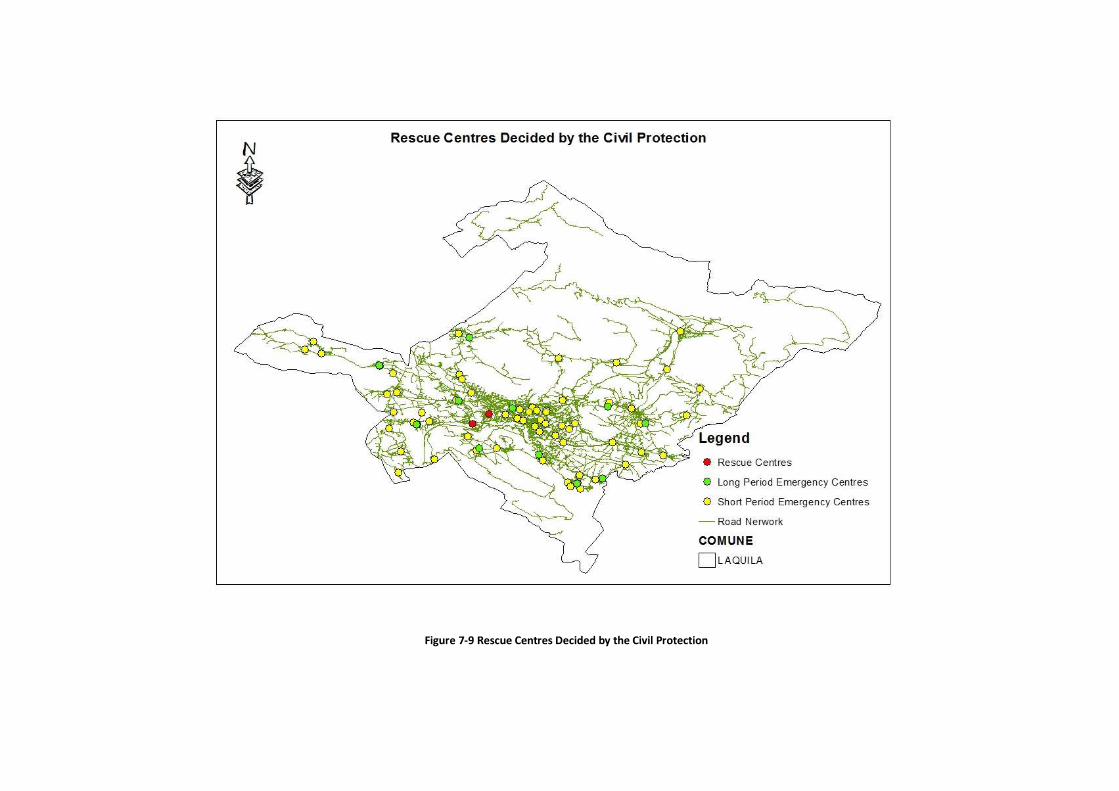
Figure 7-9 Rescue Centres Decided by the Civil Protection

111
Figure 7-10 Rescue Centes Proposed by the model

112

Chapter 8
Discussion
We have presented a method for the evacuation of urban centres to avoid human loss in
case of flooding and a method for locating rescue centres over a degraded transport
network after an earthquake. These methods, both undoubtedly need improvements and
corrections from many points of view. However, it is worth saying that this has been an
attempt to involve different disciplines so as to propose a multidisciplinary method in which
there may be the possibility of applying all competences involved. If we take advantage of
all the disciplines proposed, we may be able to produce an excellent service - product (or
on-line application) to be incorporated in comprehensive emergency management plans.
First and foremost, additional da travel costs due to the natural disaster itself have to be
better determined. As described in the relevant chapters, floods are easier to treat than
earthquakes since the phenomenon as a natural disaster is more predictable and there are
more efficient methods to calculate Vulnerability, Risk and Costs.
An efficient flood model like the one we used (CA cellular automata plain flood inundation
model) can accurately calculate the extension of a flood. If we also add all information
acquired from past events it is possible to achieve results very close to reality. In case of

114
floods, we calculated the higher possibility for road links to be blocked by the event itself
using the CA model and this is codified as da cost. It is calculated as a delay meaning that
according to the CA model, we assign very high travel costs to the road links that the model
shows are covered by water after certain periods of time (after two hours, four hours etc)
from the moment local civil protection decides to evacuate. In short terms da value is not a
delay but a probability a road link is blocked after certain periods of time. After the flood
event not all streets are available. There are still links blocked (by drifted cars, mud,
collapsed infrastructures) which are not possible to know beforehand over the whole area
of the flood. Thus, after the flood event, we can assign to da value, the cost of clearing or
repairing a link during the recovery phase of emergency management division.
In the case of an earthquake, da value is the cost of clearing or repairing links. In both cases
da value is measured in the same travel time units as link cost (time needed to cross a link
without any delay). We understand that the earthquake, as a more complicated and
unpredictable phenomenon, is more difficult to interpret and thus we are less certain about
the outcome. However, the hyperpath technique as described gives great potential to solve
earthquake problem it the future.
A deep transport study regarding the calculation of the evacuation time estimates respect
to supply and demand values, time of mobilisation and maybe human reaction. We could
consider using both pedestrian and vehicle modes to reach terminal points and maybe take
advantage of public transport.
Apart from the discussion for the effectiveness of such a system either for the earthquake or
for the flood response, we may also consider different natural disasters that may cause
similar problems. Threats today do not include only floods and earthquakes, but also
tsunamis, landslides, wildfires, tornadoes, hurricanes, pandemics, oil spills, and terrorism.
Evacuation plans have taken on greater relevance, as disasters become more and prevalent.
Both the position of rescue centres as well as the one of population centres and/or terminal
points in respect to location research presented in the third chapter can be further treated.
We take into consideration only rescue centres or terminal points decided by local civil

115
protection. However, it is important to state which nodes would represent better the
concentration of the population and refer to them as population centres. It is also very
important to consider their density and their 'capacity' at different hours of the day.
Naturally, at peak hours we would have more dense population centres than evening hours
or weekends. This should be also taken into consideration.
We can also consider population centres located in public transport stations (es bus stops-
referred to as primary population centres). Either the hyperpath concept or a* algorithm
can be selected as route choices from population centres to terminal points already decided
by local civil protection away from the crisis zone (outside the flooded area).One must
decide the capacity, period of stay and supplies for every terminal point proposed. For this
solution, public transport can be determined as the main relief instrument for pedestrians
while vehicles such as private cars may use the hyper path to arrive to a terminal point
location. In such a case, every node of the network may be referred to as a secondary
population centre and referred only to drivers located actually in the network seeking to
leave the zone in crisis. No more people should be allowed to take the car at this point and
they should only use public transport, in order to escape. Human reaction needs to be taken
into consideration as well as estimations of mobilization time and evacuation response. The
method proposed here can thus be used (rescue centre location) deploying either a* or
hyper path costs to locate places in the upper floors of buildings that would be transformed
into terminal point locations.
The proposed method to locate rescue centres can be used exactly as it is when it comes to
deal with terminal point location inside the crisis zone. This is the case when people leave
their cars and use only pedestrian mode in order to avoid any kind of congestion. Terminal
points should be locations decided by municipalities together with local civil protection
departments. These terminal points have to be in the upper floors of selected buildings, be
independent and have supplies for a long period of time. This period depends on the time
flood waters remain, keeping isolated every terminal point.

116
The hyperpath concept can be applied individuate to avoid incidents from landslides. After
long periods of rain fall we could not be sure where a landslide may occur. There are
indexes and plenty of techniques that generate the probability for a landslide to occur. We
could use the hyper path to provide risk averse guidance when local civil protection alerts
for a certain place or a certain periods are high. I understand this may vary due to
meteorological conditions.
Tsunami terminal point location could also be an idea for further research. We could use the
original rescue centre location problem and apply it to a tsunami preparedness emergency
management method. Terminal points should be high enough so as to let the waves pass
underneath their structure without being destroyed by the wave itself.

117
References
About Disasters, International Federation of Red Cross and Red Crescent Societies. (2011).
International Federation of Red Cross and Red Crescent Societies .
Advancing the Science of Climate Change. (2010). Washington, D.C.: The National Academies Press,
National Research ouncil.
Ahuja Ravindra K., Magnanti Thomas L., and Orlin James B. (1993). Network Flows: Theory,
Algorithms and Applications. Upper Saddle River, New Jersey: Prentice Hall.
Altay, N., Green III, W.G.,. (2006). OR/MS research in disaster operations management. European
Journal of Operational Research , 475-493.
America's Climate Choices. (2011). Washington, D.C.: The National Academies Press.
ANTONIOS MOURATIDIS, P. B. (2010). SRTM 300 DEM (versions 1, 2, 3, 4) validation by means of
extensivekinematic GPS measurements: a case study from North Greece. International Journal of
Remote Sensing , 6205–6222.
Arrhenius, P. S. (1896). On the Influence of Carbonic Acid in the Air upon the Temperature of the
Ground. Philosophical Magazine and journal of Science , 237-276.
ASTER GDEM Validation Team: METI/ERSDAC, NASA/LPDAAC, USGS/EROS. (2009, June). ASTER
Global DEM Validation, Summary Report.
Averbakh, I. (2003). Complexity of robust single facility location problems on networks with
uncertain edge lengths. Discrete Appl Math , 505-522.
Averbakh, I., Berman, O., . (1997). Minimax regret p-center location on a network with demand
uncertainty. Location Science , 247-254.
Averbakh, I., Berman, O.,. (2000). Algorithms for the robust 1-center problem on a tree. European
Journal of Operational Research , 292-302.
Balcik, B., Beamon, B.M., . (2008). Facility location in humanitarian relief. International Journal of
Logistics: Research and Applications , 101-121.
Balinski, M. (1965). Integer programming: Methods, uses, computation. Management Science , 253-
313.
Basoz, N. and Mander, J. (1999). Enhancement of the highway transportation lifeline module in
hazus, Final Pre-Publication Draft prepared for the National Institute of Building Sciences.
Bates, P. H. (2010). A simple inertial formulation of the shallow water equations for efficient two-
dimensional flood inundation modelling. Journal of Hydrology , 33-45.
Bell, J.E., Griffis, S.E., Cunningham, W.A., Eberlan, J.A., . (2011). Location optimization of strategic
alert sites for homeland defense. Omega-Int J Manage , 151-158.

118
Bell, M. G. (2009). Hyperstar: A multi-path Astar algorithm for risk averse vehicle navigation.
Transportation Research Part B , 97-107.
Berdica, K. (2002). An introduction to road vulnerability: what has been done, is done and should be
done. Transport Policy , 117-127.
Berkeley Earth Team. (2011). Retrieved from Berkeley Earth Surface Temperature:
http://berkeleyearth.org/
Burkard, R.E., Dollani, H.,. (2001). Robust location problems with pos/neg weights on a tree.
Networks , 102-113.
Carmen G. Rawls, , Mark A. Turnquist. (2010). Pre-positioning of emergency supplies for disaster
response. Transportation Research Part B: Methodological , 521-534.
Caunhye, A.M., Nie, X., Pokharel, S., . (Accepted Manuscript). Optimization Models in Emergency
Logistics: A Literature Review. Socio-Economic Planning Sciences .
(2011). Centre for Research on the Epidemiology of Disasters. EM-DAT The International Disaster
Database .
Chang, M.-S., Tseng, Y.-L., Chen, J.-W., . (2007). A scenario planning approach for the flood
emergency logistics preparation problem under uncertainty. 737-754: Transportation Research Part
E: Logistics and Transportation Review .
Charles S. ReVelle, Ralph W. Swain. (January 1970). Central Facilities Location. Geographical Analysis,
Volume 2, Issue 1 , 1–92.
Chen, B., Lin, C.-S.,. (1998). Minmax-regret robust 1-median location on a tree. Networks , 93-103.
Church, R.L., ReVelle, C.S., . (1974). The maximal covering location problem. Papers of the Regional
Science Association , 101-118.
Coburn, A. W., Sspence, R. J. S., Pomonis, A. (1994). Vulnerability and Risk Assessment,” Disaster
Management Training Programme (DMTP) of the United Nations Development Programme (UNDP).
Cambridge, UK: Cambridge Architectural Research Limited.
D’Ambrosio, D., Di Gregorio, S., Iovine, G. (2003). Simulating debris flows through a hexagonal
cellular automata model. Natural Hazards and Earth System Sciences , 545–559.
Database of Individual Seismogenic Sources, Instituto Nazionale di Geofisica e Vulcanologia. (2012).
Rome, Italy.
Dijkstra, E. (1959). A note on two problems in connexion with graphs. Numerische Mathematik , 269-
271.
Domschke, W., Drexl, A.,. (1985). Location and Layout Planning. An International Bibliography.
Volume 238 of Lecture Notes in Economic and Mathematical Systems, Springer-Verlag .

119
Dottori F., Todini E. (2010). Developments of a flood inundation model based on the cellular
automata approach: Testing different methods to improve model performance. Physics and
Chemistry of the Earth , 266-280.
Dottori, F., Todini, E. (2010). A 2D flood inundation model based on cellular atomata approach. XVIII
International Conference on Water Resources CMWR. Barcelona.
Feldman, E. L. ( 1966). Warehouse Location under Continuous Economies of Scale. Management
Science , 670-684.
FEMA. (2004). Hazus MH 2.0 Technical Manual. Washington, DC.: Federal Emergency Management
Agency.
Garcia-Navarro, P., Murillo, J. (2010). Finite volumes for the simulation of unsteady shallow water
flows. XVIII International Conference on Water Resources.
Garey, M. J. (1979). Computers and intractability : a guide to the theory of NP-completeness. San
Francisco.: W. H. Freeman.
Geroliminis, N., Karlaftis, M.G., Skabardonis, A., . (2009). A spatial queuing model for the emergency
vehicle districting and location problem. Transportation Research Part B: Methodological , 798-811.
Gianfranca Bellardone, Matteo Brovero, Italo Colombo, Paola Magosso, Nicoletta Negro, Cinzia
Piccioni, Carlo Troisi, Elena Turroni, Anna Ziliani. (1998). EVENTI ALLUVIONALI IN PIEMONTE. Torino:
Regione Piemonte.
Goldblatt, R. (2004). Evacuation Planning: A Key Part of Emergency Planning. Washington D.C.:
Transportation Research Board.
Green III, W. ( 2002). Four phases of emergency management. Electronic Encyclopedia of Civil
Defense and Emergency Management.
Guha-Sapir, D. V. (2011). Annual Disaster Statistical Review 2010: The Numbers and Trends. Brussels:
CRED.
Hakimi, S. (1965). Optimum distribution of switching centers in a communication network and some
related graph theoretic problems. Operations Research , 462-475.
Hakimi, S. (1964). Optimum locations of switching centers and the absolute centers and medians of a
graph. Operations Research , 450-459.
Hart, P. N. (1968). A formal basis for the heuristic determination of minimum cost paths. IEEE
Transactions on Systems Science and Cybernetics , 100-107.
Huang, R., Kim, S., Menezes, M.,. (2010). Facility location for large-scale emergencies. Annals of
Operations Research , 271-286.
IAEM. (2007). Definition, Vision, Mission, Priciples of Emergency Management. (VA): INTERNATIONAL
ASSOCIATION OF EMERGENCY MANAGERS.

120
Inc., F.-2. S. (2007). FLO-2D Users Manual. Eastern Arizona.
Ioannis, K. (2008). Reliable Dynamic In-vehicle Navigation. Centre For Transport Studies, Civil and
Enviromental Engineering. London: Imperial College London.
IPCC-INTERGOVERMANTAL PANELON CLIMATE CHANGE. (2011). Retrieved from http://www.ipcc.ch/
Jia, H. O. (2005). A modeling framework for facility location of medical services for large-scale
emergencies. IIE Transactions , 41-55.
Jia, H., Ordóñez, F., Dessouky, M.,. (2007). Solution approaches for facility location of medical
supplies for large-scale emergencies. Computers & Industrial Engineering , 257-276.
Juan de Dios Ortuzar, Luis G. Willumsen. (2001). Modelling Transport. The Atrium, Southern Gate,
Chichester, West Sussex, England: JOHN WILEY & SONS, LTD.
Kai-Uwe Eichmann, P. A. (2011). Retrieved from
http://www.espere.net/Unitedkingdom/water/uk_watexpgreenhouse.htm
Kariv, O., Hakimi, S.L., . (1979). An algorithmic approach to network location problems. SIAM Journal
on Applied Mathematics , 539-560.
Kiremidijan, A., Moore, J., Fan, Y.Y., Yazla- li, O., Basoz, N., Williams, M. . (2007). Seismic Risk
Assessment of Transportation Network Systems. Journal of Earthquake Engineering , 371-382.
Kuehn, A.A., Hamburger, M.J., . (1963). A Heuristic Program for Locating Warehouses. Management
Science , 643-666.
Luino F., A. M. (1996). Vulnerability of urban areas to flooding: events in the North-West Italy,
November 1994. Atti Sexto Congreso Nacional y Conferencia Internacional de Geologia Ambiental y
Ordenacion del Territorio, Granada, 22-25 de Abril de 1996, (pp. 309-327). Granada.
Maranzana, F. (1964). On the Location of Supply Points to Minimize Transport Costs. Operational
Research Society , 261-270.
Mason, C. (2010). Highways Agency Network Resilience and Adaptation Phase 1 Final Report.
Mendelson, E. (2009). Patent No. US 2009/0138353 Al. Coral Springs, (FL) US.
Most-Cited Authors on Climate Science. (2011). Retrieved from
http://www.eecg.utoronto.ca/~prall/climate/climate_authors_table.html
Murray-Tuite, P. (2007). A Comparison of Transportation Network Resilience under Simulated
System Optimum and User Equilibrium Conditions. IEEE , 1398 – 1405.
Neil M Hunter, Matthew S Horritt, Paul D Bates, Matthew D Wilson, Micha G F Werner. (2005). An
adaptive time step solution for raster-based storage cell modelling of floodplain inundation.
Advances in Water Resources , 975-991.
121
Nguyen, S., Pallotino, S.,. (1988). Equilibrium traffic assignment for large scale transit networks.
European Journal of Operational Research , 176-186.
Nikoofal, M.E., Sadjadi, S.J., . (2010). A robust optimization model for p-median problem with
uncertain edge lengths. THE INTERNATIONAL JOURNAL OF ADVANCED MANUFACTURING
TECHNOLOGY , 460-469.
Page, M. L. (2007, May 16). Climate change: A guide for the perplexed. Retrieved from
http://www.newscientist.com/article/dn11462-climate-change-a-guide-for-the-perplexed.html
Quarantelli, E. L. (2000). Emergencies, Disasters and Catastrophes Are Different Phenomena.
Delaware: Disaster Research Center (DRC), University of Delaware.
Reese, J. (2006). Solution methods for the p-median problem: An annotated bibliography.
NETWORKS: An International Journal , 125-142.
ReVelle, C. E. (2008). A bibliography for some fundamental problem categories in discrete location
science. European Journal of Operational Research , 817-848.
ReVelle, C.S., Eiselt, H.A., . (2005). Location analysis: A synthesis and survey - Invited review.
European Journal of Operational Research , 1-19.
Richard Church, Charles ReVelle. (1971). The Maximal Covering Location Problem. Papers of the
Regional Science Association , 101-118.
Roberto Basili, , Gianluca Valensise, Paola Vannoli, Pierfrancesco Burrato, Umberto Fracassi, Sofia
Mariano, Mara Monica Tiberti, Enzo Boschi. (2008). The Database of Individual Seismogenic Sources
(DISS), version 3: Summarizing 20 years of research on Italy's earthquake geology. Tectophysics , 20-
43.
Schiermeier, Q. (2011, February 16). Increased flood risk linked to global warming. UK: Nature.
Retrieved from http://www.nature.com/news/2011/110216/full/470316a.html
Schmöcker, J.D., Bell, M.G.H., Kurauchi, F., Shimamoto, H.,. (2009). A game theoretic approach to the
determination of hyperpaths in transportation networks. 18th International Symposium on
Transportation and Traffic Theory (ISTTT). Hong Kong: Transportation and Traffic Theory .
Serra, D. M. (1998). The p-median problem in a changing network: the case of Barcelona. Location
Science , 383-394.
Seung-Ki Min, Xuebin Zhang, Francis W. Zwiers & Gabriele C. Hegerl Human. (2011). Contribution to
more-intense precipitation extremes. (Nature, Ed.)
Shake Map Archive, Instituto Nazionale di Geofisica e Vulcanologia. (2012). Rome, Italy.
Sheu, J.-B. (23 March 2007). Challenges of emergency logistics management. Transportation
Research Part E: Logistics and Transportation Review , 655-659.

122
Snyder, L. V. (2006). Facility location under uncertainty: a review. IIE Transactions, Volume 38, Issue
7, , 547-564.
Spiess, H. F. (1989). Optimal strategies: a new assignment model for transit networks. .
Transportation Research Part B , 83-10.
Sridharan, R. (2000). The capacitated plant location problem. European Journal of Operations
Research , 203-213.
Teitz, M. B. (1968). Heuristic Methods for Estimating the Generalized Vertex Median of a Weighted
Graph. Operations Research , 955-961.
Toregas, C., Swain, R.W., ReVelle, C., Bergman, L., . (1971). The location of emergency service
facilities. Operations Research, Vol. 19, No. 6, Guidelines for the Practice of Operations Research ,
1363-1373.
Vairaktarakis, G.L., Kouvelis, P., . (March 1999). Incorporation dynamic aspects and uncertainty in 1-
median location problems. Naval Research Logistics (NRL), Volume 46, Issue 2 , 147–168.
Werner, S. C. (2006). Use of Seismic Risk Analysis of Roadway Systems to Facilitate Performance-
Based Engineering and Risk-Reduction Decision Making. REDARS.
Whitaker, R. (1981). A tight bound drop exchange algorithm for solving the p median problem.
Environment and Planning , 669-680.
William R. L. Anderegg, James W. Prall, Jacob Harold, Stephen H. Schneider. (2010). Expert Credibility
in Climate Change. PNAS Edition (Proceedings of the National Academy of Sciences of the United
States of America).
Yaghini, M. L. (2010). An Efficient Hybrid Metaheuristic for Capacitated p-Median Problem.
International Journal of Industrial Engineering & Production Research , 11-15.
Zhang, X.D., Trepanier, J.Y., Reggio, M., Camarero, R. (1994). Time-accurate local time stepping
method based on flux updating. AIAA , 1926–1929.

123
APENDIX
Introduction
There was collected an amount of valuable data for the needs of this research. All dada was
treated in a Geographic Information System (GIS). A Geographic Information system
integrates hardware, software and data for capturing, managing, analyzing and displaying all
forms of geographically referenced information.
ESRI support
For the needs of this research ESRI Italia, Italy's headquarters of the GIS software leader
worldwide, offered an one year licence of the latest GIS product of ArcGIS 10. ESRI develops
geographic Information Systems that function as an integral component in nearly every type
of organization.
Data collection
All data collected for the research developed were treated with the World Geodetic System
(WGS84) which is a standard for use in cartography, geodesy and navigation. The latest
version of the World Geodetic System, WGS84, is used by the Global Positioning System. It
is geocentric and globally consistent within one meter plus-minus.
A very valuable support for the needs of this research regarding the study of the event of
November 1994 in Alessandria Region in Piedmont (Italy) and the collection of an amazing
amount of data, was offered from Dr Fabio Luino of the Italian Research Centre, Italian
Institute for hydrological Protection, Chair of Torino CNR-IRPI data collection for Alessandria
flood. Among this important collection (see following pages) starting from the date of 1894
there were after event maps, with detailed explanations regarding, various levels of flood.
More generally we can refer to aerial photos, maps, multimedia data such as videos, and
other flood events happened at the Alessandria basin perfectly and very detailed described

124
in a report produced by Piedmont Region namely "EVENTI ALLUVIONALI IN PIEMONTE 1994-
1996".

Figure 0-1 Base maps Provided by Dr Fabio Luino CNR di Torino

126
Figure 0-2 Base maps Provided by Dr Fabio Luino CNR di Torino

Figure 0-3 Orthophoto provided by the CNR of Torino (Dr Fabio Luino)
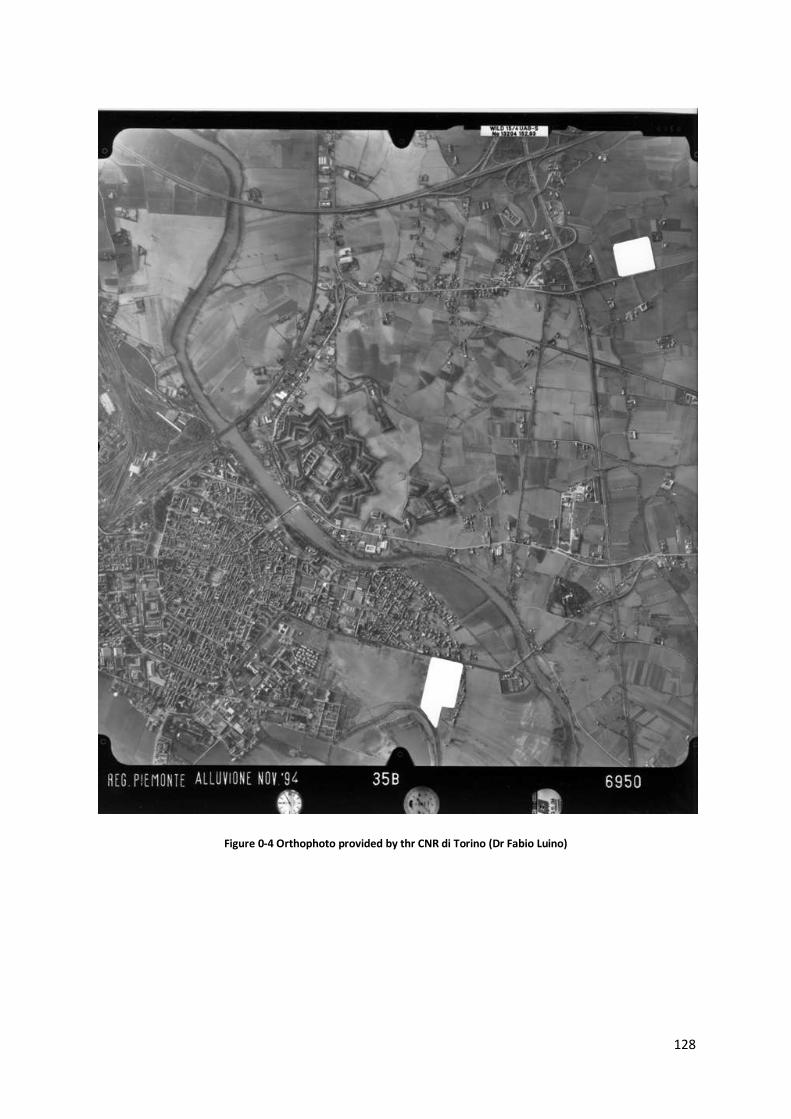
128
Figure 0-4 Orthophoto provided by thr CNR di Torino (Dr Fabio Luino)

129
We used the Tele Atlas® MultiNet® data collection kindly provided by ESRI Italia. ESRI Italia
supports Italian Research by providing data, not for commercial scope. An amazing database
of all sorts of spatial data, can also be found online and lately, it is also available in the last
versions of ArcMap.
Tele Atlas MultiNet, is the most detailed and comprehensive street network database. It is
the basis for demanding applications such as turn-by-turn route guidance, traffic
information, and others Tele Atlas is committed to constantly providing high quality maps.
All geographical data is continuously checked, upgraded and updated in the field.
Furthermore, the digital map coverage is extended every day, for the availability of other
regions, new product releases or all other information provided within the product. In the
following pages we provide visible sample of the product.

Figure 0-5 Alessandria Road Network - MultinetTM Data

131
Figure 0-6 L'Aquila Network Multinet Data

Code implementation
Both algorithms, for the calculation of all possible routes from each population centre to all
others, (hyperpaths) and for the facility location problem were implemented in MATLAB a
coding language for technical computing. MATLAB product, created from MathWorks® is a
programming environment for algorithm development, data analysis, visualization and
numerical computation. With MATLAB it is possible to solve technical computing problems
faster than with traditional programming languages such as C, C++ and Fortran. It is possible
to use MATLAB in a wide range of applications, including signal and image processing,
communications and others.
There exist several toolboxes for MATLAB. For the needs of this research we used the
Mapping Toolbox for the generation of images and shapefiles. A "shapefile" is a popular
vector data format for all Geographic Information Systems developed by ESRI. In shapefile
we can store a range of non topographical geometries and attribute information for spatial
features that can be found in a database.
Mapping Toolbox™ provides tools and utilities for analyzing geographic data and creating
map displays. You can import vector and raster data from shapefile, GeoTIFF, SDTS DEM, or
other file formats, as well as Web-based data from Web Map Service (WMS) servers. The
toolbox lets you customize the imported data by sub setting, trimming, intersecting,
adjusting spatial resolution, and applying other methods. Geographic data can be combined
with base map layers from multiple sources in a single map display. With function-level
access to all key features, it is automatically possible to create frequent tasks a geospatial
workflow.
Flood and earthquake data implementation
For the simulation of the event occurred in Alessandria in 1994, both Aster (90 meter
resolution) and SRTM (30 meter resolution) Digital Elevation Models (DEM) were collected.
The inundation model Cellular Automata of Francesco Dottori was used as described in the
sixth chapter. Francesco Dottori is part of the research group of Prof Ezio Todini, who
supervised this work.

133
Small part of the research described, (Database of Individual Seismogenic Sources, Instituto
Nazionale di Geofisica e Vulcanologia, 2012) (Shake Map Archive, Instituto Nazionale di
Geofisica e Vulcanologia, 2012) was dedicated in seismic risk assessment. For this purpose
we used information provided by the Italian, National Institute of Volcanology and
Geophysics, available online for research purposes. INGV provides a wide range of
information to researchers through their web page http://www.ingv.it/banche-dati/. We
were only referred to shakemaps and the database of Individual seismogenic sources. Apart
from that, Dr Stefano Salvi from the group of remote sensing of the National Institute of
Geophysics and Vulanology in Rome, kindly provided interferometric data. Interferometric
synthetic aperture radar, also abbreviated InSAR is a radar technique very common in
remote sensing and geodesy.
Rescue Centres - L'Aquila earthquake 6th May 2009
We report here the spaces that Civil Protection individuated to function as rescue centres or
allocation places for populations hit by an earthquake.
These are the places, where population who has been recently hit by a natural disaster such
as earthquake, or flood can find a shelter during response and recovery phases of
emergency management.
There have been individuated three types of emergency management shelters:
Short period emergency centre or attend areas (aree di attesa)
Long period emergency centre (aree di accoglienza)
Rescue centres (aree di ammassamento) where rescue vehicles are located
In the following pages we report some index cards for the places described above.

134

135

Figure 0-7 Rescue Centres along L'Aquila Municipality Network

137