modelling the effect of water depth on rock cutting ... · modelling the effect of water depth on...

Modelling The Effect of Water Depth on Rock Cutting Processes with the Use of Discrete Element Method 17

MODELLING THE EFFECT OF WATER DEPTH ON ROCK CUTTING PROCESSES WITH THE USE OF DISCRETE ELEMENT METHOD

RUDY HELMONS, SAPE ANDRIES MIEDEMA AND CEES VAN RHEE

complex compared to dry, land-based excavations due to the fact that in dredging the rock is most often cut under water. The water that is present in the pores of the rock and surrounding it can have a major influence on the rock cutting process by increasing the required cutting forces. Therefore, this paper focuses on the effects that arise due to the presence of a fluid (seawater) on the rock cutting process, especially the effect of the fluid pressure in the pores of the rock and surrounding the rock.

The basic physical phenomena that occur during rock cutting are fracturing and fragmentation of the rock due to the mechanical action of the cutting tool. The rock failure mechanism during cutting depends on many factors, especially the type of rock and rock properties, tool geometry and its position with respect to the rock. In addition, depending on the type of rock, rock properties and the conditions of the rock, distinction can be made between brittle and ductile failure. Rock chips are formed and separated due to the combined action of shear and tensile fracture, which is initiated in a crushed zone (cataclasis) near the tool tip and transmitted into the intact rock (see Figure 1).

Optimisation of the rock cutting equipment requires knowledge about the cutting process,

successful in the modelling of rock cutting processes for dry, land-based operations. In order to make the DEM useful for underwater excavations, it has been extended with a fluid coupling. The results of this extension with respect to the effect of water depth will be presented. A clear distinction between shallow water (brittle) and deep water cutting (ductile) has been observed. The newly developed method will give more insight in the physical processes that occur during cutting and it can help to improve the design and operational guidelines of the cutting equipment and processes.

INTRODUCTION

A variety of rock cutting works are carried out in dredging engineering by means of different machines and cutting tools. Whether it is for the construction of ports on new locations, the widening of canals through mountainous terrain or deep sea mining, efficient rock cutting is still one of the challenges that the dredging industry is facing. The rock cutting process for dredging purposes is even more

ABSTRACT

This paper won the IADC Young Author 2015 award and was published in the Proceedings of CEDA Dredging Days in November 2015. It is reprinted here in an adapted version with permission.

Whether it is for the construction of ports on new locations, the widening of canals through mountainous terrain or deep sea mining, efficient rock cutting is still one of the challenges that the dredging industry is facing. This gets more challenging since rock cutting in dredging is most of the time an underwater process. The water surrounding and in the pores of the rock can have a major influence on the rock cutting process by increasing the required cutting forces

During cutting, the rock matrix deforms and as a result local fluid pressure differences will occur. The magnitude of these pressure differences and its effect on the cutting process depends on the water depth and the cutting velocity. As a result, rock that is brittle under atmospheric conditions will behave more ductile in larger water depths. This paper focuses on the effect that the water depth can have on the cutting process.

The Discrete Element Method (DEM) has been

Above: Rock cutting in dredging is mostly an

underwater process. The water surrounding and in the

pores of the rock can influence the cutting process.

which can be obtained not only from experiments and field measurements, but also by simulations. The cutting process is influenced by four different groups of factors:

• Properties of rock and rock mass• Design of the cutting tool• Operational parameters such as cutting

depth, cutting speed, line spacing, etc.• Environmental parameters such as dry,

submerged, water depth, etc.All these factors influence the performance and efficiency of the cutting process.

Different models have been used to predict cutting force for a given cutting tool and rock properties. These models are based on experimental, analytical and numerical approaches. Experimental studies of rock cutting enabled better understanding of rock-tool interaction and provided information necessary for theoretical modelling. Simple analytical models have been created in attempt to describe the cutting processes. One of the earliest models is a 2D model developed by Evans (1965) for rock cutting with drag picks. In this model it is assumed that the breakage mechanism is essentially tensile and occurs along the failure surface, which approximates a circular arc. Another 2D model has been developed by Nishimatsu (1972) who assumed that failure is purely due to shear and occurs along a plane. Miedema (2014) adapted the Nishimatsu model, such that it is able to deal with tensile and shear failures. Although these rock cutting models are quite effective to predict the cutting forces, they are limited in their level of detail

on the rock cutting process.

The rock failure process during cutting can be traced in more detail by using appropriate numerical models. A number of numerical studies of rock cutting use the finite element method (FEM). However, the FEM is based on continuum mechanics theory of material modelling. Thus, the FEM has serious issues in representing the discontinuities that occur during cutting. Special formulations are necessary to introduce the possibility of dis-continuum analysis of rock fracture. In many cases, analysis of rock cutting by FEM is limited to the initial stage of major chip formation since the utilised formulation does not allow for the continuation of the analysis in the post-failure stage in which the process goes through the transition of rock mechanics to granular flow.

The discrete element method (DEM) can take into account most kinds of discontinuities and material failure characterised with multiple fractures, which makes it a suitable tool to study rock cutting. The discrete element was successfully applied to simulation of rock cutting by Huang (1999); Huang et al. (2013) and Rojek et al. (2011). A 3D DEM model of rock cutting with conical picks was developed by Su and Akcin (2011). Several attempts have been done to model the rock cutting process for (oil and/or gas) drilling. For instance, the model of Huang was used by Lei and Kaitkay (2003) to study rock cutting under a high confining pressure. Mendoza Rizo (2013) used another formulation to define the effect of a hydrostatic pressure and compared his results

with those of Lei and Kaitkay. Although the approaches of Lei and Kaitkay (2003) and Mendoza Rizo (2013) are able to mimic the rock cutting process under a high pressure, they both neglected the effects of pore pressures and fluid velocity (hydraulic conductivity).

CONFINING AND EFFECTIVE STRESSThe flow of fluid in and surrounding a rock is the main phenomenon that controls the effective stress in a rock. These mechanisms have long been recognised to cause the difference in strain-rate dependency of the rock strength for dry and saturated rock samples. Pore pressures work as a counteracting effect on the normal stress within a rock, which is expressed by Terzaghi’s law of effective stress [Terzaghi (1943)].

of the analysis in the post-failure stage in which the process goes through the transition of rock mechanics togranular flow.

The discrete element method (DEM) can take into account most kinds of discontinuities and material failurecharacterized with multiple fractures, which makes it a suitable tool to study rock cutting. The discrete elementwas successfully applied to simulation of rock cutting by Huang (1999); Huang et al. (2013) and Rojek et al.(2011). A 3D DEM model of rock cutting with conical picks was developed by Su and Akcin (2011). Severalattempts have been done to model the rock cutting process for (oil/gas) drilling. For instance, the model of Huangwas used by Lei and Kaitkay (2003) to study rock cutting under a high confining pressure. Mendoza Rizo (2013)used another formulation to define the effect of a hydrostatic pressure and compared his results with those of Leiand Kaitkay. Although the approaches of Lei and Kaitkay (2003) and Mendoza Rizo (2013) are able to mimicthe rock cutting process under a high pressure, they both neglected the effects of pore pressures and fluid velocity(hydraulic conductivity).

2 CONFINING AND EFFECTIVE STRESS

The flow of fluid in and surrounding a rock is the main phenomenon that controls the effective stress in a rock.These mechanisms have long been recognized to cause the difference in strain-rate dependency of the rock strengthfor dry and saturated rock samples. Pore pressures work as a counteracting effect on the normal stress within arock, which is expressed by Terzaghi’s law of effective stress (Terzaghi (1943)):

σ = σ′ + p (1)

with total stress σ, effective stress σ′ and pore pressure p. However, this generalization of Terzaghi’s law isonly applicable in quasi-static processes, where the local variations in pore pressure are negligible. This can beestimated with the pore Peclet number, which can be interpreted as the ratio of deformation rate over the porepressure dissipation rate. In case of rock cutting, different definitions of the pore Peclet number exist. Accordingto Detournay and Atkinson (2000), the pore Peclet number ξPe is given by

ξPe =vctc4D

=vctcnµCf

4κ(2)

with cutting velocity vc, cutting thickness tc, pore pressure diffusivity coefficient D, dynamic fluid viscosity µ,porosity n, fluid compressibility Cf and intrinsic permeability κ, in m2. According to Detournay and Atkinson(2000), three different regimes can be distinguished

• Low speed regime (0 < ξPe < 0.001): the rock responds in a drained manner during failure and ∆p � 0.

• Transient regime (0.001 < ξPe < 10): pore pressure and rock deformation are weakly coupled.

• High speed regime (ξPe > 10): pore pressure and rock deformation are strongly coupled, during failure therock responds in an undrained manner.

Detournay and Atkinson (2000) based their definitions on the application of drilling (small cutting thicknesses,in the order of mm’s or smaller). A somewhat similar definition is used by van Kesteren (1995) for dredgingpurposes (large cutting thicknesses, in the order of several to tens of cm’s). Except in these definitions, theregimes are divided in ξPe < 1, 1 < ξPe < 10 and 10 < ξPe. The difference between the defined drained andtransitional regimes is most likely due to differences in their applications, being a large difference in hydrostaticpressures (in the order of several bars for dredging applications and up to tens of MPa’s for drilling applications).

When cutting saturated rock, dilative and compactive effects occur simultaneously, which makes it difficult todistinguish these effects and their influences during cutting. In uni-axial and tri-axial tests these effects are easierto distinguish. The most profound phenomena that occur in the transient and high speed regime are:

• Compactive weakening (Swan et al. (1989))

• Dilative strengthening (often erroneously referred to as dilation hardening) (Brace and Martin III (1968),Swan et al. (1989))

Compactive weakening is related to the compression of the pore bodies in the rock. When these are beingcompressed, their volume decreases, resulting in an increase in pore pressure. This increase results in a largerpressure gradient through the rock, which ’helps’ in the deformation of the rock as an additional load, see figure 2for a schematic overview. The compactive weakening effect is also noted in single cutter tests of Zijsling (1987)on Pierre shale.

During dilation due to the creation of new and the extension of existing microcracks, the porosity of the rockincreases and the pore pressure of an effectively undrained sample locally drops. This results in an increase ofthe effective stress and thus an increase in apparent strength. A schematic overview of dilatancy strengthening isshown in figure 3.

(1)

with total stress





σ = σ′ + p (1)


ξPe =vctc4D

=vctcnµCf

4κ(2)











, effective stress





σ = σ′ + p (1)


ξPe =vctc4D

=vctcnµCf

4κ(2)











and pore pressure





σ = σ′ + p (1)


ξPe =vctc4D

=vctcnµCf

4κ(2)











. However, this generalisation of Terzaghi’s law is only applicable in quasi-static processes, where the local variations in pore pressure are negligible. This can be estimated with the pore Peclet number, which can be interpreted as the ratio of deformation rate over the pore pressure dissipation rate. In case of rock cutting, different definitions of the pore Peclet number exist. According to Detournay and Atkinson (2000), the pore Peclet number





σ = σ′ + p (1)


ξPe =vctc4D

=vctcnµCf

4κ(2)











is given by





σ = σ′ + p (1)


ξPe =vctc4D

=vctcnµCf

4κ(2)











(2)

with cutting velocity





σ = σ′ + p (1)


ξPe =vctc4D

=vctcnµCf

4κ(2)











, cutting thickness





σ = σ′ + p (1)


ξPe =vctc4D

=vctcnµCf

4κ(2)











, pore pressure diffusivity coefficient





σ = σ′ + p (1)


ξPe =vctc4D

=vctcnµCf

4κ(2)











, dynamic fluid viscosity





σ = σ′ + p (1)


ξPe =vctc4D

=vctcnµCf

4κ(2)











, porosity





σ = σ′ + p (1)


ξPe =vctc4D

=vctcnµCf

4κ(2)











, fluid compressibility





σ = σ′ + p (1)


ξPe =vctc4D

=vctcnµCf

4κ(2)











and intrinsic permeability





σ = σ′ + p (1)


ξPe =vctc4D

=vctcnµCf

4κ(2)











, in





σ = σ′ + p (1)


ξPe =vctc4D

=vctcnµCf

4κ(2)











. According to Detournay and Atkinson (2000), three different regimes can be distinguished

• Low speed regime





σ = σ′ + p (1)


ξPe =vctc4D

=vctcnµCf

4κ(2)











: the rock responds in a drained manner during failure and





σ = σ′ + p (1)


ξPe =vctc4D

=vctcnµCf

4κ(2)











.• Transient regime





σ = σ′ + p (1)


ξPe =vctc4D

=vctcnµCf

4κ(2)











: pore pressure and rock deformation are weakly coupled.

• High speed regime





σ = σ′ + p (1)


ξPe =vctc4D

=vctcnµCf

4κ(2)











: pore pressure and rock deformation are strongly coupled, during failure the rock responds in an undrained manner.

18 Terra et Aqua | Number 142 | March 2016

Figure 1. Phenomenological

model of rock cutting

process, based on van

Kesteren (1995)

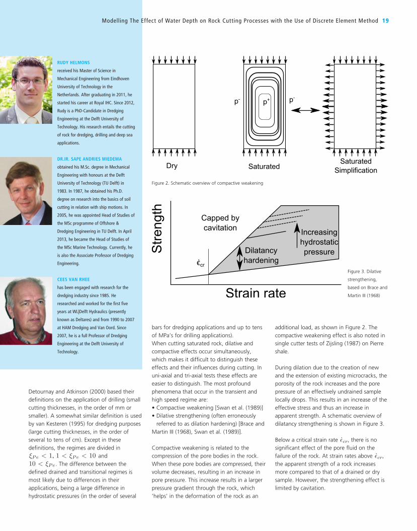
Detournay and Atkinson (2000) based their definitions on the application of drilling (small cutting thicknesses, in the order of mm or smaller). A somewhat similar definition is used by van Kesteren (1995) for dredging purposes (large cutting thicknesses, in the order of several to tens of cm). Except in these definitions, the regimes are divided in





σ = σ′ + p (1)


ξPe =vctc4D

=vctcnµCf

4κ(2)











and





σ = σ′ + p (1)


ξPe =vctc4D

=vctcnµCf

4κ(2)











. The difference between the defined drained and transitional regimes is most likely due to differences in their applications, being a large difference in hydrostatic pressures (in the order of several

RUDY HELMONS

received his Master of Science in

Mechanical Engineering from Eindhoven

University of Technology in the

Netherlands. After graduating in 2011, he

started his career at Royal IHC. Since 2012,

Rudy is a PhD-Candidate in Dredging

Engineering at the Delft University of

Technology. His research entails the cutting

of rock for dredging, drilling and deep sea

applications.

DR.IR. SAPE ANDRIES MIEDEMA

obtained his M.Sc. degree in Mechanical

Engineering with honours at the Delft

University of Technology (TU Delft) in

1983. In 1987, he obtained his Ph.D.

degree on research into the basics of soil

cutting in relation with ship motions. In

2005, he was appointed Head of Studies of

the MSc programme of Offshore &

Dredging Engineering in TU Delft. In April

2013, he became the Head of Studies of

the MSc Marine Technology. Currently, he

is also the Associate Professor of Dredging

Engineering.

CEES VAN RHEE

has been engaged with research for the

dredging industry since 1985. He

researched and worked for the first five

years at WL|Delft Hydraulics (presently

known as Deltares) and from 1990 to 2007

at HAM Dredging and Van Oord. Since

2007, he is a full Professor of Dredging

Engineering at the Delft University of

Technology.

bars for dredging applications and up to tens of MPa’s for drilling applications).When cutting saturated rock, dilative and compactive effects occur simultaneously, which makes it difficult to distinguish these effects and their influences during cutting. In uni-axial and tri-axial tests these effects are easier to distinguish. The most profound phenomena that occur in the transient and high speed regime are:• Compactive weakening [Swan et al. (1989)]• Dilative strengthening (often erroneously

referred to as dilation hardening) [Brace andMartin III (1968), Swan et al. (1989)].

Compactive weakening is related to the compression of the pore bodies in the rock. When these pore bodies are compressed, their volume decreases, resulting in an increase in pore pressure. This increase results in a larger pressure gradient through the rock, which ’helps’ in the deformation of the rock as an

additional load, as shown in Figure 2. The compactive weakening effect is also noted in single cutter tests of Zijsling (1987) on Pierre shale.

During dilation due to the creation of new and the extension of existing microcracks, the porosity of the rock increases and the pore pressure of an effectively undrained sample locally drops. This results in an increase of the effective stress and thus an increase in apparent strength. A schematic overview of dilatancy strengthening is shown in Figure 3.

Below a critical strain rate

Dry SaturatedSaturated

Simplification

p+p- p-

Figure 2. Schematic overview of compactive weakening

Strain rate

Stre

ngth

Capped by cavitation Increasing

hydrostatic pressureDilatancy

hardeningϵcr

Figure 3. Dilative strengthening, based on Brace and Martin III (1968)

Below a critical strain rate ε̇cr, there is no significant effect of the pore fluid on the failure of the rock. At strainrates above ε̇cr, the apparent strength of a rock increases more compared to that of a drained or dry sample.However, the strengthening effect is limited by cavitation.

In case of cavitation, the pressure in the dilative zone drops below the vapour pressure of the fluid, causing thepore fluid to evaporate. As a result the pressure in the pores can hardly drop and the bulk compressibility of thefluid increases several orders of magnitude. As a result, ∆p is limited. The maximum achievable ∆p, and thusthe maximum dilative strengthening, increases linearly with the hydrostatic pressure.

3 METHOD

3.1 RockIn DEM, the solid material is represented as a collection of particles (these can be any arbitrarily shape, most oftenspheres in 3D or discs with unit thickness in 2D are used for the sake of simplicity) that have mutual interactionsin normal and tangential directions. This paper gives the description and results in 2D. The translational androtational motion of a particle is governed by the standard equations of rigid body mechanics

mi�ai = �Fi (3)

Ii�αi = �Ti (4)

�F and �T are the sums of all forces and moments applied to the particle i due to external loading, contact inter-actions with neighboring objects and from damping in the system. Due to the high computational effort that isneeded to calculate the forces acting on the particles, the equations of are integrated with an explicit multi-steptime integration scheme, i.e. the velocity Verlet scheme.

�rn+1i = �rni + �vni ∆t+

1

2�ani ∆t2 (5)

�vn+1/2i = �vni +

1

2�ani ∆t (6)

�an+1i =

1

mi

∑�Fn+1i (7)

�vn+1i = �v

i+1/2i +

1

2�an+1i ∆t (8)

, there is no significant effect of the pore fluid on the failure of the rock. At strain rates above


Simplification

p+p- p-


Strain rate

Stre

ngth



hardeningϵcr




3 METHOD


mi�ai = �Fi (3)




1

2�ani ∆t2 (5)

�vn+1/2i = �vni +

1

2�ani ∆t (6)

�an+1i =

1

mi

∑�Fn+1i (7)

�vn+1i = �v

i+1/2i +

1

2�an+1i ∆t (8)

, the apparent strength of a rock increases more compared to that of a drained or dry sample. However, the strengthening effect is limited by cavitation.



Figure 3. Dilative

strengthening,

based on Brace and

Martin III (1968)


Simplification

p+p- p-

Strain rate

Stre

ngth



hardeningϵcr

In case of cavitation, the pressure in the dilative zone drops below the vapour pressure of the fluid, causing the pore fluid to evaporate. As a result, the pressure in the pores can hardly drop and the bulk compressibility of the fluid increases several orders of magnitude. As a result, is limited. The maximum achievable , and thus the maximum dilative strengthening, increases linearly with the hydrostatic pressure.

METHODRockIn DEM, the solid material is represented as a collection of particles (these particles can be in any arbitrary shape; for the sake of simplicity , most often spheres in 3D or discs with unit thickness in 2D are used) that have mutual interactions in normal and tangential directions. This paper gives the description and results in 2D. The translational and rotational motion of a particle is governed by the standard equations of rigid body mechanics


Simplification

p+p- p-


Strain rate

Stre

ngth



hardeningϵcr




3 METHOD


mi�ai = �Fi (3)




1

2�ani ∆t2 (5)

�vn+1/2i = �vni +

1

2�ani ∆t (6)

�an+1i =

1

mi

∑�Fn+1i (7)

�vn+1i = �v

i+1/2i +

1

2�an+1i ∆t (8)

(3) (4)


Simplification

p+p- p-


Strain rate

Stre

ngth



hardeningϵcr




3 METHOD


mi�ai = �Fi (3)




1

2�ani ∆t2 (5)

�vn+1/2i = �vni +

1

2�ani ∆t (6)

�an+1i =

1

mi

∑�Fn+1i (7)

�vn+1i = �v

i+1/2i +

1

2�an+1i ∆t (8)

and


Simplification

p+p- p-


Strain rate

Stre

ngth



hardeningϵcr




3 METHOD


mi�ai = �Fi (3)




1

2�ani ∆t2 (5)

�vn+1/2i = �vni +

1

2�ani ∆t (6)

�an+1i =

1

mi

∑�Fn+1i (7)

�vn+1i = �v

i+1/2i +

1

2�an+1i ∆t (8)

are the sums of all forces and moments applied to the particle

originally developed by Lucy (1977). DEM and SP work in a co-located fashion, meaning that both methods usethe same discretisation points.

In the DEM-SP model, the discretized particles are taken from a particle size distribution and randomly stackedtogether. The unstructured positions and random size (and thus mass) of the particles can easily result innumerical instabilities and inaccuracies. To adjust for the random size and positioning of the particles, theCorrective Smoothed Particle Approach (CSPM) is used (Chen et al. (1999)).

In CSPM, the kernel interpolation of a field quantity A (which can be any arbitrary parameter) is calculated by

A (�ri) =

∑j AjmjW (�ri − �rj , h)∑j mjW (�ri − �rj , h)

(15)

with particle mass m, kernel function W , position r, smoothing length h, index i for particle under considerationand index j for neighboring particles (including particle i). In a similar fashion, the first order derivative of afunction A is determined by

∇iA (�ri) =

∑j (Ai −Aj)mj∇W (�ri − �rj , h)∑j (�ri − �rj)mj∇W (�ri − �rj , h)

(16)

where ∇i is the gradient with respect to particle i. Higher order derivatives cannot be calculated directly. Thefirst derivative is necessary to determine the volumetric strain rate in equation (3.2),

ε̇v = ∇ · �v =∂vx∂x

+∂vy∂y

(17)

Here the Wendland C2 kernel function is used Wendland (1995)

W =

{7π2 (1−R)

4(4R+ 1) if R ≤ 1

0 if R > 1(18)

where

R =||�ri − �rj ||

h(19)

To calculate the diffusive term in (3.2), we make use of the results of Cleary and Monaghan (1999):

∇ · κ∇p =∑j

mj (κi + κj)

ρi(pi − pj)

�nij · ∇W (�ri − �rj , h)

||�ri − �rj ||(20)

where �nij is the normal unit vector of the neighboring particle centers. Note that here κ is a property of theparticles and thus that it can differ throughout the rock sample. In our case, it is assumed that κ is constant.

Two way coupling is applied every timestep. DEM is advanced half a timestep, based on the intermediate velocitiesthe volumetric strain rate is calculated with SP. This is then used to advance the pore pressure diffusion onetimestep in a forward Euler scheme. The local pressure gradient of the fluid is calculated based on the new porepressure distribution. The pressure gradient is then added as an interaction force to the sum of forces acting on theparticles through

�F = −∇pπd2p4

w (21)

with particle diameter dp and unit thickness w. Finally the DEM is advanced the second half timestep. See figure5 for the flowchart of this coupling scheme.It is possible that the fluid pressure drops below the vapour pressure during simulations. When this happens, theliquid will vaporize. As a result, the compressibility of the fluid of increases with several orders of magnitude.In the simulations, this is modeled through a simplified approach. When the pressure drops below the pressureminimum, the pressure value is fixed at the minimum pressure. From thereon it is only possible to increase thepressure by having fluid flow towards the cavitated zone, so if

pi < pmin then pi = pmin and∂pi∂t

= max

(∂pi∂t

, 0

)(22)

due to external loading, contact interactions with neighbouring objects and from damping in the system. Due to the high computational effort that is needed to calculate the forces acting on the particles, the equations of are integrated with an explicit multi-step time integration scheme, i.e. the velocity Verlet scheme.


Simplification

p+p- p-


Strain rate

Stre

ngth



hardeningϵcr




3 METHOD


mi�ai = �Fi (3)




1

2�ani ∆t2 (5)

�vn+1/2i = �vni +

1

2�ani ∆t (6)

�an+1i =

1

mi

∑�Fn+1i (7)

�vn+1i = �v

i+1/2i +

1

2�an+1i ∆t (8)

It needs mentioning that It needs mentioning that �Fn+1 is actually a function of �rn+1 and �vn+1/2. Because of the use of an explicitscheme, there is a limitation on the size of the timestep to ensure a stable solution, meaning ∆t ≤ ∆tcr. ∆tcr isapproximated by the highest of natural frequencies of a contact pair.

The interaction force between a pair of particles can either consist of a collision type or a bond type of interaction.In both cases the force is composed of normal and tangential components, with

�F = �Fn + �Ft = �nFn + �tFt (9)

where �n is the unit vector normal to the particle surface at the point of interaction. The contact forces Fn andFt are determined with a constitutive model for the interaction. At the beginning of each simulation, a bondis installed between neighboring particles. These bonds are defined by a linear elastic perfect brittle model(see figure 4), meaning that a bond breaks immediately when its strength is exceeded. Note that a bond canbreak either in normal (tension) or in tangential (shear) direction and not in compressive direction (macroscopiccompressive failure is considered as a localization of many micro-shear and tensile failures). After a bond isbroken, the bond will be removed from the simulation. Besides bonds, there are also collisional interactions. Inthese interactions the normal force is only active in compressive direction and the tangential force can be eitherstatic or dynamic friction.

Figure 4. Linear elastic perfect brittle bond model: (left) normal direction, (middle) shear direction with contact after failure and (right) sheardirection without contact after failure

To reach a quasi-static equilibirum, it is necessary that the kinetic energy dissipates. Especially since the DEMis a highly dynamics approach, damping is required. This is done by application of numerical damping, as inPotyondy and Cundall (2004) and is often used in DEM-applications for rock. The damping force is in the formof

�Fd = −αd||∑

�F ||sign(�v) (10)

with damping coefficient αd.The DEM can be regarded as a micromechanical model, with the contact and bond model parameters beingmicroparameters. It is assumed that with the adequate micromechanical parameters macroscopic rock propertiesare obtained, of which the Young’s modulus E, Poisson ratio ν, and compressive and tensile strengths σc andσt are the most relevant. These properties will be used in calibrating the micromechanical model to sufficientlymimic the macroscopic rock mechanics.

3.2 Fluid pressureThe effect of a rapidly changing effective stress is modeled with the use of a pore pressure diffusion equation, asin Coussy (2004). This equation is based on the combination of mass conservation, Darcy flow and a constitutiveequation for the compressibility of the pore fluid, given respectively by

Dζ

Dt+∇ · �u = 0 (11)

�u = −κ

µ∇p (12)

p = M (ζ − αεv) (13)

which through substitution results in the pore pressure diffusion equation given by

Dp

Dt−M∇ ·

(κ

µ∇p

)= −αM

DεvDt

(14)

with pressure p, fluid bulk modulus M , intrinsic permeability κ, dynamic fluid viscosity µ, effective stresscoefficient α and volumetric strain εv .

The coupling of the discrete data obtained from the DEM computations with the pore pressure diffusion equation(3.2) is obtained by using a Smoothed Particle (SP) approach. SP is a kernel interpolation technique that is

is actually a function of It needs mentioning that �Fn+1 is actually a function of �rn+1 and �vn+1/2. Because of the use of an explicit

scheme, there is a limitation on the size of the timestep to ensure a stable solution, meaning ∆t ≤ ∆tcr. ∆tcr isapproximated by the highest of natural frequencies of a contact pair.


�F = �Fn + �Ft = �nFn + �tFt (9)




�Fd = −αd||∑

�F ||sign(�v) (10)



Dζ

Dt+∇ · �u = 0 (11)

�u = −κ

µ∇p (12)

p = M (ζ − αεv) (13)


Dp

Dt−M∇ ·

(κ

µ∇p

)= −αM

DεvDt

(14)



and It needs mentioning that �Fn+1 is actually a function of �rn+1 and �vn+1/2. Because of the use of an explicitscheme, there is a limitation on the size of the timestep to ensure a stable solution, meaning ∆t ≤ ∆tcr. ∆tcr isapproximated by the highest of natural frequencies of a contact pair.


�F = �Fn + �Ft = �nFn + �tFt (9)




�Fd = −αd||∑

�F ||sign(�v) (10)



Dζ

Dt+∇ · �u = 0 (11)

�u = −κ

µ∇p (12)

p = M (ζ − αεv) (13)


Dp

Dt−M∇ ·

(κ

µ∇p

)= −αM

DεvDt

(14)



. Because of the use of an explicit scheme, there is a limitation on the size of the timestep to ensure a stable solution, meaning It needs mentioning that �Fn+1 is actually a function of �rn+1 and �vn+1/2. Because of the use of an explicit

scheme, there is a limitation on the size of the timestep to ensure a stable solution, meaning ∆t ≤ ∆tcr. ∆tcr isapproximated by the highest of natural frequencies of a contact pair.


�F = �Fn + �Ft = �nFn + �tFt (9)




�Fd = −αd||∑

�F ||sign(�v) (10)



Dζ

Dt+∇ · �u = 0 (11)

�u = −κ

µ∇p (12)

p = M (ζ − αεv) (13)


Dp

Dt−M∇ ·

(κ

µ∇p

)= −αM

DεvDt

(14)



is approximated by the highest of natural frequencies of a contact pair.

The interaction force between a pair of particles can either consist of a collision type or a bond type of interaction. In both cases the force is composed of normal and tangential components, with

It needs mentioning that �Fn+1 is actually a function of �rn+1 and �vn+1/2. Because of the use of an explicitscheme, there is a limitation on the size of the timestep to ensure a stable solution, meaning ∆t ≤ ∆tcr. ∆tcr isapproximated by the highest of natural frequencies of a contact pair.


�F = �Fn + �Ft = �nFn + �tFt (9)




�Fd = −αd||∑

�F ||sign(�v) (10)



Dζ

Dt+∇ · �u = 0 (11)

�u = −κ

µ∇p (12)

p = M (ζ − αεv) (13)


Dp

Dt−M∇ ·

(κ

µ∇p

)= −αM

DεvDt

(14)



(9)

where



�F = �Fn + �Ft = �nFn + �tFt (9)




�Fd = −αd||∑

�F ||sign(�v) (10)



Dζ

Dt+∇ · �u = 0 (11)

�u = −κ

µ∇p (12)

p = M (ζ − αεv) (13)


Dp

Dt−M∇ ·

(κ

µ∇p

)= −αM

DεvDt

(14)



is the unit vector normal to the particle surface at the point of interaction and



�F = �Fn + �Ft = �nFn + �tFt (9)




�Fd = −αd||∑

�F ||sign(�v) (10)



Dζ

Dt+∇ · �u = 0 (11)

�u = −κ

µ∇p (12)

p = M (ζ − αεv) (13)


Dp

Dt−M∇ ·

(κ

µ∇p

)= −αM

DεvDt

(14)



is perpendicular to



�F = �Fn + �Ft = �nFn + �tFt (9)




�Fd = −αd||∑

�F ||sign(�v) (10)



Dζ

Dt+∇ · �u = 0 (11)

�u = −κ

µ∇p (12)

p = M (ζ − αεv) (13)


Dp

Dt−M∇ ·

(κ

µ∇p

)= −αM

DεvDt

(14)



. The contact forces



�F = �Fn + �Ft = �nFn + �tFt (9)




�Fd = −αd||∑

�F ||sign(�v) (10)



Dζ

Dt+∇ · �u = 0 (11)

�u = −κ

µ∇p (12)

p = M (ζ − αεv) (13)


Dp

Dt−M∇ ·

(κ

µ∇p

)= −αM

DεvDt

(14)



and



�F = �Fn + �Ft = �nFn + �tFt (9)




�Fd = −αd||∑

�F ||sign(�v) (10)



Dζ

Dt+∇ · �u = 0 (11)

�u = −κ

µ∇p (12)

p = M (ζ − αεv) (13)


Dp

Dt−M∇ ·

(κ

µ∇p

)= −αM

DεvDt

(14)



are determined with a constitutive model for the interaction. At the beginning of each simulation, a bond is installed between neighbouring particles. These bonds are defined by a linear elastic perfect brittle model (see Figure 4), meaning that a bond breaks immediately when its strength is exceeded. Note that a bond can break either in normal (tension) or in tangential (shear) direction and not in compressive direction (macroscopic compressive failure is considered as a localisation of many micro-shear and tensile failures). After a bond is broken, the bond will be removed from the simulation. Besides bonds, there are also collisional interactions. In these interactions the normal force is only active in a compressive direction and the tangential force can be either static or dynamic friction.

To reach a quasi-static equilibrium, it is necessary that the kinetic energy dissipates. Especially since the DEM is a highly dynamic approach, damping is required. This is done by application of numerical damping, as ni Potyondy and Cundall (2004) and is often used in DEM-applications for rock. The damping force is in the form of



�F = �Fn + �Ft = �nFn + �tFt (9)




�Fd = −αd||∑

�F ||sign(�v) (10)



Dζ

Dt+∇ · �u = 0 (11)

�u = −κ

µ∇p (12)

p = M (ζ − αεv) (13)


Dp

Dt−M∇ ·

(κ

µ∇p

)= −αM

DεvDt

(14)



(10)

with damping coefficient



�F = �Fn + �Ft = �nFn + �tFt (9)




�Fd = −αd||∑

�F ||sign(�v) (10)



Dζ

Dt+∇ · �u = 0 (11)

�u = −κ

µ∇p (12)

p = M (ζ − αεv) (13)


Dp

Dt−M∇ ·

(κ

µ∇p

)= −αM

DεvDt

(14)



.

The DEM can be regarded as a micro mechanical

model, with the contact and bond model parameters being microparameters. It is assumed that with the adequate micro-mechanical parameters macroscopic rock properties are obtained, of which the Young’s modulus



�F = �Fn + �Ft = �nFn + �tFt (9)




�Fd = −αd||∑

�F ||sign(�v) (10)



Dζ

Dt+∇ · �u = 0 (11)

�u = −κ

µ∇p (12)

p = M (ζ − αεv) (13)


Dp

Dt−M∇ ·

(κ

µ∇p

)= −αM

DεvDt

(14)



, Poisson ratio



�F = �Fn + �Ft = �nFn + �tFt (9)




�Fd = −αd||∑

�F ||sign(�v) (10)



Dζ

Dt+∇ · �u = 0 (11)

�u = −κ

µ∇p (12)

p = M (ζ − αεv) (13)


Dp

Dt−M∇ ·

(κ

µ∇p

)= −αM

DεvDt

(14)



, and compressive and tensile strengths



�F = �Fn + �Ft = �nFn + �tFt (9)




�Fd = −αd||∑

�F ||sign(�v) (10)



Dζ

Dt+∇ · �u = 0 (11)

�u = −κ

µ∇p (12)

p = M (ζ − αεv) (13)


Dp

Dt−M∇ ·

(κ

µ∇p

)= −αM

DεvDt

(14)



and



�F = �Fn + �Ft = �nFn + �tFt (9)




�Fd = −αd||∑

�F ||sign(�v) (10)



Dζ

Dt+∇ · �u = 0 (11)

�u = −κ

µ∇p (12)

p = M (ζ − αεv) (13)


Dp

Dt−M∇ ·

(κ

µ∇p

)= −αM

DεvDt

(14)



are the most relevant. These properties will be used in calibrating the micromechanical model to sufficiently mimic the macroscopic rock mechanics. Fluid PressureThe effect of a rapidly changing effective stress is modelled with the use of a pore pressure diffusion equation, as in Coussy (2004). This equation is based on the combination of mass conservation, Darcy flow and a constitutive equation for the compressibility of the pore fluid, given respectively by



�F = �Fn + �Ft = �nFn + �tFt (9)




�Fd = −αd||∑

�F ||sign(�v) (10)



Dζ

Dt+∇ · �u = 0 (11)

�u = −κ

µ∇p (12)

p = M (ζ − αεv) (13)


Dp

Dt−M∇ ·

(κ

µ∇p

)= −αM

DεvDt

(14)



(11)

(12)



�F = �Fn + �Ft = �nFn + �tFt (9)




�Fd = −αd||∑

�F ||sign(�v) (10)



Dζ

Dt+∇ · �u = 0 (11)

�u = −κ

µ∇p (12)

p = M (ζ − αεv) (13)


Dp

Dt−M∇ ·

(κ

µ∇p

)= −αM

DεvDt

(14)





�F = �Fn + �Ft = �nFn + �tFt (9)




�Fd = −αd||∑

�F ||sign(�v) (10)



Dζ

Dt+∇ · �u = 0 (11)

�u = −κ

µ∇p (12)

p = M (ζ − αεv) (13)


Dp

Dt−M∇ ·

(κ

µ∇p

)= −αM

DεvDt

(14)



(13)




�F = �Fn + �Ft = �nFn + �tFt (9)




�Fd = −αd||∑

�F ||sign(�v) (10)



Dζ

Dt+∇ · �u = 0 (11)

�u = −κ

µ∇p (12)

p = M (ζ − αεv) (13)


Dp

Dt−M∇ ·

(κ

µ∇p

)= −αM

DεvDt

(14)



(14)

with pressure



�F = �Fn + �Ft = �nFn + �tFt (9)




�Fd = −αd||∑

�F ||sign(�v) (10)



Dζ

Dt+∇ · �u = 0 (11)

�u = −κ

µ∇p (12)

p = M (ζ − αεv) (13)


Dp

Dt−M∇ ·

(κ

µ∇p

)= −αM

DεvDt

(14)



, fluid bulk modulus



�F = �Fn + �Ft = �nFn + �tFt (9)




�Fd = −αd||∑

�F ||sign(�v) (10)



Dζ

Dt+∇ · �u = 0 (11)

�u = −κ

µ∇p (12)

p = M (ζ − αεv) (13)


Dp

Dt−M∇ ·

(κ

µ∇p

)= −αM

DεvDt

(14)



, intrinsic permeability



�F = �Fn + �Ft = �nFn + �tFt (9)




�Fd = −αd||∑

�F ||sign(�v) (10)



Dζ

Dt+∇ · �u = 0 (11)

�u = −κ

µ∇p (12)

p = M (ζ − αεv) (13)


Dp

Dt−M∇ ·

(κ

µ∇p

)= −αM

DεvDt

(14)



, dynamic fluid viscosity



�F = �Fn + �Ft = �nFn + �tFt (9)




�Fd = −αd||∑

�F ||sign(�v) (10)



Dζ

Dt+∇ · �u = 0 (11)

�u = −κ

µ∇p (12)

p = M (ζ − αεv) (13)


Dp

Dt−M∇ ·

(κ

µ∇p

)= −αM

DεvDt

(14)



, effective stress coefficient



�F = �Fn + �Ft = �nFn + �tFt (9)




�Fd = −αd||∑

�F ||sign(�v) (10)



Dζ

Dt+∇ · �u = 0 (11)

�u = −κ

µ∇p (12)

p = M (ζ − αεv) (13)


Dp

Dt−M∇ ·

(κ

µ∇p

)= −αM

DεvDt

(14)



and volumetric strain



�F = �Fn + �Ft = �nFn + �tFt (9)




�Fd = −αd||∑

�F ||sign(�v) (10)



Dζ

Dt+∇ · �u = 0 (11)

�u = −κ

µ∇p (12)

p = M (ζ − αεv) (13)


Dp

Dt−M∇ ·

(κ

µ∇p

)= −αM

DεvDt

(14)



.The coupling of the discrete data obtained from the DEM computations with the pore pressure diffusion equation (14) is obtained by using a Smoothed Particle (SP) approach. SP is a kernel interpolation technique that is

Figure 4. Linear elastic perfect brittle bond model: (left) normal direction, (middle) shear direction with contact after

failure and (right) shear direction without contact after failure

(5)

(6)

(7)

(8)



originally developed by Lucy (1977). DEM and SP work in a co-located fashion, meaning that both methods use the same discretisation points.

In the DEM-SP model, the discretized particles are taken from a particle size distribution and randomly stacked together. The unstructured positions and random size (and thus mass) of the particles can easily result in numerical instabilities and inaccuracies. To adjust for the random size and positioning of the particles, the Corrective Smoothed Particle Approach (CSPM) is used [Chen et al. (1999)].

In CSPM, the kernel interpolation of a field quantity




A (�ri) =


(15)


∇iA (�ri) =


(16)


ε̇v = ∇ · �v =∂vx∂x

+∂vy∂y

(17)


W =

{7π2 (1−R)

4(4R+ 1) if R ≤ 1

0 if R > 1(18)

where

R =||�ri − �rj ||

h(19)


∇ · κ∇p =∑j

mj (κi + κj)

ρi(pi − pj)

�nij · ∇W (�ri − �rj , h)

||�ri − �rj ||(20)



�F = −∇pπd2p4

w (21)



= max

(∂pi∂t

, 0

)(22)

(which can be any arbitrary parameter) is calculated by




A (�ri) =


(15)


∇iA (�ri) =


(16)


ε̇v = ∇ · �v =∂vx∂x

+∂vy∂y

(17)


W =

{7π2 (1−R)

4(4R+ 1) if R ≤ 1

0 if R > 1(18)

where

R =||�ri − �rj ||

h(19)


∇ · κ∇p =∑j

mj (κi + κj)

ρi(pi − pj)

�nij · ∇W (�ri − �rj , h)

||�ri − �rj ||(20)



�F = −∇pπd2p4

w (21)



= max

(∂pi∂t

, 0

)(22)

(15)

with particle mass




A (�ri) =


(15)


∇iA (�ri) =


(16)


ε̇v = ∇ · �v =∂vx∂x

+∂vy∂y

(17)


W =

{7π2 (1−R)

4(4R+ 1) if R ≤ 1

0 if R > 1(18)

where

R =||�ri − �rj ||

h(19)


∇ · κ∇p =∑j

mj (κi + κj)

ρi(pi − pj)

�nij · ∇W (�ri − �rj , h)

||�ri − �rj ||(20)



�F = −∇pπd2p4

w (21)



= max

(∂pi∂t

, 0

)(22)

, kernel function




A (�ri) =


(15)


∇iA (�ri) =


(16)


ε̇v = ∇ · �v =∂vx∂x

+∂vy∂y

(17)


W =

{7π2 (1−R)

4(4R+ 1) if R ≤ 1

0 if R > 1(18)

where

R =||�ri − �rj ||

h(19)


∇ · κ∇p =∑j

mj (κi + κj)

ρi(pi − pj)

�nij · ∇W (�ri − �rj , h)

||�ri − �rj ||(20)



�F = −∇pπd2p4

w (21)



= max

(∂pi∂t

, 0

)(22)

, position




A (�ri) =


(15)


∇iA (�ri) =


(16)


ε̇v = ∇ · �v =∂vx∂x

+∂vy∂y

(17)


W =

{7π2 (1−R)

4(4R+ 1) if R ≤ 1

0 if R > 1(18)

where

R =||�ri − �rj ||

h(19)


∇ · κ∇p =∑j

mj (κi + κj)

ρi(pi − pj)

�nij · ∇W (�ri − �rj , h)

||�ri − �rj ||(20)



�F = −∇pπd2p4

w (21)



= max

(∂pi∂t

, 0

)(22)

, smoothing length




A (�ri) =


(15)


∇iA (�ri) =


(16)


ε̇v = ∇ · �v =∂vx∂x

+∂vy∂y

(17)


W =

{7π2 (1−R)

4(4R+ 1) if R ≤ 1

0 if R > 1(18)

where

R =||�ri − �rj ||

h(19)


∇ · κ∇p =∑j

mj (κi + κj)

ρi(pi − pj)

�nij · ∇W (�ri − �rj , h)

||�ri − �rj ||(20)



�F = −∇pπd2p4

w (21)



= max

(∂pi∂t

, 0

)(22)

, index




A (�ri) =


(15)


∇iA (�ri) =


(16)


ε̇v = ∇ · �v =∂vx∂x

+∂vy∂y

(17)


W =

{7π2 (1−R)

4(4R+ 1) if R ≤ 1

0 if R > 1(18)

where

R =||�ri − �rj ||

h(19)


∇ · κ∇p =∑j

mj (κi + κj)

ρi(pi − pj)

�nij · ∇W (�ri − �rj , h)

||�ri − �rj ||(20)



�F = −∇pπd2p4

w (21)



= max

(∂pi∂t

, 0

)(22)

for particle under consideration and index




A (�ri) =


(15)


∇iA (�ri) =


(16)


ε̇v = ∇ · �v =∂vx∂x

+∂vy∂y

(17)


W =

{7π2 (1−R)

4(4R+ 1) if R ≤ 1

0 if R > 1(18)

where

R =||�ri − �rj ||

h(19)


∇ · κ∇p =∑j

mj (κi + κj)

ρi(pi − pj)

�nij · ∇W (�ri − �rj , h)

||�ri − �rj ||(20)



�F = −∇pπd2p4

w (21)



= max

(∂pi∂t

, 0

)(22)

for neighboring particles (including particle




A (�ri) =


(15)


∇iA (�ri) =


(16)


ε̇v = ∇ · �v =∂vx∂x

+∂vy∂y

(17)


W =

{7π2 (1−R)

4(4R+ 1) if R ≤ 1

0 if R > 1(18)

where

R =||�ri − �rj ||

h(19)


∇ · κ∇p =∑j

mj (κi + κj)

ρi(pi − pj)

�nij · ∇W (�ri − �rj , h)

||�ri − �rj ||(20)



�F = −∇pπd2p4

w (21)



= max

(∂pi∂t

, 0

)(22)

). In a similar fashion, the first order derivative of a function




A (�ri) =


(15)


∇iA (�ri) =


(16)


ε̇v = ∇ · �v =∂vx∂x

+∂vy∂y

(17)


W =

{7π2 (1−R)

4(4R+ 1) if R ≤ 1

0 if R > 1(18)

where

R =||�ri − �rj ||

h(19)


∇ · κ∇p =∑j

mj (κi + κj)

ρi(pi − pj)

�nij · ∇W (�ri − �rj , h)

||�ri − �rj ||(20)



�F = −∇pπd2p4

w (21)



= max

(∂pi∂t

, 0

)(22)

is determined by




A (�ri) =


(15)


∇iA (�ri) =


(16)


ε̇v = ∇ · �v =∂vx∂x

+∂vy∂y

(17)


W =

{7π2 (1−R)

4(4R+ 1) if R ≤ 1

0 if R > 1(18)

where

R =||�ri − �rj ||

h(19)


∇ · κ∇p =∑j

mj (κi + κj)

ρi(pi − pj)

�nij · ∇W (�ri − �rj , h)

||�ri − �rj ||(20)



�F = −∇pπd2p4

w (21)



= max

(∂pi∂t

, 0

)(22)

(16)

where




A (�ri) =


(15)


∇iA (�ri) =


(16)


ε̇v = ∇ · �v =∂vx∂x

+∂vy∂y

(17)


W =

{7π2 (1−R)

4(4R+ 1) if R ≤ 1

0 if R > 1(18)

where

R =||�ri − �rj ||

h(19)


∇ · κ∇p =∑j

mj (κi + κj)

ρi(pi − pj)

�nij · ∇W (�ri − �rj , h)

||�ri − �rj ||(20)



�F = −∇pπd2p4

w (21)



= max

(∂pi∂t

, 0

)(22)

is the gradient with respect to particle




A (�ri) =


(15)


∇iA (�ri) =


(16)


ε̇v = ∇ · �v =∂vx∂x

+∂vy∂y

(17)


W =

{7π2 (1−R)

4(4R+ 1) if R ≤ 1

0 if R > 1(18)

where

R =||�ri − �rj ||

h(19)


∇ · κ∇p =∑j

mj (κi + κj)

ρi(pi − pj)

�nij · ∇W (�ri − �rj , h)

||�ri − �rj ||(20)



�F = −∇pπd2p4

w (21)



= max

(∂pi∂t

, 0

)(22)

. Higher order derivatives cannot be calculated directly. The first derivative is necessary to determine the volumetric strain rate in equation (14).




A (�ri) =


(15)


∇iA (�ri) =


(16)


ε̇v = ∇ · �v =∂vx∂x

+∂vy∂y

(17)


W =

{7π2 (1−R)

4(4R+ 1) if R ≤ 1

0 if R > 1(18)

where

R =||�ri − �rj ||

h(19)


∇ · κ∇p =∑j

mj (κi + κj)

ρi(pi − pj)

�nij · ∇W (�ri − �rj , h)

||�ri − �rj ||(20)



�F = −∇pπd2p4

w (21)



= max

(∂pi∂t

, 0

)(22)

(17)





A (�ri) =


(15)


∇iA (�ri) =


(16)


ε̇v = ∇ · �v =∂vx∂x

+∂vy∂y

(17)


W =

{7π2 (1−R)

4(4R+ 1) if R ≤ 1

0 if R > 1(18)

where

R =||�ri − �rj ||

h(19)


∇ · κ∇p =∑j

mj (κi + κj)

ρi(pi − pj)

�nij · ∇W (�ri − �rj , h)

||�ri − �rj ||(20)



�F = −∇pπd2p4

w (21)



= max

(∂pi∂t

, 0

)(22)

(18) where




A (�ri) =


(15)


∇iA (�ri) =


(16)


ε̇v = ∇ · �v =∂vx∂x

+∂vy∂y

(17)


W =

{7π2 (1−R)

4(4R+ 1) if R ≤ 1

0 if R > 1(18)

where

R =||�ri − �rj ||

h(19)


∇ · κ∇p =∑j

mj (κi + κj)

ρi(pi − pj)

�nij · ∇W (�ri − �rj , h)

||�ri − �rj ||(20)



�F = −∇pπd2p4

w (21)



= max

(∂pi∂t

, 0

)(22)

(19)

To calculate the diffusive term in (14), we make use of the results of Cleary and Monaghan (1999):




A (�ri) =


(15)


∇iA (�ri) =


(16)


ε̇v = ∇ · �v =∂vx∂x

+∂vy∂y

(17)


W =

{7π2 (1−R)

4(4R+ 1) if R ≤ 1

0 if R > 1(18)

where

R =||�ri − �rj ||

h(19)


∇ · κ∇p =∑j

mj (κi + κj)

ρi(pi − pj)

�nij · ∇W (�ri − �rj , h)

||�ri − �rj ||(20)



�F = −∇pπd2p4

w (21)



= max

(∂pi∂t

, 0

)(22)

(20) where




A (�ri) =


(15)


∇iA (�ri) =


(16)


ε̇v = ∇ · �v =∂vx∂x

+∂vy∂y

(17)


W =

{7π2 (1−R)

4(4R+ 1) if R ≤ 1

0 if R > 1(18)

where

R =||�ri − �rj ||

h(19)


∇ · κ∇p =∑j

mj (κi + κj)

ρi(pi − pj)

�nij · ∇W (�ri − �rj , h)

||�ri − �rj ||(20)



�F = −∇pπd2p4

w (21)



= max

(∂pi∂t

, 0

)(22)

is the normal unit vector of the neighbouring particle centres. Note that here



�F = �Fn + �Ft = �nFn + �tFt (9)




�Fd = −αd||∑

�F ||sign(�v) (10)



Dζ

Dt+∇ · �u = 0 (11)

�u = −κ

µ∇p (12)

p = M (ζ − αεv) (13)


Dp

Dt−M∇ ·

(κ

µ∇p

)= −αM

DεvDt

(14)



is a property of the particles and thus that it can differ throughout the rock sample. In our case, it is assumed that



�F = �Fn + �Ft = �nFn + �tFt (9)




�Fd = −αd||∑

�F ||sign(�v) (10)



Dζ

Dt+∇ · �u = 0 (11)

�u = −κ

µ∇p (12)

p = M (ζ − αεv) (13)


Dp

Dt−M∇ ·

(κ

µ∇p

)= −αM

DεvDt

(14)



is constant.Two way coupling is applied every timestep. DEM is advanced half a timestep, based on the intermediate velocities the volumetric strain rate is calculated with SP. This is then used to advance the pore pressure diffusion one timestep in a forward Euler scheme. The local pressure gradient of the fluid is calculated based on the new pore pressure distribution. The pressure gradient is then added as an interaction force to the sum of forces acting on the particles through




A (�ri) =


(15)


∇iA (�ri) =


(16)


ε̇v = ∇ · �v =∂vx∂x

+∂vy∂y

(17)


W =

{7π2 (1−R)

4(4R+ 1) if R ≤ 1

0 if R > 1(18)

where

R =||�ri − �rj ||

h(19)


∇ · κ∇p =∑j

mj (κi + κj)

ρi(pi − pj)

�nij · ∇W (�ri − �rj , h)

||�ri − �rj ||(20)



�F = −∇pπd2p4

w (21)



= max

(∂pi∂t

, 0

)(22)

(21)

with particle diameter




A (�ri) =


(15)


∇iA (�ri) =


(16)


ε̇v = ∇ · �v =∂vx∂x

+∂vy∂y

(17)


W =

{7π2 (1−R)

4(4R+ 1) if R ≤ 1

0 if R > 1(18)

where

R =||�ri − �rj ||

h(19)


∇ · κ∇p =∑j

mj (κi + κj)

ρi(pi − pj)

�nij · ∇W (�ri − �rj , h)

||�ri − �rj ||(20)



�F = −∇pπd2p4

w (21)



= max

(∂pi∂t

, 0

)(22)

and unit thickness




A (�ri) =


(15)


∇iA (�ri) =


(16)


ε̇v = ∇ · �v =∂vx∂x

+∂vy∂y

(17)


W =

{7π2 (1−R)

4(4R+ 1) if R ≤ 1

0 if R > 1(18)

where

R =||�ri − �rj ||

h(19)


∇ · κ∇p =∑j

mj (κi + κj)

ρi(pi − pj)

�nij · ∇W (�ri − �rj , h)

||�ri − �rj ||(20)



�F = −∇pπd2p4

w (21)



= max

(∂pi∂t

, 0

)(22)

. Finally the DEM is advanced the second half timestep. See figure 5 for the flowchart of this coupling scheme.It is possible that the fluid pressure drops below the vapour pressure during simulations. When this happens, the liquid will vaporise. As a result, the compressibility of the fluid of increases with several orders of magnitude. In the simulations, this is modelled through a simplified approach. When the pressure drops

below the pressure minimum, the pressure value is fixed at the minimum pressure. From thereon it is only possible to increase the pressure by having fluid flow towards the cavitated zone, so if




A (�ri) =


(15)


∇iA (�ri) =


(16)


ε̇v = ∇ · �v =∂vx∂x

+∂vy∂y

(17)


W =

{7π2 (1−R)

4(4R+ 1) if R ≤ 1

0 if R > 1(18)

where

R =||�ri − �rj ||

h(19)


∇ · κ∇p =∑j

mj (κi + κj)

ρi(pi − pj)

�nij · ∇W (�ri − �rj , h)

||�ri − �rj ||(20)



�F = −∇pπd2p4

w (21)



= max

(∂pi∂t

, 0

)(22)

then




A (�ri) =


(15)


∇iA (�ri) =


(16)


ε̇v = ∇ · �v =∂vx∂x

+∂vy∂y

(17)


W =

{7π2 (1−R)

4(4R+ 1) if R ≤ 1

0 if R > 1(18)

where

R =||�ri − �rj ||

h(19)


∇ · κ∇p =∑j

mj (κi + κj)

ρi(pi − pj)

�nij · ∇W (�ri − �rj , h)

||�ri − �rj ||(20)



�F = −∇pπd2p4

w (21)



= max

(∂pi∂t

, 0

)(22) and




A (�ri) =


(15)


∇iA (�ri) =


(16)


ε̇v = ∇ · �v =∂vx∂x

+∂vy∂y

(17)


W =

{7π2 (1−R)

4(4R+ 1) if R ≤ 1

0 if R > 1(18)

where

R =||�ri − �rj ||

h(19)


∇ · κ∇p =∑j

mj (κi + κj)

ρi(pi − pj)

�nij · ∇W (�ri − �rj , h)

||�ri − �rj ||(20)



�F = −∇pπd2p4

w (21)



= max

(∂pi∂t

, 0

)(22)

(22)

Boundary ConditionsIn DEM-SP, boundary conditions have to be applied for both the rock and fluid phase. In the case of rock this is done by restricting or prescribing the motion of specific particles or walls. In case of the fluid pressure, the boundary conditions are somewhat harder to set. The SP discretisation of (14) in itself automatically applies Neumann boundary condition (zero gradient), meaning that it allows no fluid flow across the boundaries of the rock. This is applicable in the case where equipment is moving through the rock (cutting teeth, compressive tests, splitting tests, etc.). In case of a rock boundary that is in contact with clear fluid, such as the top layer of the seabed, a Dirichlet boundary condition (fixed value, such as hydrostatic pressure) is applied. However, the boundaries of the rock may change during the simulation. Therefore, it is necessary to use a method to determine what particles are part of the rock boundary. To determine this, we make use of the divergence of position, as suggested by Muhammad et al. (2013).

Calculate ∑ = , , ∇ ()

Calculate , , ∇ (SPH)

Neighbour detection (Staged, DEM/SPH)

Calculate , / (DEM)

START

Calculate , (DEM)

FINISH

→ + 1

Figure 5. Flowchart of the DEM-SP method

3.3 Boundary conditionsIn DEM-SP, boundary conditions have to be applied for both the rock and fluid phase. For rock this is done byrestricting or prescribing the motion of specific particles or walls. In case of the fluid pressure, the boundaryconditions are somewhat harder to set. The SP discretisation of (3.2) in itself automatically applies Neumannboundary condition (zero gradient), meaning that it allows no fluid flow across the boundaries of the rock. Thisis applicable in the case where equipment is moving through the rock (cutting teeth, compressive tests, splittingtests, etc.). In case of a rock boundary that is in contact with clear fluid, like the top layer of the seabed, a Dirichletboundary condition (fixed value, such as hydrostatic pressure) is applied. However, the boundaries of the rockmay change during the simulation. Therefore it is necessary to use a method to determine what particles are partof the rock boundary. To determine this, we make use of the divergence of position, as suggested by Muhammadet al. (2013).

∇ · �r =∂x

∂x+

∂y

∂y= 2 (23)

This is applied to the standard Smoothed Particle approach of Lucy (1977), because otherwise the CSPM inequation (3.2) automatically corrects for the particle deficiency, always setting at a value of 2.

∇iA (�ri) =∑j

mjAj

ρj∇W (�ri − �rj , h) (24)

In the interior domain of the rock, equation (3.3) is valid. However, at the boundaries this value differs due toparticle deficiency, see figure 6. Here, particles with ∇ · �r ≤ 1.5 are considered to be part of the boundary. Withthis technique, the particles that require a Dirichlet boundary condition can now be identified.

4 RESULTS

The input and output parameters of the simulated rock are shown in table 1. For this paper, the parameters werechosen to represent a weak sandstone with a relatively high permeability.

A set of cutting simulations has been performed with varying water depth. Simulations have run at depths of 0,10, 40, 100, 250, 1000 and 2000 meters. All other parameters have been kept constant. The larger water depthsare simulated to investigate what differences there might be between dredging (< 30 m) and deep sea miningapplications. In these simulations, rock is cut with a chisel at a 60 deg angle, a cutting depth of 0.02 meter, acutting velocity of 1 m/s. Furthermore, it is assumed that the pore pressure is initially equal to the hydrostaticpressure. These conditions are chosen to cover both dredging and deep sea mining applications. Although thecutting velocity and the cutting depth are smaller than often used for dredging purposes, here it is chosen to do itat lower values for academic purposes.

(23)

This is applied to the standard SP approach of Lucy (1977), because otherwise the CSPM in equation (16) automatically corrects for the particle deficiency, always setting at a value of 2.




Calculate , / (DEM)

START

Calculate , (DEM)

FINISH

→ + 1



∇ · �r =∂x

∂x+

∂y

∂y= 2 (23)


∇iA (�ri) =∑j

mjAj

ρj∇W (�ri − �rj , h) (24)


4 RESULTS



(24) In the interior domain of the rock, equation (23) is valid. However, at the boundaries this value differs due to particle deficiency as can be seen in Figure 6. Here, particles with




Calculate , / (DEM)

START

Calculate , (DEM)

FINISH

→ + 1



∇ · �r =∂x

∂x+

∂y

∂y= 2 (23)


∇iA (�ri) =∑j

mjAj

ρj∇W (�ri − �rj , h) (24)


4 RESULTS



are considered to be part of the boundary. With this technique, the particles Figure 5. Flowchart of the DEM-SP method




Calculate , / (DEM)

START

Calculate , (DEM)

FINISH

→ + 1

Calc

ulat

e ∑

=

, ,∇

(

)

Calc

ulat

e ,

,∇ (S

PH)

Nei

ghbo

ur d

etec

tion

(Sta

ged,

DEM

/SPH

)

Calc

ulat

e

,/

(DEM

)

STAR

T

Calc

ulat

e

, (D

EM)

FIN

ISH

→+

1

that require a Dirichlet boundary condition can now be identified.

RESULTSThe input and output parameters of the simulated rock are shown in Table 1. For this paper, the parameters were chosen to represent a weak sandstone with a relatively high permeability.

A set of cutting simulations were performed with varying water depths. These simulations were run at depths of 0, 10, 40, 100, 250, 1000 and 2000 m. All other parameters were kept constant. The larger water depths were simulated to investigate the differences that might be between dredging (< 30 m) and deep sea mining applications. In these simulations, rock was cut with a chisel at a 60 degree angle, a cutting depth of 0.02 m, a cutting velocity of 1 m/s. Furthermore, it was assumed that the pore pressure is initially equal to the hydrostatic pressure. These conditions were chosen to cover both dredging and deep sea mining applications. Although the cutting velocity and the cutting depth were smaller than what are often used for dredging purposes, for academic purposes, lower values were chosen for the simulations.

The resulting averaged cutting forces are shown in Figure 8 (see next page). Note that the vertical force was directed such that the tool had to be pushed into the rock (downwards). In some areas where the average pore pressure was calculated – the locations of these areas are shown in Figure 7

and they moved along with the movement of the chisel. The averaged results of these pressure measurements are shown in Figures 9 and 10, here referred to as P1 , P2 and P3 . All nodes cover the same size, an area of 2.5 mm in width and height. Node 1 was located exactly at the tool tip, node 2 was 12.5 mm in front and 10 mm above the tool tip and node 3 was 30 mm in front of the tool tip. The position of the nodes were kept the same for all simulations.

Different types of behaviour were noted – at shallow water depths the cutting process was dominated by tensile failures (see Figure 11) whereas for deep sea applications, the rock cutting process was dominated by shear failures (see Figure 12).

DISCUSSIONA clear distinction was observed between low and high hydrostatic pressures. At low hydrostatic pressures, the cutting process was dominated by the occurrence of large chips. Those chips occur when the cutting process is

dominated by tensile failures. At high hydrostatic pressures, the cutting process was dominated by shear failures. Chips still seemed to occur in hyperbaric conditions, but these were significantly smaller, as can be seen in Figures 11 and 12. The transition between the two regimes is at a water depth of 300 m, based on the operating conditions as in Table 1.

The vertical cutting force was also significantly lower than the horizontal force, which did not correspond to what was derived from previous experiments. Such an effect was also noted in the DEM-simulations of dry rock cutting by Rojek et al. (2011). They noted that the vertical cutting force in 2D is strongly underestimated, while in 3D simulations this

force is in the same range as in practice. Rojek et al. (2011) argue that this difference is caused by the lack of geometric information in 2D simulations, which seems valid considering that the 2D simulations are an approximation of plane strain.

At several points relative to the tool, the average pore pressures were measured. The averaged pore pressure at the tip of the chisel (P1) shows no dependence on the hydrostatic pressure. This corresponds with the effective stress theory, initially the pore and hydrostatic pressures are in equilibrium and in the crushed zone, the deformation is always dominated by compression, leading to an increased pore pressure.

The averaged pore pressure measurements in


Table 1. Input and output parameters of simulated rock

Figure 6. Schematic overview of particle deficiency

Figure 7. Locations of the averaged pressure nodes.

The nodes move with the cutting tool

∇ · �r = 2∇ · �r < 2



Model input Model output GeometryKn 10 GPa UCS 13.8 MPa Block height 0.1 mKs 25 GPa BTS 2.55 MPa Block width 0.2 mTn 10 kNm-1 E 5.5 GPa Cutting depth 0.02 mTs 20 kNm-1 ν 0.22 Tool angle 60 degµgrain 1 Tool width 0.02 mR 0.0002− 0.0004 mm Water depth 0− 2000 mα 0.5 Cutting velocity 1 m/sκ 1 · 10−14m2

n 0.18ρgrain 2800 kgm-3

h 0.0015 mM 2 GPaµfluid 0.001 Pas

The resulting averaged cutting forces are shown in figure 8. Note that the vertical force is directed such that thetool has to be pushed into the rock (downwards). In some areas, the average pore pressure is calculated, thelocations of these areas are shown in figure 7 and move along with the movement of the chisel. The averagedresults of these pressure measurements are shown in figures 9 and 10, here referred to as P1, P2 and P3. All nodescover the same size, an area of 2.5 mm in width and height. Node 1 is located exactly at the tool tip, node 2 is12.5 mm in front and 10 mm above the tool tip and node 3 is 30 mm in front of the tool tip. The position of thenodes is kept the same for all simulations.

1 23

y+

x+

Figure 7. Locations of the averaged pressure nodes. The nodes move with the cutting tool

1 23

y+

x+

∇ · �r = 2∇ · �r < 2







1 23

y+

x+


∇ · �r = 2∇ · �r < 2







1 23

y+

x+


front of the chisel (P2, P3) both showed a transition from a pressure increase to a pressure drop (see Figure 10). This can be explained as that the rock deformation is dominated by compression in shallow water depths and that it is dominated by dilation at large water depths. The positive averaged pressure difference noted in shallow waters was caused by the brittle behaviour of the cutting process. Before a chip can occur, the tool first needs to build up pressure to reach a stress condition where the rock starts to fail by the occurrence of macro-cracks. However, the exact location of these cracks always differed and they are often outside the pressure averaging areas. In that sense, the average pressure measured at P4 and P4 is often that of the pore pressure in an ’intact’ chip. At large water depths, the rock failure is dominated by shear failures, resulting in dilation. As a result, the pressure dropped in

the dilative zone and the fluid had to flow towards it. In these water depths, the rock cutting process seems similar compared with the cutting of sand [which is also noted by Miedema and Zijsling (2012)].

ACKNOWLEDGEMENTSThe research is part of the PhD-project of EXHADERO (Excavation of Hard Deposits and Rock), which was performed with support of Delft University of Technology, Agentschap NL, Royal Dutch Shell, Royal Boskalis Westminster, Van Oord Dredging and Marine Contractors and Royal IHC. The authors are grateful for their support.

Modelling The Effect of Water Depth on Rock Cutting Processes with the Use of Discrete Element Method 23105 106 1070

1

2

·104

ph [Pa]

F̄c[N

]

F̄c (ph)

Fc,x

Fc,y

105 106 1070

0.5

1

1.5·107

ph [Pa]

p1−ph[P

a]

∆p at tip of tool

105 106 107−1

−0.5

0

·107

ph [Pa]

ph−p2,3[P

a]

∆p in front of tool

ph − p2ph − p3

Different types of behavior are noted, for shallow water depths the cutting process is dominated by tensile failures(see figure 11), for deep sea applications, the rock cutting process is dominated by shear failures (see figure 12).

5 DISCUSSION

A clear distinction is observed between low and high hydrostatic pressures. At low hydrostatic pressures, thecutting process is dominated by the occurrence of large chips. Those chips occur when the cutting process is dom-inated by tensile failures. At high hydrostatic pressures, the cutting process is dominated by shear failures. Chipsstill seem to occur in hyperbaric conditions, but these are significantly smaller, as can be seen in figures 11 and 12.The transition between the two regimes is at a water depth of 300 m, based on the operating conditions as in table 1.

Also notice that the vertical cutting force is significantly lower than the horizontal force, which does notcorrespond with experience from experiments. Such an effect is also noted in the DEM-simulations of dry rockcutting by Rojek et al. (2011). They noted that the vertical cutting force in 2D is strongly underestimated, whilein 3D simulations this force is in the same range as in practice. Rojek et al. (2011) argue that this differenceis caused by the lack of geometric information in 2D simulations, which seems valid considering that the 2Dsimulations are an approximation of plane strain.

At several points relative to the tool, the average pore pressures have been measured. The averaged porepressure at the tip of the chisel (P1) shows no dependence on the hydrostatic pressure. This corresponds with theeffective stress theory, initially the pore and hydrostatic pressures are in equilibrium and in the crushed zone, thedeformation is always dominated by compression, leading to an increased pore pressure.

105 106 1070

1

2

·104

ph [Pa]

F̄c[N

]

F̄c (ph)

Fc,x

Fc,y

105 106 1070

0.5

1

1.5·107

ph [Pa]p1−ph[P

a]

∆p at tip of tool

105 106 107−1

−0.5

0

·107

ph [Pa]

ph−p2,3[P

a]


ph − p2ph − p3


5 DISCUSSION




105 106 1070

1

2

·104

ph [Pa]

F̄c[N

]

F̄c (ph)

Fc,x

Fc,y

105 106 1070

0.5

1

1.5·107

ph [Pa]

p1−

ph[P

a]

∆p at tip of tool

105 106 107−1

−0.5

0

·107

ph [Pa]

ph−

p2,3[P

a]


ph − p2ph − p3


5 DISCUSSION




Figure 8. Cutting force vs hydrostatic pressure Figure 9. Averaged pressure difference in node 1 vs

hydrostatic pressure, based on operating conditions as

in Table 1

Figure 10. Averaged pressure difference in nodes 2 and

3 vs hydrostatic pressure, based on operating conditions

as in Table 1

Figure 12. Damage during cutting at 2000 m water depth. Damage is defined as

Figure 11. Damage during cutting at 0 m water depth. Damage is defined as D = 1− # bonds# initial bonds


The averaged pore pressure measurements in front of the chisel (P2, P3) both show a transition from a pressureincrease to a pressure drop (see figure 10). This can be explained as that the the rock deformation is dominatedby compression in shallow water depths and that it is dominated by dilation at large water depths. The fact thata positive averaged pressure difference is noted in shallow waters is caused by the brittle behavior of the cuttingprocess. Before a chip can occur, the tool first needs to build up pressure to reach a stress condition where therock starts to fail by the occurrence of macro-cracks. However, the exact location of these cracks always differsand those are often outside the pressure averaging areas. In that sense, the average pressure measured at P4 andP4 is often that of the pore pressure in an ’intact’ chip. At large water depths, the rock failure is dominated byshear failures, resulting in dilation. As a result, the pressure drops in the dilative zone and the fluid has to flowtowards it. In these water depths, the rock cutting process seems similar compared with the cutting of sand (whichis also noted by Miedema and Zijsling (2012)).

6 CONCLUSION

The DEM has been often used to simulate rock cutting processes of dry rock. An extension of DEM with SPto model the pore pressure effects gives promising results concerning the cutting of saturated rock. Two cuttingregimes can be distinguished relative to the water depth, the tensile failure dominated regime for shallow waterdepths and the shear failure dominated regime for large water depths.

Figure 11. Damage during cutting at 0 m water depth. Damage is defined as



The averaged pore pressure measurements in front of the chisel (P2, P3) both show a transition from a pressureincrease to a pressure drop (see figure 10). This can be explained as that the the rock deformation is dominatedby compression in shallow water depths and that it is dominated by dilation at large water depths. The fact thata positive averaged pressure difference is noted in shallow waters is caused by the brittle behavior of the cuttingprocess. Before a chip can occur, the tool first needs to build up pressure to reach a stress condition where therock starts to fail by the occurrence of macro-cracks. However, the exact location of these cracks always differsand those are often outside the pressure averaging areas. In that sense, the average pressure measured at P4 andP4 is often that of the pore pressure in an ’intact’ chip. At large water depths, the rock failure is dominated byshear failures, resulting in dilation. As a result, the pressure drops in the dilative zone and the fluid has to flowtowards it. In these water depths, the rock cutting process seems similar compared with the cutting of sand (whichis also noted by Miedema and Zijsling (2012)).

6 CONCLUSION

The DEM has been often used to simulate rock cutting processes of dry rock. An extension of DEM with SPto model the pore pressure effects gives promising results concerning the cutting of saturated rock. Two cuttingregimes can be distinguished relative to the water depth, the tensile failure dominated regime for shallow waterdepths and the shear failure dominated regime for large water depths.

CONCLUSIONS The DEM has often been used to simulate rock cutting processes of dry rock. An extension of DEM with SP to model the pore pressure effects gives promising results concerning the cutting of saturated rock. Two cutting regimes can be distinguished relative to the water depth, the tensile failure dominated regime for shallow water depths and the shear failure dominated regime for large water depths. Though the results of the method correspond with observations in experiments and literature, more quantitative validation will be needed. This will be done in future work by comparing the simulations with cone indention tests, rock cutting tests and (oil/gas) drilling tests.

Lucy, L. (1977). A numerical approach to the

testing of the fission hypothesis. Astronomical

Journal, 1013–1024.

Mendoza Rizo, J. (2013). Considerations for

discrete element modeling of rock cutting.

Doctoral, University of Pittsburgh.

Miedema, S. (2014). The delft sand, clay &

rock cutting model. Amsterdam, the

Netherlands: IOS Press.

Miedema, S. A. and D. Zijsling (2012).

Hyperbaric rock cutting. In OMAE 2012, Rio

de Janeiro, Brazil.

Muhammad, N., B. D. Rogers, and L. Li (2013,

March). Understanding the behaviour of

pulsed laser dry and wet micromachining

processes by multi-phase smoothed particle

hydrodynamics (SPH) modelling. Journal of

Physics D: Applied Physics 46(9), 095101.

Nishimatsu, Y. (1972). The mechanics of rock

cutting. International Journal of Rock

Mechanics and Mining Sciences 9, 261–270.

Potyondy, D. and P. Cundall (2004,

December). A bonded-particle model for rock.

International Journal of Rock Mechanics and

Mining Sciences 41(8), 1329–1364.

Rojek, J., E. Onate, C. Labra, and H. Kargl

(2011, September). Discrete element

simulation of rock cutting. International

Journal of Rock Mechanics and Mining

Sciences 48(6), 996–1010.

Su, O. and N. A. Akcin (2011). Numerical

simulation of rock cutting using the discrete

element method. International Journal of Rock

Mechanics and Mining Sciences 48(3), 434–

442.

Swan, G., J. Cook, S. Bruce, and R. Meehan

(1989, March). Strain rate effects in

Kimmeridge bay shale. International Journal of

Rock Mechanics and Mining Sciences &

Geomechanics Abstracts 26(2), 135–149.

Terzaghi, K. (1943). Theoretical Soil

Mechanics. John Wiley and Sons.

van Kesteren, W. G. M. (1995). Numerical

simulations of crack bifurcation in the chip

forming cutting process in rock. Fracture of

Brittle Disordered Materials: concrete, Rock

and Ceramics 26(1-2), 21–25.

Wendland (1995). Piecewise polynomial

positive definite and compactly supported

radial functions of minimal degree. Advances

in Computational Mathematics 4, 389–396.

Zijsling, D. (1987). Single cutter testing - A key

for PDC bit development. In Offshore Europe

87, Aberdeen, UK, pp. SPE16529/1.


REFERENCES

Brace, W. and R. Martin III (1968). A test of

the law of effective stress for crystalline rocks

of low porosity. International Journal of Rock

Mechanics and Mining Sciences 5, 415–426.

Chen, J. K., J. E. Beraun, and T. C. Carney

(1999). A corrective smoothed particle

method for boundary value problems in heat

conduction. International Journal for

Numerical Methods in Engineering 252 (June

1998), 231-252.

Cleary, P. W. and J. J. Monaghan (1999,

January). Conduction modelling using

Smoothed Particle Hydrodynamics. Journal of

Computational Physics 148(1), 227–264.

Coussy, P. O. (2004). Poromechanics. West

Sussex: John Wiley & Sons Ltd.

Detournay, E. and C. Atkinson (2000,

October). Influence of pore pressure on the

drilling response in low-permeability shear-

dilatant rocks. International Journal of Rock

Mechanics and Mining Sciences 37(7), 1091–

1101.

Evans, I. (1965, March). The force required to

cut coal with blunt wedges. International

Journal of Rock Mechanics and Mining

Sciences & Geomechanics Abstracts 2(1), 1–12.

Huang, H. (1999). Discrete element modeling

of tool-rock interaction. Doctoral, University of

Minnesota.

Huang, H., B. Lecampion, and E. Detournay

(2013). Discrete element modeling of tool-

rock interaction I : rock cutting. International

Journal for Numerical and Analytical Methods

in Geomechanics 37(13), 1913–1929.

Lei, S. and P. Kaitkay (2003). Distinct Element

Modeling of Rock Cutting under Hydrostatic

Pressure. Key Engineering Materials 250, 110–

117.

modelling the effect of water depth on rock cutting ... · modelling the effect of water depth on...

Documents