modelling plant variation through growth - algorithmic...

Modelling Plant Variation Through GrowthLisa Streit, Pavol Federl, Mario Costa SousaDepartment of Computer Science, University of Calgaryemail: streitl|federl|[email protected]

AbstractThis paper introduces a method for creating naturally varied plants from a given basic plantmodel. Previous techniques create variation in plants by introducing local randomness to theplant model's description. However, randomness is restricted by the model's parameterizationand lack of correlation between local features making varying global properties (e.g. branchand stem curvature) difficult. We present a biologically−based method which mimics theunderpinnings of variation in real plants. This method uses a feedback control system tosimulate the biological growth mechanism by which a plant naturally responds toenvironmental factors. We show that our technique creates more realistically varied modelsby modelling growth responses to stimuli, and provides a method for quickly creatingnumerous similar models, none of which are exactly alike.

ReferenceL. Streit, P. Federl, and M.C. Sousa: Modelling Plant Variation Through Growth. In Computer GraphicsForum 24 (3), pp. 497−506, 2005.

EUROGRAPHICS 2005 / M. Alexa and J. Marks(Guest Editors)

Volume 24 (2005), Number 3

Modelling Plant Variation Through Growth

L. Streit, P. Federl, M. C. Sousa †

Department of Computer Science, University of Calgary, Canada

Abstract

This paper introduces a method for creating naturally varied plants from a given basic plant model. Previoustechniques create variation in plants by introducing local randomness to the plant model’s description. However,randomness is restricted by the model’s parameterization and lack of correlation between local features makingvarying global properties (e.g. branch and stem curvature) difficult. We present a biologically-based method whichmimics the underpinnings of variation in real plants. This method uses a feedback control system to simulatethe biological growth mechanism by which a plant naturally responds to environmental factors. We show thatour technique creates more realistically varied models by modelling growth responses to stimuli, and provides amethod for quickly creating numerous similar models, none of which are exactly alike.

Categories and Subject Descriptors (according to ACM CCS): I.3.7 [Computer Graphics]: Three-DimensionalGraphics and Realism

1. Introduction

Creating a natural-looking plant model is not a simple task;creating hundreds of plants for a scene is even more diffi-cult. In the quest to attain realism, individual plant modelshave become increasingly complex through the addition ofdetail. Thus, manually modelling each individual plant in ascene is not acceptable. Our objective is to design an auto-matic, controllable approach for generating many naturallyvaried models from a single given model with little effort.This is achieved by subtly altering the overall shape of stems,branches and leaves requiring local natural variation to becorrelated over the entire lengths of these elements.

Previous techniques to automatically generate collections ofsimilar models include instancing [DHL∗98], interpolationand stochastic modelling [FF80]. While these techniques aresometimes useful there are weaknesses. With instancing theexact repetition of a small set of models may be immedi-ately recognized. Interpolation between a small set to cre-ate intermediate models is dependent on both the interpo-lating function and the interpolated parameters. Often theresults look too mechanical due to exact smooth interpola-tion. Stochastic modelling adds randomness to the model’sdescription and can be combined with instancing and inter-polation. However, variation is limited by the model’s pa-rameterization and the qualities of random noise. Since pa-rameters typically represent local features, random alterationcauses local variation which is globally uncorrelated. Con-trol and predictability are lost, leaving no assurance of themodel’s resemblance to the desired biological object.

† {streitl, federl, mario}@cpsc.ucalgary.ca

To model shape variation of branches, stems and leaves lo-cal variation must be correlated to collectively define overallshape. We correlate variation by approximating the processof natural plant variation. In the world of living structures,growth defines form [Tho61]; thus, variations in the growthprocess create variations in form. We model variation bysimulating growth responses. During growth a plant encoun-ters an abundance of stimuli to which its type and degree ofresponse result in variation across similar plants. Due to thestimuli’s abundance and lesser importance to the response,it is infeasible to model every influence or stimuli thus anapproximation to combined influences is used. These corre-lated responses which define the overall shape of branches,stems and leaves are the focus of this paper. By introduc-ing the same “type” of variation found in real plants popu-lations, without exceeding or deviating from it, the resultsgain realism while the variation is constrained to maintain aresemblance to the original model or object.

This paper shows that modelling plant structure variationthrough growth process simulation results in naturally variedplant models. First, we present an approach to vary shape byclosely simulating differential growth through surface hor-mone changes. We then abstract this approach to alter theplant’s skeleton by approximating plant growth responsesand movements. We show that this method can create naturalvariation at multiple levels of detail and can quickly create acollection of similar plants with little effort.

2. Background

Creating a collection of different looking, yet similar objectsis a common problem in natural phenomena modelling and

c© The Eurographics Association and Blackwell Publishing 2005. Published by BlackwellPublishing, 9600 Garsington Road, Oxford OX4 2DQ, UK and 350 Main Street, Malden,MA 02148, USA.

L. Streit & P. Federl & M. Sousa / Plant Variation

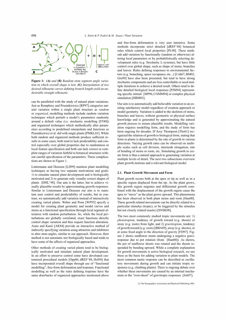
Figure 1: (A) and (B) Random stem segment angle varia-tion in which overall shape is lost. (C) Interpolation of twodesired silhouette curves defining branch length yield an un-desirable straight silhouette.

can be paralleled with the study of natural plant variations.Just as Remphrey and Prusinkiewicz [RP97] categorize nat-ural variation within a single plant structure as randomor organized, modelling methods include random variationtechniques which perturb a model’s parameters randomlyaround a default value (i.e. stochastic modelling [FF80])and organized techniques which methodically alter param-eters according to predefined interpolants and functions asPrusinkiewicz et al. did with single plants [PMKL01]. Whileboth random and organized methods produce sufficient re-sults in some cases, both tend to lack predictability and con-trol especially over global properties due to randomness orlocal feature specification and both can lack correct or com-plete ranges of variation faithful to botanical structures with-out careful specification of the parameters. These complica-tions are shown in Figure 1.

Lintermann and Deussen [LD99] mention plant modellingtechniques as having two separate motivations and goals:1) to simulate natural plant development and is biologicallymotivated and 2) to generate only visually correct shapes ofplants [DHL∗98]. Our aim is the latter, but to achieve vi-sually plausible results by approximating growth responses.Similar to Lintermann and Deussen our aim is to main-tain user control and predictability of results, but in con-trast, we automatically add variation instead of interactivelycreating varied plants. Weber and Penn [WP95] specify amodel for creating plant geometry and model curves andstems as a functional specification through local segment al-teration with random perturbation. So, while the local per-turbations are globally correlated, exact functions directlycontrol shape variation and thus require function alteration.Aono and Kunii [AK84] provide an interactive method ofindirectly specifying variation using attractors and inhibitorsto alter stem angles, similar to our approach. However, theirmethod is not automatic nor biologically based and tends tohave some of the affects of organized approaches.

Other methods of creating varied plants tend to be biolog-ically motivated and simulate natural plant development.In an effort to preserve control some have developed cus-tomized procedural models [Opp86, dREF∗88, Hol94] thathave incorporated overall shape through use of “functionalmodelling”, free-form deformation and tropisms. Functionalmodelling as well as the rules defining tropisms have thesame drawbacks of organized approaches mentioned above

and free-form deformation is very user intensive. Somemethods incorporate strict detailed [dREF∗88] botanicalrules which control local properties [PL90]. These meth-ods add variation by functionally (random or otherwise) al-tering local parameters or by probabilistically selecting de-velopment rules (e.g. Stochastic L-systems), but have littlecontrol over global shape, such as shape of stems, branchesand leaves. Rules defining responses to environmental fac-tors (e.g. branching, space occupancy etc...) [Coh67, BM02,Gre89] have also been presented, but tend to have strongstochastic components and are less controllable or need mul-tiple iterations to achieve a desired result. Others tend to de-fine detailed biological local responses [PJM94] represent-ing specific stimuli [MP96,COMM94] or complex physicalsimulation [HBM03].

Our aim is to automatically add believable variation to an ex-isting satisfactory model regardless of creation approach ormodel geometry. Variation is added to the skeleton of stems,branches and leaves, without geometric or physical surfaceknowledge and is generated by approximating the naturalgrowth process to ensure plausible results. Modelling vari-ation requires modelling form, and the study of form hasbeen ongoing for decades. D’Arcy Thompson [Tho61] rec-ognized the relation of growth to biological form, stating thatform in plants is determined by the rate of growth in variousdirections. Varying growth rates can be observed on multi-ple scales such as cell division, internode elongation, rateof bending of stems or roots, etc. Simulating growth to cre-ate form is thus a natural approach to generating variation atmultiple levels of detail. The next two subsections overviewplant growth motions and a relevant biological model.

2.1. Plant Growth Movement and Form

Plant growth occurs both at the apex or tip as well as in aspecific region displaced from the tip. As the plant grows,this growth region migrates and differential growth com-bined with the displacement of the growth region cause theapex to “move” as the plant grows upward. This phenomenahas been observed in both plant stems and roots [Han00].These growth related movements can be directly related to aparticular stimulus (tropic), or be triggered by the stimulusbut not closely related (nastic) [SNSK08].

The two most commonly studied tropic movements are: 1)phototropism, tendency of growth toward (e.g. shoots) oraway (e.g. roots) from light, and 2) gravitropism, tendencyof growth toward (e.g. roots) [BBA89], away (e.g. shoots), orat some fixed angle to the direction of gravity [FD97]. Fig-ure 2 shows sunflower stems undergoing a negative gravi-response due to pot rotation (from [Han00]). As shown,the pot of sunflower shoots was rotated and the shoots re-sponded by bending upward. While a complete explanationfor growth movements is active biological research, we usethese as the basis for adding variation to plant models. Themost common nastic response can be described as oscilla-tory movements during growth and can initiate tropic re-sponses (e.g. climbing plants). There is ongoing debate overwhether these movements are caused by an internal mecha-nism or the “over-shoot” of gravitropic responses [Joh97].

c© The Eurographics Association and Blackwell Publishing 2005.

498


Animation frames from Roger Hangarter [Han00] with permission.

Figure 2: Within one hour of pot displacement the sunflower shoots responded negatively (away) to gravity. Frames at 0, 40,60, 90 and 120 min. after displacement.

2.2. Biological Models of Movement and Growth

The majority of gravitropic response research has beenwith roots because of their quick response, relatively sim-ple structure, and suitability for laboratory experimentation[BPB94]. Observations and models in this area are summa-rized here. Roots have a region of growth displaced fromthe root cap or tip (see Figure 3(c)). Darwin [Dar80] con-cluded that the root cap is necessary for gravitropic sensingand determination of the root’s gravitropic response. Barlowet. al. [BBA89] concluded that growth rates (RELELs - rela-tive elemental rates of elongation) may differ around the rootwithin the growth region. They used RELELs to character-ize the growth pattern over the organ, creating differentialgrowth and curvature.

Edited from [BBA89]

(a) (b) (c)

Figure 3: (a) Root tip bending. (Mu,Ml) = (2.0,1.0), (μu =μl) = 3.0, σu = σl = 1, tip angles: t = (0.126,0.380,0.633),θ =(18.1,54.5,90.8) (b) μ , σ alteration. (Mu,Ml) = (3.0,1.0),(μu,μl) = (3.0,5.0), (σu,σl) = (0.7,1.0) (c) Illustration of rootand substance transport.

Barlow et al. [BBA89, ZBB97] model a plant root as aconstant-diameter d cylinder. They simulate a 2D longitudi-nal slice of the root, constraining bending within the plane.A RELEL is assumed for each point s at time t on the up-per Lu and lower Ll flanks of the slice and is associatedwith an angle of the tip to the vertical (displacement) θ atsome earlier time t ′. The time-lapse indicates lag betweenthe sensed displacement and the resulting response. Differ-ential growth results from asymmetric RELELs. They useda Gaussian distribution of RELELs = Mexp(−(x−μ)2/2σ2

where x is the distance from s to the tip, μ is the value of xat the maximum M RELEL, and σ is the distance from μwhere RELEL = 0.607M. Differences in parameters causegrowth rate differences around the root at a given time.

The tip angle θ at any time is determined by the lengths ofLu and Ll . Varying M while keeping σ and μ the same for Lu

and Ll alters the growth rate and flank length proportional toM with proportionality constant α as follows:

θ =Lu −Ll

d=

α(Mu −Ml)d

(1)

This achieves bending over time (see Figure 3a). Varyingσ independently on Lu and Ll results in curves of differentradii, and altering μ over time can form kinked shapes simi-lar to corn roots [BBA89, p.79](see Figure 3b).

Barlow et al. [BBA89, p.79] suggest achieving more elabo-rate curves through complex rearrangements of growth rates(e.g. θ a function of other parameters like μ or asymmetricRELEL distributions) or interactions of different tropisms.Barlow et al. [BPB94] note two more results of interest toour approach. First, the rate of bending is constant indepen-dent of θ . Second, the relation of the lag (between sensorand response) to the response, can cause bending to over-shoot the target re-initiating an gravitropic response on theother side to simulate the commencement of nutation. Therelation of the tip angle to overall shape and the observationof the relation between lag and response forms the basis ofthe structural approach described in Section 4.

3. Surface-based Variation

Our first approach to modelling variations simulates alter-ations in surface growth rate of a root according to theuneven distribution of a plant hormone called auxin. Theauxin concentration inhibits growth leading to bending.The impact of differences in growth rate on resulting rootshape is comparable with how the distribution of Barlow’sRELELs [BBA89] affects the resulting tip angle of a root.This biological simulation is used to verify the results of ourskeletal based method presented in Section 4.

The assumptions we used to construct our model were takenfrom [MTR∗04], and are briefly outlined below. Auxin istransported through the root’s center toward the tip at someconstant rate. The auxin is then distributed at the tip by agravitropic mechanism, as a function of orientation of thetip with respect to the gravity vector (angle θ see Figure 3a).A larger fraction of the available auxin is redirected to theside of the root tip that is oriented toward gravity. When thedirection of the tip and gravity match, auxin is equally dis-tributed. Once the auxin is distributed at the tip, it is trans-ported by a polar transport mechanism along the surface ofthe root back toward the plant, as illustrated in Figure 3c.Auxin modulates growth rates within the growth zone by in-hibition. Uneven auxin concentrations cause uneven (differ-ential) growth and consequent bending, a behavior consis-tent with Barlow et al. models [BBA89, ZBB97]. Bendingcontinues until the tip is realigned with gravity and an evendistribution of auxin is restored.

Based on the above assumptions, we constructed the follow-


499


root tipsegment

segment

growth zone

less auxin

more auxin

gravity

a)

b)

c) d)

Figure 4: (a-c) Simulation model of a gravitropic response in a developing root. (d) Various root shapes produced by the model.

ing two-dimensional simulation. We first discretize the rootinto multiple segments and a single root tip segment, as il-lustrated in Figure 4a. Each segment is associated with twotypes of information, the level of auxin at its top and bottomsides, and the segment’s shape. The segments are initiallyrectangular, although they deform throughout the simula-tion. The core of the simulation consists of the main loop,where the development of the root is incrementally simu-lated in time steps of Δt.

Each iteration through the main loop consists of three steps.First, we calculate the concentrations changes of auxin ineach segment in time Δt. This amounts to simulating polartransport oriented in the direction away from the root tip andaccounting for addition of new auxin at the root tip fromthe root center and re-distributing it by the gravity sensingmechanism.

In the second step, after the new values of auxin in each seg-ment are calculated, we simulate the growth of each seg-ment. The shape of each segment is changed by elongatingtheir top and bottom sides according to growth rate, similarto RELELs [BBA89]. The growth rate of a particular side ofa segment is a function of two variables: the distance fromthe root tip, and the concentration of auxin at the side of thesegment. The distance from the root tip determines the lo-cation of the growth zone [BBA89]. The root grows fasternear the center of the growth zone and tapers off away fromthe center. This preliminary rate is then modified accordingto the level of auxin associated with the side of the segment.The resulting growth rate is then applied to calculate the newlengths of the sides of each segment and update the segmentshape, resulting in rhomboidal-shaped segments (Figure 4b).To prevent segments from becoming too large, they are dy-namically subdivided upon reaching a threshold size.

In the final step of the simulation loop, after the individ-ual segment shapes have been computed, we assemble theresulting root shape as illustrated in Figure 4c. This is ac-complished by first fixing the last segment of the root tosome predefined location. The next adjacent segment is thentranslated and rotated so that its left side matches the last

segment’s right side. This process is repeated iteratively un-til the shape of the whole root is reconstructed. The rootbending is thus an emergent phenomenon in our simulations.Various root shapes obtained using our 2D simulation areshown in Figure 4d. These results were generated by vary-ing some of the simulation parameters, such as the size andlocation of the growth zone, the auxin transport rate, the in-hibition effect of auxin on growth, etc.

We also extended our gravitropic simulation of roots to threedimensions. We assume that the initial shape of the youngroot is cone-like, which we discretize into cylindrical seg-ments of equal heights. Each such segment’s surface is thendiscretized into a polygonal mesh. As the auxin is trans-ported through the segments’ surfaces, the mesh polygonsundergo growth. The result of uneven auxin distributions isnon-uniform growth, which manifests itself by transform-ing the initial cylinder-like segments into more wedge-likeshapes. By iteratively assembling the segments, similar tothe process described for the 2D model, the 3D shape of theroot can be reconstructed.

4. Skeletal-based Variation

We model plant variations through changes in the struc-ture or skeleton by abstracting the surface growth responsesshown in Section 3, and relating them to the plant skeletonand changes in tip angle similar to Barlow’s work (see Sec-tion 2.2). Starting from a base model skeletal representation,variations are added by simulating growth responses to influ-ences or stimuli (see Section 2). The skeleton is subdividedinto growth steps and at each step we monitor and respondto the difference between the desired (base model) and cur-rent growth directions. This mechanism is modelled using acontrol system.

We use a base model’s skeleton to define the desired direc-tion or natural course of growth. Then by subjecting thisskeleton to the same stimuli as real plants and compensat-ing for the surface offset from the skeleton, we apply adjust-ments directly to the skeletal representation. Once the mod-ified skeleton is obtained, the surface is recreated and a new


500


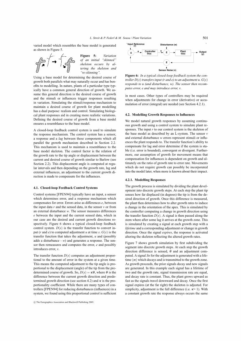
varied model which resembles the base model is generatedas shown in Figure 5.

Figure 5: Variationof an initial “skinned”skeleton occurs by al-tering the skeleton and“re-skinning”.

Using a base model for determining the desired course ofgrowth both parallels what may naturally occur and has ben-efits to modelling. In nature, plants of a particular type typ-ically have a common general direction of growth. We as-sume this general direction is the desired course of growthand the stimuli or influences trigger responses resultingin variation. Simulating the stimuli/response mechanism tomaintain a desired course of growth for plant modellinghas a dual purpose: realism and control. Simulating biologi-cal plant responses aid in creating more realistic variations.Defining the desired course of growth from a base modelensures a resemblance to the base model.

A closed-loop feedback control system is used to simulatethe response mechanism. The control system has a sensor,a response and a lag between these components which allparallel the growth mechanism described in Section 2.2.This mechanism is used to maintain a resemblance to thebase model skeleton. The control factor is the relation ofthe growth rate to the tip angle or displacement between thecurrent and desired course of growth similar to Barlow (seeSection 2.2). This displacement angle is computed at regu-lar intervals and then depending on the growth rate, lag andexternal influences, an adjustment to the current growth di-rection is made to compensate for the influences.

4.1. Closed-loop Feedback Control Systems

Control systems [FPEN94] typically have an input, a sensorwhich determines error, and a response mechanism whichcompensates for error. Errors arise as differences e, betweenthe input data r and the sensed data, in the sensor v or froman external disturbance w. The sensor measures differencese between the input and the current sensed data, which inour case are the desired and current growth directions re-spectively. Figure 6 shows a typical closed-loop feedbackcontrol system. D(s) is the transfer function to convert in-put (r and e) to computed adjustment u at time s. G(s) is thetransfer function that takes the adjustment, u and (possiblyadds a disturbance - w) and generates a response. The sen-sor then remeasures and computes the error, e and possiblyintroduces error, v.

The transfer function D(s) computes an adjustment propor-tional to the amount of error in the system at a given time.This means the computed adjustment to the tip angle is pro-portional to the displacement (angle) of the tip from the pre-determined course of growth. So, D(s) = κθ , where θ is thedifference between the current growth direction and prede-termined growth direction (see section 4.2) and κ is the pro-portionality coefficient. While there are many types of con-trollers [FPEN94] for reducing disturbances (influences) in asystem, we found using this proportional control is sufficient

ControllerD(s)

Output(y)G(s)

Plant

Disturbance (w)

Sensor Noise (v)

E E

E

e u

Input(r)Reference

Figure 6: In a typical closed-loop feedback system the con-troller D(s) transfers input (r and e) to an adjustment u. G(s)responds to u (and disturbance, w). The sensor then recom-putes error, e and may introduce error, v.

in most cases. Other types of controllers may be requiredwhen adjustments for change in error (derivative) or accu-mulation of error (integral) are needed (see Section 4.2.1).

4.2. Modelling Growth Responses to Influences

We model natural growth responses by assuming continu-ous growth and using a control system to simulate plant re-sponses. The input r to our control system is the skeleton ofthe base model as described by an L-system. The sensor vand external disturbance w errors represent stimuli or influ-ences the plant responds to. The transfer function’s ability tocompensate for lag and error determine if the system is sta-ble (i.e. error is bounded), convergent or divergent. Further-more, our assumption of growth for movement means thatcompensation for influences is dependent on growth and ul-timately on the ratio of growth rate to error rate. Movementswhich do not require growth can possibly be incorporatedinto the model later, when more is known about their impact.

4.2.1. Modelling Responses

The growth process is simulated by dividing the plant devel-opment into discrete growth steps. At each step the plant tipsenses how far displaced (in degrees) the tip is from the de-sired direction of growth. Once this difference is measured,the plant then determines how to alter growth rates to inducea change in the orientation of the apex. This is simulated bythe controller computing a change in growth direction usingthe transfer function D(s). A signal is then passed along thestem where after some lag it arrives at the growth zone. Thisis simulated by creating a signal at each growth step with alifetime and a corresponding adjustment or change in growthdirection. Once the signal expires, the response is activatedaltering the skeleton reflecting the altered growth rates.

Figure 7 shows growth simulation by first subdividing thesegment into discrete growth steps. At each step the growthdirection difference is sensed, θ and an adjustment com-puted. A signal Sn for the adjustment is generated with a life-time (m) which decays and is transmitted to the growth zone.As growth proceeds, the prior signals decay and new signalsare generated. In this example each signal has a lifetime oftwo and the growth rate, signal transmission rate are equal,and decay rate is constant. Thus, the plant grows upward asfast as the signals travel downward and decay. Once the firstsignal expires (at the far right) the skeleton is adjusted. Forsimplicity, adjustment is the full difference (i.e. κ= 1). Witha constant growth rate the response always occurs the same


501


Figure 7: At each step the growth direction difference, θ issensed and an adjustment computed. A signal Sn carries theadjustment which is activated when the signal “expires”.

distance from tip. By altering the growth rate, transmissionrate, lifetime (i.e how long a signal lasts with constant de-cay rate), or decay rate of various signals, the growth regionmay migrate causing signals to convolve, requiring integralor derivative control (see Section 4.1). In the examples re-ported in this paper, growth occurs in the growth zone (nearthe tip) only, however in plants growth also occurs as elonga-tion of stems. This may be simulated by similarly elongatingeach subdivided growth step and adjusting the signal decayappropriately.

4.2.2. Modelling Stimuli or Influences

There are two types of possible influences that causevariation: imperfect sensing and external or environmen-tal stimuli. The plant senses how far (angle) the apex isfrom the ideal predetermined direction or path of growthby sensing both the current growth direction Hcurr andthe desired or target growth direction Htar. In realitythere are numerous factors (e.g. hydration, growth rateetc.) that may cause imprecision in this measure. Due to

imperfect sensing, Hcurr may not accuratelyrepresent the current growth direction. In ourmodel the sensor error is approximated by ran-dom radial Gaussian distribution about Hcurr

as shown at left, creating the sensed growth di-rection Hsense. The difference in growth direc-tions is then determined by computing the an-

gular difference between two normalized vectors, Hsense andHtar as: acos(Hsense ·Htar). The controller uses this differ-ence to compute an adjustment (see Section 4.1).

While adjustment computation is exact using the definedtransfer function and the sensed difference, the plant mayreact without knowledge of external stimuli. The externalstimuli represent environmental factors that may affect thegrowth direction aside from those which define the pre-determined course of growth. Since these factors (e.g. wind,growth proximity etc.) are so numerous we model them intwo ways: randomly and functionally. The random modelrepresents the statistical averaging of numerous seeminglyrandom factors resulting in a random influence with a Gaus-sian or uniform distribution. Alternatively, to explore howa specific, possibly dominant, stimulus affects the growthdirection, a function can be specified which represents thisstimulus or overall target growth direction. Figure 8 showstwo examples of user specified target (left bottom) and dis-turbance functions (left top). These functions are appliedwith the target function in one orthogonal plane (middle) todefine overall shape and the disturbance in a second orthog-onal plane to show local variation (right). A more integrated

Disturb.

Target

Disturb.

Target

Figure 8: Two examples of user specified functions (left)applied orthogonally (right).

example of the use of target function specification is shownin Figure 13 and is detailed in Section 5.

The difference between imperfect sensing and external stim-uli is, the former is directly compensated for by the con-troller, while external stimuli are only compensated at thenext stage of sensing and correction (see Figure 6). Conse-quently, imperfect sensing impacts variation less.

4.3. The Process and Form

In addition to growth and error rate affecting form, the lagbetween the determination and activation of a response, asnoted by Barlow et. al [BPB94] also affects form. In realplants the relation between lag and growth rate is not clear.In our model it is a ratio between the lag and the ability to ad-just (i.e. size of adjustment κ see Section 4.1) that impactsform the most. This ratio represents the plant response tostimuli and will be called the compensation ratio. The mag-nitude of the lag reflects the rate of response. The magnitudeof the adjustment, determined by transfer function D(s), re-flects the number of adjustments required to compensate foran influence. No adjustment can be made without a responsefirst signaling an adjustment, coupling these parameters intothe compensation ratio. To provide an intuition and relationto the feedback control mechanism with a single initial dis-turbance, error E(n) (i.e. θ ) at growth stage n, obeys the re-currence relation: E(n) = E(n−1)−κE(n−1− lag), whereD(s) = κθ . The compensation ratio, (κ ∗ lag)−1 ≈ 0.7 hasbeen experimentally determined to represent a stable systemand is discussed below.

Consider a single initial influence on a plant, whose desiredcourse of growth is straight upward (either toward a pointlight or away from gravity). The single influence simulatesa change relative to gravity direction by displacing the plant90◦ shortly after growth is commenced, similar to the sun-

Figure 9: Varying lag and adjustment ability. At 20% ofshown growth a 90◦ rotation occurred. Compensation ratio= 0.72, lag decreasing left to right. Compare with Figure 2.


502


flower animation in Figure 2. Figure 9 shows our model ofa plant reacting to being turned 90◦ at 20% of total showngrowth. Varying amounts of lag and adjustment ability areused, however, all compensation ratios are fixed at 0.72. Asthe lag magnitude decreases from left to right, the plant ad-justs to the stimuli more quickly. Note the small amount ofoscillation before convergence to the pre-determined coursein the two rightmost plants due to the significant “over-shoot” of the target.

The two parameters for controlling variation given a baseskeleton, are the lag and the adjustment ability κ , which to-gether form the compensation ratio. As shown in Figure 9maintaining a constant compensation ratio and altering lagmagnitude (i.e. altering κ proportionally to lag) introducesvariation at different levels of detail. The plant on the farright has variation of a much higher frequency than the planton the far left. The overall plant shape is controlled usingthe base skeleton model and as shown all plants achievea general upward course of growth despite being turned90◦. Altering the compensation ratio (i.e. changing lag dis-proportionally to κ) can alter the change in variation overgrowth as shown below. A compensation ratio from 0.5 to1.2 effectively alters variation. The sensitivity of variation tolag magnitude depends on the number of subdivided growthsteps used. All examples in this paper had lag ∈ [4%−30%]of the number of subdivided growth steps.

As the compensation ratio is altered, the plant either com-pensates equally for the stimulus, under-compensates orovercompensates. If the plant equally compensates for thestimulus given the lag, then regular oscillation may occur.The lag is long enough, relative to the adjustment and stim-uli magnitude, such that the adjustments regularly overshootthe target by a constant amount causing oscillation. How-ever, if the plant under-compensates or overcompensates ei-ther a divergent or convergent form results, meaning that theplant either overshot the target by a increasing or decreasingamount respectively as shown in Figure 10. The plants wererotated 20◦ at the start of growth. The group of stalks onthe left have shorter lag than those on the right. Within eachgroup the compensation ratio is increased from left to rightto exhibit under-compensation, equal and overcompensationof the stimuli, respectively.

Figure 10: Two groups of differing lag and adjustment abil-ities. Left: smaller lag Right: larger lag. In each group theadjustment ability is under-compensated (left), equal (cen-ter) and over-compensated (right).

4.4. Implementation and L-system Details

The skeleton is sequentially varied proceeding from the rootto the tip by adding variation to each subdivided skeletalsegment (see Section 4.2.1). Assuming the existence of amethod STRAIGHSKEL() for creating a straight skeletal seg-ment of length l, we devised an algorithm to create a variedskeletal segment of the same length as shown below.CREATEVARIEDSKEL(l)1 currlen ← 02 while currlen �= l3 do Get Hsense and Htar // Sensor measure with error4 e ← GETERROR(Hsense,Htar)5 t ← GETSIGNALLIFETIME()6 U ← COMPADJ(e) // Controller D(s) & influence7 ADJUST(t,U ) // Signal a response8 STRAIGHTSKEL(δ l) // Continuous growth9 currlen ← currlen+δ l

ADJUST(t,U )1 if signal t has expired2 then Plant G(s) activates adjust. of segment by U3 else δ t ← ELAPSEDAGE() // Decay & pass signal4 ADJUST(t −δ t,U )In our algorithm, small segments δ l are altered in orienta-tion to create variation over length l. Note that segment ad-dition or growth is continuous and an adjustment is madeeach time a subsegment δ l is added. However, the growthrate can be varied by altering δ l over time. In relation to thecontrol system in Figure 6, at each growth step the sensordetects the current and target growth directions (line 3) andmeasures the error (line 4). The controller then computes anadjustment in orientation (line 6) and creates a response sig-nal with lifetime t (lines 5 and 7). This process is repeateduntil the length l is achieved.

While our algorithm is general enough to introduce variationto any skeletal model defining Htar, we have chosen to usean L-system as the base model’s skeleton and consequentlyimplement the algorithm as an L-system. The details neededto convert most L-system plant descriptions to one whichintroduces variation is given in the appendix.

5. Results

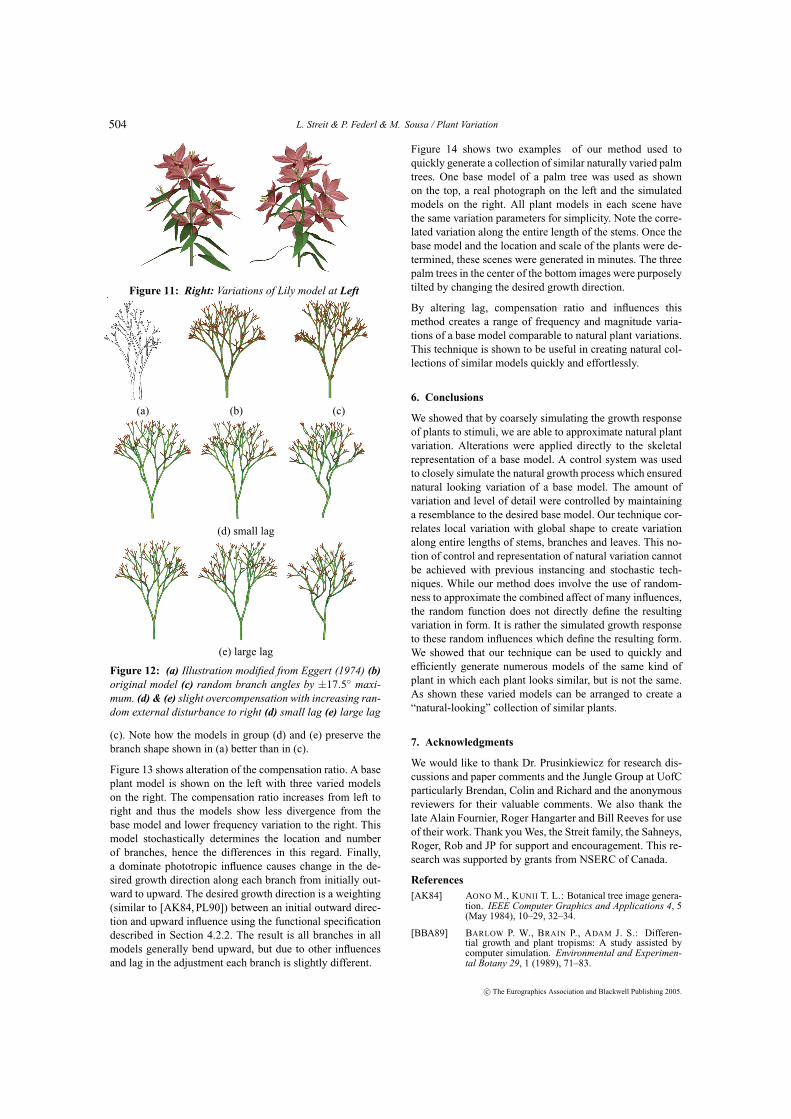
Once the L-system is modified, the varied skeleton is gen-erated in seconds on a 800MHz PIII with a GeForce FXgraphics card. The development of the variation is, of course,directly dependent on the number of subsegments used. Fig-ure 11 shows the base Lily model (left) and a varied model(right). This model has a compensation ratio of ≈ 0.7 andlarge lag shown by the stem, branch and leaf curvature.

Figure 12 shows a model of Horneophyton with constantcompensation ratio and differing amounts of lag and influ-ences. An illustration and base model (L-system) are shownin (a) and (b). A constant compensation ratio is maintained,but altering lag results in variation of different frequencies(compare group d with e) and altering the magnitude ofthe influence or stimuli alters the magnitude of the varia-tion (compare within group d or e). A model with stochas-tic branch angle variation by ±17.5◦ degrees is shown in


503


Figure 11: Right: Variations of Lily model at Left

(a) (b) (c)

(d) small lag

(e) large lag

Figure 12: (a) Illustration modified from Eggert (1974) (b)original model (c) random branch angles by ±17.5◦ maxi-mum. (d) & (e) slight overcompensation with increasing ran-dom external disturbance to right (d) small lag (e) large lag

(c). Note how the models in group (d) and (e) preserve thebranch shape shown in (a) better than in (c).

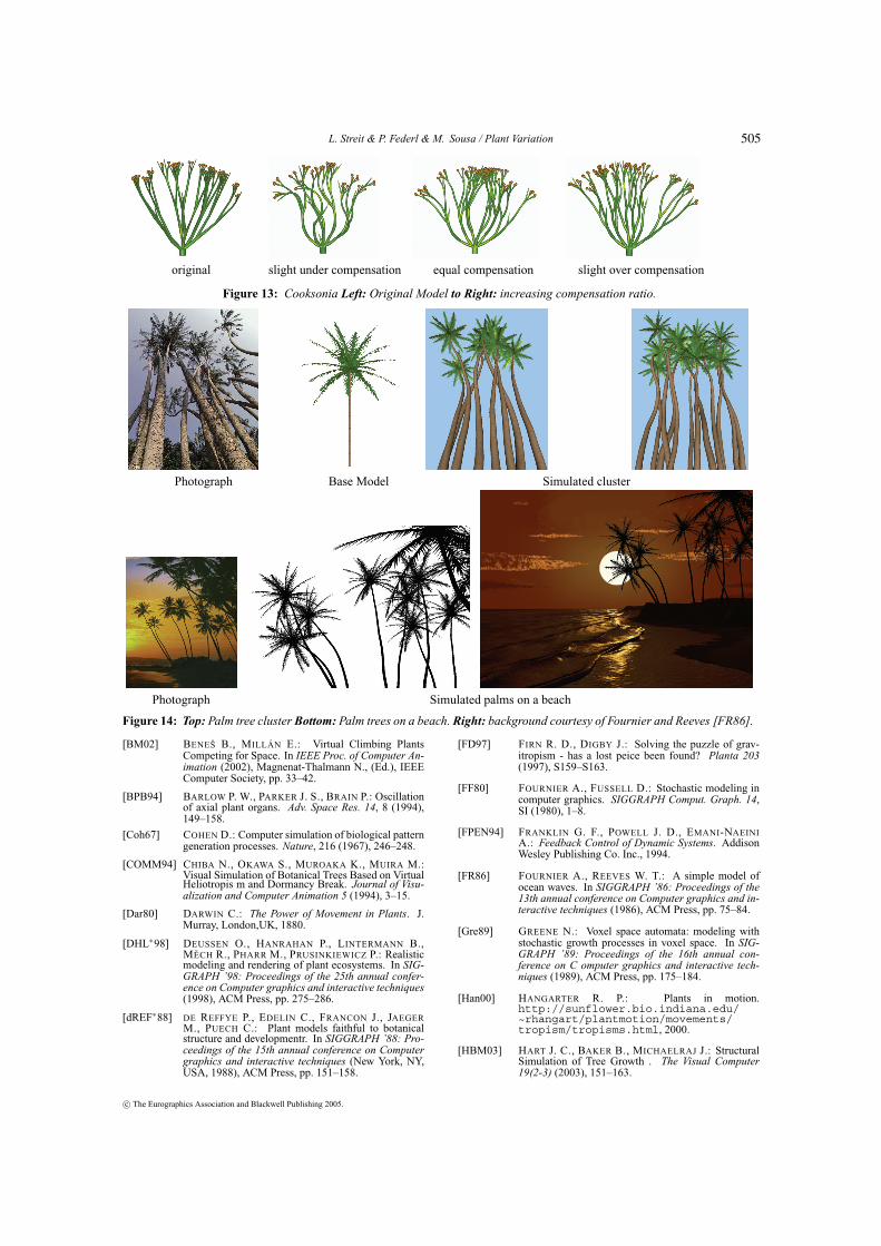
Figure 13 shows alteration of the compensation ratio. A baseplant model is shown on the left with three varied modelson the right. The compensation ratio increases from left toright and thus the models show less divergence from thebase model and lower frequency variation to the right. Thismodel stochastically determines the location and numberof branches, hence the differences in this regard. Finally,a dominate phototropic influence causes change in the de-sired growth direction along each branch from initially out-ward to upward. The desired growth direction is a weighting(similar to [AK84, PL90]) between an initial outward direc-tion and upward influence using the functional specificationdescribed in Section 4.2.2. The result is all branches in allmodels generally bend upward, but due to other influencesand lag in the adjustment each branch is slightly different.

Figure 14 shows two examples of our method used toquickly generate a collection of similar naturally varied palmtrees. One base model of a palm tree was used as shownon the top, a real photograph on the left and the simulatedmodels on the right. All plant models in each scene havethe same variation parameters for simplicity. Note the corre-lated variation along the entire length of the stems. Once thebase model and the location and scale of the plants were de-termined, these scenes were generated in minutes. The threepalm trees in the center of the bottom images were purposelytilted by changing the desired growth direction.

By altering lag, compensation ratio and influences thismethod creates a range of frequency and magnitude varia-tions of a base model comparable to natural plant variations.This technique is shown to be useful in creating natural col-lections of similar models quickly and effortlessly.

6. Conclusions

We showed that by coarsely simulating the growth responseof plants to stimuli, we are able to approximate natural plantvariation. Alterations were applied directly to the skeletalrepresentation of a base model. A control system was usedto closely simulate the natural growth process which ensurednatural looking variation of a base model. The amount ofvariation and level of detail were controlled by maintaininga resemblance to the desired base model. Our technique cor-relates local variation with global shape to create variationalong entire lengths of stems, branches and leaves. This no-tion of control and representation of natural variation cannotbe achieved with previous instancing and stochastic tech-niques. While our method does involve the use of random-ness to approximate the combined affect of many influences,the random function does not directly define the resultingvariation in form. It is rather the simulated growth responseto these random influences which define the resulting form.We showed that our technique can be used to quickly andefficiently generate numerous models of the same kind ofplant in which each plant looks similar, but is not the same.As shown these varied models can be arranged to create a“natural-looking” collection of similar plants.

7. Acknowledgments

We would like to thank Dr. Prusinkiewicz for research dis-cussions and paper comments and the Jungle Group at UofCparticularly Brendan, Colin and Richard and the anonymousreviewers for their valuable comments. We also thank thelate Alain Fournier, Roger Hangarter and Bill Reeves for useof their work. Thank you Wes, the Streit family, the Sahneys,Roger, Rob and JP for support and encouragement. This re-search was supported by grants from NSERC of Canada.

References[AK84] AONO M., KUNII T. L.: Botanical tree image genera-

tion. IEEE Computer Graphics and Applications 4, 5(May 1984), 10–29, 32–34.

[BBA89] BARLOW P. W., BRAIN P., ADAM J. S.: Differen-tial growth and plant tropisms: A study assisted bycomputer simulation. Environmental and Experimen-tal Botany 29, 1 (1989), 71–83.


504


original slight under compensation equal compensation slight over compensation

Figure 13: Cooksonia Left: Original Model to Right: increasing compensation ratio.

Photograph Base Model Simulated cluster

Photograph Simulated palms on a beach

Figure 14: Top: Palm tree cluster Bottom: Palm trees on a beach. Right: background courtesy of Fournier and Reeves [FR86].

[BM02] BENEŠ B., MILLÁN E.: Virtual Climbing PlantsCompeting for Space. In IEEE Proc. of Computer An-imation (2002), Magnenat-Thalmann N., (Ed.), IEEEComputer Society, pp. 33–42.

[BPB94] BARLOW P. W., PARKER J. S., BRAIN P.: Oscillationof axial plant organs. Adv. Space Res. 14, 8 (1994),149–158.

[Coh67] COHEN D.: Computer simulation of biological patterngeneration processes. Nature, 216 (1967), 246–248.

[COMM94] CHIBA N., OKAWA S., MUROAKA K., MUIRA M.:Visual Simulation of Botanical Trees Based on VirtualHeliotropis m and Dormancy Break. Journal of Visu-alization and Computer Animation 5 (1994), 3–15.

[Dar80] DARWIN C.: The Power of Movement in Plants. J.Murray, London,UK, 1880.

[DHL∗98] DEUSSEN O., HANRAHAN P., LINTERMANN B.,MECH R., PHARR M., PRUSINKIEWICZ P.: Realisticmodeling and rendering of plant ecosystems. In SIG-GRAPH ’98: Proceedings of the 25th annual confer-ence on Computer graphics and interactive techniques(1998), ACM Press, pp. 275–286.

[dREF∗88] DE REFFYE P., EDELIN C., FRANCON J., JAEGERM., PUECH C.: Plant models faithful to botanicalstructure and developmentr. In SIGGRAPH ’88: Pro-ceedings of the 15th annual conference on Computergraphics and interactive techniques (New York, NY,USA, 1988), ACM Press, pp. 151–158.

[FD97] FIRN R. D., DIGBY J.: Solving the puzzle of grav-itropism - has a lost peice been found? Planta 203(1997), S159–S163.

[FF80] FOURNIER A., FUSSELL D.: Stochastic modeling incomputer graphics. SIGGRAPH Comput. Graph. 14,SI (1980), 1–8.

[FPEN94] FRANKLIN G. F., POWELL J. D., EMANI-NAEINIA.: Feedback Control of Dynamic Systems. AddisonWesley Publishing Co. Inc., 1994.

[FR86] FOURNIER A., REEVES W. T.: A simple model ofocean waves. In SIGGRAPH ’86: Proceedings of the13th annual conference on Computer graphics and in-teractive techniques (1986), ACM Press, pp. 75–84.

[Gre89] GREENE N.: Voxel space automata: modeling withstochastic growth processes in voxel space. In SIG-GRAPH ’89: Proceedings of the 16th annual con-ference on C omputer graphics and interactive tech-niques (1989), ACM Press, pp. 175–184.

[Han00] HANGARTER R. P.: Plants in motion.http://sunflower.bio.indiana.edu/~rhangart/plantmotion/movements/tropism/tropisms.html, 2000.

[HBM03] HART J. C., BAKER B., MICHAELRAJ J.: StructuralSimulation of Tree Growth . The Visual Computer19(2-3) (2003), 151–163.


505


[Hol94] HOLTON M.: Strands, gravity, and botanical tree im-agery. Comput. Graph. Forum 13, 1 (1994), 57–67.

[Joh97] JOHNSSON A.: Circumnutations: results from recentexperiments on earth and in space. Planta 203 (1997),S147–S158.

[KL02] KARWOWSKI R., LANE B.: Lpfg user’s man-ual. http://algorithmicbotany.org/lstudio/LPFGman.pdf, 2002.

[LD99] LINTERMANN B., DEUSSEN O.: Interactive mod-eling of plants. IEEE Comput. Graph. Appl. 19, 1(1999), 56–65.

[MP96] MECH R., PRUSINKIEWICZ P.: Visual models ofplants interacting with their environment. In Pro-ceedings of the 23rd annual conference on Computergraphics and interactive techniques (1996), ACMPress, pp. 397–410.

[MTR∗04] MOLENDIJK A. J., TIETZ O., RUPERTI B., PA-PONOV I. A., PALME K.: Mechanisms of cell polarityestablishment and polar auxin transport. In Polarityin Plants, Lindsey K., (Ed.). Ed.Blackwell publishing,CRC Press, 2004, pp. 192–240.

[Opp86] OPPENHEIMER P. E.: Real time design and anima-tion of fractal plants and trees. In SIGGRAPH ’86:Proceedings of the 13th annual conference on Com-puter graphics and interactive techniques (New York,NY, USA, 1986), ACM Press, pp. 55–64.

[PJM94] PRUSINKIEWICZ P., JAMES M., MěCH R.:Synthetic topiary. In SIGGRAPH ’94: Proceedings ofthe 21st annual conference on Computer graphics andinteractive techniques (New York, NY, USA, 1994),ACM Press, pp. 351–358.

[PL90] PRUSINKIEWICZ P., LINDENMAYER A.: The Algo-rithmic Beauty of Plants. Springer-Verlag, 1990.

[PMKL01] PRUSINKIEWICZ P., MÜNDERMANN L., KAR-WOWSKI R., LANE B.: The use of positional informa-tion in the modeling of plants. In Proceedings of ACMSIGGRAPH 2001 (Aug. 2001), Computer GraphicsProceedings, Annual Conference Series, pp. 289–300.

[RP97] REMPHREY W. R., PRUSINKIEWICZ P.: Quantifica-tion and modelling of tree architecture. In Plant toEcosystems, Michalewicz M. T., (Ed.). CSIRO Aus-tralia, 1997, pp. 45–52.

[SNSK08] STRASBURGER E., NOLL F., SCHENCK H., KARS-TEU G.: A text-book of Botany. Macmillan and Co.Ltd., London, 1908.

[Tho61] THOMPSON D. W.: On Growth and Form. Cambridgeat the University Press, New York, 1961.

[WP95] WEBER J., PENN J.: Creation and rendering of realis-tic trees. In SIGGRAPH ’95: Proceedings of the 22ndannual conference on Computer graphics and inter-active techniques (New York, NY, USA, 1995), ACMPress, pp. 119–128.

[ZBB97] ZIESCHANG H. E., BRAIN P., BARLOW P.: Mod-elling of root growth and bending in two dimensions.Journal of Theoretical Biology 184 (1997), 237–246.

Appendix A: L-system Implementation Details

The base skeleton generally defines the desired course ofgrowth and is described by a base plant’s L-system. TheL-system is a set of rules which define the plants construc-tion [PL90]. Implementing our algorithm as part of an L-system requires a few details. The variation is added as theL-system is evaluated requiring two events at each eval-uation stage: update of relative transformation matrix, TMand temporary halting of evaluation of the L-system while

Original L-system Modified L-system

A() → A() →+ \ F(k) ^ + F(l) M() + \ CVS(k,TM) ^ + CVS(l,TM)

group 1:M() < CVS(k,TM)

state = 2; numbranches++;produce . . . Variation(k,0,TM) . . . }

group 2:Variation(k,nl,TM):{

Htar ∗TM . . .if (nl < k)

produce . . . Variation(k, nl++,TM);else

numbranches--;if (numbranches == 0)

state = 1; produce M();

Table 1: Transition from original L-system description tomodified L-system creating variation [KL02].

a straight line production becomes a series of small subseg-ments altering orientation and introducing variation as out-lined. As mentioned some branches grow at a particular an-gle to either gravity or the main stem. This desired growthdirection is simulated by either a globally or locally accu-mulated transformation matrix, TM . TM transforms the de-sired growth direction to either a global (relative to grav-ity) or a local (relative to the parent stem) direction. Halt-ing the L-system is required since variation and start loca-tion/orientation of one segment is dependent on the previous.Introducing variation sequentially in this manner ensuresvariation continuity along the length of a branch or stem andpreserves discontinuities of the original base model.

L-systems, are inherently non-sequential and thus threemechanisms were used to ensure sequential evaluation: Ta-ble L-systems, context sensitivity and a semaphore. Table L-systems associate a state with each rule or production and asevaluation occurs only those rules in the current global stateare considered. Altering the state allows us to halt the orig-inal L-system and add variation. A marker M() provides acontext to be satisfied to ensure evaluation of only one seg-ment of a single branch at a time and also to prevent eval-uation of child branches before their parents to which theyare attached. The marker is initially placed at the beginningof the main axiom and migrates down the L-system string asevaluation occurs and variation is added. When variation ofone segment is complete, the marker is replaced adding a sat-isfying context to the next segment. Since multiple branchescan develop at once, parallel evaluation of branches is per-mitted. However, using a global state to maintain sequencingof variation causes problems. Thus, a counting semaphorenumbranches prevents state changes until all branches havecompleted variation of their current segment.

Changing a base L-system to introduce variation is fairlygeneric (see Table 1). Given a set of turtle transformations(i.e +,\,^) and turtle translations (i.e. F(l)), from a de-composed L-system two productions with different statesare added: CVS which Creates a Varied Segment and Vari-ation. As shown, these productions change the state, updatethe semaphore and add the context M() as outlined above.


506

modelling plant variation through growth - algorithmic...

Documents