improving the performance of tilapia farming under climate ... · pdf fileimproving the...
TRANSCRIPT

Tilapia is one of the most popular aquaculture species and is farmed in more than 120 countries and territories. A bioeconomic model on tilapia pond culture has
been developed by the Food and Agriculture Organization of the United Nations (FAO) based on experiences in China, the largest tilapia farming country. The results of the model indicate that the technical and economic performance of tilapia farming can be significantly improved by optimal selection of stocking
timing, fingerling size, stocking density, growing period (or crop length), harvest timing and harvest size according to technical, economic and climate factors.
Bioeconomic modelling can facilitate knowledge-based innovations for increasing technical and economic benefits through more efficient use of resources. Its
potential has yet to be adequately appreciated or utilized. This paper represents an effort to improve the situation.
608
FAOFISHERIES ANDAQUACULTURE
TECHNICALPAPER
ISSN 2070-7010
Improving the performance of tilapia farming under climate variation Perspective from bioeconomic modelling
I8442EN/1/01.18
ISBN 978-92-5-130162-3
9 7 8 9 2 5 1 3 0 1 6 2 3
ISSN 2070-7010
Cover photographs (farmed tilapia value chain in China; courtesy of Junning Cai):
Large photo (middle): 700 g tilapia just harvested
Small photos (counter clockwise from top-left corner):Tilapia pondsTilapia broodstockNursing tilapia frySorting tilapia fingerlings for saleWeighing tilapia fingerlingsTilapia feedLoading tilapia feed in an automatic feeding machineHarvesting tilapia from a pondWeighing and loading harvested tilapia in a truck for transportationLive tilapia sold in a supermarketLive tilapia sold in a seafood marketSteamed tilapia served in a seafood restaurant

Improving the performance of tilapia farming under climate variationPerspective from bioeconomic modelling
by
Junning CaiAquaculture OfficerFAO Fisheries and Aquaculture DepartmentRome, Italy
PingSun Leung ProfessorUniversity of Hawai‘i at ManoaHonolulu, United States of America
Yongju LuoProfessorGuangxi Academy of Fishery SciencesNanning, China
Xinhua YuanProfessorFreshwater Fisheries Research CenterWuxi, China
and
Yongming YuanProfessorFreshwater Fisheries Research CenterWuxi, China
FOOD AND AGRICULTURE ORGANIZATION OF THE UNITED NATIONSRome, 2018
FAOFISHERIES ANDAQUACULTURE
TECHNICALPAPER
608
The designations employed and the presentation of material in this information product do not imply the expression of any opinion whatsoever on the part of the Food and Agriculture Organization of the United Nations (FAO) concerning the legal or development status of any country, territory, city or area or of its authorities, or concerning the delimitation of its frontiers or boundaries. The mention of specific companies or products of manufacturers, whether or not these have been patented, does not imply that these have been endorsed or recommended by FAO in preference to others of a similar nature that are not mentioned. The views expressed in this information product are those of the author(s) and do not necessarily reflect the views or policies of FAO. ISBN 978-92-5-130162-3 © FAO, 2018 FAO encourages the use, reproduction and dissemination of material in this information product. Except where otherwise indicated, material may be copied, downloaded and printed for private study, research and teaching purposes, or for use in non-commercial products or services, provided that appropriate acknowledgement of FAO as the source and copyright holder is given and that FAO’s endorsement of users’ views, products or services is not implied in any way. All requests for translation and adaptation rights, and for resale and other commercial use rights should be made via www.fao.org/contact-us/licence-request or addressed to [email protected]. FAO information products are available on the FAO website (www.fao.org/publications) and can be purchased through [email protected]. This publication has been printed using selected products and processes so as to ensure minimal environmental impact and to promote sustainable forest management.
iii
Preparation of this document
A bioeconomic model has been developed by the Food and Agriculture Organization of the United Nations (FAO) based on experiences in China to show how optimal arrangements of farming operations can improve the technical and economic performance of tilapia pond aquaculture. This paper presents the methodology and results of the model. The results reveal the mechanisms and extent by which aquaculture performance can be improved through optimal farming arrangements. The methodology provides technical guidance on bioeconomic modelling in tilapia pond culture and aquaculture in general. Junning Cai, PingSun Leung, Yongju Luo, Xinhua Yuan and Yongming Yuan are acknowledged for their contribution to the development of the model and preparation of this document. Qian Chen, Zhongqiang Liu, Xiangjun Miao, Yannan Tong, Deqiang Wang, Maoyuan Wang, Jun Yang, Wei Ye, Lei Zhao, Quanfu Zhong are acknowledged for facilitating surveys of tilapia farming in China. José Aguilar-Manjarrez, Uwe Barg, Malcolm Beveridge, Qian Chen, Marc Fantinet, Emmanuel Frimpong, Mohammad Hasan, Elisabetta Martone, Francisco Javier Martínez-Cordero, Felix Marttin, Carlos Pulgarin, Melba Reantaso, Susana Siar, Weiwei Wang and Zongli Zhang are acknowledged for their valuable comments and suggestions provided in seminars or through the formal review of the paper. Danielle Rizcallah, Maria Giannini and Marianne Guyonnet are acknowledged for their assistance in editing and formatting, and José Luis Castilla Civit is acknowledged for layout and graphic design.
iv
Abstract
Tilapia is the world’s most popular aquaculture species, farmed mostly in earthen ponds. Experience in China, the largest tilapia farming country, is used to develop and calibrate a bioeconomic model of intensive tilapia pond culture. The model is used to simulate the impacts of climate, technical and/or economic factors on farming performance and examines the performance of various farming arrangements under different conditions. The simulation results indicate that: (i) an increase in feed price, an increase in mortality, or a decrease in fish price significantly reduces profitability, whereas an increase in the cost of seed, labour, rent, electricity or water management has smaller impacts on profitability; (ii) considering the impact of water temperature on fish growth, the profitability of a production cycle starting at the optimum timing may be twice as high as one starting at the worst possible time; (iii) farming arrangements that maximize the profit of individual fish crops may not maximize overall profitability because of path dependency of farming performance; (iv) optimal farming arrangements that maximize overall profitability can significantly improve economic performance; (v) given no price discrepancy against small-size fish, harvesting at about 300 g in two-year-five-crop arrangements could increase overall enterprise profitability by up to 50 percent compared with harvesting at > 500 g in one-year-two-crop arrangements; and (vi) a two-tier farming system that separates nursing and outgrowing ponds could allow one-year-three-crop arrangements that enhance profitability by up to nearly 90 percent compared with the one-year-two-crop arrangements. With more refined information on fish growth under different farming conditions, the model could become a decision-making tool to help farmers design optimal farming arrangements.
Cai, J.N., Leung, P.S., Luo, Y.J., Yuan, X.H. & Yuan, Y.M. 2018.Improving the performance of tilapia farming under climate variation: perspective from bioeconomic modelling. FAO Fisheries and Aquaculture Technical Paper No. 608. Rome, FAO.

v
Contents
Preparation of this document iiiAbstract ivFigures viTables viiAbbreviations and acronyms viii
1. Introduction 1
2. A basic bioeconomic model on tilapia pond culture 5
2.1 Biological component of the basic model 52.2 Technical and economic parameters used in the basic model 92.3 Assessing the performance of tilapia pond culture in the basic model 10
3. An advanced bioeconomic model on pond tilapia culture 23
3.1 An advanced bioeconomic model that captures seasonal variation in the water temperature 23
3.2 Impacts of stocking timing on farming performance 293.3 Impacts of stocking density on farming performance 33
4. Optimizing crop arrangements for better performance 37
4.1 Profit maximization for individual crops ≠ overall profit maximization 38
4.2 Benchmark arrangement: 1 year 2 crops 38
4.3 Harvesting smaller size fish 47
4.4 Multi-tier farming systems 53
5. Discussion 61

vi
Figures
Figure 1: Original versus adjusted weekly weight gain 8Figure 2: Original versus adjusted feeding ration 8Figure 3: Weekly feed conversion ratio (FCR) 9Figure 4: Profit per crop for different growth periods 12Figure 5: Profit per week for different growing periods 14Figure 6: Marginal profit versus average profit 14Figure 7: Marginal revenue and marginal cost 15Figure 8: Marginal production versus average production 16Figure 9: Cost per unit of production, aka break-even price 17Figure 10: Breakdown of major cost items 18Figure 11: Cost structure 19Figure 12: Linear interpolation of feeding rations 24Figure 13: Linear interpolation of adjustment factors for feeding rations
under different water temperature 25Figure 14: Linear interpolation of the feed conversion ratios (FCRs) 26Figure 15: Correlation between weight gain minus feed use and fish biomass 27Figure 16: Fish growth path under different stocking densities (1 g fingerlings
and 28 °C water temperature) 28Figure 17: Calibrating the seasonal variation of water temperature in the
advanced model 30Figure 18: Average weekly water temperature and corresponding temperature
adjustment factors 31Figure 19: Profitability of individual crops under different stocking timings 31Figure 20: Growth patterns and farming performance of individual crops under
different stocking timings (1 g fingerlings, 1 200 fish/mu) 32Figure 21: Growth patterns and farming performance of individual crops under
different stocking density (1 g fingerlings) 34Figure 22: Impact of stocking timing and density on profitability 36Figure 23: Impact of stocking density on profitability under seasonal variations
in the water temperature 36Figure 24: Overall profitability under 1 year 2 crops (1 g fingerlings) 39Figure 25: Most versus least profitable arrangements under 1 year 2 crops
(1 g fingerlings) 41Figure 26: Growing period under 1 year 2 crops (1 g fingerlings) 42Figure 27: Stocking density and stocking timing under 1 year 2 crops 43Figure 28: Stocking density and water temperature under 1 year 2 crops 43Figure 29: Stocking density and harvest size under 1 year 2 crops 44Figure 30: Overall productivity and profitability under 1 year 2 crops 45Figure 31: Productivity and profitability by crop under 1 year 2 crops 46Figure 32: Profitability – 2 years 4 crops versus 1 year 2 crops 46Figure 33: Overall profitability of 1 year 2 crops under no price discrepancy
for small fish 48Figure 34: Profitability and productivity – 2 years 5 crops versus 1 year 2 crops 49Figure 35: Costs of fingerlings of different sizes 58Figure 36: Average production cost of large fingerlings 58Figure 37: Profitability and productivity – 1 year 3 crops versus 1 year 2 crops 59

vii
Tables
Table 1: GIFT tilapia growth pattern provided by the literature 6
Table 2: Tilapia growth pattern used to calibrate the basic model 7
Table 3: Technical and economic parameters used in the basic model 10
Table 4: Technical and economic performance of intensive tilapia pond culture in the basic model 13
Table 5: Impact of technical or economic factors on profitability and optimal harvest time 21
Table 6: Adjustment factors for feeding ration under different water temperatures 25
Table 7: Optimal farming arrangements and performance under different stocking density 34
Table 8: Profit maximizing arrangements under 1 year 2 crops (1 g fingerlings) 40
Table 9A: 2-year-5-crop arrangements under 1 g fingerlings and no price discrepancy between small and large fish 50
Table 9B: Productivity and profitability for the 2-year-5-crop arrangements in Table 9A 51
Table 10: Technical parameters used in the simulation of the production of large fingerlings 53
Table 11: Production of large-size fingerlings 55
Table 12A: 1-year-3-crop arrangements that maximize the overall profit for each of the 52 initial stocking timings 56
Table 12B: Productivity and profitability for the 1-year-3-crop arrangements in Table 12A
Table 13: Comparison of technical and economic performance of different crop arrangements 59
Table 14: Arrangements that maximize the profitability under 1 year 3 crops 59

viii
Abbreviations and acronyms
CNY Chinese YuanCP crude proteinFCR feed conversion ratioGIFT genetically improved farmed tilapiaWG weight gain

1
1. Introduction
Aquaculture is a complicated business, both technically and economically. The performance of an aquaculture operation is affected by a variety of environmental, technical and economic factors, such as climate, infrastructure, water quality, soil quality, seed quality, fish growth, feed quality, feed conversion ratio (FCR), disease, infrastructure, feed price, seed price, labour cost, other input prices, fish price and regulations. Farmers may not have much control over factors such as climate, infrastructure, market conditions and regulations, yet they can improve farming performance through good aquaculture practices and better business and operational planning. In a nutshell, business and operational planning in aquaculture is about selecting appropriate farming practices and arrangements to achieve business and operational goals (e.g. profit maximization). In this technical paper, a bioeconomic model is developed based on experiences in China to facilitate business and operational planning for improving the technical and economic performance in tilapia pond culture.
Tilapia is one of the most popular aquaculture species and is farmed in more than 120 countries and territories. However, global tilapia aquaculture production is highly imbalanced, with the top ten countries in 2015 accounting for over 90 percent of the 5.7 million tonnes of global production. China is the largest tilapia farming country, and in 2015 its share in the global production of tilapia was over 30 percent. There is a huge untapped potential in tilapia farming in other regions of the world, such as in sub-Saharan Africa where tilapia are native species and favoured by local consumers. Low productivity, however, is a key factor that affects the performance of tilapia farming in many countries. While it is common for a tilapia farmer in China to harvest 15 tonnes/ha per crop through intensive pond culture, the yield of pond tilapia culture in Africa is often less than 5 tonnes/ha per crop (FAO, 2017). Even tilapia farmers in China face constant pressure to improve productivity in order to offset the impacts of higher input costs, for example, land rental, feed and labour.
While advancement in technology, seed quality, feed quality and husbandry are key drivers for improving the performance of aquaculture, better business and operational planning is equally important. Planning an aquaculture operation involves arrangements of stocking timing, fingerling size, feeding regime, fertilizing scheme, water quality management, fish health management, growing period (or crop length),1 harvest timing, harvest size, among others. Fish farmers usually plan their operations based on common practices, experiences and/or expert advice. Farmers continually accumulate experiences in good farming practices and arrangements through trial and error, learning by practicing, and knowledge-sharing among peers. Through research and experiments, the research community generates information and knowledge to provide guidance on (optimal) arrangements of stocking density (Kazmierczak and Caffey, 1996; Liu and Chang, 1992); feeding regime (Esmaeili, 2005; Arnason, 1992); fertilization (Stickney et al., 1979); growing period or harvest timing or harvest size (Zuniga-Jara and Goycolea-Homann, 2014; Domínguez-May et al., 2011; Seginer and Ben-Asher, 2011; Yu and Leung, 2009; Yu, Leung and Bienfang, 2006; Yu and
1 Crop length is equal to the growing period plus time used for pond preparation after harvest. In the bioeconomic models here, the time for pond preparation is treated as an exogenous constant (i.e. two weeks); thus, selections of growing period and crop length are equivalent. The two terms are therefore used interchangeably in some places. Growing period is used when the time span between stocking and harvest needs to be specified, whereas crop length is used to calculate performance indicators such as profit per week or production per week.
Improving the performance of tilapia farming under climate variation: perspective from bioeconomic modelling2
Leung, 2005; Leung, Shang and Tian, 1994; Springborn et al., 1992; Arnason, 1992; Leung et al., 1989; Bjørndal 1988); and business management (Engle and Neira, 2005; Sanchez-Zazueta, Martinez-Cordero and Hernández, 2013), among others.
Bioeconomic models on tilapia farming in the literature are often built on an explicit, continuous fish growth function (Zuniga-Jara and Goycolea-Homann, 2014; Domínguez-May et al., 2011). Optimal farming arrangements in such models can be solved through mathematical derivations. However, the model setups and mathematical derivations are usually too complicated for farmers or extension personnel to decipher, which makes the results difficult to understand.
The bioeconomic model in this paper is a discrete, daily model calibrated from fish growth patterns under a certain feeding regime. The model set-up is in line with the financial analysis commonly used in business and investment planning. A large number of arrangements are simulated in the model, and the arrangements that give the best performance are identified by comparisons. This brute force method is less elegant than solving the optimal arrangements through mathematical derivations, and in some occasions possible arrangements are too many to be simulated comprehensively. But the method makes it easy to compare optimal arrangements with suboptimal alternatives so that the results can be better understood.
In the next section, a basic version of the bioeconomic model is presented. Water temperature, fingerling size and stocking density are fixed in the basic model to facilitate the examination of an optimal growing period that maximizes the profit in a single crop. The result indicates that when stocking 1 g of genetically improved farmed tilapia (GIFT) fingerlings at 1 200 fish/mu under constant water temperature at 28 °C,2 the optimal arrangement is to harvest 707 g fish after 21 weeks of the growing period.3 The model is used to illustrate how technical and economic factors affect farming performance and to demonstrate that arrangements that maximize productivity may not be profit maximizing.
The model is also used to examine the impacts of technical or economic factors (fish price, input prices and mortality) on profitability and optimal growing period. The results indicate that a change in fish price, feed price or mortality tends to have a relatively large impact on profitability, whereas a change in the price of fingerlings or other inputs tends to have a relatively small impact. While a decrease in fish price, an increase in feed price or an increase in mortality would tend to shorten the optimal growing period and reduce the harvest size, an increase in the price of fingerlings or other inputs would tend to increase the optimal growing period and harvest size. The cost structure of the operation is examined to facilitate the understanding of the rationales behind these results.
In section 3, the basic model is upgraded into an advanced model where the impacts of stocking density and the water temperature on fish growth are captured. In the model, the farmer adopts a feeding regime recommended by experts and maintains proper husbandry, which is reflected in various cost items, such as the cost for water quality management and the energy cost for aeration. The advanced model sets an upper bound for fish biomass in the pond – the fish need to be harvested before the upper bound is exceeded. This feature ensures that the farming operation is conducted conservatively within the carrying capacity of the pond environment.
In the basic model where the water temperature is constant, stocking timing is irrelevant because every crop arrangement can repeat itself over time. In the advanced model where there is seasonal variation in the water temperature, the profit-maximizing crop arrangement varies for different stocking timings because crops starting at
2 1 ha = 15 mu (Chinese unit of land measurement); 1 mu ≈ 667 m2.3 Although tilapia farmers in China use a variety of GIFT strains (Oreochromis niloticus) developed by
different research institutes or hatcheries, they generally call them GIFT fry or fingerlings without distinguishing the specific strain.

3Introduction
different timings would be subject to different water temperature patterns and hence would have different fish growth patterns. Indeed, the simulation results indicate that the crop subject to the most favourable water temperature pattern could be more than twice profitable than the one subject to the less suitable water temperature pattern.
The advanced model is used to examine the impact of stocking density on profitability. The simulation results indicate that while an increase in stocking density would slow down fish growth, productivity could nevertheless be increased because more fish are stocked. However, the productivity increase may not result in higher profitability, especially when the slower growth makes the fish unable to reach a desirable size before the upper bound of fish biomass is reached. Another important finding is that the impact of stocking density on profitability is affected by the water temperature. For example, stocking 1 800 fish/mu tends to be more profitable than 1 500 fish/mu in the warm season, yet less profitable in the cold season.
In section 4, the advanced model is used to examine the performance of multiple-crop arrangements. With seasonal variation in the water temperature, the crop that gives the highest profitability because of conducive water temperature cannot repeat over time. Indeed, the simulation results show that the overall profitability of a 1-year-2-crop arrangement where one crop takes advantage of favourable weather conditions and leaves the other crop with less suitable conditions tends to be less profitable than other arrangements that have favourable weather shared by both crops. An intriguing finding is that, because of the path dependency of profitability, a 1-year-2-crop arrangement where the profit is maximized in both crops given their respective stocking timings may nevertheless not maximize the overall profitability.
The advanced model is used to examine the conjecture that harvesting small-size fish could be more profitable. The results indicate that with the price discrepancy between small- and large-size tilapia observed in the Chinese market, harvesting small-size tilapia would not be more profitable. If there is no price discrepancy, farming small-size tilapia could be more profitable through higher productivity. However, higher productivity per se does not guarantee higher profitability – in a 1-year-2-crop arrangement, increasing the stocking density and reducing the harvest size could increase productivity yet reduce profitability. Harvesting small-size tilapia in 2-year-5-crop (average 1-year-2.5-crop) arrangements through higher stocking density and a shorter growing period would tend to be more profitable than harvesting large-size tilapia in 1-year-2-crop arrangements.
The advanced model is used to examine the profitability of a two-tier system that uses nursing ponds to grow small fingerlings into large-size juveniles before stocking them in outgrowing ponds. The simulation results show that the two-tier system could allow 1-year-3-crop arrangements, the profitability of which could be nearly 70 percent higher than a 1-year-2 crop arrangement.
In the final section of this paper, the key results of the model are discussed, the limitations and potential of the model are highlighted, and some suggestions on the way forward are presented.


5
2. A basic bioeconomic model on tilapia pond culture
A basic bioeconomic model on tilapia pond culture is developed based on the experiences in China. The basic model is used to examine the impacts of various factors (fish price, feed price, seed price, wage and mortality) on the technical and economic performance of tilapia farming under specific farming conditions (e.g. constant water temperature) and practices (e.g. common selections of fingerling size, stocking density and feeding regime). In the next section, the basic model will be extended into an advanced model to simulate the impacts of farming conditions or practices on the technical and economic performance of tilapia pond culture and determine optimal farming arrangements and practices.
2.1 BIOLOGICAL COMPONENT OF THE BASIC MODELWhen building a bioeconomic model on tilapia pond culture or fish farming in general, a key yet challenging task is to calibrate fish growth patterns under different conditions or practices. There is research in the literature that estimates tilapia growth functions based on experimental data (Tang et al., 2011; Santos, Mareco and Silva, 2013). Such research usually simulates fish growth over time, but does not provide comprehensive, detailed data on the technical parameters (farming system, water temperature, fingerling type and size, stocking density, feeding regime, etc.) behind the estimated growth functions; therefore, it is difficult to use the data to calibrate a bioeconomic model for simulation. The applicability of tilapia growth patterns observed in experiments is another issue. For example, tilapia growth functions estimated from data generated by experiments in indoor recirculation farming systems (Santos, Mareco and Silva, 2013) or cage systems (Tang et al., 2011) may not be suitable for building a bioeconomic model of pond tilapia culture.
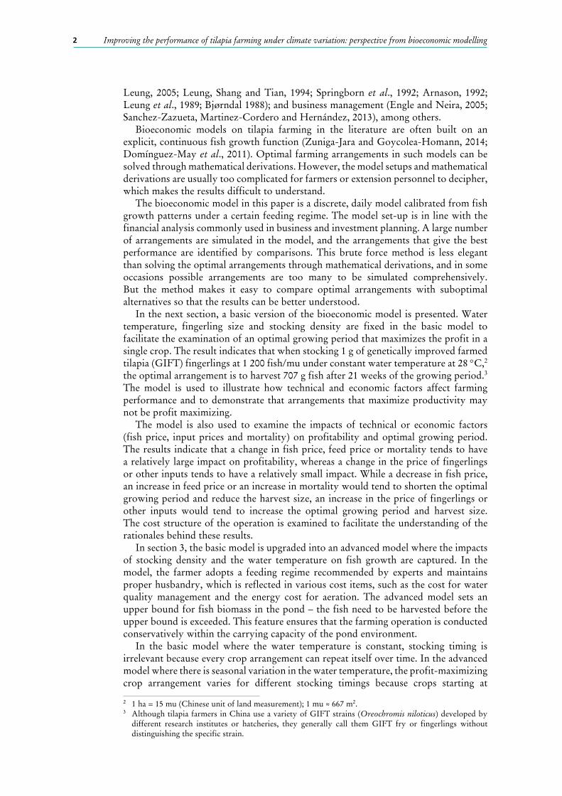
Original data on tilapia growthTable 1 shows a tilapia growth pattern published in a technical guidebook on tilapia farming in China, prepared by experts in the China Agriculture Research System for Tilapia (Yang, 2015, pp. 55–56). The growth pattern is calibrated from field experience, experimental data and the scientific literature and used in the guidebook as a benchmark feeding schedule.
The pattern represents a growth path of GIFT tilapia in pond aquaculture under constant water temperature at 28 °C, 1 g fingerlings, 1 200 fish/mu (i.e. 1.8 fish/m2; 1 ha = 15 mu) stocking density, and a specific feeding scheme. With daily feeding at 10 percent of the body weight, a 1 g fingerling would grow to 5 g after week 1; with daily feeding at 5 percent of the body weight, the 5 g fingerling would grow to 8 g after week 2, and so on.
Improving the performance of tilapia farming under climate variation: perspective from bioeconomic modelling6
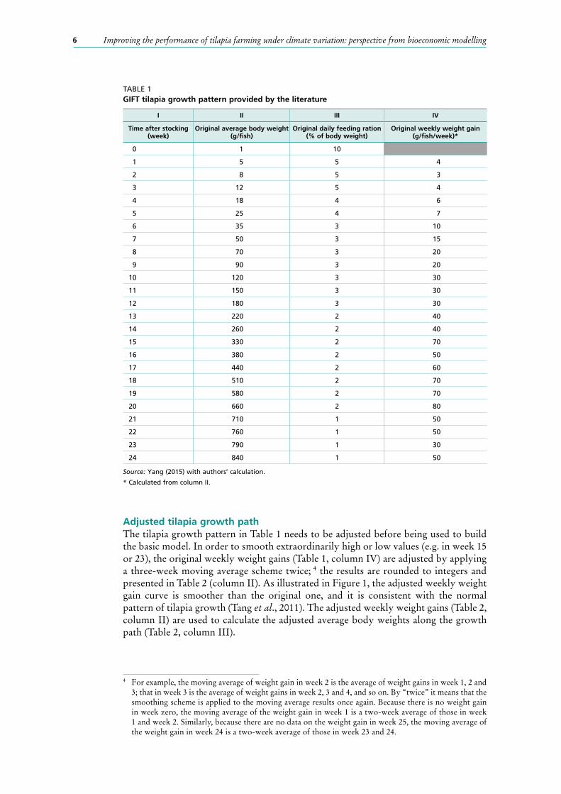
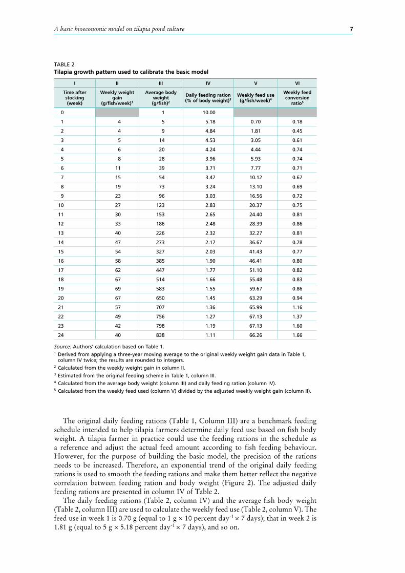
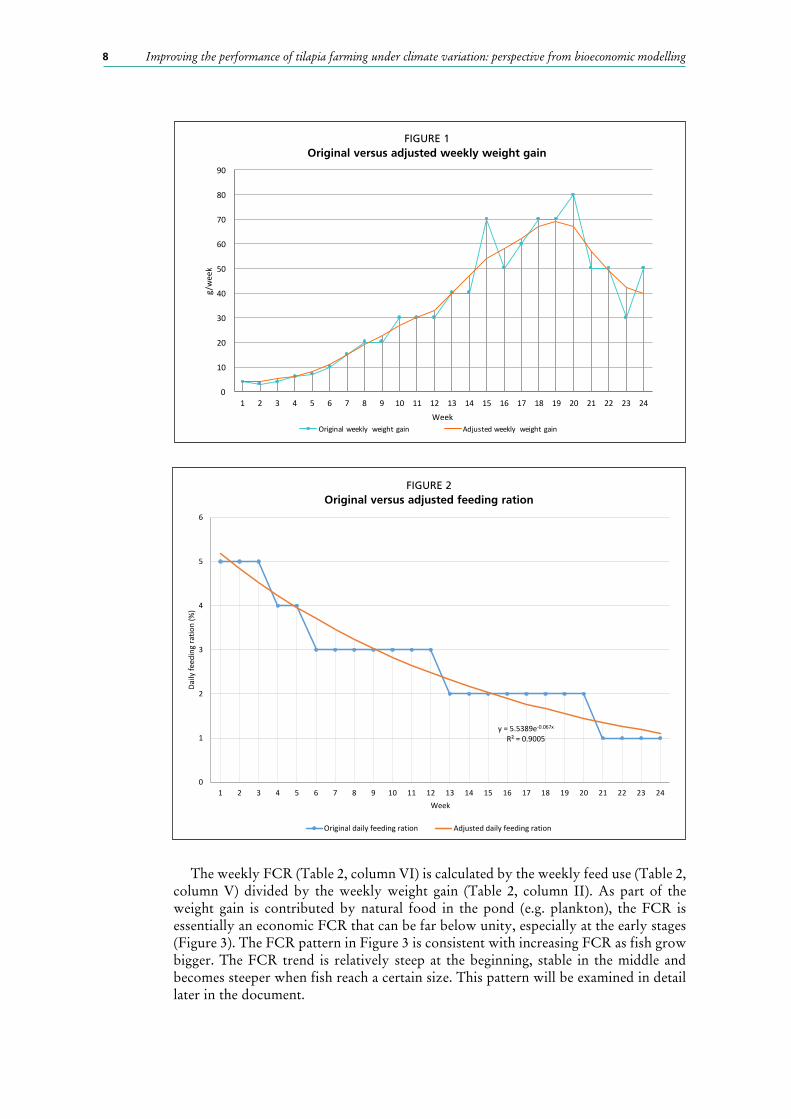
Adjusted tilapia growth pathThe tilapia growth pattern in Table 1 needs to be adjusted before being used to build the basic model. In order to smooth extraordinarily high or low values (e.g. in week 15 or 23), the original weekly weight gains (Table 1, column IV) are adjusted by applying a three-week moving average scheme twice; 4 the results are rounded to integers and presented in Table 2 (column II). As illustrated in Figure 1, the adjusted weekly weight gain curve is smoother than the original one, and it is consistent with the normal pattern of tilapia growth (Tang et al., 2011). The adjusted weekly weight gains (Table 2, column II) are used to calculate the adjusted average body weights along the growth path (Table 2, column III).
4 For example, the moving average of weight gain in week 2 is the average of weight gains in week 1, 2 and 3; that in week 3 is the average of weight gains in week 2, 3 and 4, and so on. By “twice” it means that the smoothing scheme is applied to the moving average results once again. Because there is no weight gain in week zero, the moving average of the weight gain in week 1 is a two-week average of those in week 1 and week 2. Similarly, because there are no data on the weight gain in week 25, the moving average of the weight gain in week 24 is a two-week average of those in week 23 and 24.
TABLE 1GIFT tilapia growth pattern provided by the literature
I II III IV
Time after stocking(week)
Original average body weight(g/fish)
Original daily feeding ration (% of body weight)
Original weekly weight gain(g/fish/week)*
0 1 10
1 5 5 4
2 8 5 3
3 12 5 4
4 18 4 6
5 25 4 7
6 35 3 10
7 50 3 15
8 70 3 20
9 90 3 20
10 120 3 30
11 150 3 30
12 180 3 30
13 220 2 40
14 260 2 40
15 330 2 70
16 380 2 50
17 440 2 60
18 510 2 70
19 580 2 70
20 660 2 80
21 710 1 50
22 760 1 50
23 790 1 30
24 840 1 50
Source: Yang (2015) with authors’ calculation.
* Calculated from column II.
7A basic bioeconomic model on tilapia pond culture
TABLE 2Tilapia growth pattern used to calibrate the basic model
I II III IV V VI
Time after stocking(week)
Weekly weight gain
(g/fish/week)1
Average body weight(g/fish)2
Daily feeding ration (% of body weight)3
Weekly feed use (g/fish/week)4
Weekly feed conversion
ratio5
0 1 10.00
1 4 5 5.18 0.70 0.18
2 4 9 4.84 1.81 0.45
3 5 14 4.53 3.05 0.61
4 6 20 4.24 4.44 0.74
5 8 28 3.96 5.93 0.74
6 11 39 3.71 7.77 0.71
7 15 54 3.47 10.12 0.67
8 19 73 3.24 13.10 0.69
9 23 96 3.03 16.56 0.72
10 27 123 2.83 20.37 0.75
11 30 153 2.65 24.40 0.81
12 33 186 2.48 28.39 0.86
13 40 226 2.32 32.27 0.81
14 47 273 2.17 36.67 0.78
15 54 327 2.03 41.43 0.77
16 58 385 1.90 46.41 0.80
17 62 447 1.77 51.10 0.82
18 67 514 1.66 55.48 0.83
19 69 583 1.55 59.67 0.86
20 67 650 1.45 63.29 0.94
21 57 707 1.36 65.99 1.16
22 49 756 1.27 67.13 1.37
23 42 798 1.19 67.13 1.60
24 40 838 1.11 66.26 1.66
Source: Authors’ calculation based on Table 1. 1 Derived from applying a three-year moving average to the original weekly weight gain data in Table 1,
column IV twice; the results are rounded to integers. 2 Calculated from the weekly weight gain in column II. 3 Estimated from the original feeding scheme in Table 1, column III. 4 Calculated from the average body weight (column III) and daily feeding ration (column IV). 5 Calculated from the weekly feed used (column V) divided by the adjusted weekly weight gain (column II).
The original daily feeding rations (Table 1, Column III) are a benchmark feeding schedule intended to help tilapia farmers determine daily feed use based on fish body weight. A tilapia farmer in practice could use the feeding rations in the schedule as a reference and adjust the actual feed amount according to fish feeding behaviour. However, for the purpose of building the basic model, the precision of the rations needs to be increased. Therefore, an exponential trend of the original daily feeding rations is used to smooth the feeding rations and make them better reflect the negative correlation between feeding ration and body weight (Figure 2). The adjusted daily feeding rations are presented in column IV of Table 2.
The daily feeding rations (Table 2, column IV) and the average fish body weight (Table 2, column III) are used to calculate the weekly feed use (Table 2, column V). The feed use in week 1 is 0.70 g (equal to 1 g × 10 percent day-1 × 7 days); that in week 2 is 1.81 g (equal to 5 g × 5.18 percent day-1 × 7 days), and so on.
Improving the performance of tilapia farming under climate variation: perspective from bioeconomic modelling8
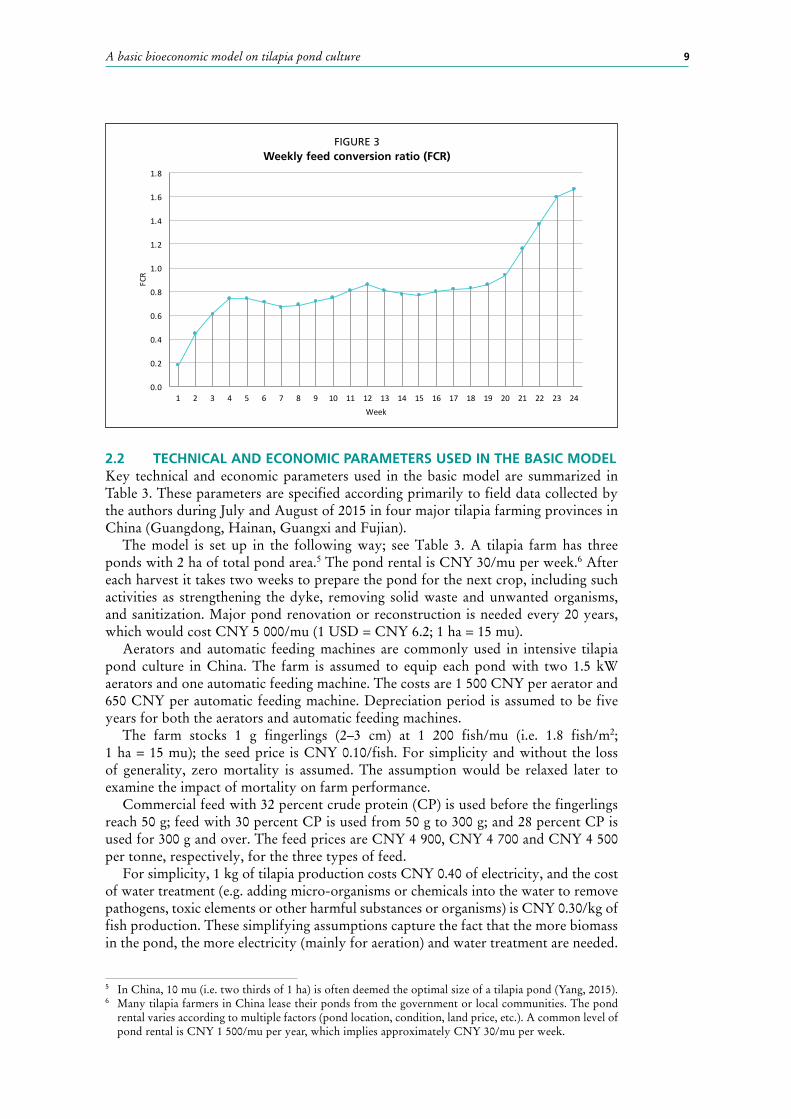
The weekly FCR (Table 2, column VI) is calculated by the weekly feed use (Table 2, column V) divided by the weekly weight gain (Table 2, column II). As part of the weight gain is contributed by natural food in the pond (e.g. plankton), the FCR is essentially an economic FCR that can be far below unity, especially at the early stages (Figure 3). The FCR pattern in Figure 3 is consistent with increasing FCR as fish grow bigger. The FCR trend is relatively steep at the beginning, stable in the middle and becomes steeper when fish reach a certain size. This pattern will be examined in detail later in the document.
0
10
20
30
40
50
60
70
80
90
1 2 3 4 5 6 7 8 9 10 11 12 13 14 15 16 17 18 19 20 21 22 23 24
g/week
WeekOriginalweekly weightgain Adjustedweekly weightgain
FIGURE 1Original versus adjusted weekly weight gain
y = 5.5389e-0.067x
R² = 0.9005
0
1
2
3
4
5
6
1 2 3 4 5 6 7 8 9 10 11 12 13 14 15 16 17 18 19 20 21 22 23 24
Daily
feed
ing
ratio
n (%
)
Week
Original daily feeding ration Adjusted daily feeding ration
FIGURE 2Original versus adjusted feeding ration
9A basic bioeconomic model on tilapia pond culture
2.2 TECHNICAL AND ECONOMIC PARAMETERS USED IN THE BASIC MODELKey technical and economic parameters used in the basic model are summarized in Table 3. These parameters are specified according primarily to field data collected by the authors during July and August of 2015 in four major tilapia farming provinces in China (Guangdong, Hainan, Guangxi and Fujian).
The model is set up in the following way; see Table 3. A tilapia farm has three ponds with 2 ha of total pond area.5 The pond rental is CNY 30/mu per week.6 After each harvest it takes two weeks to prepare the pond for the next crop, including such activities as strengthening the dyke, removing solid waste and unwanted organisms, and sanitization. Major pond renovation or reconstruction is needed every 20 years, which would cost CNY 5 000/mu (1 USD = CNY 6.2; 1 ha = 15 mu).
Aerators and automatic feeding machines are commonly used in intensive tilapia pond culture in China. The farm is assumed to equip each pond with two 1.5 kW aerators and one automatic feeding machine. The costs are 1 500 CNY per aerator and 650 CNY per automatic feeding machine. Depreciation period is assumed to be five years for both the aerators and automatic feeding machines.
The farm stocks 1 g fingerlings (2–3 cm) at 1 200 fish/mu (i.e. 1.8 fish/m2; 1 ha = 15 mu); the seed price is CNY 0.10/fish. For simplicity and without the loss of generality, zero mortality is assumed. The assumption would be relaxed later to examine the impact of mortality on farm performance.
Commercial feed with 32 percent crude protein (CP) is used before the fingerlings reach 50 g; feed with 30 percent CP is used from 50 g to 300 g; and 28 percent CP is used for 300 g and over. The feed prices are CNY 4 900, CNY 4 700 and CNY 4 500 per tonne, respectively, for the three types of feed.
For simplicity, 1 kg of tilapia production costs CNY 0.40 of electricity, and the cost of water treatment (e.g. adding micro-organisms or chemicals into the water to remove pathogens, toxic elements or other harmful substances or organisms) is CNY 0.30/kg of fish production. These simplifying assumptions capture the fact that the more biomass in the pond, the more electricity (mainly for aeration) and water treatment are needed.
5 In China, 10 mu (i.e. two thirds of 1 ha) is often deemed the optimal size of a tilapia pond (Yang, 2015). 6 Many tilapia farmers in China lease their ponds from the government or local communities. The pond
rental varies according to multiple factors (pond location, condition, land price, etc.). A common level of pond rental is CNY 1 500/mu per year, which implies approximately CNY 30/mu per week.
0.0
0.2
0.4
0.6
0.8
1.0
1.2
1.4
1.6
1.8
1 2 3 4 5 6 7 8 9 10 11 12 13 14 15 16 17 18 19 20 21 22 23 24
FCR
Week
FIGURE 3Weekly feed conversion ratio (FCR)

Improving the performance of tilapia farming under climate variation: perspective from bioeconomic modelling10
The farm hires one full-time worker who is paid CNY 650 per week. The farm outsources harvesting tasks to a professional harvest team, which would charge a lump sum of CNY 3 000.
In China, tilapia are available to consumers and the industry in various sizes. Tilapia smaller than 250 g are usually not marketable and are sold as juveniles at a very low price. Tilapia weighing less than 500 g are deemed a small-size fish and are usually cheaper than larger size tilapia. Fish processing plants prefer to collect tilapia that weigh more than 500 g. Tilapia weighing more than 1 kg are usually supplied to the food catering industry with a size premium in price. The farmgate tilapia prices specified in Table 3 capture these stylized facts.
2.3 ASSESSING THE PERFORMANCE OF TILAPIA POND CULTURE IN THE BASIC MODELThe biological component (Table 2) and the technical and economic parameters (Table 3) are combined into the basic bioeconomic model. A key feature of the basic
TABLE 3Technical and economic parameters used in the basic model
Pond
Area (ha) 2
Number of ponds 3
Pond rental (CNY/mu/week) 30
Time for pond preparation (weeks) 2
Pond renovation/reconstruction (every 20 years) (CNY/mu) 5 000
Equipment
Number of 1.5 kW aerators (number/pond) 2
Price of 1.5 kW aerator (CNY/aerator) 1 500
Depreciation period for aerator (year) 5
Automatic feeding machine (number/pond) 1
Price of automatic feeding machine (CNY/machine) 650
Depreciation period for automatic feeding machine (year) 5
Seed
Fingerling price (1 g, 2–3 cm) (CNY/fish) 0.10
Stocking density (fish/mu) 1 200
Mortality (%) -
Feed
Feed price (32 percent crude protein, used before 50 g) (CNY/tonne) 4 900
Feed price (30 percent crude protein, used from 50 to 300 g) (CNY/tonne) 4 700
Feed price (28 percent crude protein, used after 300 g) (CNY/tonne) 4 500
Electricity and water treatment
Electricity or other energy cost (CNY/kg of fish production) 0.40
Water treatment cost (CNY/kg of fish production) 0.30
Labour
Number of workers 1
Wage (CNY/week) 650
Harvest team (CNY/time) 3 000
Fish price
Farmgate tilapia price (< 250 g) (CNY/kg) 5.02
Farmgate tilapia price (> = 250 but < 500 g) (CNY/kg) 7.95
Farmgate tilapia price (> = 500 but < 1 000 g) (CNY/kg) 9.84
Farmgate tilapia price (> = 1 000 g) (CNY/kg) 11.40

11A basic bioeconomic model on tilapia pond culture
model is that the water temperature is assumed to be constant at 28 °C; the assumption would be relaxed in the advanced model.
In the basic model, most of the key farming arrangements or practices such as fingerling size, stocking density, feed choice and feeding regime are exogenously specified according to common practices in China. There is no need to specify stocking timing since the assumption of constant water temperature implies a uniform farming condition for any crop. Growing period (or crop length) is the only endogenous variable in the model, which is selected by the farmer to optimize the farming performance.
Table 4 shows the technical and economic performance of tilapia farming along the fish growth path in the basic model. For example, when harvesting the fish 21 weeks after stocking (Table 4, column I), the average harvest size would be 707 g (Table 4, column II). With 1 200 fish/m2 stocking density and zero mortality, the number of fish harvested would be 18 000/ha, which implies 12 726 kg/ha per crop of tilapia production (Table 4, column III, equal to 0.707 kg multiplied by 18 000) and 553 kg/ha per week (Table 4, column XII, equal to 12 726 kg/ha per crop ÷ 23 weeks/crop).7
With CNY 9.84/fish of farmgate tilapia price (Table 4, column V), the farm revenue would be CNY 125 181/ha per crop (Table 4, column VI, equal to 12 726 kg/ha per crop multiplied by CNY 9.84/kg).8
When harvesting in week 21, the fixed cost (Table 4, column VII) would be CNY 12 493/ha per crop, including CNY 10 350/ha per crop of pond rental, CNY 484/ha per crop of equipment depreciation, and CNY 1 659/ha per crop of the amortized cost of pond renovation/reconstruction incurred every 20 years.
• With CNY 30/mu weekly pond rental (Table 3), the pond rental cost would be CNY 10 350/ha per crop, equal to 30 CNY/mu per week × 15 mu/ha × 23 weeks/crop.9
• The two aerators and one automatic feeding machine cost CNY 10 950 (equal to CNY 1 500/aerator × two aerators/pond × three ponds + CNY 650/automatic feeding machine × one automatic feeding machine/pond × three ponds; see Table 3). Thus, the equipment depreciation would be CNY 484/ha per crop (equal to CNY 10 950 ÷ 5 years ÷ 52 weeks/year × 23 weeks/crop ÷ 2 ha).
• The pond renovation/reconstruction would cost CNY 5 000/mu (Table 3); thus, the amortization of this cost would be CNY 1 659/ha per crop (CNY 5 000/mu × 15 mu/ha ÷ 20 years ÷ 52 weeks/year × 23 weeks/crop).
When harvesting in week 21, the operating cost would be CNY 68 214/ha per crop (Table 4, column VIII), including CNY 1 800/ha per crop for seed, CNY 48 531/ha per crop for feed, CNY 5 090/ha per crop for electricity, CNY 3 818/ha per crop for water treatment, and CNY 8 975/ha per crop for labour.
• With the 1 200 fish/mu stocking density, the number of fish stocked is 18 000/ha per crop (equal to 1 200 fish/mu × 15 mu/ha), and the seed cost would be CNY 1 800/ha per crop (equal to 18 000 fish/ha per crop × CNY 0.10/fish), irrespective of the growing period.
• The CNY 48 531/ha per crop of feed cost is the sum of the cost of feed use in each week (Table 2, column V). For example, the feed use in week 21 is 1 187 826 g/ha (equal to 65.99 g/fish × 18 000 fish/ha). With the feed price (28 percent CP) of CNY 4 500/tonne (i.e. CNY 0.0045/g), the feed cost in week 21 would be CNY 5 345/ha (equal to 1 187 826 g/ha × CNY 0.0045/g).
• The production of 1 kg tilapia would cost CNY 0.40 for electricity and CNY 0.30 for water treatment (Table 3). Thus, the production of 12 726 kg/ha per crop would cost CNY 5 090/ha per crop and CNY 3 818/ha per crop for the use of electricity and water treatments, respectively.
7 The crop length of 23 weeks includes the growth period (21 weeks) plus two weeks for pond preparation.8 Discrepancy may occur from rounding – the price CNY 9.84 is the rounding of CNY 9.83667.9 1 ha = 15 mu.

Improving the performance of tilapia farming under climate variation: perspective from bioeconomic modelling12
• The wage for the full-time worker comes out to be CNY 14 950 (equal to CNY 650/week × 23 weeks), and hiring the harvest team would cost CNY 3 000 (Table 3). Therefore, the (internal and external) labour cost would be CNY 8 975/ha per crop (equal to (CNY 14 950/crop + CNY 3 000/crop) ÷ 2 ha).
With the CNY 125 181/ha per crop of revenue and CNY 80 707/ha per crop of total cost (Table 4, column IX, equal to the CNY 12 493/ha per crop of fixed cost plus the CNY 68 214/ha per crop of operating cost), the profit (equal to revenue minus cost) from harvesting in week 21 would be CNY 44 475/ha per crop (Table 4, column X) and CNY 1 934/ha per week (Table 4, column XI). The break-even price (Table 4, column XIII) shows that when harvesting in week 21, farmers would be able to break even (i.e. zero profit) by selling fish at CNY 6.34/kg, which would generate revenue just enough to cover the total cost. In other words, a farmer would be able to make money by selling the fish at a price higher than CNY 6.34/kg.
Profit per crop Profit per crop, which is equal to revenue per crop minus cost per crop, is a common indicator for measuring the economic performance of an aquaculture operation. As indicated in Table 4 and Figure 4, the farmer would lose money (i.e. negative profit per crop) if the fish are harvested before week 14. The low price for undersized fish – i.e. CNY 5.02/fish for fish weighing less than 250 g – is the primary cause of this situation.
As shown in Figure 4, the loss would be increasing with the growth period before week 14. For example, harvesting the fish at 186 g in week 12 would incur less loss than harvesting the fish at 226 g in week 13. This indicates the importance of growing fish to a marketable size. Similarly, profit per crop would have a big jump in week 18 when the fish exceed 500 g and can be sold at a higher price.
From week 18 to week 24, profit per crop would be increasing with the length of the growing period. This means that harvesting the fish in week 24 would yield greater profit per crop than harvesting the fish earlier. However, is harvesting in week 24 the optimal arrangement? The answer is negative.
Although harvesting in week 24 would yield a higher profit per crop than harvesting in week 23 (CNY 47 713/ha per crop versus CNY 46 830/ha crop), it would also take up one more week of production. Generally speaking, profit per crop is not an accurate indicator for comparing the profitability of production cycles with different crop
-20000
0
20000
40000
60000
80000
100000
120000
140000
160000
1 2 3 4 5 6 7 8 9 10 11 12 13 14 15 16 17 18 19 20 21 22 23 24
CNY/ha/crop
Growing period (weeks)Revenue percrop Cost percrop Profit percrop
FIGURE 4Profit per crop for different growth periods

13A basic bioeconomic model on tilapia pond culture
TAB
LE 4
Tech
nic
al a
nd
eco
no
mic
per
form
ance
of
inte
nsi
ve t
ilap
ia p
on
d c
ult
ure
in t
he
bas
ic m
od
el
III
IIIIV
VV
IV
IIV
IIIIX
XX
IX
IIX
III
Gro
win
g
per
iod
(wee
ks)
Fish
siz
e (g
/fis
h)
Pro
du
ctio
n
per
cro
p(k
g/h
a/cr
op
)FC
RPr
ice
(CN
Y/k
g)
Rev
enu
e p
er c
rop
(CN
Y/h
a/cr
op
)
Co
st p
er c
rop
(C
NY
/ha/
cro
p)
Key
per
form
ance
ind
icat
ors
Fixe
d
cost
Op
erat
ing
co
stTo
tal c
ost
Pro
fit
per
cro
p
(CN
Y/h
a/cr
op
)Pr
ofi
t p
er w
eek
(CN
Y/h
a/w
eek)
Pro
du
ctio
n p
er w
eek
(kg
/ha/
wee
k)B
reak
-eve
n p
rice
(C
NY
/kg
)
1 5
90
0.18
5.02
4
511
630
4 40
06
029
-5 5
78-1
859
30
66.9
9
2 9
162
0.45
5.02
8
132
173
4 93
57
108
-6 2
95-1
574
41
43.8
7
3 1
4 2
520.
61
5.
02
1 26
42
716
5 59
28
308
-7 0
44-1
409
50
32.9
7
4 2
0 3
600.
74
5.
02
1 80
63
259
6 38
49
643
-7 8
38-1
306
60
26.7
9
5 2
8 5
040.
74
5.
02
2 52
83
802
7 33
311
136
-8 6
08-1
230
72
22.0
9
6 3
9 7
020.
71
5.
02
3 52
14
345
8 48
212
827
-9 3
06-1
163
88
18.2
7
7 5
4 9
720.
67
5
.02
4 87
54
889
9 85
214
740
-9 8
65-1
096
108
15.1
6
8 7
31
314
0.69
5.02
6
591
5 43
211
524
16 9
56-1
0 36
5-1
037
131
12.9
9 9
61
728
0.72
5.02
8
667
5 97
513
540
19 5
15-1
0 84
8-
986
157
11.2
9
10 1
232
214
0.75
5.02
11
105
6 51
815
928
22 4
46-1
1 34
1-
945
185
10.1
4
11 1
532
754
0.81
5.02
13
814
7 06
118
696
25 7
57-1
1 94
3-
919
212
9.35
12 1
863
348
0.86
5.02
16
793
7 60
421
838
29 4
43-1
2 65
0-
904
239
8.79
13 2
264
068
0.81
5.0
2 20
404
8 14
825
398
33 5
45-1
3 14
1-
876
271
8.25
14 2
734
914
0.78
7.9
5 39
048
8 69
129
417
38 1
08 9
40 5
9 3
077.
76
15 3
275
886
0.77
7.9
5 46
772
9 23
433
779
43 0
133
759
221
346
7.31
16 3
856
930
0.80
7.9
5 55
068
9 77
738
594
48 3
716
697
372
385
6.98
17 4
478
046
0.82
7.9
5 63
936
10 3
2043
839
54 1
599
776
515
423
6.73
18 5
149
252
0.83
9.84
91
009
10 8
6349
502
60 3
6630
643
1 53
2 4
636.
52
19 5
8310
494
0.86
9.84
10
3 22
611
407
55 5
3066
936
36 2
901
728
500
6.38
20 6
5011
700
0.94
9.84
11
5 08
911
950
61 8
2573
775
41 3
141
878
532
6.31
21 7
0712
726
1.16
9
.84
125
181
12 4
9368
214
80 7
0744
475
1 93
4 5
536.
34
22 7
5613
608
1.37
9.8
4 13
3 85
713
036
74 5
9387
629
46 2
281
926
567
6.44
23 7
9814
364
1.60
9.84
14
1 29
413
579
80 8
8594
464
46 8
301
873
575
6.58
24 8
3815
084
1.66
9
.84
148
376
14 1
2387
081
101
204
47 1
731
814
580
6.71
Improving the performance of tilapia farming under climate variation: perspective from bioeconomic modelling14
length; indicators with uniform crop length, such as profit per week, profit per month or profit per year, should be used instead.
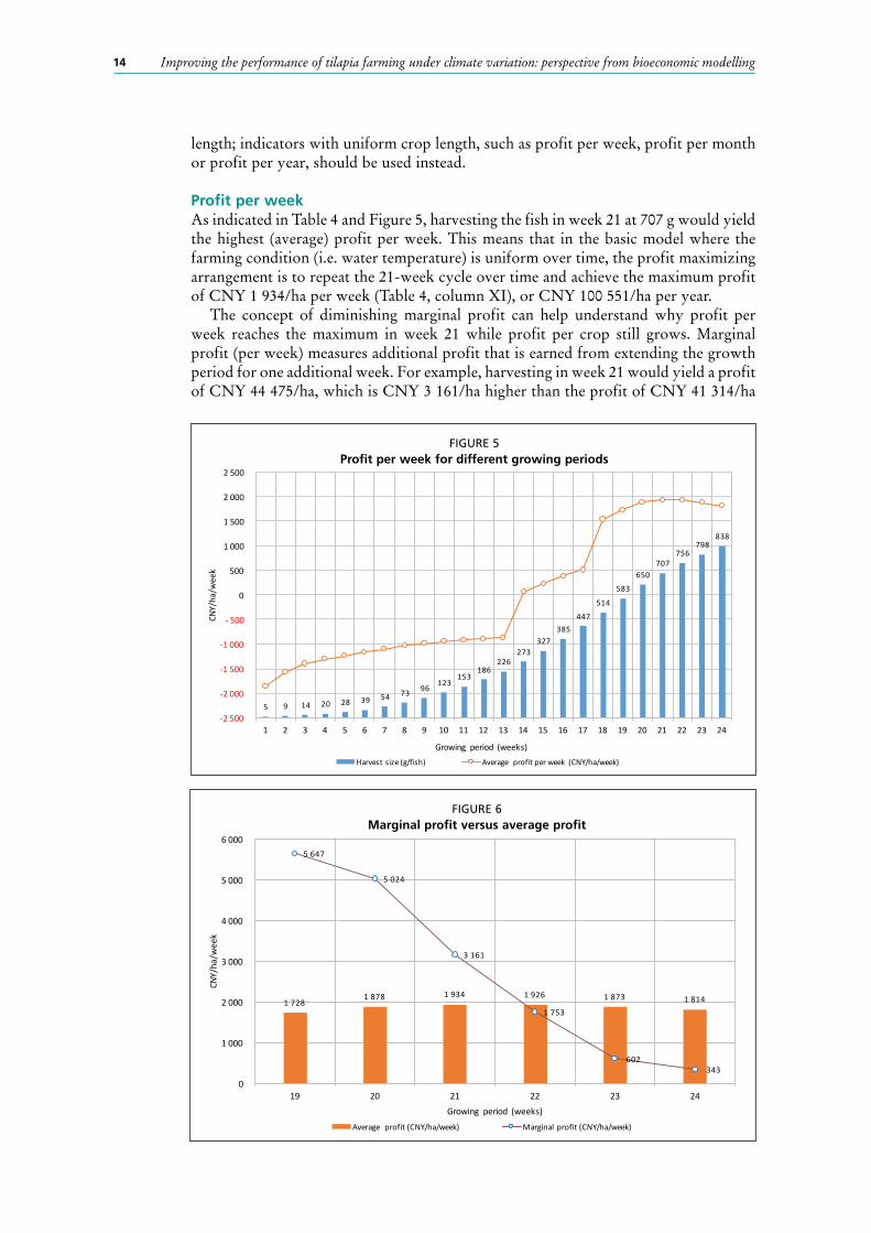
Profit per weekAs indicated in Table 4 and Figure 5, harvesting the fish in week 21 at 707 g would yield the highest (average) profit per week. This means that in the basic model where the farming condition (i.e. water temperature) is uniform over time, the profit maximizing arrangement is to repeat the 21-week cycle over time and achieve the maximum profit of CNY 1 934/ha per week (Table 4, column XI), or CNY 100 551/ha per year.
The concept of diminishing marginal profit can help understand why profit per week reaches the maximum in week 21 while profit per crop still grows. Marginal profit (per week) measures additional profit that is earned from extending the growth period for one additional week. For example, harvesting in week 21 would yield a profit of CNY 44 475/ha, which is CNY 3 161/ha higher than the profit of CNY 41 314/ha
5 9 14 20 28 39 54 73 96123
153186
226273
327385
447
514
583
650707
756798
838
-2500
-2000
-1500
-1000
- 500
0
500
1000
1500
2000
2500
1 2 3 4 5 6 7 8 9 10 11 12 13 14 15 16 17 18 19 20 21 22 23 24
CNY/ha/w
eek
Growing period (weeks)Harvest size(g/fish) Average profitperweek (CNY/ha/week)
FIGURE 5Profit per week for different growing periods
17281878 1934 1926 1873 1814
5647
5024
3161
1753
602343
0
1000
2000
3000
4000
5000
6000
19 20 21 22 23 24
CNY/ha/w
eek
Growing period (weeks)Average profit(CNY/ha/week) Marginalprofit(CNY/ha/week)
FIGURE 6Marginal profit versus average profit

15A basic bioeconomic model on tilapia pond culture
from harvesting in week 20. Thus, the marginal profit in week 21 is CNY 3 161/ha per week. As shown in Figure 6, marginal profit diminishes from CNY 5 647/ha per week in week 19 to CNY 343/ha per week in week 24.
As the marginal profit in week 21 (CNY 3 161/ha per week) is higher than the average profit per week from harvesting in week 20 (CNY 1 878/ha per week), extending the growing period from 20 weeks to 21 weeks would increase the average profit per week; hence, harvesting in week 21 would be more profitable than in week 20.
As the marginal profit in week 22 (CNY 1 753/ha per week) is smaller than the average profit per week in week 21 (CNY 1 934/ha per week), extending the growth period from 21 weeks to 22 weeks would reduce the average profit per week; hence, harvesting in week 22 would be less profitable than in week 21. The diminishing marginal profit would continue to reduce the average profit per week in weeks 23 and 24. Therefore, the most profitable option is harvesting in week 21.
Marginal profit is equal to marginal revenue minus marginal cost. The primary cause of the diminishing marginal profit (Figure 6) is the diminishing marginal revenue from 12 217 CNY/ha per week in week 19 to CNY 7 082/ha per week in week 24, which is, in turn, caused by diminishing marginal production (Figure 7). As fish grow bigger and bigger, the increasing fish biomass would put increasing pressure on the carrying capacity of the ponds (natural food, oxygen, etc.). In addition, larger fish would need more energy to sustain their metabolism. Therefore, when the biomass in the pond reaches a certain threshold, the weekly weight gain of fish would start to decline (Figure 1), which would lead to diminishing marginal production.
As indicated in Figure 7, marginal cost increases slightly from CNY 6 571/ha per week in week 19 to CNY 6 932/ha per week in week 21. This is a contributing factor to the diminishing marginal profit, yet the magnitude is far less than the impact of the diminishing marginal revenue. Indeed, the marginal cost peaks at week 21 and declines until week 24, which serves as a countering factor to the diminishing marginal profit. There will be a more detailed discussion on cost later in the document.
Technical performance versus economic performanceAs indicated in Table 4, profit per week peaks in week 21 (column XI), whereas production per week (column XII) keeps growing to the end of the planning horizon (i.e. week 24). As shown in Figure 8, although marginal production peaks in week 19
1242 12061026
882756 720
1221711863
10092
8676
74377082
65716839 6932 6923 6835 6740
19 20 21 22 23 24Growing period (weeks)
Marginalproduction(kg/ha/week) Marginal revenue (CNY/ha/week) Marginal cost(CNY/ha/week)
FIGURE 7Marginal revenue and marginal cost
Improving the performance of tilapia farming under climate variation: perspective from bioeconomic modelling16
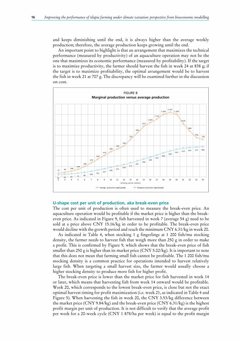
and keeps diminishing until the end, it is always higher than the average weekly production; therefore, the average production keeps growing until the end.
An important point to highlight is that an arrangement that maximizes the technical performance (measured by productivity) of an aquaculture operation may not be the one that maximizes its economic performance (measured by profitability). If the target is to maximize productivity, the farmer should harvest the fish in week 24 at 838 g; if the target is to maximize profitability, the optimal arrangement would be to harvest the fish in week 21 at 707 g. The discrepancy will be examined further in the discussion on cost.
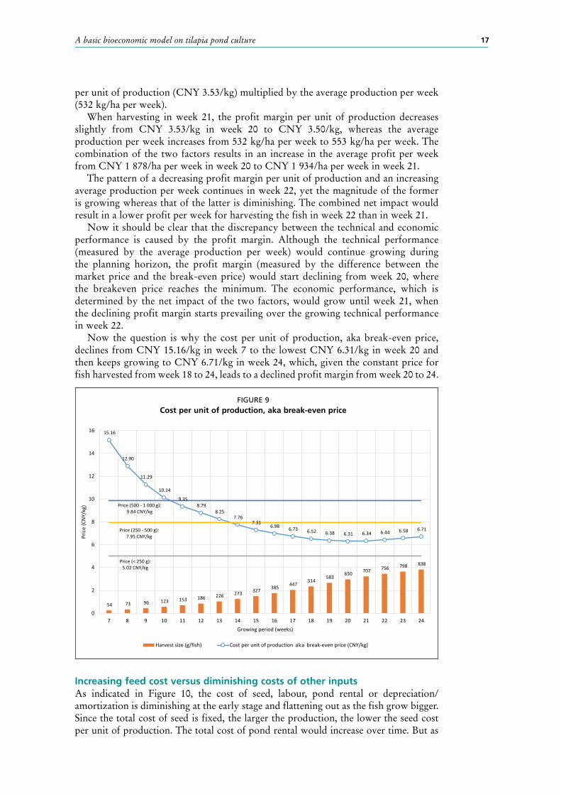
U-shape cost per unit of production, aka break-even priceThe cost per unit of production is often used to measure the break-even price. An aquaculture operation would be profitable if the market price is higher than the break-even price. As indicated in Figure 9, fish harvested in week 7 (average 54 g) need to be sold at a price above CNY 15.16/kg in order to be profitable. The break-even price would decline with the growth period and reach the minimum CNY 6.31/kg in week 20.
As indicated in Table 4, when stocking 1 g fingerlings at 1 200 fish/mu stocking density, the farmer needs to harvest fish that weigh more than 250 g in order to make a profit. This is confirmed by Figure 9, which shows that the break-even price of fish smaller than 250 g is higher than its market price (CNY 5.02/kg). It is important to note that this does not mean that farming small fish cannot be profitable. The 1 200 fish/mu stocking density is a common practice for operations intended to harvest relatively large fish. When targeting a small harvest size, the farmer would usually choose a higher stocking density to produce more fish for higher profit.
The break-even price is lower than the market price for fish harvested in week 14 or later, which means that harvesting fish from week 14 onward would be profitable. Week 20, which corresponds to the lowest break-even price, is close but not the exact optimal harvest timing for profit maximization (i.e. week 21, as indicated in Table 4 and Figure 5). When harvesting the fish in week 20, the CNY 3.53/kg difference between the market price (CNY 9.84/kg) and the break-even price (CNY 6.31/kg) is the highest profit margin per unit of production. It is not difficult to verify that the average profit per week for a 20-week cycle (CNY 1 878/ha per week) is equal to the profit margin
41 50 60 72 88 108131
157185
212239
271307
346385
423463
500532 553 567 575 580
72 90 108144
198
270
342
414
486540
594
720
846
972
1044
1116
12061242
1206
1026
882
756720
2 3 4 5 6 7 8 9 10 11 12 13 14 15 16 17 18 19 20 21 22 23 24Growingperiod (weeks)
Average production(kg/ha/week) Marginalproduction(kg/ha/week)
FIGURE 8Marginal production versus average production
17A basic bioeconomic model on tilapia pond culture
per unit of production (CNY 3.53/kg) multiplied by the average production per week (532 kg/ha per week).
When harvesting in week 21, the profit margin per unit of production decreases slightly from CNY 3.53/kg in week 20 to CNY 3.50/kg, whereas the average production per week increases from 532 kg/ha per week to 553 kg/ha per week. The combination of the two factors results in an increase in the average profit per week from CNY 1 878/ha per week in week 20 to CNY 1 934/ha per week in week 21.
The pattern of a decreasing profit margin per unit of production and an increasing average production per week continues in week 22, yet the magnitude of the former is growing whereas that of the latter is diminishing. The combined net impact would result in a lower profit per week for harvesting the fish in week 22 than in week 21.
Now it should be clear that the discrepancy between the technical and economic performance is caused by the profit margin. Although the technical performance (measured by the average production per week) would continue growing during the planning horizon, the profit margin (measured by the difference between the market price and the break-even price) would start declining from week 20, where the breakeven price reaches the minimum. The economic performance, which is determined by the net impact of the two factors, would grow until week 21, when the declining profit margin starts prevailing over the growing technical performance in week 22.
Now the question is why the cost per unit of production, aka break-even price, declines from CNY 15.16/kg in week 7 to the lowest CNY 6.31/kg in week 20 and then keeps growing to CNY 6.71/kg in week 24, which, given the constant price for fish harvested from week 18 to 24, leads to a declined profit margin from week 20 to 24.
Increasing feed cost versus diminishing costs of other inputsAs indicated in Figure 10, the cost of seed, labour, pond rental or depreciation/amortization is diminishing at the early stage and flattening out as the fish grow bigger. Since the total cost of seed is fixed, the larger the production, the lower the seed cost per unit of production. The total cost of pond rental would increase over time. But as
54 73 96 123 153 186 226 273 327 385 447 514
583 650 707 756 798 838
15.16
12.90
11.29
10.14
9.35 8.79
8.25 7.76
7.31 6.98 6.73 6.52 6.38 6.31 6.34 6.44 6.58 6.71
Price (< 250 g):5.02 CNY/kg
Price (250 - 500 g):7.95 CNY/kg
Price (500 - 1 000 g):9.84 CNY/kg
0
2
4
6
8
10
12
14
16
7 8 9 10 11 12 13 14 15 16 17 18 19 20 21 22 23 24
Price
(CNY
/kg)
Growing period (weeks)
Harvest size (g/fish) Cost per unit of production a.k.a break-even price (CNY/kg)
FIGURE 9Cost per unit of production, aka break-even price
aka
Improving the performance of tilapia farming under climate variation: perspective from bioeconomic modelling18
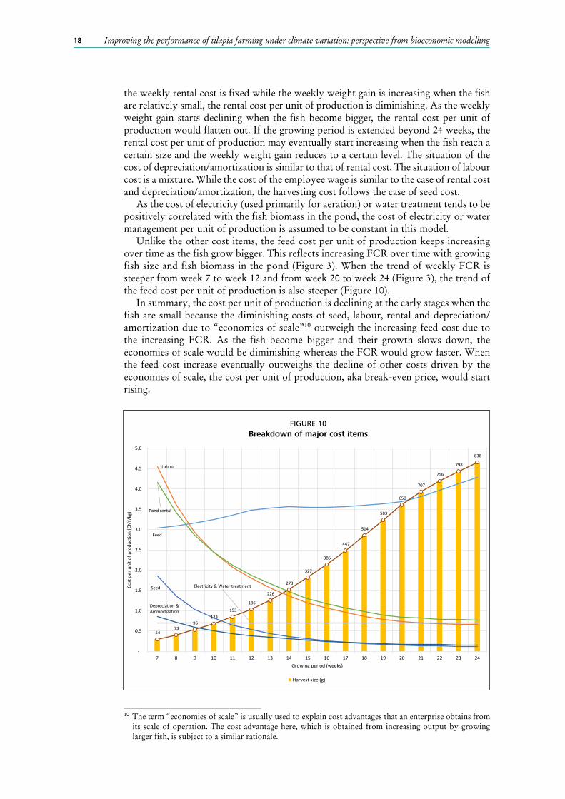
the weekly rental cost is fixed while the weekly weight gain is increasing when the fish are relatively small, the rental cost per unit of production is diminishing. As the weekly weight gain starts declining when the fish become bigger, the rental cost per unit of production would flatten out. If the growing period is extended beyond 24 weeks, the rental cost per unit of production may eventually start increasing when the fish reach a certain size and the weekly weight gain reduces to a certain level. The situation of the cost of depreciation/amortization is similar to that of rental cost. The situation of labour cost is a mixture. While the cost of the employee wage is similar to the case of rental cost and depreciation/amortization, the harvesting cost follows the case of seed cost.
As the cost of electricity (used primarily for aeration) or water treatment tends to be positively correlated with the fish biomass in the pond, the cost of electricity or water management per unit of production is assumed to be constant in this model.
Unlike the other cost items, the feed cost per unit of production keeps increasing over time as the fish grow bigger. This reflects increasing FCR over time with growing fish size and fish biomass in the pond (Figure 3). When the trend of weekly FCR is steeper from week 7 to week 12 and from week 20 to week 24 (Figure 3), the trend of the feed cost per unit of production is also steeper (Figure 10).
In summary, the cost per unit of production is declining at the early stages when the fish are small because the diminishing costs of seed, labour, rental and depreciation/amortization due to “economies of scale”10 outweigh the increasing feed cost due to the increasing FCR. As the fish become bigger and their growth slows down, the economies of scale would be diminishing whereas the FCR would grow faster. When the feed cost increase eventually outweighs the decline of other costs driven by the economies of scale, the cost per unit of production, aka break-even price, would start rising.
10 The term “economies of scale” is usually used to explain cost advantages that an enterprise obtains from its scale of operation. The cost advantage here, which is obtained from increasing output by growing larger fish, is subject to a similar rationale.
Feed
Seed
Labour
Electricity & Water treatment
Pond rental
Depreciation & Ammortization
54 73
96 123
153 186
226
273
327
385
447
514
583
650
707
756
798
838
-
0.5
1.0
1.5
2.0
2.5
3.0
3.5
4.0
4.5
5.0
7 8 9 10 11 12 13 14 15 16 17 18 19 20 21 22 23 24
Cost
per
uni
t of p
rodu
ctio
n (C
NY/k
g)
Growing period (weeks)
Harvest size (g)
FIGURE 10Breakdown of major cost items

19A basic bioeconomic model on tilapia pond culture
Cost structure The common perception that feed accounts for most of the cost of tilapia farming is confirmed in Figure 11, which indicates that when harvesting in week 21 (the optimal harvest timing), feed accounts for 60 percent of the total cost. However, the share of feed or any other cost item in the total cost depends on the growing period. When the fish are harvested in week 10 with the harvest size being 123 g, feed accounts for only a little over 30 percent of the total cost.
When the fish are harvested in week 21, pond rental and labour are two relatively large cost items, accounting for 12.8 and 11.1 percent of the total cost, respectively. They would be greater than the feed cost if the fish are harvested before week 9 (Figure 11). The share of pond rental is increasing in the early stage because the seed or labour cost, which is a lump-sum expense or has a lump-sum component (i.e. the harvesting expense), has greater “economies of scale” hence declines more rapidly than the pond rental. As the feed cost grows bigger, all three start declining and yield their shares in the total cost to the feed cost.
Seed is a relatively large cost item at the beginning, but becomes the smallest cost item, accounting for only 2.2 percent of the total cost when harvesting in week 21.
Impacts of technical or economic factors on profitability Table 5 shows how a technical or economic factor affects the profitability and optimal harvest time. The benchmark profitability in column V represents the situation presented in Table 4. Columns VI to X show the impacts on profitability (measured by profit per week) caused by a change in an input price, whereas column XI shows the impacts of a change in the fish price. It is assumed that the input or output price change would not alter the farmers’ stocking or feeding behaviours and hence does not affect the fish growth pattern (column II) or the technical performance of the operation (columns III and IV).
Recall that the benchmark case in Table 4 assumes zero fish mortality. The last four columns (columns XII to XV) in Table 5 depict a case of the weekly fish mortality being 2 percent. With the 2 percent weekly mortality, there would be 98 percent of fish survived at the end of week 1, then 96 percent (equal to 98 percent to the power 2) survived at the end of week 2, then 94 percent (equal to 98 percent to the power 3)
5 9 14 20 28 39 54 73
96 123
153 186
226
273
327
385
447
514
583
650
707
756
798 838 Feed, 60.1
Seed, 29.9
Seed, 2.2
Labour, 41.0
Labour, 11.1
Electricity, 6.3
Water management, 4.7
Pond rental, 28.3
Pond rental, 12.8
Depreciation & Ammortization, 2.7
0
5
10
15
20
25
30
35
40
45
50
55
60
65
70
1 2 3 4 5 6 7 8 9 10 11 12 13 14 15 16 17 18 19 20 21 22 23 24
Shar
e of
tota
l cos
t (%
)
Growing period (weeks)
Harvest size (g)
FIGURE 11Cost structure

Improving the performance of tilapia farming under climate variation: perspective from bioeconomic modelling20
survived at the end of week 3, and so on.11 The corresponding mortality rates (equal to one minus the survival rate) are presented in column XII. Unlike an economic factor affecting the profitability through an input or output price, the change in fish mortality (as a technical factor) would affect the profitability (column XV) through its impacts on fish production (columns XIII and XIV).
The impacts of the economic and technical factors on profitability are summarized as follows.
• As a minor cost accounting for only 2.2 percent of the total cost when the fish are harvested in week 21 (Figure 11), a change in the seed price would have a very small impact on the profitability. Indeed, a 50 percent increase in the fingerling price would only reduce the profitability by 2 percent from the benchmark level (CNY 1 934/ha per week) to 1 895 CNY/ha per week (Table 5, column VII). The optimal growing period is the same as that in the benchmark case (i.e. harvesting 707 g fish in week 21). However, if the fingerling price is increased by five times, the optimal growing period would be increased to 22 weeks and harvest size increased to 756 g. Intuitively, the more expensive the seed is, the more the “economies of scale” can be reaped by harvesting bigger fish.
• A 50 percent increase in the wage rate would reduce profitability by 10 percent from the benchmark level to CNY 1 739/ha per week (Table 5, column VIII). The impact is greater than seed, which reflects the higher share of labour cost than seed cost (Figure 11). Similar to the case of fingerlings, a five-time increase in wage rate would move the optimal harvest timing to week 22 (756 g). Similarly, a 50 percent increase in the electricity and water treatment cost would reduce the profitability by 10 percent to CNY 1 740/ha per week (Table 5, column IX), and a 50 percent increase in pond rental would reduce the profitability by 12 percent to CNY 1 709/ha per week (Table 5, column X).
• Being the largest cost item, a 50 percent increase in feed price would reduce the profitability by 54 percent to CNY 896/ha per week (Table 5, column VI). As opposed to an increase in the price of a cost that diminishes over time would increase the optimal growing period, the increase in the price of feed, which is a cost item increasing over time, would shorten the optimal growing period to 20 weeks and reduce the optimal harvest size to 650 g.
• A 30 percent decrease in fish price would reduce profitability by 84 percent to CNY 309/ha per week (Table 5, column XI). The lowered price reduces the profit margin per unit of production and hence would shorten the optimal growing period to 20 weeks and reduce the optimal harvest size to 650 g.
• An increase of weekly mortality from zero to 2 percent would reduce the profitability by 62 percent to 736 CNY/ha per week (Table 5, column XV). Mortality can be deemed a cost similar to feed which increases with the growing period. Therefore, the increased mortality would shorten the optimal growing period to 20 weeks and reduce the optimal harvest size to 650 g.
• In the last three cases, i.e. the 50 percent increase in feed price (Table 5, column VI), the 30 percent decrease in fish price (Table 5, column XI), and the increase of mortality from zero to 2 percent (Table 5, column XV), harvesting fish under 500 g would not be profitable given the relatively low prices for small-size fish.
SummaryA basic bioeconomic model has been developed based on the experience of intensive tilapia pond culture in China. The biological part of the model is based on the growth pattern of GIFT tilapia in China under specific farming conditions and practices,
11 This is a simplifying assumption, whereas in reality mortality tends to vary at different stages of fish growth.

21A basic bioeconomic model on tilapia pond culture
TAB
LE 5
Imp
act
of
tech
nic
al o
r ec
on
om
ic f
acto
rs o
n p
rofi
tab
ility
an
d o
pti
mal
har
vest
tim
e
III
IIIIV
VV
IV
IIV
IIIIX
XX
IX
IIX
IIIX
IVX
V
Gro
win
g
per
iod
(wee
ks)
Ave
rage
ha
rves
ting
size
(g/f
ish)
Pro
duct
ion
Prof
itabi
lity
(CNY
/ha/
wee
k) W
eekl
y m
orta
lity
2%
Kg/h
a/cr
op
Kg/h
a/w
eek
Benc
hmar
k Fe
ed p
rice
up
50%
Fi
nger
ling
price
up
50%
W
age
rate
up
50%
Elec
trici
ty &
wat
er
man
agem
ent p
rice
up 5
0%
Pond
rent
al
up 5
0%
Fish
pric
e do
wn
30%
Accu
mul
ated
m
orta
lity
(%)
Prod
uctio
n pe
r cro
p(k
g/ha
/cro
p)
Prod
uctiv
ity(k
g/ha
/wee
k)
Prof
itabi
lity
(CNY
/ha/
wee
k)
1
5
90
30
-1 8
59
-1 8
70
-2 1
59
-2 2
72
-1 8
70
-2 0
84
-1 9
04
2
88
29
-1 8
62
2
9
162
41
-1 5
74
-1 6
01
-1 7
99
-1 9
24
-1 5
88
-1 7
99
-1 6
35
4
156
3
9 -1
580
3
14
252
50
-1 4
09
-1 4
58
-1 5
89
-1 7
21
-1 4
26
-1 6
34
-1 4
85
6
237
4
7 -1
419
4
20
360
60
-1 3
06
-1 3
80
-1 4
56
-1 5
94
-1 3
27
-1 5
31
-1 3
97
8
332
5
5 -1
320
5
28
504
72
-1 2
30
-1 3
30
-1 3
58
-1 4
99
-1 2
55
-1 4
55
-1 3
38
10
456
6
5 -1
248
6
39
702
88
-1 1
63
-1 2
94
-1 2
76
-1 4
20
-1 1
94
-1 3
88
-1 2
95
11
622
7
8 -1
189
7
54
972
108
-1 0
96
-1 2
60
-1 1
96
-1 3
42
-1 1
34
-1 3
21
-1 2
59
13
844
9
4 -1
131
8
73
1 31
4 1
31-1
037
-1
239
-1
127
-1
274
-1
083
-1
262
-1
234
1
5 1
118
112
-1
082
9
96
1 72
8 1
57-
986
-1 2
34
-1 0
68
-1 2
17
-1 0
41
-1 2
11
-1 2
23
17
1 44
1 1
31
-1 0
45
10
123
2
214
185
- 94
5 -1
244
-1
020
-1
170
-1
010
-1
170
-1
223
1
8 1
809
151
-1
017
11
153
2
754
212
- 91
9 -1
274
-
988
-1 1
39
- 99
3 -1
144
-1
237
2
0 2
205
170
-1
004
12
186
3
348
239
- 90
4 -1
319
-
968
-1 1
20
- 98
7 -1
129
-1
263
2
2 2
627
188
-1
002
13
226
4
068
271
- 87
6 -1
355
-
936
-1 0
89
- 97
1 -1
101
-1
284
2
3 3
128
209
-
991
14
273
4
914
307
59
- 48
7 2
-
151
- 49
-
166
- 67
3 2
5 3
703
231
-
299
15
327
5
886
346
221
-
392
168
1
4 1
00
- 4
- 60
4 2
6 4
347
256
-
207
16
385
6
930
385
372
-
311
322
1
68
237
1
47
- 54
6 2
8 5
016
279
-
129
17
447
8
046
423
515
-
242
467
3
13
366
2
90
- 49
5 2
9 5
707
300
-
62
18
514
9
252
463
1 53
2 7
02
1 48
7 1
332
1 37
0 1
307
167
3
0 6
431
322
6
09
19
583
10
494
500
1 72
8 8
22
1 68
5 1
530
1 55
3 1
503
253
3
2 7
149
340
6
91
20
650
11
700
532
1 87
8 8
96
1 83
7 1
681
1 69
2 1
653
309
3
3 7
811
355
7
36
21
707
12
726
553
1 93
4 8
79
1 89
5 1
739
1 74
0 1
709
301
3
5 8
326
362
7
16
22
756
13
608
567
1 92
6 8
02
1 88
9 1
732
1 72
8 1
701
253
3
6 8
725
364
6
53
23
798
14
364
575
1 87
3 6
85
1 83
7 1
681
1 67
2 1
648
178
3
7 9
026
361
5
63
24
838
15
084
580
1 81
4 5
69
1 78
0 1
623
1 61
1 1
589
102
3
8 9
288
357
4
70

Improving the performance of tilapia farming under climate variation: perspective from bioeconomic modelling22
i.e. constant water temperature at 28 °C, 1 g fingerling size, 1 200 fish/mu stocking density, and a recommended feeding scheme under 28 °C water temperature. The economic part of the model is calibrated by various input prices and fish prices gathered in field surveys conducted in 2015 in four major aquaculture provinces in the country. The model is used to assess the technical and economic performance of intensive tilapia pond culture in China. The results indicate that:
• Harvesting the fish in week 21 at 707 g/fish is the most profitable option, yielding the maximum average profit per week of CNY 1 934 /ha.12 However, extending the growing period further until week 24 (the longest growing period examined under the model) would achieve higher technical performance (measured by average production per week). The gain in profit due to the higher production per week would nevertheless be outweighed by the profit loss from a lower profit margin caused by the increasing cost per unit of production as the fish reach a certain size and their growth slows down.
• When harvesting the fish in week 21 (707 g), feed is the largest cost item accounting for 60 percent of the total cost, followed by the costs of pond rental, labour, electricity and water treatment. Seed cost and depreciation/amortization account for a small portion of total cost.
• An increase in feed price, an increase in mortality, or a decrease in fish price would tend to significantly reduce profitability. It tends to shorten the optimal growing period and hence reduce the optimal harvest size.
• A change in the price of a minor cost item (e.g. seed, labour, pond rental, electricity or water treatment) tends to have a relatively small impact on profitability. A 50 percent increase in seed price would only reduce the profitability by 2 percent. This result reveals an important point: contrary to many farmers’ innate aversion against expensive seed, stocking expensive yet high quality seed would tend to be economically advisable.
• As opposed to an increase in feed price shortening the optimal growing period and reducing the optimal harvest size, an increase in the price of seed, labour, pond rental, electricity or water treatment, if large enough, could increase the optimal growing period and harvest size.
The results of the basic model shed light on factors affecting the technical and economic performance of tilapia pond culture. They can provide guidance to farmers who farm tilapia under farming conditions and practices similar to those specified for the model. However, the results should not be overgeneralized out of context. For example, as mentioned above, the 707 g optimal harvest size in the benchmark case should not be treated as evidence that farming large-size fish would be more profitable.
The assumption of constant water temperature at 28 °C in the basic model facilitates the examination of farming performance under the most opportune environment. But pond tilapia farmers in reality usually do not have much control over water temperature and need to alter their farming practices to adapt to climate variations. In the next section, the basic model is extended into an advanced model that captures seasonal variation in the water temperature.
12 Under constant water temperature, the 21-week production cycle can replicate itself over time; thus, it can be deemed the optimal harvesting option that maximizes profit over time.

23
3. An advanced bioeconomic model on pond tilapia culture
In this section, the basic model is upgraded into an advanced model. While assumed to be constant in the basic model, the water temperature in the advanced model varies over time within a year, and the seasonal water temperature variation pattern repeats over years.
Stocking timing, which is irrelevant in the basic model, matters in the advanced model because, with varied water temperature, crops starting at different timings will be subject to different farming conditions.
Unlike in the basic model where the optimal crop arrangement can be repeated over time, farming performance in the advanced model may need to be examined based on a combination of multiple crops within an integer number of years, for example, 1 year 1 crop, 2 years 3 crops (average 1 year 1.5 crops), 1 year 2 crops, 2 years 5 crops (average 1 year 2.5 crops), 1 year 3 crops, among others. Because the seasonal change pattern of the water temperature is the same for every year, such crop combinations can repeat over time. Therefore, their performance can be measured and compared by profit per year.
In the basic model, most of the farming arrangements or practices (except the growing period) are exogenously specified in order to facilitate examining the impacts of technical or financial factors on the farming performance. In the advanced model, stocking timing, fingerling size, stocking density and growing period are subject to change in order to examine how farming arrangements and practices affect the farming performance. The feeding regime is exogenously specified in the advanced model, which the farmer has to follow with no flexibility to change.
The advanced model is used to examine the impact of the water temperature and stocking density on the farming performance in this section and simulate the performance of multiple-crop arrangements in the next section.
3.1 AN ADVANCED BIOECONOMIC MODEL THAT CAPTURES SEASONAL VARIATION IN THE WATER TEMPERATUREIn the basic model, the fish body weight on the growth path as well as weight gains between two periods are known a priori. Feed uses can be calculated from the body weights multiplied by the corresponding feeding rations based on a recommended feeding regime. The feed uses divided by the weight gains give the FCRs (Table 2).
In the advanced model, the fish growth path is not given a priori, but affected by the farmers’ choices of stocking timing, fingerling size, stocking density, feeding rations, as well as technical/environmental parameters including the water temperature and FCRs. The impacts of the water temperature on fish growth are captured by tempera-ture-related adjustments in the feeding rations. For example, feed use tends to be reduced in colder weather; consequently, the fish would grow slower.
The correlation between the FCRs and body weights in the basic model (Table 2) is used to estimate the FCRs corresponding to all possible body weights under consideration in the advanced model. These FCRs are technical parameters estimated under the 1 200 fish/mu stocking density. They can be applicable to a higher stocking density when the fish are small and the natural productivity in the pond is abundant. As the fish grow bigger, the fish biomass in the pond would eventually reach a threshold where natural productivity is fully utilized. Beyond the threshold, the FCR

Improving the performance of tilapia farming under climate variation: perspective from bioeconomic modelling24
parameters estimated under the 1 200 fish/mu may not be applicable to higher stocking density. A simple biological model is established to estimate the fish weight gains after the threshold fish biomass has been reached.
Given the initial fingerling size, the feed use in the first period can be calculated by multiplying the initial body weight of fingerlings by the corresponding feeding ration. The feed use divided by the corresponding FCR gives the weight gain in the first period. The weight gain plus the initial body weight of fingerlings gives the body weight at the end of the first period (or the beginning of the second period). With the body weight at the beginning of the second period known, the weight gain in the second period and the body weight at the beginning of the third period can be calculated in the same way. The process continues period by period to pan out body weights on the growth path. As mentioned above, as the fish biomass in the pond grows, the natural productivity in the pond will be fully exploited at some point after which the weight gain would be estimated through another process. This will be discussed in detail below.
Similar to the basic model, the biological part of the advanced model is calibrated with the technical and economic parameters in Table 3 to complete the advanced bioeconomic model on tilapia pond culture.
Interpolation of the feeding rationsUnlike the basic model that examines a specific fish growth pattern, the advanced model will be used to simulate various fish growth patterns. This entails feeding rations for all possible body weights under consideration, which can be interpolated by the feeding rations shown in Table 2. For example, the daily feeding rations are 2.32 percent and 2.17 percent, respectively, for body weight in week 13 (226 g) and week 14 (273 g). Then the linear relationship determined by these two pairs of body weights and feeding rations can be used to estimate the feeding ration for any body weight between 226 g and 273 g. As indicated in Figure 12, the feeding rations for all body weights between 1 g and 838 g can be estimated through such linear interpolations.
Adjustment of the feeding rations for different water temperaturesFeeding rations presented in Table 2 and extended in Figure 12 are applicable under the 28 ºC water temperature. They need to be adjusted under different water temperatures. Table 6 shows factors suggested in Yang (2015) to be used for adjusting the feeding rations in Table 1 (column III) or Table 2 (column IV) under different
0
2
4
6
8
10
12
0 100 200 300 400 500 600 700 800 900
Dailyfeedingrations(%)
Bodyweight(g)
FIGURE 12Linear interpolation of feeding rations

25An advanced bioeconomic model on pond tilapia culture
water temperatures. For example, feeding rations under water temperature 26–28 ºC would be the same as the benchmark feeding rations in Table 2, whereas feeding rations under water temperature 24–25 ºC would be 80 percent of the benchmark rations, and so on. These adjustment factors reflect the impact of water temperature on fish growth (Mirea et al., 2013; Santos, Mareco and Silva, 2013; Qiang et al., 2012; Guo, Guo and Luo, 2011).
TABLE 6Adjustment factors for feeding ration under different water temperatures
Water temperature Adjustment factor (%)
18–20 ºC 20
21–23 ºC 50
24–25 ºC 80
26–28 ºC 100
29–30 ºC 120
31–32 ºC 80
33–34 ºC 50
35–36 ºC 20
Source: Adapted from Table 3.4 in Yang (2015, p. 56).
The adjustment factors in Table 6 provide useful yet imprecise guidance to help farmers determine the feeding amount; a farmer, in practice, usually adjusts the feeding amount according to other factors, such as the appetite of the fish.
Using the linear interpolation method discussed above, the adjustment factors in Table 6 can be used to estimate the adjustment factor under any water temperature between 18 ºC and 36 ºC (Figure 13). The adjustment factor for water temperature below 18 ºC or above 36 ºC is assumed to be zero (i.e. no feeding).
Interpolation of the feed conversion ratios Similar to the feeding rations and adjustment factors, FCRs for all possible body weights between 1 g and 838 g can be linearly interpolated based on the data in Table 2. The results are shown in Figure 14.
18,20%
23,50%
25,80%
28,100%
30,120%
32,80%
34,50%
36,20%
0%
20%
40%
60%
80%
100%
120%
140%
15 20 25 30 35 40
Adjustmentfactor
Watertemperature (ºC)
FIGURE 13Linear interpolation of adjustment factors
for feeding rations under different water temperature
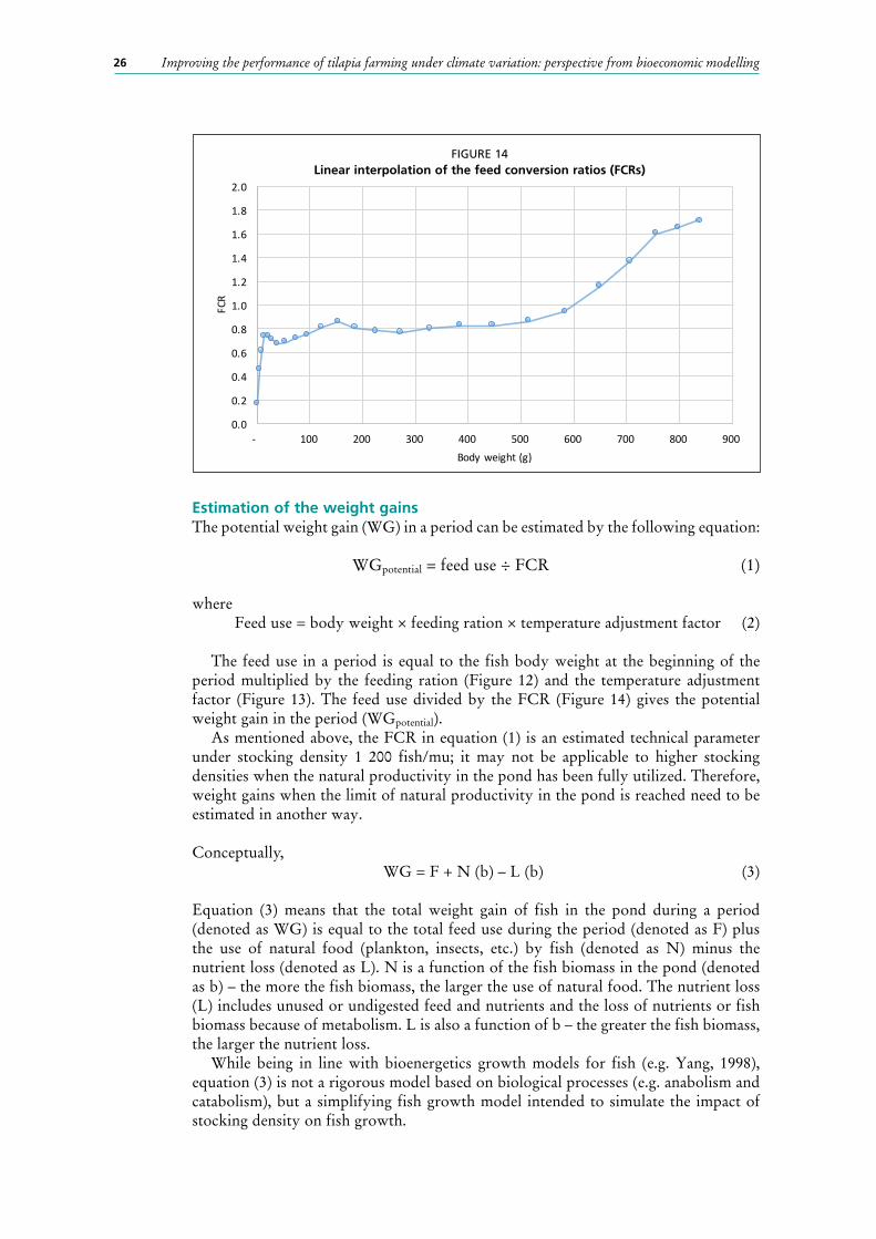
Improving the performance of tilapia farming under climate variation: perspective from bioeconomic modelling26
Estimation of the weight gainsThe potential weight gain (WG) in a period can be estimated by the following equation:
WGpotential = feed use ÷ FCR (1)
where Feed use = body weight × feeding ration × temperature adjustment factor (2)
The feed use in a period is equal to the fish body weight at the beginning of the period multiplied by the feeding ration (Figure 12) and the temperature adjustment factor (Figure 13). The feed use divided by the FCR (Figure 14) gives the potential weight gain in the period (WGpotential).
As mentioned above, the FCR in equation (1) is an estimated technical parameter under stocking density 1 200 fish/mu; it may not be applicable to higher stocking densities when the natural productivity in the pond has been fully utilized. Therefore, weight gains when the limit of natural productivity in the pond is reached need to be estimated in another way.
Conceptually, WG = F + N (b) – L (b) (3)
Equation (3) means that the total weight gain of fish in the pond during a period (denoted as WG) is equal to the total feed use during the period (denoted as F) plus the use of natural food (plankton, insects, etc.) by fish (denoted as N) minus the nutrient loss (denoted as L). N is a function of the fish biomass in the pond (denoted as b) – the more the fish biomass, the larger the use of natural food. The nutrient loss (L) includes unused or undigested feed and nutrients and the loss of nutrients or fish biomass because of metabolism. L is also a function of b – the greater the fish biomass, the larger the nutrient loss.
While being in line with bioenergetics growth models for fish (e.g. Yang, 1998), equation (3) is not a rigorous model based on biological processes (e.g. anabolism and catabolism), but a simplifying fish growth model intended to simulate the impact of stocking density on fish growth.
0.0
0.2
0.4
0.6
0.8
1.0
1.2
1.4
1.6
1.8
2.0
- 100 200 300 400 500 600 700 800 900
FCR
Bodyweight(g)
FIGURE 14Linear interpolation of the feed conversion ratios (FCRs)
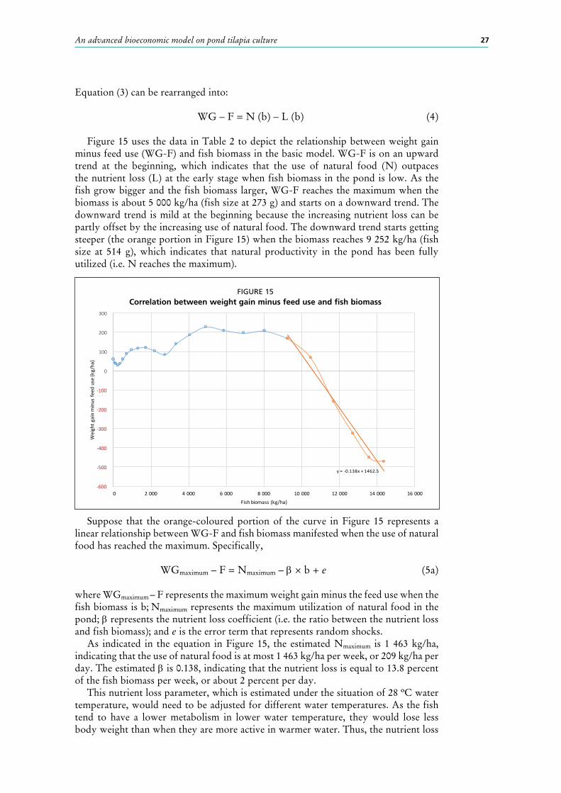
27An advanced bioeconomic model on pond tilapia culture
Equation (3) can be rearranged into:
WG – F = N (b) – L (b) (4)
Figure 15 uses the data in Table 2 to depict the relationship between weight gain minus feed use (WG-F) and fish biomass in the basic model. WG-F is on an upward trend at the beginning, which indicates that the use of natural food (N) outpaces the nutrient loss (L) at the early stage when fish biomass in the pond is low. As the fish grow bigger and the fish biomass larger, WG-F reaches the maximum when the biomass is about 5 000 kg/ha (fish size at 273 g) and starts on a downward trend. The downward trend is mild at the beginning because the increasing nutrient loss can be partly offset by the increasing use of natural food. The downward trend starts getting steeper (the orange portion in Figure 15) when the biomass reaches 9 252 kg/ha (fish size at 514 g), which indicates that natural productivity in the pond has been fully utilized (i.e. N reaches the maximum).
Suppose that the orange-coloured portion of the curve in Figure 15 represents a linear relationship between WG-F and fish biomass manifested when the use of natural food has reached the maximum. Specifically,
WGmaximum – F = Nmaximum – β × b + e (5a)
where WGmaximum – F represents the maximum weight gain minus the feed use when the fish biomass is b; Nmaximum represents the maximum utilization of natural food in the pond; β represents the nutrient loss coefficient (i.e. the ratio between the nutrient loss and fish biomass); and e is the error term that represents random shocks.
As indicated in the equation in Figure 15, the estimated Nmaximum is 1 463 kg/ha, indicating that the use of natural food is at most 1 463 kg/ha per week, or 209 kg/ha per day. The estimated β is 0.138, indicating that the nutrient loss is equal to 13.8 percent of the fish biomass per week, or about 2 percent per day.
This nutrient loss parameter, which is estimated under the situation of 28 ºC water temperature, would need to be adjusted for different water temperatures. As the fish tend to have a lower metabolism in lower water temperature, they would lose less body weight than when they are more active in warmer water. Thus, the nutrient loss
y= -0.138x+1462.5
-600
-500
-400
-300
-200
-100
0
100
200
300
0 2000 4000 6000 8000 10000 12000 14000 16000
Weightg
ainminusfe
eduse(kg/ha)
Fishbiomass(kg/ha)
FIGURE 15Correlation between weight gain minus feed use and fish biomass

Improving the performance of tilapia farming under climate variation: perspective from bioeconomic modelling28
parameter would tend to be lower in a lower water temperature. It is assumed that for water temperature below 30 ºC, the nutrient loss parameter would be adjusted by the adjustment factors described in Figure 13, whereas the nutrient loss adjustment factor would be 1.2 for a water temperature above 30 ºC.
In summary, the maximum weight gain during a period (a day or a week) is estimated by:
WGmaximum = F + Nmaximum – τ × β × b (5b)
where F is the feed use during the period; Nmaximum is the maximum natural productivity (1 463 kg/ha per week, or 209 kg/ha per day); τ × β is the temperature adjusted nutrient loss parameter (τ being the adjustment factor); and b is the fish biomass at the beginning of the period.
Finally, the fish weight gain during a period is determined by:
WG = min (WGpotential, WGmaximum) (6)
where WGpotential and WGmaximum are defined in equation (1) and (5b), respectively.
Equation (6) means that the weight gain is calculated by equation (1) and (2) when the result (i.e. the potential weight gain) is less or equal to the maximum weight gain estimated by equation (5b); otherwise, the weight gain is calculated by equation (5b).
Figure 16 shows the growth of fish body weight under different stocking densities with 1 g fingerlings and constant water temperature at 28 ºC. The results show that the advanced model captures the common pattern in fish outgrowing that a higher stocking density would tend to slow down the fish growth – while fish can grow to 838 g in 24 weeks under 1 200 fish/mu; it would only reach 616 g when the stocking density doubles to 2 400 fish/mu.
Carrying capacityThe original data used to calibrate the basic and advanced models (Tables 2 and 3) describe the fish growth pattern up to about 840 g. With the 1 200 fish/mu stocking
2400fish/mu,616g
1200fish/mu,834g
0
100
200
300
400
500
600
700
800
900
1 2 3 4 5 6 7 8 9 10 11 12 13 14 15 16 17 18 19 20 21 22 23 24 25
Fishbodyweight(g)
Growing period (weeks)1200fish/mu 1500fish/mu 1800fish/mu 2100fish/mu 2400fish/mu
FIGURE 16Fish growth path under different stocking densities
(1 g fingerlings and 28 °C water temperature)
29An advanced bioeconomic model on pond tilapia culture
density, this means that the fish biomass in the pond would be less than 16 000 kg/ha when the fish reach the maximum size.
It is therefore assumed that the carrying capacity in the advanced model is 16 000 kg/ha; the farmer would harvest the fish before the fish biomass in the pond reaches the capacity. Farming under the carrying capacity allows the farmer to avoid incurring additional costs (e.g. electricity cost for extra aeration, cost for fish health management and cost from fish mortality) that are not captured by the model.
Daily model weekly analysisAlthough the advanced model simulates the daily growth of fish, it would be overly cumbersome to conduct daily analysis, which entails the examination of over 360 possible stocking dates within a year. For simplicity, only 52 weekly stocking dates (i.e. 1 January, 8 January, 15 January, and so on) will be examined.
In order to facilitate the weekly analysis, a calendar year in the advanced model includes only 364 days (i.e. exactly 52 weeks) – there are 28 days in February and 30 days in December, whereas the number of days in other months are considered normal. The date at the end of each week is used to identify that week. For example, the week of 8 January represents the week from 2 January to 8 January.
SummaryTo summarize, in the advanced model the stocking timing, stocking density and initial fingerling size need to be determined first. Then the feed use and weight gain in the first day can be calculated by equation (2) and (6), respectively, and the body weight in the second day would be determined accordingly. The feed use and weight gain in the second day and body weight in the third day can be determined similarly, and so on. Finally, when the harvest date is determined, the harvest size and total feed use can be calculated, and so can other cost items similar to the basic model.
The advanced model captures the impacts of water temperature on feeding and hence fish growth, and accounts for the limit of natural productivity so that the stylized fact of higher stocking density slowing down fish growth is captured in the model.
The advanced model can be used to examine the impacts of various factors (including water temperature, stocking timing, stocking density, fingerling size and/or growing period) on farming performance and identify optimal farming arrangements.
Limited by data availability, the advanced model simulates the growth of GIFT tilapia under different situations based on the growth pattern of GIFT tilapia under a specific situation (1 g fingerlings stocked at 1 200 fish/mu density). The simulation can be improved by more data and understanding of the relationship between feed use and fish growth under different water temperature and/or stocking density.
3.2 IMPACTS OF STOCKING TIMING ON FARMING PERFORMANCEWith seasonal variation in the water temperature, the stocking timing matters for farming performance – a crop that is grown in more favourable water temperatures would tend to have better performance. The advanced model calibrated with seasonal variation in the water temperature is used to assess the profitability under different stocking timings.
Calibrating the seasonal water temperature variationThe daily temperature pattern in 2014 in Wenchang, Hainan province,13 is used to calibrate the water temperature in the advanced model. Based on Xu, Wang and Chen
13 Wenchang is a city in Hainan province in China. The temperature data have been obtained from the site http://tianqi.2345.com/wea_history/59856.htm (in Chinese).
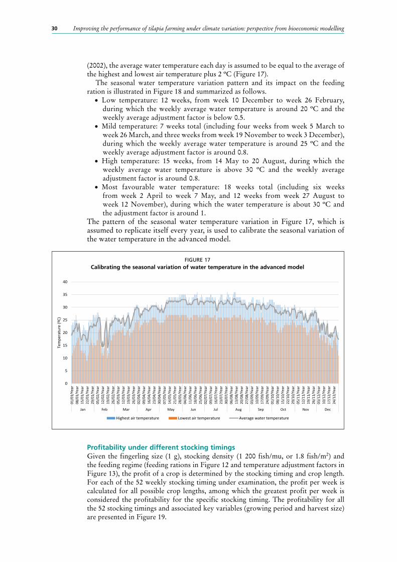
Improving the performance of tilapia farming under climate variation: perspective from bioeconomic modelling30
(2002), the average water temperature each day is assumed to be equal to the average of the highest and lowest air temperature plus 2 ºC (Figure 17).
The seasonal water temperature variation pattern and its impact on the feeding ration is illustrated in Figure 18 and summarized as follows.
• Low temperature: 12 weeks, from week 10 December to week 26 February, during which the weekly average water temperature is around 20 ºC and the weekly average adjustment factor is below 0.5.
• Mild temperature: 7 weeks total (including four weeks from week 5 March to week 26 March, and three weeks from week 19 November to week 3 December), during which the weekly average water temperature is around 25 ºC and the weekly average adjustment factor is around 0.8.
• High temperature: 15 weeks, from 14 May to 20 August, during which the weekly average water temperature is above 30 ºC and the weekly average adjustment factor is around 0.8.
• Most favourable water temperature: 18 weeks total (including six weeks from week 2 April to week 7 May, and 12 weeks from week 27 August to week 12 November), during which the water temperature is about 30 ºC and the adjustment factor is around 1.
The pattern of the seasonal water temperature variation in Figure 17, which is assumed to replicate itself every year, is used to calibrate the seasonal variation of the water temperature in the advanced model.
Profitability under different stocking timingsGiven the fingerling size (1 g), stocking density (1 200 fish/mu, or 1.8 fish/m2) and the feeding regime (feeding rations in Figure 12 and temperature adjustment factors in Figure 13), the profit of a crop is determined by the stocking timing and crop length. For each of the 52 weekly stocking timing under examination, the profit per week is calculated for all possible crop lengths, among which the greatest profit per week is considered the profitability for the specific stocking timing. The profitability for all the 52 stocking timings and associated key variables (growing period and harvest size) are presented in Figure 19.
0
5
10
15
20
25
30
35
40
01/0
1/Ye
ar08
/01/
Year
15/0
1/Ye
ar22
/01/
Year
29/0
1/Ye
ar05
/02/
Year
12/0
2/Ye
ar19
/02/
Year
26/0
2/Ye
ar05
/03/
Year
12/0
3/Ye
ar19
/03/
Year
26/0
3/Ye
ar02
/04/
Year
09/0
4/Ye
ar16
/04/
Year
23/0
4/Ye
ar30
/04/
Year
07/0
5/Ye
ar14
/05/
Year
21/0
5/Ye
ar28
/05/
Year
04/0
6/Ye
ar11
/06/
Year
18/0
6/Ye
ar25
/06/
Year
02/0
7/Ye
ar09
/07/
Year
16/0
7/Ye
ar23
/07/
Year
30/0
7/Ye
ar06
/08/
Year
13/0
8/Ye
ar20
/08/
Year
27/0
8/Ye
ar03
/09/
Year
10/0
9/Ye
ar17
/09/
Year
24/0
9/Ye
ar01
/10/
Year
08/1
0/Ye
ar15
/10/
Year
22/1
0/Ye
ar29
/10/
Year
05/1
1/Ye
ar12
/11/
Year
19/1
1/Ye
ar26
/11/
Year
03/1
2/Ye
ar10
/12/
Year
17/1
2/Ye
ar24
/12/
Year
Jan Feb Mar Apr May Jun Jul Aug Sep Oct Nov Dec
Tem
pera
ture
(ºC)
Highest air temperature Lowest air temperature Average water temperature
FIGURE 17Calibrating the seasonal variation of water temperature in the advanced model

31An advanced bioeconomic model on pond tilapia culture
December to February (26 November to 26 February)When stocking the fish on 26 November (1 g fingerlings, 1 200 fish/mu), the maximum achievable profit would be CNY 892/ha per week when harvesting 612 g fish after 28 weeks on 11 June the next year. This is the lowest profitability among all 52 stocking timings (Figure 19).
The low profitability is due to slow growth at the fingerling stage in winter – it would take 17 weeks from 26 November to 26 March the next year for the fish to reach 105 g, whereas it would take only 11 weeks in the warmer water from 26 March to 11 June for the fish to reach 612 g (Figure 20).
19.7
21.7
19.9
18.3
21.4
23.2
21.1
18.8
22.0
25.1 24.8 24.924.4
29.3
27.4
29.030.1 29.9
28.7
31.532.4 32.4
32.9
31.632.1 32.3 31.9 32.4 32.0
30.831.6 32.0
32.632.1
30.8 30.5 30.4 30.5 30.1 30.4
29.1
27.728.3 28.1 27.9 27.9
25.4
26.7 26.6
22.3
20.7
19.3
0.28
0.44
0.27
0.18
0.40
0.55
0.44
0.27
0.47
0.80 0.75 0.75
0.69
1.13
0.97
1.10 1.13 1.12
1.07
0.89
0.75 0.75
0.66
0.90
0.81 0.77
0.82
0.75 0.81
0.94 0.89
0.81
0.72
0.80
1.02 1.07
1.03 1.06 1.08 1.09 1.09
0.98 1.03 1.02 1.01 1.00
0.82
0.91 0.89
0.48
0.37
0.28
01-Ja
n
08-Ja
n
15-Ja
n
22-Ja
n
29-Ja
n
05-F
eb
12-F
eb
19-F
eb
26-F
eb
05-M
ar
12-M
ar
19-M
ar
26-M
ar
02-A
pr
09-A
pr
16-A
pr
23-A
pr
30-A
pr
07-M
ay
14-M
ay
21-M
ay
28-M
ay
04-Ju
n
11-Ju
n
18-Ju
n
25-Ju
n
02-Ju
l
09-Ju
l
16-Ju
l
23-Ju
l
30-Ju
l
06-A
ug
13-A
ug
20-A
ug
27-A
ug
03-S
ep
10-S
ep
17-S
ep
24-S
ep
01-O
ct
08-O
ct
15-O
ct
22-O
ct
29-O
ct
05-N
ov
12-N
ov
19-N
ov
26-N
ov
03-D
ec
10-D
ec
17-D
ec
24-D
ec
Jan Feb Mar Apr May Jun Jul Aug Sep Oct Nov Dec
Weekly average water temperature (ºC) Temperature adjustment factor for feed ration
FIGURE 18Average weekly water temperature and corresponding temperature adjustment factors
597530
704 680
522
664612
1424 14301465
1921
1560
1059
892
2119
23
2018
28 28
-
5
10
15
20
25
30
35
40
45
50
0
200
400
600
800
1000
1200
1400
1600
1800
2000
01/01/1s
tyear
08/01/1s
tyear
15/01/1s
tyear
22/01/1s
tyear
29/01/1s
tyear
05/02/1s
tyear
12/02/1s
tyear
19/02/1s
tyear
26/02/1s
tyear
05/03/1s
tyear
12/03/1s
tyear
19/03/1s
tyear
26/03/1s
tyear
02/04/1s
tyear
09/04/1s
tyear
16/04/1s
tyear
23/04/1s
tyear
30/04/1s
tyear
07/05/1s
tyear
14/05/1s
tyear
21/05/1s
tyear
28/05/1s
tyear
04/06/1s
tyear
11/06/1s
tyear
18/06/1s
tyear
25/06/1s
tyear
02/07/1s
tyear
09/07/1s
tyear
16/07/1s
tyear
23/07/1s
tyear
30/07/1s
tyear
06/08/1s
tyear
13/08/1s
tyear
20/08/1s
tyear
27/08/1s
tyear
03/09/1s
tyear
10/09/1s
tyear
17/09/1s
tyear
24/09/1s
tyear
01/10/1s
tyear
08/10/1s
tyear
15/10/1s
tyear
22/10/1s
tyear
29/10/1s
tyear
05/11/1s
tyear
12/11/1s
tyear
19/11/1s
tyear
26/11/1s
tyear
03/12/1s
tyear
10/12/1s
tyear
17/12/1s
tyear
24/12/1s
tyear
Jan Feb Mar Apr May Jun Jul Aug Sep Oct Nov Dec
Waterte
mpe
rature(ºC)o
rgrowingpe
riod(w
eeks)
Maxim
umprofit(CN
Y/ha
/wee
k)orh
arve
stsize(g
)
Stockingtiming
Average weekly water temperature (ºC) Optimalharvest size(g) Maximumprofit(CNY/ha/week) Optimalgrowingperiod (weeks)
FIGURE 19Profitability of individual crops under different stocking timings

Improving the performance of tilapia farming under climate variation: perspective from bioeconomic modelling32
Moving the stocking timing from 26 November forward would increase the profitability by reducing the time in the low temperature, less productive season and increasing the time in the more productive season; the upward trend would continue until 26 February (Figure 19).
March and April (26 February to 30 April)The profitability of stocking the fish on 26 February would be CNY 1 424/ha per week, achieved when harvesting 597 g fish after 21 weeks on 23 July (Figure 20). Postponing the stocking timing a little within March would not affect the profitability much, but the optimal growing period tends to be shortened; hence, the optimal harvest size is reduced in order to avoid the inefficiency of growing large fish in the hot summer (Figure 19). For example, when stocking the fish on 26 March, the maximum achievable profitability would be CNY 1 430/ha per week when harvesting 530 g fish after 19 weeks on 6 August (Figure 20).
Moving the stocking timing from the end of March towards the end of April would slightly increase the profitability (Figure 19). The profitability of stocking on 30 April would be CNY 1 465/ha per week, achieved when harvesting 704 g fish after 23 weeks on 1 October. The optimal growing period is four weeks longer than stocking on 26 March because the cooler weather in September is more suitable for growing large fish.
May to mid-July (30 April to 16 July)Moving the stocking timing from the end of April towards mid-July would significantly increase profitability (Figure 19) because of reducing the exposure to a high temperature, relatively less conducive season from May to August and increasing exposure to a more conducive season in September and October. The optimal growing period is declining so as to reduce the exposure to the low temperature, less conducive season in December. Accordingly, the optimal harvest size is declining.
Stocking the fish on 16 July would be the most profitable among the 52 weekly stocking timings; the maximum profit is CNY 1 921/ha per week, achieved when harvesting 680 g fish after 20 weeks in early December before the low temperature season starts (Figure 20).
20weeks,1921CNY/ha/week, 680g
28weeks,892CNY/ha/week,612g21weeks,1424CNY/ha/week, 597g
23weeks,1465CNY/ha/week, 704g
19weeks,1430CNY/ha/week, 530g
18weeks,1560CNY/ha/week, 522g
28weeks,1193CNY/ha/week, 688g
0
5
10
15
20
25
30
35
40
45
50
0
100
200
300
400
500
600
700
800
900
1000
01/01/1styear
15/01/1styear
29/01/1styear
12/02/1styear
26/02/1styear
12/03/1styear
26/03/1styear
09/04/1styear
23/04/1styear
07/05/1styear
21/05/1styear
04/06/1styear
18/06/1styear
02/07/1styear
16/07/1styear
30/07/1styear
13/08/1styear
27/08/1styear
10/09/1styear
24/09/1styear
08/10/1styear
22/10/1styear
05/11/1styear
19/11/1styear
03/12/1styear
17/12/1styear
01/01/2ndyear
15/01/2ndyear
29/01/2ndyear
12/02/2ndyear
26/02/2ndyear
12/03/2ndyear
26/03/2ndyear
09/04/2ndyear
23/04/2ndyear
07/05/2ndyear
21/05/2ndyear
04/06/2ndyear
18/06/2ndyear
02/07/2ndyear
16/07/2ndyear
30/07/2ndyear
13/08/2ndyear
27/08/2ndyear
10/09/2ndyear
24/09/2ndyear
08/10/2ndyear
22/10/2ndyear
05/11/2ndyear
19/11/2ndyear
03/12/2ndyear
17/12/2ndyear
Jan Feb Mar Apr May Jun Jul Aug Sep Oct Nov Dec Jan Feb Mar Apr May Jun Jul Aug Sep Oct Nov Dec
Watertemperature(ºC)
Size(g)
Stockingtiming
Averageweeklywatertemperature (ºC)
FIGURE 20Growth patterns and farming performance of individual crops under different stocking timings
(1 g fingerlings, 1 200 fish/mu)

33An advanced bioeconomic model on pond tilapia culture
Mid-July to August (16 July to 27 August)Moving the stocking timing from mid-July towards the end of August would reduce the profitability because the farmer would need to shorten the optimal growing period in order to reduce the exposure to the low temperature season in December (Figure 19). For example, the profitability of stocking on 13 August would be CNY 1 560/ha per week, achieved when harvesting 522 g fish after 18 weeks on 17 December (Figure 20).
September to November (27 August to 26 November)Starting during late August, the growing cycle has to enter the low temperature season from December on in order to reach a desirable size (over 500 g). Moving the stocking timing forward during the period from September to November would increase the exposure to the low temperature season and hence reduce profitability. The growing period would be much longer than stocking from February to August, whereas the optimal harvest size would not differ much (Figure 19).
For example, the profitability of stocking on 8 October would be CNY 1 059/ha per week, achieved when harvesting 664 g fish in 28 weeks on 23 April. This cycle also covers the entire winter, but its profitability is higher than the one with the lowest profitability (i.e. stocking on 26 November) because the fish enter the low temperature season with a relatively large size – in this situation, the fish would reach about 70 g on 26 November (seven weeks after stocking).
SummaryIn summary, stocking 1 g fingerlings (1 200 fish/mu) in the summer on 16 July would be the most profitable; CNY 1 921/ha per week maximum profitability (20-week growing period, 680 g harvest size) is more than double the minimum profitability (CNY 892/ha per week, 28-week growing period, 612 g harvest size) when stocking at the beginning of the low temperature season on 26 November.
3.3 IMPACTS OF STOCKING DENSITY ON FARMING PERFORMANCEGenerally speaking, fish growth tends to slow down under higher stocking density because there would be more fish competing for food, oxygen and space. This stylized fact is captured in the advanced model (Figure 16).
Given the 1 g fingerling size and the feeding regime, the fish growth pattern under different stocking density from 1 200 fish/mu to 2 400 fish/mu is simulated and their profitability examined. The results indicate that, generally speaking, increasing the stocking density from 1 200 fish/mu onwards would tend to push the optimal stocking timing from 16 July forward,14 shorten the optimal growing period and reduce the optimal harvest size, and profitability would increase until the density reaches around 2 000 fish/mu and then decline (Table 7).
Increasing the stocking density from 1 200 fish/mu to 1 300 fish/mu or 1 400 fish/mu would not change the optimal stocking timing or growing period. Although the harvest size would decrease slightly, the fish biomass would increase because more fish would be harvested under the higher density. The profitability would be higher accordingly. Under the 1 200 fish/mu stocking density, the farmer can grow the fish longer than 20 weeks for higher fish biomass at harvest, but doing so would reduce the profit because of the inefficiency (i.e. higher FCR) in farming large fish.
The profitability of stocking 1 500 fish/mu on 16 July would be CNY 2 338/ha per week (Figure 21), higher than the profitability under 1 200, 1 300 or 1 400 fish/mu (Table 7). However, the stocking timing of 16 July is not optimal for 1 500 fish/mu – postponing the stocking timing by one week on 23 July, yet harvesting at the same
14 One exception is for the stocking density 2 100 fish/mu, under which the optimal stocking timing is 2 July so that the harvest size can be greater than 500 g for the higher price.

Improving the performance of tilapia farming under climate variation: perspective from bioeconomic modelling34
time (i.e. reducing the growing period by one week) would increase profitability to CNY 2 365/ha per week, even though the one-week delay in stocking and the one-week decrease in the growing period would reduce the harvest size from 646 g to 604 g, and productivity from 661 kg/ha per week to 647 kg/ha per week (Figure 21). This is another example showing that technical and economic performance may not be consistent.
From 1 500 fish/mu to 2 000 fish/mu, the optimal growing period is the same at 19 weeks, whereas the stocking timing could be slightly different. The increased
32 32 32 31 32 32 33 32 31 31 30 31 30 30 29 28 28 28 28 2825 27 27
22 21 19 2022 20 18
21 2321
1922
25 25 25 24
16-July,1200fish/mu,20weeks1921CNY/ha/week,680g
556kg/ha/week
16-July,1500fish/mu,20weeks2338CNY/ha/week,646g
661kg/ha/week
23-July,1500fish/mu,19weeks2365CNY/ha/week,604g
647kg/ha/week
0
100
200
300
400
500
600
700
800
900
02/07/1styear
09/07/1styear
16/07/1styear
23/07/1styear
30/07/1styear
06/08/1styear
13/08/1styear
20/08/1styear
27/08/1styear
03/09/1styear
10/09/1styear
17/09/1styear
24/09/1styear
01/10/1styear
08/10/1styear
15/10/1styear
22/10/1styear
29/10/1styear
05/11/1styear
12/11/1styear
19/11/1styear
26/11/1styear
03/12/1styear
10/12/1styear
17/12/1styear
24/12/1styear
01/01/2ndyear
08/01/2ndyear
15/01/2ndyear
22/01/2ndyear
29/01/2ndyear
05/02/2ndyear
12/02/2ndyear
19/02/2ndyear
26/02/2ndyear
05/03/2ndyear
12/03/2ndyear
19/03/2ndyear
26/03/2ndyear
Jul Aug Sep Oct Nov Dec Jan Feb Mar
Size(g)
Stockingtiming
Averageweeklywatertemperature (ºC)
FIGURE 21Growth patterns and farming performance of individual crops
under different stocking density (1 g fingerlings)
TABLE 7Optimal farming arrangements and performance under different stocking density
Stocking density(fish/mu)
Optimal farming arrangement
Stocking timingGrowing period
(weeks)
Harvest size(g)
Fish biomass at harvest
(kg/ha)
Productivity(kg/ha/week)
Profitability(CNY/ha/week)
1 200 16/07/1st year 20 680 12 234 556 1 921
1 300 16/07/1st year 20 673 13 121 596 2 105
1 400 16/07/1st year 20 661 13 875 631 2 239
1 500 23/07/1st year 19 604 13 591 647 2 365
1 600 30/07/1st year 19 580 13 925 663 2 471
1 700 30/07/1st year 19 572 14 577 694 2 595
1 800 30/07/1st year 19 561 15 144 721 2 687
1 900 06/08/1st year 19 540 15 388 733 2 797
2 000 06/08/1st year 19 531 15 929 759 2 887
2 100 02/07/1st year 19 505 15 902 757 2 470
2 200 20/08/1st year 17 446 14 721 775 1 588
2 300 20/08/1st year 17 441 15 216 801 1 644
2 400 20/08/1st year 17 436 15 682 825 1 677
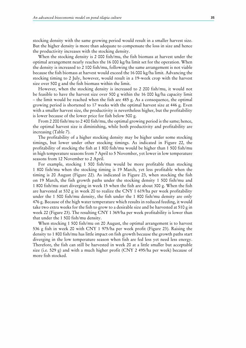
35An advanced bioeconomic model on pond tilapia culture
stocking density with the same growing period would result in a smaller harvest size. But the higher density is more than adequate to compensate the loss in size and hence the productivity increases with the stocking density.
When the stocking density is 2 000 fish/mu, the fish biomass at harvest under the optimal arrangement nearly reaches the 16 000 kg/ha limit set for the operation. When the density is increased to 2 100 fish/mu, following the same arrangement is not viable because the fish biomass at harvest would exceed the 16 000 kg/ha limit. Advancing the stocking timing to 2 July, however, would result in a 19-week crop with the harvest size over 500 g and the fish biomass within the limit.
However, when the stocking density is increased to 2 200 fish/mu, it would not be feasible to have the harvest size over 500 g within the 16 000 kg/ha capacity limit – the limit would be reached when the fish are 485 g. As a consequence, the optimal growing period is shortened to 17 weeks with the optimal harvest size at 446 g. Even with a smaller harvest size, the productivity is nevertheless higher, but the profitability is lower because of the lower price for fish below 500 g.
From 2 200 fish/mu to 2 400 fish/mu, the optimal growing period is the same; hence, the optimal harvest size is diminishing, while both productivity and profitability are increasing (Table 7).
The profitability of a higher stocking density may be higher under some stocking timings, but lower under other stocking timings. As indicated in Figure 22, the profitability of stocking the fish at 1 800 fish/mu would be higher than 1 500 fish/mu in high temperature seasons from 7 April to 5 November, yet lower in low temperature seasons from 12 November to 2 April.
For example, stocking 1 500 fish/mu would be more profitable than stocking 1 800 fish/mu when the stocking timing is 19 March, yet less profitable when the timing is 20 August (Figure 22). As indicated in Figure 23, when stocking the fish on 19 March, the fish growth paths under the stocking density 1 500 fish/mu and 1 800 fish/mu start diverging in week 15 when the fish are about 300 g. When the fish are harvested at 532 g in week 20 to realize the CNY 1 619/ha per week profitability under the 1 500 fish/mu density, the fish under the 1 800 fish/mu density are only 476 g. Because of the high water temperature which results in reduced feeding, it would take two extra weeks for the fish to grow to a desirable size and be harvested at 510 g in week 22 (Figure 23). The resulting CNY 1 369/ha per week profitability is lower than that under the 1 500 fish/mu density.
When stocking 1 500 fish/mu on 20 August, the optimal arrangement is to harvest 536 g fish in week 20 with CNY 1 975/ha per week profit (Figure 23). Raising the density to 1 800 fish/mu has little impact on fish growth because the growth paths start diverging in the low temperature season when fish are fed less yet need less energy. Therefore, the fish can still be harvested in week 20 at a little smaller but acceptable size (i.e. 529 g) and with a much higher profit (CNY 2 495/ha per week) because of more fish stocked.
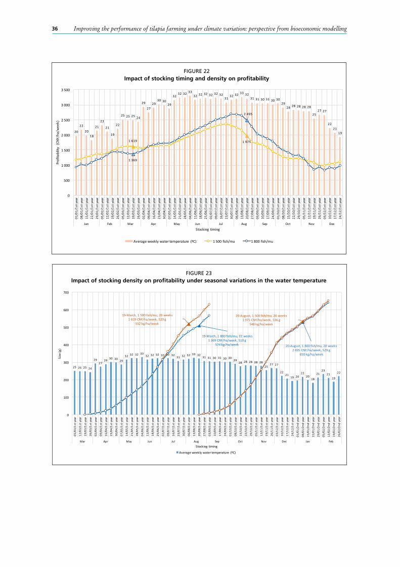
Improving the performance of tilapia farming under climate variation: perspective from bioeconomic modelling36
25 25 25 24
2927
29 30 30 2932 32 32 33
32 32 32 32 32 3231 32 32 33 32
31 31 30 31 30 3029
28 28 28 28 2825
27 27
2221
19 2022
2018
2123
2119
22
19-March,1500fish/mu,20weeks1619CNY/ha/week,520g
532kg/ha/week
19-March,1800fish/mu,22weeks1369CNY/ha/week,510g
574kg/ha/week 20-August,1800fish/mu,20weeks2495CNY/ha/week,529g
650kg/ha/week
20-August,1500fish/mu,20weeks1975CNY/ha/week,536g
548kg/ha/week
0
100
200
300
400
500
600
700
05/03/1styear
12/03/1styear
19/03/1styear
26/03/1styear
02/04/1styear
09/04/1styear
16/04/1styear
23/04/1styear
30/04/1styear
07/05/1styear
14/05/1styear
21/05/1styear
28/05/1styear
04/06/1styear
11/06/1styear
18/06/1styear
25/06/1styear
02/07/1styear
09/07/1styear
16/07/1styear
23/07/1styear
30/07/1styear
06/08/1styear
13/08/1styear
20/08/1styear
27/08/1styear
03/09/1styear
10/09/1styear
17/09/1styear
24/09/1styear
01/10/1styear
08/10/1styear
15/10/1styear
22/10/1styear
29/10/1styear
05/11/1styear
12/11/1styear
19/11/1styear
26/11/1styear
03/12/1styear
10/12/1styear
17/12/1styear
24/12/1styear
01/01/2ndyear
08/01/2ndyear
15/01/2ndyear
22/01/2ndyear
29/01/2ndyear
05/02/2ndyear
12/02/2ndyear
19/02/2ndyear
26/02/2ndyear
Mar Apr May Jun Jul Aug Sep Oct Nov Dec Jan Feb
Size(g)
Stockingtiming
Averageweeklywatertemperature (ºC)
FIGURE 23Impact of stocking density on profitability under seasonal variations in the water temperature
20
2220
18
2123
21
19
22
25 25 25 24
2927
2930 30
29
3232 32 33
32 32 32 3232 32
3132 32
33 3231 31 30 31 30 30
2928 28 28 28 28
2527 27
2221
19
1619 1975
1369
2495
0
500
1000
1500
2000
2500
3000
3500
01/01/1styear
08/01/1styear
15/01/1styear
22/01/1styear
29/01/1styear
05/02/1styear
12/02/1styear
19/02/1styear
26/02/1styear
05/03/1styear
12/03/1styear
19/03/1styear
26/03/1styear
02/04/1styear
09/04/1styear
16/04/1styear
23/04/1styear
30/04/1styear
07/05/1styear
14/05/1styear
21/05/1styear
28/05/1styear
04/06/1styear
11/06/1styear
18/06/1styear
25/06/1styear
02/07/1styear
09/07/1styear
16/07/1styear
23/07/1styear
30/07/1styear
06/08/1styear
13/08/1styear
20/08/1styear
27/08/1styear
03/09/1styear
10/09/1styear
17/09/1styear
24/09/1styear
01/10/1styear
08/10/1styear
15/10/1styear
22/10/1styear
29/10/1styear
05/11/1styear
12/11/1styear
19/11/1styear
26/11/1styear
03/12/1styear
10/12/1styear
17/12/1styear
24/12/1styear
Jan Feb Mar Apr May Jun Jul Aug Sep Oct Nov Dec
Profitability(CNY/ha/week)
Stockingtiming
Averageweeklywatertemperature (ºC) 1500fish/mu 1800fish/mu
FIGURE 22Impact of stocking timing and density on profitability

37
4. Optimizing crop arrangements for better performance
The examination of the impacts of farming arrangements on the profitability of an individual crop in the previous section provides useful guidance for farmers to improve their farming performance. However, an arrangement that maximizes the profitability of an individual crop may not be optimal for the overall profitability of a multiple-crop production cycle.
In this section, the advanced model is used to simulate the performance of various crop arrangements and identify the crop arrangement that maximizes the overall profitability of a production cycle. As seasonal water temperature variation tends to repeat over years, the duration of a production cycle repeatable over years should be equal to an integer number of years (e.g. 1 year, 2 years, 3 years, and so on). A production cycle could be 1 year 1 crop, 1 year 2 crops, 1 year 3 crops, 2 year 2 crops, 2 year 3 crops, 2 year 4 crops, 2 year 5 crops, and so on. The overall profitability of a production cycle is gauged by the sum of the profits of all crops in the cycle divided by the duration of the cycle and can be measured by profit per hectare per week or by profit per hectare per year.
In the advanced model, crop arrangements for a production cycle include the selection of four key variables (stocking timing, fingerling size, stocking density and growing period) for each crop in the cycle. Given the feeding regime built in the model, the harvest size is endogenously determined when the four variables are selected.
Although daily fish growth is simulated in the model, the analysis is conducted weekly. Therefore, only 52 weekly stocking timings are considered. For simplicity, only 1 g fingerlings are considered in most simulations except for the examination of a two-tier farming system where the farmer can select four fingerling sizes (1 g, 50 g, 100 g and 150 g) for stocking in outgrowing ponds. The range of stocking density varies in different simulations. For example, for arrangements with 1 g fingerlings and over 500 g harvest size, 17 stocking densities from 800 fish/mu to 2 400 fish/mu with a 100 fish/mu increment (i.e. 800 fish/mu, 900 fish/mu, 1 000 fish/mu, and so on) are considered,15 whereas for arrangements intended for the production of large fingerlings, the range of stocking density is set at 1 500–110 000 fish/mu with a 500 fish/mu increment. In total, 28 growing periods from 3 weeks to 30 weeks are considered because there is no relevant crop arrangement outside this growing period range that would result in a positive profit or fish biomass within the 16 000 kg/ha limit.
The combination of the four key variables within their ranges would result in a number of relevant single-crop arrangements. These single-crop arrangements are used as “building blocks” to simulate all cases of a multiple-crop production cycle (e.g. 1 year 2 crops, 2 year 5 crops,16 or 1 year 3 crops) from which profit maximizing arrangements can be identified.
15 The upper bound is set at 2 400 fish/mu because there is no crop arrangement for density equal to or higher than 2 500 fish/mu that would result in a positive profit. The 800 fish/mu lower bound is selected because crop arrangements with stocking density lower than 800 fish/mu tend to be less profitable; and farmers in reality usually do not stock the fish below it.
16 There are too many possible cases for 2 years 5 crops to be simulated comprehensively. Thus, only part of the possible cases are examined.

Improving the performance of tilapia farming under climate variation: perspective from bioeconomic modelling38
4.1 PROFIT MAXIMIZATION FOR INDIVIDUAL CROPS ≠ OVERALL PROFIT MAXIMIZATION In the basic model where the water temperature is constant, the profit maximizing arrangement for a single crop can be repeated over time. However, in the advanced model, which captures seasonal variation in the water temperature, farmers would need to maximize the overall profitability of multiple crops that are usually subject to different water temperature patterns.
A stepwise strategy is to first determine the profit maximizing arrangement for the first crop, then determine the one for the second crop, the third crop, and so on. This seemingly straightforward strategy may nevertheless not maximize the overall profitability.
For example, when stocking 1 g fingerlings at 1 200 fish/mu on 28 May, the most profitable arrangement is to harvest after 22 weeks on 29 October, with CNY 1 716/ha per week of profit. After two weeks for pond preparation, another crop should start on 11 November with the same stocking density. The most profitable arrangement for the second crop is to harvest after 26 weeks, on 14 May of the next year, with CNY 939/ha per week of profit. The two crops plus the time for pond preparation (two weeks for each crop) would take 52 weeks, which means that they constitute a 1-year-2-crop production cycle repeatable over years. As the maximum profitability is achieved in both crops, one may expect that their overall profit (CNY 1 297/ha per week) would be the maximum profitability for 1 year 2 crops starting on 28 May. This is, however, not the case.
If the farmer harvests the fish one week earlier on 22 October, the 21-week first crop would yield CNY 1 709/ha per week of profit, a little less than the maximum profitability (CNY 1 716/ha per week) achieved under the 22-week arrangement. However, shortening the first crop by one week allows the second crop to start one week earlier on 4 November and last one week longer (i.e. 27 weeks) when harvesting on 14 May the next year. The resulting profitability in the second crop of CNY 996/ha per week is about CNY 57/ha per week higher than the CNY 939/ha per week achieved under the 26-week second crop starting on 11 November. As the profitability gain from the second crop (57 CNY/ha/week) outweighs the profitability loss from the first crop (7 CNY/ha/week), the overall profitability of these two crops (CNY 1 311/ha per week) is greater than the CNY 1 297/ha per week profitability under the arrangement of stepwise profit maximization in both crops.
In the example above, the arrangement that maximizes the profitability of the first crop would result in a less opportune stocking timing for the second crop. Even with the maximum profitability achieved in both crops, the overall profitability is suboptimal, which can be improved by shortening the growing period of the first crop by one week.
In summary, as the harvest timing of a crop affects the stocking timing of the next one, the arrangement of an individual crop would affect not only its own performance but also that of the next crop. With such path dependency, the stepwise strategy that maximizes the profitability of individual crops separately is not necessarily a strategy that maximizes the overall profitability; farmers should take a holistic approach to maximize the overall profitability of multiple crops.
4.2 BENCHMARK ARRANGEMENT: 1 YEAR 2 CROPSFarmers normally have control over stocking timing, stocking density and crop length. They may not have access, however, to large-size fingerlings when there are no readily accessible commercial nurseries around, and they also lack technology, facilities or manpower to have on-farm nursing operations. Therefore, the situation where the farmer can only stock 1 g fingerlings will be considered first. This assumption would be relaxed later.

39Optimizing crop arrangements for better performance
Five arrangements – 1 year 1 crop, 1 year 2 crops, 1 year 3 crops, 2 years 3 crops, and 2 years 5 crops – are simulated. The results indicate that, given 1 g fingerlings, 1 year 2 crops is more profitable than other arrangements.
Given the water temperature pattern, the suitable growing period is from 15 to 30 weeks, depending on the stocking timing. Therefore, 1 year 1 crop or 2 years 3 crops (average 1 year 1.5 crops), under which the average growing period exceeds 30 weeks, would have to include a crop with an inefficiently long duration. On the other hand, 1 year 3 crops, under which the average growing period is about 15 weeks,17 would not be able to have a long enough growing period for all the three crops to be profitable – while a 15-week crop could be profitable under the most favourable water temperature, the growing period needs to be longer in the low-temperature season for the fish to reach desirable size. The arrangement of 2 years 5 crops (average 1 year 2.5 crops) is possible, but its overall profitability is generally lower than 1 year 2 crops.
Table 8 presents the profit maximizing arrangements under 1 year 2 crops for each of the 52 initial weekly stocking timings. The results are illustrated in Figure 24 and summarized below.
Symmetric arrangementsStocking on 27 August for the first crop and on 19 February the next year for the second crop would generate a total profit of CNY 90 352/ha per year, which is the maximum profitability for 1 year 2 crops starting on 27 August. Symmetrically, one may expect that stocking the first crop on 19 February and the second crop on 27 August would also be the profit-maximizing arrangement for 1 year 2 crops starting on 19 February. This is nevertheless not the case. For a 1-year-2-crop cycle starting on 19 February, the profit-maximizing arrangement would be to stock the first crop on 19 February and the second crop on 20 August, which would yield CNY 91 172/ha per year (Table 8).
However, among the 52 weekly stocking timings, there are 28 stocking timings (i.e. 14 pairs) with symmetric arrangements that are both profit maximizing. They
17 Excluding six weeks for pond preparation (two weeks for each crop), there are 46 weeks in total for three crops, which means the average crop length is about 15 weeks.
92491
78137
92491
06/08/1s
tyear
06/08/1s
tyear
06/08/1s
tyear
06/08/1s
tyear
20/08/1s
tyear
20/08/1s
tyear
20/08/1s
tyear
20/08/1s
tyear
27/08/1s
tyear
20/08/1s
tyear
03/09/1s
tyear
10/09/1s
tyear
17/09/1s
tyear
17/09/1s
tyear
24/09/1s
tyear
01/10/1s
tyear
01/10/1s
tyear
08/10/1s
tyear
15/10/1s
tyear
22/10/1s
tyear
29/10/1s
tyear
05/11/1s
tyear
12/11/1s
tyear
19/11/1s
tyear
19/11/1s
tyear
10/12/1s
tyear
17/12/1s
tyear
24/12/1s
tyear
08/01/2n
dyear
22/01/2n
dyear
22/01/2n
dyear
22/01/2n
dyear
05/03/2n
dyear
19/02/2n
dyear
19/02/2n
dyear
12/03/2n
dyear
19/03/2n
dyear
02/04/2n
dyear
09/04/2n
dyear
16/04/2n
dyear
30/04/2n
dyear
07/05/2n
dyear
14/05/2n
dyear
21/05/2n
dyear
28/05/2n
dyear
04/06/2n
dyear
11/06/2n
dyear
25/06/2n
dyear
09/07/2n
dyear
16/07/2n
dyear
09/07/2n
dyear
30/07/2n
dyear
Aug Sep Oct Nov Dec Jan Mar Feb Mar Apr May Jun Jul
-
10
20
30
40
50
60
70000
75000
80000
85000
90000
95000
100000
01/01/1s
tyear
08/01/1s
tyear
15/01/1s
tyear
22/01/1s
tyear
29/01/1s
tyear
05/02/1s
tyear
12/02/1s
tyear
19/02/1s
tyear
26/02/1s
tyear
05/03/1s
tyear
12/03/1s
tyear
19/03/1s
tyear
26/03/1s
tyear
02/04/1s
tyear
09/04/1s
tyear
16/04/1s
tyear
23/04/1s
tyear
30/04/1s
tyear
07/05/1s
tyear
14/05/1s
tyear
21/05/1s
tyear
28/05/1s
tyear
04/06/1s
tyear
11/06/1s
tyear
18/06/1s
tyear
25/06/1s
tyear
02/07/1s
tyear
09/07/1s
tyear
16/07/1s
tyear
23/07/1s
tyear
30/07/1s
tyear
06/08/1s
tyear
13/08/1s
tyear
20/08/1s
tyear
27/08/1s
tyear
03/09/1s
tyear
10/09/1s
tyear
17/09/1s
tyear
24/09/1s
tyear
01/10/1s
tyear
08/10/1s
tyear
15/10/1s
tyear
22/10/1s
tyear
29/10/1s
tyear
05/11/1s
tyear
12/11/1s
tyear
19/11/1s
tyear
26/11/1s
tyear
03/12/1s
tyear
10/12/1s
tyear
17/12/1s
tyear
24/12/1s
tyear
Jan Feb Mar Apr May Jun Jul Aug Sep Oct Nov Dec
2ndcrop
Averag
ewee
klywaterte
mpe
rature(ºC)
Totalp
rofit(CN
Y/ha
/yea
r)
1stcrop
Averageweeklywatertemperature (ºC) Totalprofit (CNY/ha/year)Stockingtiming
FIGURE 24Overall profitability under 1 year 2 crops (1 g fingerlings)
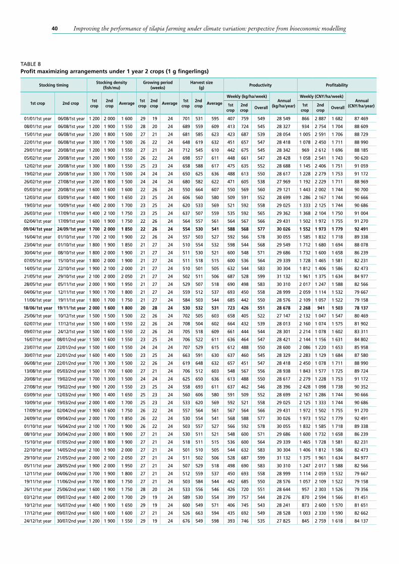
Improving the performance of tilapia farming under climate variation: perspective from bioeconomic modelling40
TABLE 8Profit maximizing arrangements under 1 year 2 crops (1 g fingerlings)
Stocking timingStocking density
(fish/mu)Growing period
(weeks)Harvest size
(g)Productivity Profitability
1st crop 2nd crop1st
crop2nd crop
Average1st
crop2nd crop
Average1st
crop2nd crop
Average
Weekly (kg/ha/week) Annual
(kg/ha/year)
Weekly (CNY/ha/week) Annual
(CNY/ha/year)1st crop
2nd crop
Overall1st
crop2nd crop
Overall
01/01/1st year 06/08/1st year 1 200 2 000 1 600 29 19 24 701 531 595 407 759 549 28 549 866 2 887 1 682 87 469
08/01/1st year 06/08/1st year 1 200 1 900 1 550 28 20 24 689 559 609 413 724 545 28 327 934 2 754 1 704 88 609
15/01/1st year 06/08/1st year 1 200 1 800 1 500 27 21 24 681 585 623 423 687 539 28 054 1 005 2 591 1 706 88 729
22/01/1st year 06/08/1st year 1 300 1 700 1 500 26 22 24 648 619 632 451 657 547 28 418 1 078 2 450 1 711 88 990
29/01/1st year 20/08/1st year 1 200 1 900 1 550 27 21 24 712 545 610 442 675 545 28 342 969 2 612 1 696 88 185
05/02/1st year 20/08/1st year 1 200 1 900 1 550 26 22 24 698 557 611 448 661 547 28 428 1 058 2 541 1 743 90 620
12/02/1st year 20/08/1st year 1 300 1 800 1 550 25 23 24 658 588 617 475 635 552 28 688 1 145 2 406 1 751 91 059
19/02/1st year 20/08/1st year 1 300 1 700 1 500 24 24 24 650 625 636 488 613 550 28 617 1 228 2 279 1 753 91 172
26/02/1st year 27/08/1st year 1 200 1 800 1 500 24 24 24 680 582 622 471 605 538 27 969 1 192 2 229 1 711 88 969
05/03/1st year 20/08/1st year 1 600 1 600 1 600 22 26 24 550 664 607 550 569 560 29 121 1 443 2 002 1 744 90 700
12/03/1st year 03/09/1st year 1 400 1 900 1 650 23 25 24 606 560 580 509 591 552 28 699 1 286 2 167 1 744 90 666
19/03/1st year 10/09/1st year 1 400 2 000 1 700 23 25 24 620 533 569 521 592 558 29 025 1 333 2 125 1 744 90 686
26/03/1st year 17/09/1st year 1 400 2 100 1 750 23 25 24 637 507 559 535 592 565 29 362 1 368 2 104 1 750 91 004
02/04/1st year 17/09/1st year 1 600 1 900 1 750 22 26 24 564 557 561 564 567 566 29 431 1 502 1 972 1 755 91 270
09/04/1st year 24/09/1st year 1 700 2 000 1 850 22 26 24 554 530 541 588 568 577 30 026 1 552 1 973 1 779 92 491
16/04/1st year 01/10/1st year 1 700 2 100 1 900 22 26 24 557 503 527 592 566 578 30 055 1 585 1 832 1 718 89 338
23/04/1st year 01/10/1st year 1 800 1 900 1 850 21 27 24 510 554 532 598 544 568 29 549 1 712 1 680 1 694 88 078
30/04/1st year 08/10/1st year 1 800 2 000 1 900 21 27 24 511 530 521 600 548 571 29 686 1 732 1 600 1 658 86 239
07/05/1st year 15/10/1st year 1 800 2 000 1 900 21 27 24 511 518 515 600 536 564 29 339 1 728 1 465 1 581 82 231
14/05/1st year 22/10/1st year 1 900 2 100 2 000 21 27 24 510 501 505 632 544 583 30 304 1 812 1 406 1 586 82 473
21/05/1st year 29/10/1st year 2 100 2 000 2 050 21 27 24 502 511 506 687 528 599 31 132 1 961 1 375 1 634 84 977
28/05/1st year 05/11/1st year 2 000 1 900 1 950 21 27 24 529 507 518 690 498 583 30 310 2 017 1 247 1 588 82 566
04/06/1st year 12/11/1st year 1 900 1 700 1 800 21 27 24 559 512 537 693 450 558 28 999 2 059 1 114 1 532 79 667
11/06/1st year 19/11/1st year 1 800 1 700 1 750 21 27 24 584 503 544 685 442 550 28 576 2 109 1 057 1 522 79 158
18/06/1st year 19/11/1st year 2 000 1 600 1 800 20 28 24 530 532 531 723 426 551 28 678 2 268 941 1 503 78 137
25/06/1st year 10/12/1st year 1 500 1 500 1 500 22 26 24 702 505 603 658 405 522 27 147 2 132 1 047 1 547 80 469
02/07/1st year 17/12/1st year 1 500 1 600 1 550 22 26 24 708 504 602 664 432 539 28 013 2 160 1 074 1 575 81 902
09/07/1st year 24/12/1st year 1 500 1 600 1 550 22 26 24 705 518 609 661 444 544 28 301 2 214 1 078 1 602 83 311
16/07/1st year 08/01/2nd year 1 500 1 600 1 550 23 25 24 706 522 611 636 464 547 28 421 2 144 1 156 1 631 84 802
23/07/1st year 22/01/2nd year 1 500 1 600 1 550 24 24 24 707 529 615 612 488 550 28 600 2 086 1 220 1 653 85 958
30/07/1st year 22/01/2nd year 1 600 1 400 1 500 23 25 24 663 591 630 637 460 545 28 329 2 283 1 129 1 684 87 580
06/08/1st year 22/01/2nd year 1 700 1 300 1 500 22 26 24 619 648 632 657 451 547 28 418 2 450 1 078 1 711 88 990
13/08/1st year 05/03/2nd year 1 500 1 700 1 600 27 21 24 706 512 603 548 567 556 28 938 1 843 1 577 1 725 89 724
20/08/1st year 19/02/2nd year 1 700 1 300 1 500 24 24 24 625 650 636 613 488 550 28 617 2 279 1 228 1 753 91 172
27/08/1st year 19/02/2nd year 1 900 1 200 1 550 23 25 24 558 693 611 637 462 546 28 396 2 428 1 098 1 738 90 352
03/09/1st year 12/03/2nd year 1 900 1 400 1 650 25 23 24 560 606 580 591 509 552 28 699 2 167 1 286 1 744 90 666
10/09/1st year 19/03/2nd year 2 000 1 400 1 700 25 23 24 533 620 569 592 521 558 29 025 2 125 1 333 1 744 90 686
17/09/1st year 02/04/2nd year 1 900 1 600 1 750 26 22 24 557 564 561 567 564 566 29 431 1 972 1 502 1 755 91 270
24/09/1st year 09/04/2nd year 2 000 1 700 1 850 26 22 24 530 554 541 568 588 577 30 026 1 973 1 552 1 779 92 491
01/10/1st year 16/04/2nd year 2 100 1 700 1 900 26 22 24 503 557 527 566 592 578 30 055 1 832 1 585 1 718 89 338
08/10/1st year 30/04/2nd year 2 000 1 800 1 900 27 21 24 530 511 521 548 600 571 29 686 1 600 1 732 1 658 86 239
15/10/1st year 07/05/2nd year 2 000 1 800 1 900 27 21 24 518 511 515 536 600 564 29 339 1 465 1 728 1 581 82 231
22/10/1st year 14/05/2nd year 2 100 1 900 2 000 27 21 24 501 510 505 544 632 583 30 304 1 406 1 812 1 586 82 473
29/10/1st year 21/05/2nd year 2 000 2 100 2 050 27 21 24 511 502 506 528 687 599 31 132 1 375 1 961 1 634 84 977
05/11/1st year 28/05/2nd year 1 900 2 000 1 950 27 21 24 507 529 518 498 690 583 30 310 1 247 2 017 1 588 82 566
12/11/1st year 04/06/2nd year 1 700 1 900 1 800 27 21 24 512 559 537 450 693 558 28 999 1 114 2 059 1 532 79 667
19/11/1st year 11/06/2nd year 1 700 1 800 1 750 27 21 24 503 584 544 442 685 550 28 576 1 057 2 109 1 522 79 158
26/11/1st year 25/06/2nd year 1 600 1 900 1 750 28 20 24 533 556 546 426 720 551 28 644 957 2 303 1 526 79 356
03/12/1st year 09/07/2nd year 1 400 2 000 1 700 29 19 24 589 530 554 399 757 544 28 276 870 2 594 1 566 81 451
10/12/1st year 16/07/2nd year 1 400 1 900 1 650 29 19 24 600 549 571 406 745 543 28 241 873 2 600 1 570 81 651
17/12/1st year 09/07/2nd year 1 600 1 600 1 600 27 21 24 526 663 594 435 692 549 28 528 1 003 2 330 1 590 82 662
24/12/1st year 30/07/2nd year 1 200 1 900 1 550 29 19 24 676 549 598 393 746 535 27 825 845 2 759 1 618 84 137
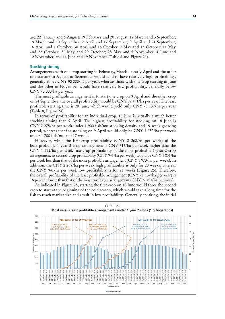
41Optimizing crop arrangements for better performance
are: 22 January and 6 August; 19 February and 20 August; 12 March and 3 September; 19 March and 10 September; 2 April and 17 September; 9 April and 24 September; 16 April and 1 October; 30 April and 18 October; 7 May and 15 October; 14 May and 22 October; 21 May and 29 October; 28 May and 5 November; 4 June and 12 November; and 11 June and 19 November (Table 8 and Figure 24).
Stocking timingArrangements with one crop starting in February, March or early April and the other one starting in August or September would tend to have relatively high profitability, generally above CNY 90 000/ha per year, whereas those with one crop starting in June and the other in November would have relatively low profitability, generally below CNY 70 000/ha per year.
The most profitable arrangement is to start one crop on 9 April and the other crop on 24 September; the overall profitability would be CNY 92 491/ha per year. The least profitable starting time is 28 June, which would yield only CNY 78 137/ha per year (Table 8; Figure 24).
In terms of profitability for an individual crop, 18 June is actually a much better stocking timing than 9 April. The highest profitability for stocking on 18 June is CNY 2 275/ha per week under 1 900 fish/mu stocking density and 19-week growing period, whereas that for stocking on 9 April would only be CNY 1 630/ha per week under 1 700 fish/mu and 17 weeks.
However, while the first-crop profitability (CNY 2 268/ha per week) of the least profitable 1-year-2-crop arrangement is CNY 716/ha per week higher than the CNY 1 552/ha per week first-crop profitability of the most profitable 1-year-2-crop arrangement, its second-crop profitability (CNY 941/ha per week) would be CNY 1 031/ha per week less than that of the most profitable arrangement (CNY 1 973/ha per week). In addition, the CNY 2 268/ha per week high profitability is only for 20 weeks, whereas the CNY 941/ha per week low profitability is for 28 weeks (Figure 25). Therefore, the overall profitability of the least profitable arrangement (CNY 78 137/ha per year) is 16 percent lower than that of the most profitable arrangement (CNY 92 491/ha per year).
As indicated in Figure 25, starting the first crop on 18 June would force the second crop to start at the beginning of the cold season, which would take a long time for the fish to reach market size and result in low profitability. Generally speaking, the initial
Reference is always at the end but before the Appendices.
Maxprofit(1stcrop):1700fish/mu,22weeks554g,1552CNY/ha/week
Maxprofit(2ndcrop):2000fish/mu,26weeks530g,1973CNY/ha/week
Minprofit (1stcrop):2000fish/mu,20weeks530g,2268CNY/ha/week
Minprofit (2ndcrop):1600fish/mu,28weeks532g,941CNY/ha/week
-
10
20
30
40
50
60
70
-
100
200
300
400
500
600
700
800
900
01/01/1sty
ear
15/01/1sty
ear
29/01/1sty
ear
12/02/1sty
ear
26/02/1sty
ear
12/03/1sty
ear
26/03/1sty
ear
09/04/1sty
ear
23/04/1sty
ear
07/05/1sty
ear
21/05/1sty
ear
04/06/1sty
ear
18/06/1sty
ear
02/07/1sty
ear
16/07/1sty
ear
30/07/1sty
ear
13/08/1sty
ear
27/08/1sty
ear
10/09/1sty
ear
24/09/1sty
ear
08/10/1sty
ear
22/10/1sty
ear
05/11/1sty
ear
19/11/1sty
ear
03/12/1sty
ear
17/12/1sty
ear
01/01/2ndyear
15/01/2ndyear
29/01/2ndyear
12/02/2ndyear
26/02/2ndyear
12/03/2ndyear
26/03/2ndyear
09/04/2ndyear
23/04/2ndyear
07/05/2ndyear
21/05/2ndyear
04/06/2ndyear
18/06/2ndyear
02/07/2ndyear
16/07/2ndyear
30/07/2ndyear
13/08/2ndyear
27/08/2ndyear
10/09/2ndyear
24/09/2ndyear
08/10/2ndyear
22/10/2ndyear
05/11/2ndyear
19/11/2ndyear
03/12/2ndyear
17/12/2ndyear
Jan Feb Mar Apr May Jun Jul Aug Sep Oct Nov Dec Jan Feb Mar Apr May Jun Jul Aug Sep Oct Nov Dec
Bars:w
aterte
mperature(ºC)
Dotte
dlines:size
offish
(g)
Stockingtiming
Watertemperature
Max profit:92491CNY/ha/year Minprofit:78137CNY/ha/year
FIGURE 25Most versus least profitable arrangements under 1 year 2 crops (1 g fingerlings)
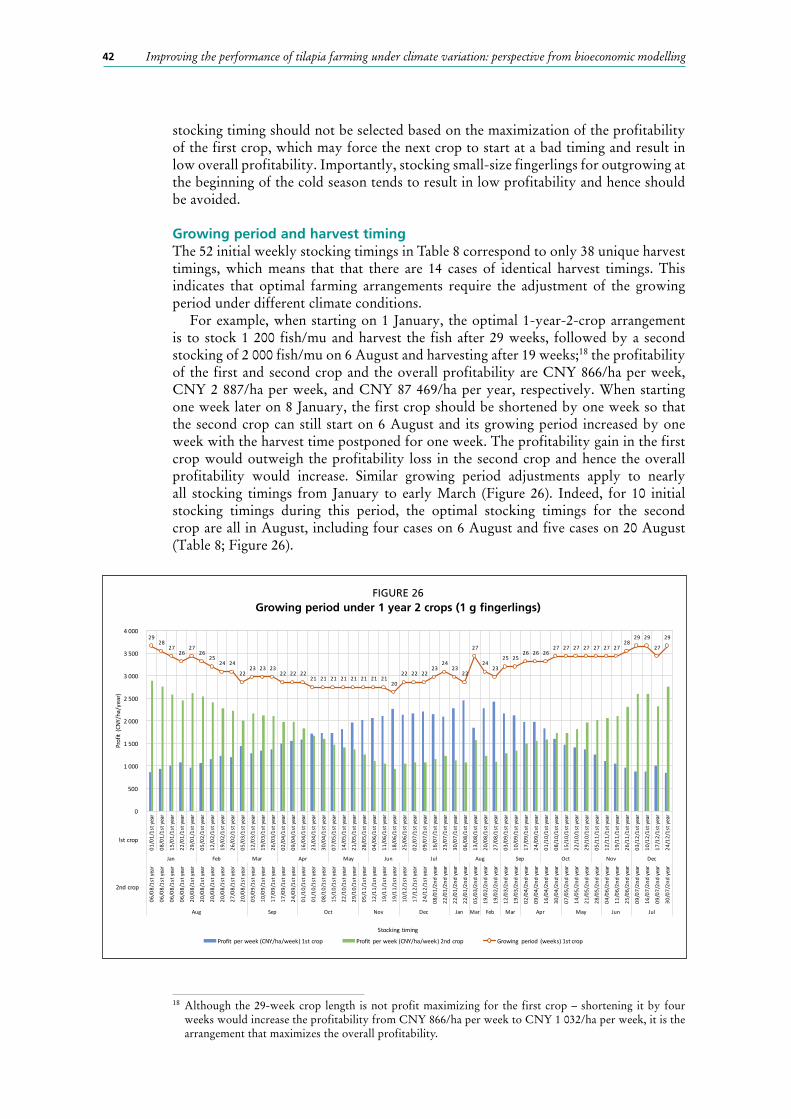
Improving the performance of tilapia farming under climate variation: perspective from bioeconomic modelling42
stocking timing should not be selected based on the maximization of the profitability of the first crop, which may force the next crop to start at a bad timing and result in low overall profitability. Importantly, stocking small-size fingerlings for outgrowing at the beginning of the cold season tends to result in low profitability and hence should be avoided.
Growing period and harvest timingThe 52 initial weekly stocking timings in Table 8 correspond to only 38 unique harvest timings, which means that that there are 14 cases of identical harvest timings. This indicates that optimal farming arrangements require the adjustment of the growing period under different climate conditions.
For example, when starting on 1 January, the optimal 1-year-2-crop arrangement is to stock 1 200 fish/mu and harvest the fish after 29 weeks, followed by a second stocking of 2 000 fish/mu on 6 August and harvesting after 19 weeks;18 the profitability of the first and second crop and the overall profitability are CNY 866/ha per week, CNY 2 887/ha per week, and CNY 87 469/ha per year, respectively. When starting one week later on 8 January, the first crop should be shortened by one week so that the second crop can still start on 6 August and its growing period increased by one week with the harvest time postponed for one week. The profitability gain in the first crop would outweigh the profitability loss in the second crop and hence the overall profitability would increase. Similar growing period adjustments apply to nearly all stocking timings from January to early March (Figure 26). Indeed, for 10 initial stocking timings during this period, the optimal stocking timings for the second crop are all in August, including four cases on 6 August and five cases on 20 August (Table 8; Figure 26).
18 Although the 29-week crop length is not profit maximizing for the first crop – shortening it by four weeks would increase the profitability from CNY 866/ha per week to CNY 1 032/ha per week, it is the arrangement that maximizes the overall profitability.
2928
2726
2726
2524 24
2223 23 23
22 22 2221 21 21 21 21 21 21 21
20
22 22 2223
2423
22
27
2423
25 2526 26 26
27 27 27 27 27 27 2728
29 29
27
29
06/08/1styear
06/08/1styear
06/08/1styear
06/08/1styear
20/08/1styear
20/08/1styear
20/08/1styear
20/08/1styear
27/08/1styear
20/08/1styear
03/09/1styear
10/09/1styear
17/09/1styear
17/09/1styear
24/09/1styear
01/10/1styear
01/10/1styear
08/10/1styear
15/10/1styear
22/10/1styear
29/10/1styear
05/11/1styear
12/11/1styear
19/11/1styear
19/11/1styear
10/12/1styear
17/12/1styear
24/12/1styear
08/01/2n
dyear
22/01/2n
dyear
22/01/2n
dyear
22/01/2n
dyear
05/03/2n
dyear
19/02/2n
dyear
19/02/2n
dyear
12/03/2n
dyear
19/03/2n
dyear
02/04/2n
dyear
09/04/2n
dyear
16/04/2n
dyear
30/04/2n
dyear
07/05/2n
dyear
14/05/2n
dyear
21/05/2n
dyear
28/05/2n
dyear
04/06/2n
dyear
11/06/2n
dyear
25/06/2n
dyear
09/07/2n
dyear
16/07/2n
dyear
09/07/2n
dyear
30/07/2n
dyear
Aug Sep Oct Nov Dec Jan Mar Feb Mar Apr May Jun Jul
0
500
1000
1500
2000
2500
3000
3500
4000
01/01/1styear
08/01/1styear
15/01/1styear
22/01/1styear
29/01/1styear
05/02/1styear
12/02/1styear
19/02/1styear
26/02/1styear
05/03/1styear
12/03/1styear
19/03/1styear
26/03/1styear
02/04/1styear
09/04/1styear
16/04/1styear
23/04/1styear
30/04/1styear
07/05/1styear
14/05/1styear
21/05/1styear
28/05/1styear
04/06/1styear
11/06/1styear
18/06/1styear
25/06/1styear
02/07/1styear
09/07/1styear
16/07/1styear
23/07/1styear
30/07/1styear
06/08/1styear
13/08/1styear
20/08/1styear
27/08/1styear
03/09/1styear
10/09/1styear
17/09/1styear
24/09/1styear
01/10/1styear
08/10/1styear
15/10/1styear
22/10/1styear
29/10/1styear
05/11/1styear
12/11/1styear
19/11/1styear
26/11/1styear
03/12/1styear
10/12/1styear
17/12/1styear
24/12/1styear
Jan Feb Mar Apr May Jun Jul Aug Sep Oct Nov Dec
2ndcrop
Profit(CNY
/ha/year)
!stcrop
Profit perweek(CNY/ha/week)1stcrop Profit perweek(CNY/ha/week)2ndcrop Growing period (weeks)1stcrop
Stockingtiming
FIGURE 26Growing period under 1 year 2 crops (1 g fingerlings)
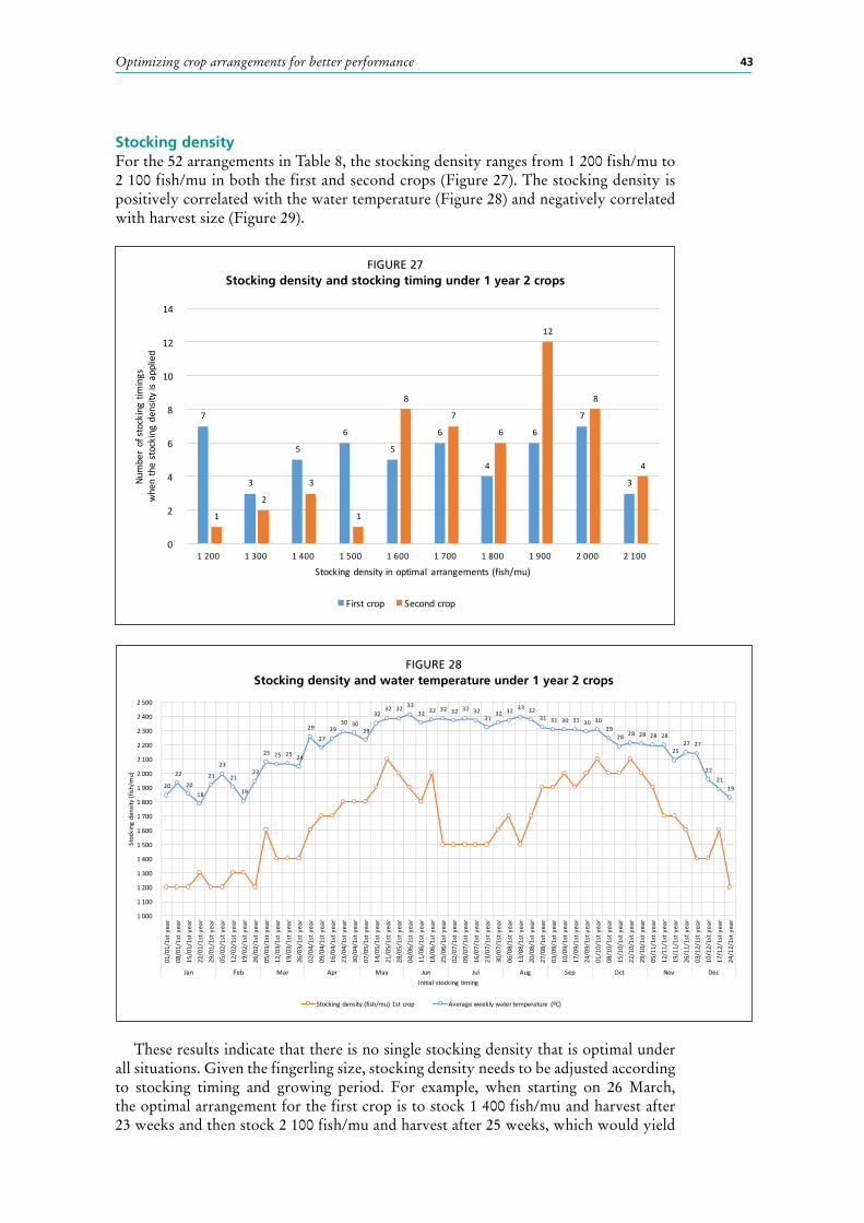
43Optimizing crop arrangements for better performance
Stocking densityFor the 52 arrangements in Table 8, the stocking density ranges from 1 200 fish/mu to 2 100 fish/mu in both the first and second crops (Figure 27). The stocking density is positively correlated with the water temperature (Figure 28) and negatively correlated with harvest size (Figure 29).
These results indicate that there is no single stocking density that is optimal under all situations. Given the fingerling size, stocking density needs to be adjusted according to stocking timing and growing period. For example, when starting on 26 March, the optimal arrangement for the first crop is to stock 1 400 fish/mu and harvest after 23 weeks and then stock 2 100 fish/mu and harvest after 25 weeks, which would yield
7
3
5
6
5
6
4
6
7
3
1
2
3
1
8
7
6
12
8
4
0
2
4
6
8
10
12
14
1200 1300 1400 1500 1600 1700 1800 1900 2000 2100
Numberofstockingtimings
whenthestockingdensityisapplied
Stockingdensityinoptimal arrangements(fish/mu)
Firstcrop Secondcrop
FIGURE 27Stocking density and stocking timing under 1 year 2 crops
20
22
2018
21
23
21
19
22
25 25 25 24
29
2729
30 3029
3232 32 33
32 3232 32 32 32
3132 32
33 3231 31 30 31 30 30
2928 28 28 28 28
2527 27
2221
19
1000
1100
1200
1300
1400
1500
1600
1700
1800
1900
2000
2100
2200
2300
2400
2500
01/01/1styear
08/01/1styear
15/01/1styear
22/01/1styear
29/01/1styear
05/02/1styear
12/02/1styear
19/02/1styear
26/02/1styear
05/03/1styear
12/03/1styear
19/03/1styear
26/03/1styear
02/04/1styear
09/04/1styear
16/04/1styear
23/04/1styear
30/04/1styear
07/05/1styear
14/05/1styear
21/05/1styear
28/05/1styear
04/06/1styear
11/06/1styear
18/06/1styear
25/06/1styear
02/07/1styear
09/07/1styear
16/07/1styear
23/07/1styear
30/07/1styear
06/08/1styear
13/08/1styear
20/08/1styear
27/08/1styear
03/09/1styear
10/09/1styear
17/09/1styear
24/09/1styear
01/10/1styear
08/10/1styear
15/10/1styear
22/10/1styear
29/10/1styear
05/11/1styear
12/11/1styear
19/11/1styear
26/11/1styear
03/12/1styear
10/12/1styear
17/12/1styear
24/12/1styear
Jan Feb Mar Apr May Jun Jul Aug Sep Oct Nov Dec
Stockingdensity(fish/mu)
Initialstockingtiming
Stockingdensity(fish/mu)1stcrop Averageweeklywatertemperature (ºC)
FIGURE 28Stocking density and water temperature under 1 year 2 crops

Improving the performance of tilapia farming under climate variation: perspective from bioeconomic modelling44
CNY 91 004/ha per year of profit (CNY 1 368/ha per week and CNY 2 104/ha per week for the first and second crop, respectively). When the starting date is moved forward by one week to 2 April, if the same arrangements of stocking density and growing period are used, the overall profit would be CNY 60 268/ha per year only (CNY 1 419/ha per week and CNY 918/ha per week for the first and second crop, respectively). The much lower profitability of the second crop is due to fish weighing under 500 g at harvest size and hence the lower farmgate price. In order to allow the second crop to produce fish with a desirable size, the farmer can reduce the stocking density and/or increase the growing period of the second crop.
Suppose the farmer reduces the stocking density for the second crop to 1 800 fish/mu, yet keeps the growing period the same at 25 weeks, the overall profitability would be increased to CNY 81 491/ha per year (CNY 1 419/ha per week and CNY 1 705/ha per week for the first and second crop, respectively).
Suppose the first crop is shortened by one week to 22 weeks and the second increased to 26 weeks; accordingly, the stocking density in the second crop would need to be reduced to 1 900 fish/mu in order to keep the fish biomass within the 16 000 kg/ha limit. Under this situation, the overall profitability would be increased to CNY 90 920/ha per year (CNY 1 488/ha per week and CNY 1 972/ha per week for the first and second crop, respectively). It should be noted that shortening the growing period of the first crop would increase its profitability from CNY 1 419 to CNY 1 488/ha per week.
However, the CNY 90 920/ha per year overall profit is still not the maximum profitability when starting on 2 April. Because of the shortened growing period, the stocking density for the first crop can be increased from 1 400 to 1 600 fish/mu, which would increase the first crop profitability to CNY 1 502/ha per week and the overall profitability to CNY 91 270/ha per year.
For a crop starting in the low temperature season (from December to February), the stocking density tends to be relatively low with a relatively long growing period and large harvest size under the optimal arrangement (Figure 28). For example, when stocking on 5 February, the first crop arrangement that would maximize the overall profitability is to stock 1 200 fish/mu and harvest 698 g fish after 26 weeks (Table 8). The profitability of this first crop arrangement would generate a profit of
595609
623632610611617
636622
607
580569
559561541
527532521515505506
518537544531
603602609611615
630632
603
636
611
580569561
541527521515
505506518
537544546554
571
594598
01/0
1/1s
tyea
r
08/0
1/1s
tyea
r
15/0
1/1s
tyea
r
22/0
1/1s
tyea
r
29/0
1/1s
tyea
r
05/0
2/1s
tyea
r
12/0
2/1s
tyea
r
19/0
2/1s
tyea
r
26/0
2/1s
tyea
r
05/0
3/1s
tyea
r
12/0
3/1s
tyea
r
19/0
3/1s
tyea
r
26/0
3/1s
tyea
r
02/0
4/1s
tyea
r
09/0
4/1s
tyea
r
16/0
4/1s
tyea
r
23/0
4/1s
tyea
r
30/0
4/1s
tyea
r
07/0
5/1s
tyea
r
14/0
5/1s
tyea
r
21/0
5/1s
tyea
r
28/0
5/1s
tyea
r
04/0
6/1s
tyea
r
11/0
6/1s
tyea
r
18/0
6/1s
tyea
r
25/0
6/1s
tyea
r
02/0
7/1s
tyea
r
09/0
7/1s
tyea
r
16/0
7/1s
tyea
r
23/0
7/1s
tyea
r
30/0
7/1s
tyea
r
06/0
8/1s
tyea
r
13/0
8/1s
tyea
r
20/0
8/1s
tyea
r
27/0
8/1s
tyea
r
03/0
9/1s
tyea
r
10/0
9/1s
tyea
r
17/0
9/1s
tyea
r
24/0
9/1s
tyea
r
01/1
0/1s
tyea
r
08/1
0/1s
tyea
r
15/1
0/1s
tyea
r
22/1
0/1s
tyea
r
29/1
0/1s
tyea
r
05/1
1/1s
tyea
r
12/1
1/1s
tyea
r
19/1
1/1s
tyea
r
26/1
1/1s
tyea
r
03/1
2/1s
tyea
r
10/1
2/1s
tyea
r
17/1
2/1s
tyea
r
24/1
2/1s
tyea
r
Jan Feb Mar Apr May Jun Jul Aug Sep Oct Nov Dec
0
500
1000
1500
2000
2500
01/0
1/1s
tyea
r
08/0
1/1s
tyea
r
15/0
1/1s
tyea
r
22/0
1/1s
tyea
r
29/0
1/1s
tyea
r
05/0
2/1s
tyea
r
12/0
2/1s
tyea
r
19/0
2/1s
tyea
r
26/0
2/1s
tyea
r
05/0
3/1s
tyea
r
12/0
3/1s
tyea
r
19/0
3/1s
tyea
r
26/0
3/1s
tyea
r
02/0
4/1s
tyea
r
09/0
4/1s
tyea
r
16/0
4/1s
tyea
r
23/0
4/1s
tyea
r
30/0
4/1s
tyea
r
07/0
5/1s
tyea
r
14/0
5/1s
tyea
r
21/0
5/1s
tyea
r
28/0
5/1s
tyea
r
04/0
6/1s
tyea
r
11/0
6/1s
tyea
r
18/0
6/1s
tyea
r
25/0
6/1s
tyea
r
02/0
7/1s
tyea
r
09/0
7/1s
tyea
r
16/0
7/1s
tyea
r
23/0
7/1s
tyea
r
30/0
7/1s
tyea
r
06/0
8/1s
tyea
r
13/0
8/1s
tyea
r
20/0
8/1s
tyea
r
27/0
8/1s
tyea
r
03/0
9/1s
tyea
r
10/0
9/1s
tyea
r
17/0
9/1s
tyea
r
24/0
9/1s
tyea
r
01/1
0/1s
tyea
r
08/1
0/1s
tyea
r
15/1
0/1s
tyea
r
22/1
0/1s
tyea
r
29/1
0/1s
tyea
r
05/1
1/1s
tyea
r
12/1
1/1s
tyea
r
19/1
1/1s
tyea
r
26/1
1/1s
tyea
r
03/1
2/1s
tyea
r
10/1
2/1s
tyea
r
17/1
2/1s
tyea
r
24/1
2/1s
tyea
r
Jan Feb Mar Apr May Jun Jul Aug Sep Oct Nov Dec
2ndcrop
Aver
agestoc
king
den
sity
(fish
/mu)
1stcrop
Averagestockingdensity(fish/mu) Averageharvestsize(g)
Stocking timing
FIGURE 29Stocking density and harvest size under 1 year 2 crops

45Optimizing crop arrangements for better performance
CNY 1 058/ha per week, which is lower than the maximum first crop profitability (CNY 1 375/ha per week) achievable by stocking 1 400 fish/mu and harvesting 503 g fish after 21 weeks. However, having a 26-week first crop would allow the second crop to have more opportune stocking timing and growing period, and the profitability gain in the second crop would exceed the profitability loss in the first crop. Given the 26-week growing period, 1 400 fish/mu is not optimal; it would be better to lower it to 1 200 fish/mu so as to mitigate the inefficiency caused by the overly long growing period.
ProductivityWith the fish biomass limit imposed in the model, the largest productivity allowed is 16 000 kg/ha per crop, which means 32 000 kg/ha per year under a 1-year-2-crop arrangement. For the 52 initial stocking timings, the overall productivity ranges from 27 147 kg/ha per year (stocking on 25 June) to 31 132 kg/ha per year (stocking on 21 May), with most of them below 30 000 kg/ha per year (Figure 30). This means that the fish biomass upper bound (16 000 kg/ha per crop) is not binding under many occasions. As indicated in Figure 31, for nearly all of the 52 initial stocking timings, the 16 000 fish biomass limit is binding in one crop but not in the other.
For example, when starting on 9 April, the optimal first crop arrangement under 1 year 2 crops is to stock 1 700 fish/mu and harvest 554 g fish after 22 weeks (Table 8). The first crop production is 14 132 kg/ha/crop. Increasing the stocking density from 1 700 fish/mu to 2 000 fish/mu would reduce the harvest size to 507 g (still a desirable size) yet increase the yield to 15 217 kg/ha per crop. The profit of the first crop, however, would be reduced from CNY 1 552/ha per week to CNY 1 519/ha per week.
On the other hand, the optimal arrangement for the second crop, which is to stock 2 000 fish/mu on 24 September and harvest 530 g fish after 26 weeks, would have the production (15 903 kg/ha per crop) bound by the fish biomass limit. That is, increasing the stocking density to 2 100 fish/mu is not possible in the model because the fish biomass at harvest would exceed the 16 000 fish/mu upper bound.
More general 1-year-2-crop arrangementsUnder a 1-year-2-crop arrangement, the crop length of the two crops (including the time for pond preparation) needs to add up to 52 weeks. This could force the farmer to adopt an inefficient arrangement in one or another or both crops.
75000
77000
79000
81000
83000
85000
87000
89000
91000
93000
95000
25000
26000
27000
28000
29000
30000
31000
32000
33000
34000
35000
01/01/1styear
08/01/1styear
15/01/1styear
22/01/1styear
29/01/1styear
05/02/1styear
12/02/1styear
19/02/1styear
26/02/1styear
05/03/1styear
12/03/1styear
19/03/1styear
26/03/1styear
02/04/1styear
09/04/1styear
16/04/1styear
23/04/1styear
30/04/1styear
07/05/1styear
14/05/1styear
21/05/1styear
28/05/1styear
04/06/1styear
11/06/1styear
18/06/1styear
25/06/1styear
02/07/1styear
09/07/1styear
16/07/1styear
23/07/1styear
30/07/1styear
06/08/1styear
13/08/1styear
20/08/1styear
27/08/1styear
03/09/1styear
10/09/1styear
17/09/1styear
24/09/1styear
01/10/1styear
08/10/1styear
15/10/1styear
22/10/1styear
29/10/1styear
05/11/1styear
12/11/1styear
19/11/1styear
26/11/1styear
03/12/1styear
10/12/1styear
17/12/1styear
24/12/1styear
Jan Feb Mar Apr May Jun Jul Aug Sep Oct Nov Dec
Totalprofit(CN
Y/ha/year)
Totalproduction(kg/ha/year)
Initialstockingtiming
Totalproduction (kg/ha/year) Totalprofit (CNY/ha/year)
FIGURE 30Overall productivity and profitability under 1 year 2 crops

Improving the performance of tilapia farming under climate variation: perspective from bioeconomic modelling46
In order to relax the constraint, arrangements of 2 years 4 crops are simulated. A 2-year-4-crop arrangement is on average one year and two crops, but the total crop length of any two of the four crops does not need to add up to 52 weeks, even though the total crop length of the four crops would need to add up to 104 weeks.
The results indicate that 2 years 4 crops would have slightly better profitability for some initial stocking timing, yet the same profitability for other initial stocking timing (Figure 32). For example, when starting on 18 June, the profitability for 2 years 4 crops would be CNY 79 412/ha per year, greater than the CNY 78 137/ha per year profitability under 1 year 2 crops. On the other hand, when starting on 9 April, the
0
4000
8000
12000
16000
20000
24000
28000
32000
36000
40000
44000
48000
52000
56000
60000
64000
01/0
1/1s
tyea
r
08/0
1/1s
tyea
r
15/0
1/1s
tyea
r
22/0
1/1s
tyea
r
29/0
1/1s
tyea
r
05/0
2/1s
tyea
r
12/0
2/1s
tyea
r
19/0
2/1s
tyea
r
26/0
2/1s
tyea
r
05/0
3/1s
tyea
r
12/0
3/1s
tyea
r
19/0
3/1s
tyea
r
26/0
3/1s
tyea
r
02/0
4/1s
tyea
r
09/0
4/1s
tyea
r
16/0
4/1s
tyea
r
23/0
4/1s
tyea
r
30/0
4/1s
tyea
r
07/0
5/1s
tyea
r
14/0
5/1s
tyea
r
21/0
5/1s
tyea
r
28/0
5/1s
tyea
r
04/0
6/1s
tyea
r
11/0
6/1s
tyea
r
18/0
6/1s
tyea
r
25/0
6/1s
tyea
r
02/0
7/1s
tyea
r
09/0
7/1s
tyea
r
16/0
7/1s
tyea
r
23/0
7/1s
tyea
r
30/0
7/1s
tyea
r
06/0
8/1s
tyea
r
13/0
8/1s
tyea
r
20/0
8/1s
tyea
r
27/0
8/1s
tyea
r
03/0
9/1s
tyea
r
10/0
9/1s
tyea
r
17/0
9/1s
tyea
r
24/0
9/1s
tyea
r
01/1
0/1s
tyea
r
08/1
0/1s
tyea
r
15/1
0/1s
tyea
r
22/1
0/1s
tyea
r
29/1
0/1s
tyea
r
05/1
1/1s
tyea
r
12/1
1/1s
tyea
r
19/1
1/1s
tyea
r
26/1
1/1s
tyea
r
03/1
2/1s
tyea
r
10/1
2/1s
tyea
r
17/1
2/1s
tyea
r
24/1
2/1s
tyea
r
Jan Feb Mar Apr May Jun Jul Aug Sep Oct Nov Dec
Prod
uctiv
ity(
kg/h
a/cr
op)o
rpro
fitab
ility
(CNY
/ha/
crop
)
Initialstockingtiming
Totalproduction1stcrop(kg/ha/crop) Totalproduction2ndcrop(kg/ha/crop) Totalprofit1stcrop(CNY/ha/crop) Totalprofit2ndcrop(CNY/ha/crop)
FIGURE 31Productivity and profitability by crop under 1 year 2 crops
70000
75000
80000
85000
90000
95000
01/01/1s
tyear
08/01/1s
tyear
15/01/1s
tyear
22/01/1s
tyear
29/01/1s
tyear
05/02/1s
tyear
12/02/1s
tyear
19/02/1s
tyear
26/02/1s
tyear
05/03/1s
tyear
12/03/1s
tyear
19/03/1s
tyear
26/03/1s
tyear
02/04/1s
tyear
09/04/1s
tyear
16/04/1s
tyear
23/04/1s
tyear
30/04/1s
tyear
07/05/1s
tyear
14/05/1s
tyear
21/05/1s
tyear
28/05/1s
tyear
04/06/1s
tyear
11/06/1s
tyear
18/06/1s
tyear
25/06/1s
tyear
02/07/1s
tyear
09/07/1s
tyear
16/07/1s
tyear
23/07/1s
tyear
30/07/1s
tyear
06/08/1s
tyear
13/08/1s
tyear
20/08/1s
tyear
27/08/1s
tyear
03/09/1s
tyear
10/09/1s
tyear
17/09/1s
tyear
24/09/1s
tyear
01/10/1s
tyear
08/10/1s
tyear
15/10/1s
tyear
22/10/1s
tyear
29/10/1s
tyear
05/11/1s
tyear
12/11/1s
tyear
19/11/1s
tyear
26/11/1s
tyear
03/12/1s
tyear
10/12/1s
tyear
17/12/1s
tyear
24/12/1s
tyear
Jan Feb Mar Apr May Jun Jul Aug Sep Oct Nov Dec
CNY/ha
/yea
r
InitialstockingtimingProfitabilty for1year2crops (CNY/ha/year) Profitabilty for2year4crops (CNY/ha/year)
FIGURE 32Profitability – 2 years 4 crops versus 1 year 2 crops
47Optimizing crop arrangements for better performance
profitability for 2 years 4 crops would be the same as that for 1 year 2 crops, which means that the optimal arrangement for 2 years 4 crops would be a replicate of that for 1 year 2 crops.
SummaryThe results in Table 8 are optimal arrangements that give the maximum profitability under 1-year-2-crop arrangements for different initial stocking timings. When farmers have freedom to select the initial stocking timing, they should choose an initial stocking timing (e.g. 9 April) that gives relatively high profitability and follow the arrangements described in Table 8 to realize the high profitability.
However, when farmers have to start on a less opportune stocking timing, they should not follow the arrangement for the stocking timing described in Table 8, which would keep the operation trapped in a low-profit arrangement. Instead, farmers should arrange initial crops in such a way as to allow the selection of a more opportune stocking timing.
For example, suppose that for some reason (e.g. the availability of fingerlings or other materials or financial resources) a farmer has to postpone the initial stocking timing to 23 April (two weeks later than the optimal stocking timing on 9 April), it is not advisable to follow the corresponding arrangement described in Table 8 (i.e. a 1 800 fish/mu, 21-week first crop and a 1 900 fish/mu, 27-week second crop) because it would result in a profitability of CNY 88 078/ha per year. Instead, the farmer can adopt a 50-week cycle (i.e. a 1 500 fish/mu, 20-week first crop and a 2 000 fish/mu, 26-week second crop), which would generate CNY 91 375 of total profit and allow the next cycle to start on the optimal stocking timing on 9 April.
4.3 HARVESTING SMALLER SIZE FISHIn China, tilapia below 500 g are usually considered small-size fish sold at a discounted price. However, consumers in some countries (the Philippines, for example) prefer smaller tilapia, around 250 g. Experts from the industry and academics suggest that farming relatively small-size tilapia could improve profitability,19 especially when there is not much price discrepancy between small- and large-size fish.
It is argued that farming relatively small-size fish could shorten the production cycle and hence allow farmers to profit from more crops. Also, the FCR tends to be lower during the early stages of farming. However, farming small-size fish tends to be inefficient in the use of fingerlings. Additionally, harvesting at a small size may miss the fast growing part of the tilapia cycle. This especially matters for GIFT strains, which tend to show advantages at the later stages. In light of this background, the advanced bioeconomic model is used to examine whether it would be more profitable to farm relatively small-size fish.
Premium price for large-size fishThe harvest size in all situations in Table 8 is more than 500 g. This indicates that when, as is the case in most places in China, there is a price premium for 500–1 000 g fish (CNY 9.89/kg) compared with 250–500 g fish (CNY 7.95/kg), harvesting fish below 500 g would be suboptimal in a 1-year-2-crop arrangement.
No price discrepancy between small- and large-size fishWhat if there were no price discrepancy between small- and large-size fish? Indeed, small-size fish may be preferred for various reasons. In the Philippines, for instance,
19 See, for example, the article Could aquaculture solve Africa’s fishing crisis?, published by The Guardian on 5 June 2013. Available at: https://www.theguardian.com/global-development-professionals-network/2013/jun/05/aquaculture-africa-fishing-crisis-marine.

Improving the performance of tilapia farming under climate variation: perspective from bioeconomic modelling48
many households prefer buying 250–300 g tilapia so that each family member can be served one whole fish at dinner. In Yunnan province, in China, restaurants like to use 250–300 g tilapia to prepare grilled fish, as they are easier to season and have more tender flesh than larger fish. In many places in Africa, 250 g and smaller fish are often sold in pieces by which the equivalent price in weight could be higher than larger fish.
In order to examine optimal farming arrangements under no price discrepancy between small- and large-size fish, the baseline assumption is modified to let the price of 250–500 g fish be the same as that of 500–1 000 g fish (i.e. CNY 9.89/kg). Under this situation, the simulation results indicate that harvesting small-size fish could be more profitable.
1 year 2 cropsAs indicated in Figure 33, the overall profitability of 1 year 2 crops could be improved by farming smaller fish. For example, under the baseline situation where the price for 250–500 g fish is lower than that of 500–1 000 g, when stocking on 19 November the optimal arrangement for the first crop is to stock 1 700 fish/mu and harvest 503 g fish after 27 weeks for CNY 1 057/ha per week profitability. The 27-week growing period is necessary – harvesting small-size fish at 483 g after 26 weeks would render a much lower first crop profitability (CNY 310/ha per week). When there is no price discrepancy for small fish, farmers could choose to stock 3 100 fish/mu and harvest 343 g fish after 24 weeks for a profit of CNY 1 685/ha per week, which is much higher than the baseline case. The overall profit would be CNY 87 762/ha per year compared with CNY 79 158/ha per year in the baseline case (Figure 33).
However, for many stocking timings (including those that give relatively high overall profit), the overall profitability is the same with or without price discrepancy for small fish (Figure 33). This implies that when the initial stocking timing allows a conducive growing period for both crops, harvesting small-size fish would not improve profitability under 1 year 2 crops. For example, when starting on 9 April, the optimal first crop arrangement would be to stock 1 700 fish/mu and harvest 554 g fish after 22 weeks for a production of 14 123 kg/ha per crop and a profit of CNY 1 552/ha per week. The farmer can increase the production to 15 889 kg/ha per crop by increasing
70000
75000
80000
85000
90000
95000
01/0
1/1s
tyea
r
08/0
1/1s
tyea
r
15/0
1/1s
tyea
r
22/0
1/1s
tyea
r
29/0
1/1s
tyea
r
05/0
2/1s
tyea
r
12/0
2/1s
tyea
r
19/0
2/1s
tyea
r
26/0
2/1s
tyea
r
05/0
3/1s
tyea
r
12/0
3/1s
tyea
r
19/0
3/1s
tyea
r
26/0
3/1s
tyea
r
02/0
4/1s
tyea
r
09/0
4/1s
tyea
r
16/0
4/1s
tyea
r
23/0
4/1s
tyea
r
30/0
4/1s
tyea
r
07/0
5/1s
tyea
r
14/0
5/1s
tyea
r
21/0
5/1s
tyea
r
28/0
5/1s
tyea
r
04/0
6/1s
tyea
r
11/0
6/1s
tyea
r
18/0
6/1s
tyea
r
25/0
6/1s
tyea
r
02/0
7/1s
tyea
r
09/0
7/1s
tyea
r
16/0
7/1s
tyea
r
23/0
7/1s
tyea
r
30/0
7/1s
tyea
r
06/0
8/1s
tyea
r
13/0
8/1s
tyea
r
20/0
8/1s
tyea
r
27/0
8/1s
tyea
r
03/0
9/1s
tyea
r
10/0
9/1s
tyea
r
17/0
9/1s
tyea
r
24/0
9/1s
tyea
r
01/1
0/1s
tyea
r
08/1
0/1s
tyea
r
15/1
0/1s
tyea
r
22/1
0/1s
tyea
r
29/1
0/1s
tyea
r
05/1
1/1s
tyea
r
12/1
1/1s
tyea
r
19/1
1/1s
tyea
r
26/1
1/1s
tyea
r
03/1
2/1s
tyea
r
10/1
2/1s
tyea
r
17/1
2/1s
tyea
r
24/1
2/1s
tyea
r
Jan Feb Mar Apr May Jun Jul Aug Sep Oct Nov Dec
Prof
itabi
lity
(CNY
/ha/
year
)
Initialstockingtiming
Lowprice forsmall fish Nopricediscrepancyforsmall fish
FIGURE 33Overall profitability of 1 year 2 crops under no price discrepancy for small fish

49Optimizing crop arrangements for better performance
the stocking density to 2 200 fish/mu and harvesting 482 g fish after 22 weeks. The profit would nevertheless be reduced to CNY 1 492/ha per week, even with no price discrepancy between 250–500 g and 500–1 000 g fish.
In summary, under a 1-year-2-crop arrangement with no price discrepancy between small- and large-size fish, harvesting small fish could increase the profit when it would take an inefficiently long growing period to grow fish above 500 g; however, harvesting smaller fish under higher stocking density could be technically efficient (i.e. increasing productivity) yet economically inefficient (i.e. reducing profitability).
1 year 3 cropsGiven no price discrepancy between small- and large-size fish, farmers can shorten the growing period and harvest small-size fish for more than two crops a year. However, when 1 g fingerlings are stocked, it is not possible to grow fish above 250 g in all the three crops under a 1-year-3-crop arrangement. Allowing for six weeks that is needed for pond preparation (two weeks per crop), a 1-year-3-crop arrangement would have an average duration of 15 weeks. Though it is possible to grow fish over 250 g in 15 weeks when the temperature is favourable, the growth during the low temperature season would take about 20 weeks.
2 years 5 crops When examining 2-year-5-crop arrangements, all the 2-year-5-crop arrangements that maximize the overall profitability for the first two crops are identified, and then among these arrangements finding the cases that maximize the overall profitability for all the five crops. Although the arrangements identified as such (Table 9A and 9B) may not be the optimal 2-year-5-crop arrangements that maximize the overall profitability for each of the 52 stocking timings,20 they are sufficient to show that given no price discrepancy between small- and large-size fish, harvesting small-size fish (250–500 g) through 2 years 5 crops would be more profitable than harvesting large-size fish (over 500 g) through 1 year 2 crops (Figure 34).
20 It is difficult to simulate the large number of all the feasible 2-year-5-crop arrangements comprehensively.
117 533
123 586
92 491 92 491
0
8 000
16 000
24 000
32 000
40 000
48 000
56 000
64 000
72 000
80 000
0
15 000
30 000
45 000
60 000
75 000
90 000
105 000
120 000
135 000
150 000
01/0
1/1s
t yea
r
08/0
1/1s
t yea
r
15/0
1/1s
t yea
r
22/0
1/1s
t yea
r
29/0
1/1s
t yea
r
05/0
2/1s
t yea
r
12/0
2/1s
t yea
r
19/0
2/1s
t yea
r
26/0
2/1s
t yea
r
05/0
3/1s
t yea
r
12/0
3/1s
t yea
r
19/0
3/1s
t yea
r
26/0
3/1s
t yea
r
02/0
4/1s
t yea
r
09/0
4/1s
t yea
r
16/0
4/1s
t yea
r
23/0
4/1s
t yea
r
30/0
4/1s
t yea
r
07/0
5/1s
t yea
r
14/0
5/1s
t yea
r
21/0
5/1s
t yea
r
28/0
5/1s
t yea
r
04/0
6/1s
t yea
r
11/0
6/1s
t yea
r
18/0
6/1s
t yea
r
25/0
6/1s
t yea
r
02/0
7/1s
t yea
r
09/0
7/1s
t yea
r
16/0
7/1s
t yea
r
23/0
7/1s
t yea
r
30/0
7/1s
t yea
r
06/0
8/1s
t yea
r
13/0
8/1s
t yea
r
20/0
8/1s
t yea
r
27/0
8/1s
t yea
r
03/0
9/1s
t yea
r
10/0
9/1s
t yea
r
17/0
9/1s
t yea
r
24/0
9/1s
t yea
r
01/1
0/1s
t yea
r
08/1
0/1s
t yea
r
15/1
0/1s
t yea
r
22/1
0/1s
t yea
r
29/1
0/1s
t yea
r
05/1
1/1s
t yea
r
12/1
1/1s
t yea
r
19/1
1/1s
t yea
r
26/1
1/1s
t yea
r
03/1
2/1s
t yea
r
10/1
2/1s
t yea
r
17/1
2/1s
t yea
r
24/1
2/1s
t yea
r
Jan Feb Mar Apr May Jun Jul Aug Sep Oct Nov Dec
Prod
uctiv
ity (k
g/ha
/yea
r)
Prof
itabi
lity
(CNY
/ha/
year
)
Initial stocking timing
Productivity under 2 years 5 crops (kg/ha/year) Productivity under 1 year 2 crops (kg/ha/year)
Profitability under 2 years 5 crops (CNY/ha/year) Profitability under 1 year 2 crops (CNY/ha/year)
FIGURE 34Profitability and productivity – 2 years 5 crops versus 1 year 2 crops

Improving the performance of tilapia farming under climate variation: perspective from bioeconomic modelling50
TABLE 9A2-year-5-crop arrangements under 1 g fingerlings and no price discrepancy between small and large fish
Starting time
Stocking density (fish/mu) Growing period (weeks) Harvest size (g)
1st crop
2nd crop
3rd crop
4th crop
5th crop
Average 1st
crop 2nd crop
3rd crop
4th crop
5th crop
Average 1st crop
2nd crop
3rd crop
4th crop
5th crop
Average
Jan
01/01/1st year 3 700 4 000 2 300 4 000 2 200 3 240 19 16 25 16 18 18.8 250 252 456 251 484 312
08/01/1st year 3 800 4 100 3 100 3 900 1 900 3 360 19 16 23 16 20 18.8 251 260 342 254 559 305
15/01/1st year 3 500 4 100 3 100 2 700 2 200 3 120 18 16 23 18 19 18.8 253 260 342 345 484 321
22/01/1st year 3 400 4 100 2 700 1 700 3 900 3 160 17 16 24 21 16 18.8 251 260 386 520 272 311
29/01/1st year 3 600 3 900 3 200 1 700 3 700 3 220 17 16 23 21 17 18.8 251 270 328 520 288 308
Feb
05/02/1st year 3 800 4 200 3 900 3 800 1 900 3 520 18 15 22 17 22 18.8 263 253 272 272 557 296
12/02/1st year 3 900 4 200 3 900 1 700 4 000 3 540 17 15 22 22 18 18.8 251 253 272 554 265 288
19/02/1st year 3 700 4 200 3 900 1 700 3 000 3 300 16 15 22 21 20 18.8 251 253 272 520 354 303
26/02/1st year 3 400 4 200 3 900 2 200 2 400 3 220 15 15 22 20 22 18.8 251 253 272 424 440 308
Mar
05/03/1st year 3 400 3 900 4 100 2 400 2 700 3 300 15 15 22 20 22 18.8 251 270 260 409 390 303
12/03/1st year 3 800 4 200 4 200 2 600 3 000 3 560 16 14 22 20 22 18.8 256 251 251 395 352 290
19/03/1st year 3 500 4 200 4 200 2 600 2 700 3 440 15 14 22 20 23 18.8 250 251 251 395 391 295
26/03/1st year 3 500 4 100 2 700 3 900 2 900 3 420 15 14 25 17 23 18.8 250 259 388 272 365 299
Apr
02/04/1st year 3 300 3 900 3 100 3 900 2 600 3 360 15 14 24 17 24 18.8 250 270 343 272 409 302
09/04/1st year 4 000 4 100 4 200 4 100 2 000 3 680 16 13 22 17 26 18.8 251 251 253 257 530 283
16/04/1st year 3 800 4 200 4 100 2 100 4 100 3 660 16 13 22 21 22 18.8 251 253 260 502 260 284
23/04/1st year 3 400 4 200 4 000 2 000 4 200 3 560 16 13 22 21 22 18.8 252 252 267 529 251 286
30/04/1st year 4 000 4 000 4 200 2 500 3 100 3 560 17 14 20 19 24 18.8 251 262 250 424 342 294
May
07/05/1st year 3 200 4 000 4 200 1 600 4 200 3 440 16 14 20 22 22 18.8 251 262 250 648 251 290
14/05/1st year 3 400 3 900 3 900 1 600 4 200 3 400 16 16 18 22 22 18.8 252 272 251 657 253 295
21/05/1st year 3 700 4 000 2 600 2 000 4 100 3 280 16 18 19 19 22 18.8 252 265 343 530 260 305
28/05/1st year 4 000 4 200 1 500 2 400 4 000 3 220 16 19 22 17 20 18.8 252 251 570 444 251 310
Jun
04/06/1st year 3 400 4 200 1 500 2 200 4 200 3 100 15 19 22 18 20 18.8 251 251 570 484 250 315
11/06/1st year 3 600 4 000 2 100 2 200 4 000 3 180 15 21 20 19 19 18.8 251 265 439 484 252 312
18/06/1st year 3 900 4 200 2 200 1 900 3 500 3 140 15 21 19 22 17 18.8 251 252 411 557 252 311
25/06/1st year 4 200 3 900 1 700 3 000 3 700 3 300 15 22 21 20 16 18.8 253 272 520 354 251 303
Jul
02/07/1st year 3 900 4 100 2 400 3 000 3 600 3 400 15 22 20 20 17 18.8 270 260 409 354 271 302
09/07/1st year 3 900 4 100 2 400 3 000 2 900 3 260 14 22 20 20 18 18.8 251 260 409 354 318 307
16/07/1st year 4 200 4 200 3 200 3 000 2 400 3 400 14 22 19 20 19 18.8 251 251 330 354 372 301
23/07/1st year 4 100 4 000 3 300 3 000 2 100 3 300 14 22 18 20 20 18.8 259 251 302 354 416 303
30/07/1st year 3 900 4 200 4 100 3 000 1 800 3 400 14 22 17 20 21 18.8 270 251 251 354 474 297
Aug
06/08/1st year 3 800 4 200 3 500 2 600 3 900 3 600 14 22 18 24 16 18.8 278 253 303 409 254 291
13/08/1st year 4 100 4 200 4 100 2 000 4 000 3 680 13 22 17 26 16 18.8 251 253 257 530 251 283
20/08/1st year 4 200 4 100 3 900 2 600 2 700 3 500 13 22 17 24 18 18.8 253 260 272 409 345 296
27/08/1st year 4 200 3 900 3 900 2 600 2 400 3 400 13 21 17 24 19 18.8 252 252 272 409 380 299
Sep
03/09/1st year 3 400 3 700 3 700 3 100 2 100 3 200 15 19 17 23 20 18.8 313 250 287 342 427 313
10/09/1st year 4 000 3 700 3 700 3 100 1 800 3 260 14 19 17 23 21 18.8 262 250 287 342 497 306
17/09/1st year 3 900 3 400 4 100 2 700 1 700 3 160 16 17 16 24 21 18.8 272 251 260 386 520 311
24/09/1st year 4 000 3 200 3 700 3 900 1 700 3 300 18 16 16 22 22 18.8 265 251 286 272 554 298
Oct
01/10/1st year 4 200 3 400 1 600 4 100 3 900 3 440 19 15 21 22 17 18.8 251 251 645 260 272 295
08/10/1st year 4 000 3 500 2 200 4 100 3 300 3 420 21 15 18 22 18 18.8 265 250 479 260 321 299
15/10/1st year 4 200 3 500 2 500 4 100 2 900 3 440 21 15 17 22 19 18.8 252 250 421 260 368 298
22/10/1st year 3 900 3 300 2 000 4 200 2 800 3 240 22 15 19 20 18 18.8 272 252 531 250 369 311
29/10/1st year 4 100 3 800 2 200 4 000 2 800 3 380 22 16 19 19 18 18.8 260 251 484 252 378 304
Nov
05/11/1st year 4 200 3 400 1 900 2 400 4 200 3 220 22 16 23 19 14 18.8 251 252 558 372 251 306
12/11/1st year 4 000 4 000 2 500 2 400 3 500 3 280 22 17 21 19 15 18.8 251 251 420 372 302 305
19/11/1st year 4 200 4 100 3 000 2 400 3 000 3 340 22 17 20 19 16 18,8 251 251 354 372 355 305
26/11/1st year 4 200 4 100 4 000 3 900 1 900 3 620 22 17 18 17 20 18,8 253 257 265 251 556 288
Dec
03/12/1st year 4 100 3 700 2 000 4 000 3 600 3 480 22 16 26 16 14 18,8 260 252 530 251 292 294
10/12/1st year 3 900 3 700 2 000 4 000 3 100 3 340 21 16 26 16 15 18,8 252 252 530 251 340 301
17/12/1st year 4 200 4 000 2 300 4 000 2 700 3 440 21 16 25 16 16 18,8 252 252 456 251 394 301
24/12/1st year 4 000 4 000 2 300 4 000 2 400 3 340 20 16 25 16 17 18.8 251 252 456 251 444 307

51Optimizing crop arrangements for better performance
TABLE 9BProductivity and profitability for the 2-year-5-crop arrangements in Table 9A
Starting time
Productivity Profitability
Weekly (kg/ha/week) Annual
(kg/ha/year)
Weekly (CNY/ha/week) Annual
(CNY/ha/year) 1st crop
2nd crop
3rd crop
4th crop
5th crop
Overall 1st crop
2nd crop
3rd crop
4th crop
5th crop
Overall
Jan
01/01/1st year 662 839 583 836 798 729 37 883 1 976 2 550 2 042 2 362 3 089 2 373 123 421
08/01/1st year 680 888 636 825 724 740 38 480 1 916 2 634 2 252 2 321 2 754 2 368 123 148
15/01/1st year 663 888 636 698 760 722 37 541 1 979 2 634 2 252 1 972 2 997 2 362 122 831
22/01/1st year 674 888 602 577 884 708 36 806 2 082 2 634 2 114 1 630 3 603 2 349 122 142
29/01/1st year 713 877 629 577 842 715 37 158 2 091 2 612 2 208 1 630 3 413 2 349 122 139
Feb
05/02/1st year 749 938 663 816 661 752 39 105 1 920 2 922 2 331 2 130 2 541 2 360 122 745
12/02/1st year 772 938 663 588 794 736 38 259 2 077 2 922 2 331 1 552 3 171 2 363 122 870
19/02/1st year 775 938 663 577 724 721 37 504 2 225 2 922 2 331 1 630 2 867 2 368 123 118
26/02/1st year 753 938 663 635 660 716 37 236 2 356 2 922 2 331 1 698 2 515 2 340 121 698
Mar
05/03/1st year 754 929 665 669 658 722 37 536 2 363 3 024 2 169 1 772 2 487 2 330 121 153
12/03/1st year 811 990 660 700 659 745 38 744 2 236 3 353 2 082 1 837 2 477 2 343 121 857
19/03/1st year 774 990 660 700 633 731 38 021 2 392 3 353 2 082 1 837 2 301 2 329 121 103
26/03/1st year 773 996 582 837 635 736 38 294 2 358 3 420 1 575 2 405 2 275 2 307 119 962
Apr
02/04/1st year 728 989 614 837 614 731 38 016 2 315 3 458 1 685 2 405 2 172 2 314 120 326
09/04/1st year 836 1 028 664 832 568 751 39 055 2 362 3 694 1 870 2 368 1 973 2 337 121 524
16/04/1st year 794 1 064 667 687 665 750 39 009 2 320 3 905 1 887 1 961 2 169 2 335 121 396
23/04/1st year 713 1 060 666 690 660 735 38 211 2 175 3 938 1 772 2 017 2 082 2 280 118 552
30/04/1st year 792 984 717 758 612 754 39 190 2 180 3 943 1 868 2 267 1 833 2 316 120 435
May
07/05/1st year 669 984 717 648 658 720 37 435 2 146 3 943 1 868 1 945 1 899 2 260 117 533
14/05/1st year 714 884 733 657 664 722 37 559 2 290 3 603 1 994 2 000 1 870 2 297 119 420
21/05/1st year 777 794 637 757 667 722 37 563 2 439 3 171 1 757 2 594 1 887 2 346 121 997
28/05/1st year 839 753 534 841 683 719 37 379 2 550 2 862 1 458 3 195 1 950 2 352 122 301
Jun
04/06/1st year 753 753 534 798 717 703 36 581 2 478 2 862 1 458 3 089 1 868 2 309 120 049
11/06/1st year 798 692 629 760 719 715 37 179 2 605 2 490 1 686 2 997 1 866 2 315 120 392
18/06/1st year 862 691 646 661 697 704 36 627 2 730 2 463 1 818 2 541 1 999 2 310 120 101
25/06/1st year 938 663 577 724 775 721 37 504 2 922 2 331 1 630 2 867 2 225 2 368 123 118
Jul
02/07/1st year 929 665 669 724 769 741 38 513 3 024 2 169 1 772 2 867 2 037 2 348 122 116
09/07/1st year 917 665 669 724 692 723 37 571 3 144 2 169 1 772 2 867 1 885 2 328 121 067
16/07/1st year 990 660 755 724 637 739 38 420 3 353 2 082 1 922 2 867 1 768 2 348 122 083
23/07/1st year 996 627 748 724 596 721 37 493 3 420 1 896 2 090 2 867 1 621 2 315 120 383
30/07/1st year 989 658 813 724 556 729 37 891 3 458 1 899 2 289 2 867 1 505 2 328 121 041
Aug
06/08/1st year 992 664 794 614 825 755 39 241 3 469 1 870 2 231 2 172 2 321 2 339 121 626
13/08/1st year 1 028 664 832 568 836 751 39 055 3 694 1 870 2 368 1 973 2 362 2 337 121 524
20/08/1st year 1 064 667 837 614 698 748 38 891 3 905 1 887 2 405 2 172 1 972 2 360 122 746
27/08/1st year 1 060 640 837 614 652 732 38 087 3 938 1 886 2 405 2 172 1 769 2 325 120 894
Sep
03/09/1st year 938 662 840 636 612 723 37 586 3 735 1 976 2 430 2 252 1 627 2 339 121 630
10/09/1st year 984 662 840 636 583 720 37 458 3 943 1 976 2 430 2 252 1 575 2 339 121 633
17/09/1st year 884 674 888 602 577 708 36 806 3 603 2 082 2 634 2 114 1 630 2 349 122 142
24/09/1st year 794 670 883 663 588 710 36 927 3 171 2 057 2 692 2 331 1 552 2 328 121 045
Oct
01/10/1st year 753 753 673 667 837 731 37 994 2 862 2 356 2 228 1 887 2 405 2 331 121 193
08/10/1st year 692 774 790 667 794 738 38 368 2 490 2 392 2 753 1 887 2 255 2 340 121 687
15/10/1st year 691 773 831 667 761 739 38 411 2 463 2 358 2 932 1 887 2 101 2 326 120 933
22/10/1st year 663 734 759 717 776 727 37 795 2 331 2 379 2 887 1 868 2 310 2 349 122 161
29/10/1st year 665 794 760 719 794 742 38 590 2 169 2 320 2 997 1 866 2 437 2 353 122 348
Nov
05/11/1st year 660 713 637 637 990 710 36 896 2 082 2 175 2 428 1 768 3 353 2 313 120 290
12/11/1st year 627 792 684 637 932 722 37 533 1 896 2 180 2 679 1 768 3 175 2 304 119 829
19/11/1st year 658 813 724 637 887 736 38 250 1 899 2 289 2 867 1 768 3 009 2 341 121 714
26/11/1st year 664 832 794 772 720 751 39 065 1 870 2 368 3 171 2 077 2 303 2 340 121 702
Dec
03/12/1st year 667 777 568 836 986 738 38 357 1 887 2 439 1 973 2 362 3 577 2 348 122 100
10/12/1st year 640 777 568 836 931 726 37 743 1 886 2 439 1 973 2 362 3 395 2 334 121 383
17/12/1st year 691 839 583 836 886 747 38 866 1 882 2 550 2 042 2 362 3 237 2 357 122 558
24/12/1st year 683 839 583 836 841 740 38 458 1 950 2 550 2 042 2 362 3 195 2 377 123 586
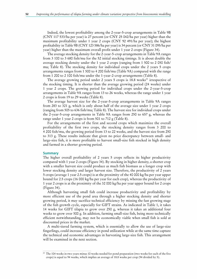
Improving the performance of tilapia farming under climate variation: perspective from bioeconomic modelling52
Indeed, the lowest profitability among the 2-year-5-crop arrangements in Table 9B (CNY 117 533/ha per year) is 27 percent (or CNY 25 042/ha per year) higher than the maximum profitability under 1 year 2 crops (CNY 92 491/ha per year); the highest profitability in Table 9B (CNY 123 586/ha per year) is 34 percent (or CNY 31 095/ha per year) higher than the maximum overall profit under 1 year 2 crops (Figure 34).
The average stocking density for the 2-year-5-crop arrangements in Table 9A ranges from 3 100 to 3 680 fish/mu for the 52 initial stocking timings. It is about double the average stocking density under the 1 year 2 crops (ranging from 1 500 to 2 050 fish/mu; Table 8). The stocking density for individual crops under the 2 years 5 crops arrangements ranges from 1 500 to 4 200 fish/mu (Table 9A) compared with the range from 1 200 to 2 100 fish/mu under the 1-year-2-crop arrangements (Table 8).
The average growing period under 2 years 5 crops is 18.8 weeks21 irrespective of the stocking timing. It is shorter than the average growing period (24 weeks) under 1 year 2 crops. The growing period for individual crops under the 2-year-5-crop arrangements in Table 9A ranges from 13 to 26 weeks, whereas the range under 1 year 2 crops is from 19 to 29 weeks (Table 8).
The average harvest size for the 2-year-5-crop arrangements in Table 9A ranges from 283 to 321 g, which is only about half of the average size under 1 year 2 crops (ranging from 505 to 636 fish/mu; Table 8). The harvest size for individual crops under the 2-year-5-crop arrangements in Table 9A ranges from 250 to 657 g, whereas the range under 1 year 2 crops is from 501 to 712 g (Table 8).
For the arrangements of the first and second crops which maximize the overall profitability of the first two crops, the stocking density ranges from 3 200 to 4 200 fish/mu, the growing period from 13 to 22 weeks, and the harvest size from 250 to 313 g. These results indicate that given no price discrepancy between small- and large-size fish, it is more profitable to harvest small-size fish stocked in high density and farmed in a shorter growing period.
SummaryThe higher overall profitability of 2 years 5 crops reflects its higher productivity compared with 1 year 2 crops (Figure 34). By stocking in higher density, a shorter crop with a smaller harvest size could produce as much fish biomass as a longer crop with lower stocking density and larger harvest size. Therefore, the productivity of 2 years 5 crops (average 1 year 2.5 crops) is at the proximity of the 40 000 kg/ha per year upper bound for 2.5 crops (16 000 kg/ha per year for each crop), whereas the productivity of 1 year 2 crops is at the proximity of the 32 000 kg/ha per year upper bound for 2 crops (Figure 34).
Although harvesting small fish could increase productivity and profitability by more efficient use of the pond area through a higher stocking density and shorter growing period, it may sacrifice technical efficiency by missing the fast growing stage of the fish growth cycle, especially for GIFT strains. As indicated in Table 1, it takes 14 weeks for GIFT tilapia to grow over 250 g, whereas it takes an additional four weeks to grow over 500 g. In addition, farming small-size fish, being more technically efficient notwithstanding, may not be economically viable when small fish is sold at discounted prices in the market.
A multi-tiered farming system, which is essentially to allow the use of large-size fingerlings, could increase efficiency in pond utilization while at the same time capture the technical and economic advantages in harvesting large-size fish. This arrangement will be examined in the next section.
21 The 104 weeks in two years minus 10 weeks needed for pond preparation (two weeks for each of the five crops) is equal to 94 weeks, which implies an average of 18.8 weeks per crop (94 divided by 5).

53Optimizing crop arrangements for better performance
4.4 MULTI-TIER FARMING SYSTEMSUnder the 1-year-2-crop arrangement where the targeted harvest size is above 500 g, the average stocking density (1 g fingerling) is mostly less than 2 000 fish/mu (Table 8). The stocking density cannot be made higher because doing so would result in the fish biomass exceeding the capacity limit at harvest. However, during the growing period when the fish are below the targeted harvest size, the fish biomass in the pond would be well under the capacity limit, which results in inefficient use of the pond area. Thus, stocking at a higher density for a smaller harvest size could increase productivity by utilizing the pond area more efficiently.
Another way to improve the efficiency in the utilization of the pond area is to adjust the stocking density according to fish size so as to maintain the fish biomass at high levels. For example, in Hainan province, in China, tilapia farmers often stock 3–4 cm fingerlings in nursery ponds at 5 000–10 000 fish/mu and grow them for 50–60 days until they reach 13–17 cm (100–150 g); they then stock the large-size fingerlings at 1 800–2 000 fish/mu in outgrowing ponds and raise them to the targeted harvest size. Such a two-tier farming system enhances the efficiency in utilizing pond areas. Some farmers even add an additional tier by nursing 1 cm fry into 3–4 cm fingerlings in ponds or hapas at 30 000–50 000 fish/mu density (Yang, 2015, p. 51).
In this section, the advanced bioeconomic model is used to examine the technical and economic performance of a two-tier tilapia farming system and compare it to the 1-year-2-crop benchmark. To simplify the model set-up, the production costs of large fingerlings of different size are estimated first and then the costs are used as the shadow prices of the fingerlings to estimate the profitability of farming arrangements that allow farmers to stock fingerlings of different sizes.
Production costs of large fingerlingsThe advanced bioeconomic model is used to estimate the production costs of large fingerlings (50 g, 100 g or 150 g). Based on the economic parameters specified in Table 3 and the technical parameters specified in Table 10, nearly 230 000 cases of fingerling nursing arrangements (52 different stocking timings, 218 different stocking density and 20 different nursing periods) are simulated in the advanced model.
TABLE 10Technical parameters used in the simulation of the production of large fingerlings
Parameters Specification
Initial fingerling size 1 g
Stocking timing 52 weekly stocking timings – see Table 8
Stocking density1 500–110 000 fish/mu with 500 fish/mu increments (e.g. 1 500 fish/mu, 2 000 fish/mu, 2 500 fish/mu, and so on)
Nursing period 1 to 20 weeks, which is enough time for 1 g fingerlings to grow up to 150 g in all seasons
Among them, the cases that produce 40–60 g fingerlings are used to estimate the production costs of 50 g fingerling. As the size of the fingerling harvested is usually not equal to 50 g exactly, the actual production cost of the fingerling would need to be normalized into a cost for a 50 g fingerling. For example, suppose in an arrangement the cost of producing 45 g fingerlings is CNY 0.36/fish, then the normalized cost for producing 50 g fingerlings under that arrangement would be CNY 0.4/fish (equal to CNY 0.36/fish ÷ 45 g × 50 g). For a harvest date, there may be different normalized production costs of 50 g fingerlings because more than one arrangement harvests fingerlings within the size range on that date. Under this situation, the lowest normalized cost is deemed the production cost of 50 g fingerlings for the harvest date. The range of 40–60 g is selected to ensure that for each of the 52 weekly harvest date

Improving the performance of tilapia farming under climate variation: perspective from bioeconomic modelling54
there is at least one arrangement that produces fingerlings at a size within the range – this may not be the case for a narrower range (e.g. 45–55 g).
The production costs of 100 g and 150 g fingerlings are estimated in a similar way.22 The results indicate that the production costs of 50 g, 100 g and 150 g fingerlings are at the range of CNY 0.34–0.39/fish (average CNY 0.36/fish), CNY 0.59–0.68/fish (average CNY 0.63/fish), and CNY 0.87–1.00/fish (average CNY 0.93/fish), respectively (Table 11; Figures 35 and 36).
The production costs of large fingerlings in terms of weight are CNY 7.10/kg, CNY 6.28/kg and CNY 6.20/kg for 50 g, 100 g and 150 g fingerlings, respectively (Figure 36). The costs are much lower than those shown in Figure 9, where the stocking density is 1 200 fish/mu. This indicates that nursing fingerlings in higher stocking density before stocking the large-size fingerlings in outgrowing ponds is more efficient than stocking small-size fingerlings directly in outgrowing ponds and growing them to harvest size.
Stocking large-size fingerlings – 1 year 3 cropsWhen large-sized fingerlings are used, it is possible to produce three crops within a year. The advanced model is used to simulate the arrangements of 1 year 3 crops and compare its technical and economic performance to the 1-year-2-crop arrangements.
The technical and economic parameters used in the simulation is mostly the same as those used in the 1-year-2-crop simulation. A key difference is that, as opposed to 1 g fingerlings being used in the 1-year-2-crop simulation, the farmer under the 1-year-3-crop set-up has options to use fingerlings of four different sizes (1 g, 50 g, 100 g or 150 g) at the costs specified in Table 11 and that in Table 3 for 1 g fingerlings.
The resulting 1-year-3-crop arrangements that maximize the overall profit for the 52 weekly stocking timings are presented in Tables 12A and 12B. The comparison between 1 year 3 crops and the other two crop arrangements is summarized in Table 13.
The results indicate that for all the 52 initial stocking timings, the profitability of 1 year 3 crops under the two-tier system would be substantially higher than that under the 1 year 2 crops (Figure 37).
• The average profitability across the 52 initial stocking timings is nearly CNY 150 000/ha per year, which is higher than that under 1 years 2 crops (Table 13).
• The average growing period under 1 year 3 crops is about 15 weeks, shorter than that under 1 year 2 crops (Table 13).
• The average stocking density under 1 year 3 crops is close to 1 900 fish/mu, which is slightly higher than that under 1 year 2 crops (Table 13).
• The average harvest size under 1 year 3 crops is 535 g, which is slightly smaller than that under 1 year 2 crops (Table 13).
• The average productivity under 1 year 3 crops is 45 000 kg/ha per year, which is higher than that under 1 year 2 crops (Table 13).
It seems that the higher profitability is primarily due to the higher productivity under 1 year 3 crops, where the use of large fingerlings shortens the growing period and hence allows an extra crop compared to 1 year 2 crops. It should be noted, however, that the use of large fingerlings per se may not improve profitability; it is the efficiency gain from nursing fingerlings at higher stocking density that leads to higher profitability.
The two-tier, 1-year-3-crop arrangement that gives the highest overall profitability is as follows (Table 14).23
22 The size range for estimating the cost of 100 g and 150 g fingerlings is 85–115 g and 135–165 g, respectively.
23 The sequence of the first, second and third crop is arbitrarily specified.

55Optimizing crop arrangements for better performance
TABLE 11Production of large-size fingerlings
Large-size fingerlings
harvested on:
50 g fingerlings 100 g fingerlings 150 g fingerlings
1 g fingerlings stocked on:
Stocking density
(fish/mu)
Nursing period
(weeks)
Normalized fingerling
production cost (CNY/fish)
1 g fingerlings stocked on:
Stocking density
(fish/mu)
Nursing period
(weeks)
Normalized fingerling
production cost (CNY/fish)
1 g fingerlings stocked on:
Stocking density
(fish/mu)
Nursing period
(weeks)
Normalized fingerling
production cost (CNY/fish)
01/01/year t 29/10/year t-1 11 000 9 0.35 15/10/year t-1 10 500 11 0.60 01/10/year t-1 6 500 13 0.88
08/01/year t 05/11/year t-1 11 000 9 0.39 15/10/year t-1 10 000 12 0.59 08/10/year t-1 7 500 13 0.87
15/01/year t 05/11/year t-1 11 000 10 0.37 22/10/year t-1 11 000 12 0.60 08/10/year t-1 7 000 14 0.88
22/01/year t 05/11/year t-1 11 000 11 0.37 22/10/year t-1 11 000 13 0.60 08/10/year t-1 6 500 15 0.89
29/01/year t 05/11/year t-1 11 000 12 0.35 22/10/year t-1 10 000 14 0.59 15/10/year t-1 7 500 15 0.88
05/02/year t 12/11/year t-1 11 000 12 0.38 29/10/year t-1 11 000 14 0.61 15/10/year t-1 6 500 16 0.90
12/02/year t 12/11/year t-1 11 000 13 0.36 29/10/year t-1 10 500 15 0.61 22/10/year t-1 4 500 16 1.00
19/02/year t 19/11/year t-1 11 000 13 0.39 29/10/year t-1 9 500 16 0.62 22/10/year t-1 7 500 17 0.91
26/02/year t 19/11/year t-1 11 000 14 0.37 05/11/year t-1 11 000 16 0.63 22/10/year t-1 6 500 18 0.92
05/03/year t 26/11/year t-1 11 000 14 0.38 05/11/year t-1 9 500 17 0.63 29/10/year t-1 7 000 18 0.94
12/03/year t 03/12/year t-1 11 000 14 0.38 12/11/year t-1 9 000 17 0.64 05/11/year t-1 7 000 18 0.95
19/03/year t 10/12/year t-1 11 000 14 0.37 19/11/year t-1 8 500 17 0.65 05/11/year t-1 6 500 19 0.94
26/03/year t 24/12/year t-1 11 000 13 0.36 26/11/year t-1 10 000 17 0.65 12/11/year t-1 7 000 19 0.95
02/04/year t 08/01/year t 11 000 12 0.36 03/12/year t-1 9 500 17 0.68 19/11/year t-1 7 000 19 0.98
09/04/year t 05/02/year t 10 000 9 0.36 10/12/year t-1 8 000 17 0.68 26/11/year t-1 6 500 19 1.00
16/04/year t 19/02/year t 9 500 8 0.35 22/01/year t 7 000 12 0.66 17/12/year t-1 5 500 17 1.00
23/04/year t 05/03/year t 9 000 7 0.35 29/01/year t 6 000 12 0.65 15/01/year t 4 500 14 0.99
30/04/year t 12/03/year t 10 500 7 0.34 26/02/year t 5 500 9 0.64 05/02/year t 4 500 12 0.96
07/05/year t 26/03/year t 8 500 6 0.34 05/03/year t 5 500 9 0.62 26/02/year t 4 500 10 0.93
14/05/year t 02/04/year t 8 500 6 0.35 12/03/year t 5 500 9 0.63 05/03/year t 4 500 10 0.93
21/05/year t 09/04/year t 10 000 6 0.35 19/03/year t 5 500 9 0.63 12/03/year t 4 500 10 0.94
28/05/year t 09/04/year t 10 500 7 0.34 26/03/year t 5 500 9 0.62 19/03/year t 4 500 10 0.93
04/06/year t 16/04/year t 9 000 7 0.35 02/04/year t 5 500 9 0.63 26/03/year t 4 500 10 0.93
11/06/year t 23/04/year t 10 500 7 0.36 09/04/year t 6 000 9 0.63 26/03/year t 4 000 11 0.93
18/06/year t 30/04/year t 10 000 7 0.37 09/04/year t 6 500 10 0.64 02/04/year t 4 500 11 0.94
25/06/year t 30/04/year t 9 000 8 0.35 16/04/year t 5 500 10 0.64 09/04/year t 4 000 11 0.94
02/07/year t 07/05/year t 9 000 8 0.35 23/04/year t 6 000 10 0.64 16/04/year t 4 500 11 0.95
09/07/year t 14/05/year t 9 500 8 0.36 30/04/year t 6 000 10 0.65 16/04/year t 4 000 12 0.95
16/07/year t 21/05/year t 9 500 8 0.36 30/04/year t 6 000 11 0.65 23/04/year t 4 000 12 0.95
23/07/year t 28/05/year t 9 500 8 0.35 07/05/year t 5 500 11 0.64 30/04/year t 4 500 12 0.95
30/07/year t 04/06/year t 9 500 8 0.35 14/05/year t 5 500 11 0.65 07/05/year t 4 500 12 0.96
06/08/year t 11/06/year t 9 000 8 0.35 21/05/year t 5 500 11 0.64 14/05/year t 4 500 12 0.96
13/08/year t 18/06/year t 8 000 8 0.35 28/05/year t 5 500 11 0.64 21/05/year t 4 500 12 0.96
20/08/year t 25/06/year t 9 000 8 0.35 04/06/year t 6 000 11 0.65 28/05/year t 4 500 12 0.96
27/08/year t 02/07/year t 10 000 8 0.35 11/06/year t 6 500 11 0.65 04/06/year t 4 500 12 0.95
03/09/year t 16/07/year t 9 000 7 0.36 25/06/year t 5 500 10 0.64 11/06/year t 4 500 12 0.95
10/09/year t 23/07/year t 9 500 7 0.35 02/07/year t 5 000 10 0.64 25/06/year t 4 500 11 0.95
17/09/year t 30/07/year t 8 500 7 0.35 16/07/year t 5 500 9 0.64 02/07/year t 4 500 11 0.94
24/09/year t 06/08/year t 10 000 7 0.34 23/07/year t 5 500 9 0.64 09/07/year t 4 000 11 0.94
01/10/year t 20/08/year t 8 500 6 0.35 30/07/year t 5 500 9 0.63 16/07/year t 4 500 11 0.94
08/10/year t 27/08/year t 8 500 6 0.34 06/08/year t 5 500 9 0.62 30/07/year t 4 500 10 0.93
15/10/year t 03/09/year t 9 500 6 0.34 20/08/year t 5 500 8 0.61 06/08/year t 4 500 10 0.91
22/10/year t 10/09/year t 10 000 6 0.34 27/08/year t 6 000 8 0.61 13/08/year t 4 500 10 0.90
29/10/year t 17/09/year t 9 500 6 0.34 03/09/year t 6 000 8 0.62 20/08/year t 4 500 10 0.90
05/11/year t 24/09/year t 9 500 6 0.34 10/09/year t 6 500 8 0.62 27/08/year t 4 500 10 0.90
12/11/year t 01/10/year t 10 000 6 0.35 17/09/year t 6 000 8 0.61 03/09/year t 4 500 10 0.90
19/11/year t 08/10/year t 11 000 6 0.35 17/09/year t 7 500 9 0.61 10/09/year t 5 000 10 0.89
26/11/year t 15/10/year t 11 000 6 0.36 24/09/year t 7 000 9 0.60 17/09/year t 5 500 10 0.89
03/12/year t 22/10/year t 11 000 6 0.36 01/10/year t 6 500 9 0.60 24/09/year t 5 500 10 0.89
10/12/year t 22/10/year t 11 000 7 0.34 01/10/year t 9 000 10 0.60 24/09/year t 6 000 11 0.88
17/12/year t 29/10/year t 11 000 7 0.37 08/10/year t 8 000 10 0.60 01/10/year t 7 000 11 0.88
24/12/year t 29/10/year t 11 000 8 0.36 08/10/year t 8 500 11 0.59 01/10/year t 7 500 12 0.88

Improving the performance of tilapia farming under climate variation: perspective from bioeconomic modelling56
TABLE 12A1-year-3-crop arrangements that maximize the overall profit for each of the 52 initial stocking timings
Stocking timingStocking size
(g)Stocking density
(fish/mu)Growing period
(weeks)Harvest size
(g)
1st crop 2nd crop 3rd crop1st
crop2nd crop
3rd crop
Average1st
crop2nd crop
3rd crop
Average1st
crop2nd crop
3rd crop
Average1st
crop2nd crop
3rd crop
Average
01/01/1st year 23/04/1st year 01/10/1st year 150 1 100 86 2 000 1 800 1 900 1 900 14 21 11 15.33 530 510 554 532
08/01/1st year 23/04/1st year 01/10/1st year 150 1 100 87 2 100 1 800 1 800 1 900 13 21 12 15.33 502 510 583 530
15/01/1st year 30/04/1st year 08/10/1st year 150 1 100 86 2 000 1 800 1 900 1 900 13 21 12 15.33 531 511 539 528
22/01/1st year 30/04/1st year 15/10/1st year 150 1 100 83 2 000 2 100 2 100 2 067 12 22 12 15.33 523 504 506 511
29/01/1st year 21/05/1st year 29/10/1st year 100 1 150 83 1 900 2 100 2 100 2 033 14 21 11 15.33 551 502 502 517
05/02/1st year 21/05/1st year 29/10/1st year 100 1 150 82 2 000 2 100 2 000 2 033 13 21 12 15.33 519 502 518 513
12/02/1st year 21/05/1st year 29/10/1st year 100 1 150 81 2 000 2 100 1 900 2 000 12 21 13 15.33 505 502 548 517
19/02/1st year 21/05/1st year 29/10/1st year 100 1 150 80 1 900 2 100 1 800 1 933 11 21 14 15.33 506 502 587 530
26/02/1st year 21/05/1st year 29/10/1st year 150 1 150 95 1 900 2 100 1 700 1 900 10 21 15 15.33 549 502 611 550
05/03/1st year 21/05/1st year 05/11/1st year 150 1 150 103 2 000 1 800 1 900 1 900 9 22 15 15.33 509 580 559 548
12/03/1st year 21/05/1st year 05/11/1st year 150 1 150 100 1 800 1 800 1 800 1 800 8 22 16 15.33 504 580 592 559
19/03/1st year 28/05/1st year 05/11/1st year 150 1 100 80 1 700 2 000 2 000 1 900 8 21 17 15.33 512 529 522 521
26/03/1st year 06/08/1st year 19/11/1st year 50 50 150 89 1 100 1 900 1 900 1 633 17 13 16 15.33 730 549 559 593
02/04/1st year 16/07/1st year 29/10/1st year 50 50 50 50 1 500 2 000 2 000 1 833 13 13 20 15.33 514 505 533 518
09/04/1st year 20/08/1st year 03/12/1st year 50 50 150 90 1 200 1 800 2 000 1 667 17 13 16 15.33 689 592 530 590
16/04/1st year 17/09/1st year 24/12/1st year 1 50 150 73 1 600 2 100 2 100 1 933 20 12 14 15.33 500 507 500 503
23/04/1st year 01/10/1st year 08/01/2nd year 1 100 150 87 1 800 1 800 2 100 1 900 21 12 13 15.33 510 583 502 530
30/04/1st year 15/10/1st year 22/01/2nd year 1 100 150 83 2 100 2 100 2 000 2 067 22 12 12 15.33 504 506 523 511
07/05/1st year 29/10/1st year 29/01/2nd year 1 150 150 104 1 800 2 100 1 900 1 933 23 11 12 15.33 589 502 546 543
14/05/1st year 29/10/1st year 29/01/2nd year 1 150 100 86 1 900 2 100 2 000 2 000 22 11 13 15.33 549 502 502 517
21/05/1st year 29/10/1st year 29/01/2nd year 1 150 100 83 2 100 2 100 1 900 2 033 21 11 14 15.33 502 502 551 517
28/05/1st year 05/11/1st year 19/02/2nd year 1 150 100 84 2 000 2 000 2 100 2 033 21 13 12 15.33 529 518 502 516
04/06/1st year 05/11/1st year 05/03/2nd year 1 150 100 82 2 000 1 900 1 800 1 900 20 15 11 15.33 509 559 508 525
11/06/1st year 12/11/1st year 12/03/2nd year 1 150 100 81 2 100 2 000 1 600 1 900 20 15 11 15.33 506 523 529 519
18/06/1st year 19/11/1st year 26/03/2nd year 1 150 100 81 2 000 1 900 1 500 1 800 20 16 10 15.33 530 559 512 535
25/06/1st year 19/11/1st year 26/03/2nd year 1 150 100 81 2 000 1 900 1 600 1 833 19 16 11 15.33 505 559 528 530
02/07/1st year 03/12/1st year 09/04/2nd year 1 150 100 85 1 800 2 000 1 500 1 767 20 16 10 15.33 583 530 502 540
09/07/1st year 03/12/1st year 09/04/2nd year 1 150 100 82 2 000 2 000 1 500 1 833 19 16 11 15.33 530 530 528 529
16/07/1st year 24/12/1st year 16/04/2nd year 1 150 100 90 1 600 2 100 1 600 1 767 21 14 11 15.33 659 500 504 549
23/07/1st year 24/12/1st year 16/04/2nd year 1 150 100 88 1 700 2 100 1 500 1 767 20 14 12 15.33 610 500 542 547
30/07/1st year 24/12/1st year 16/04/2nd year 1 150 50 72 1 900 2 100 1 400 1 800 19 14 13 15.33 549 500 509 520
06/08/1st year 08/01/2nd year 23/04/2nd year 1 150 100 85 1 900 2 100 1 400 1 800 20 13 13 15.33 559 502 587 544
13/08/1st year 08/01/2nd year 23/04/2nd year 1 150 50 70 2 000 2 100 1 600 1 900 19 13 14 15.33 517 502 510 509
20/08/1st year 22/01/2nd year 30/04/2nd year 1 150 50 69 2 000 2 000 1 500 1 833 20 12 14 15.33 522 523 514 520
27/08/1st year 03/12/1st year 09/04/2nd year 50 150 50 89 2 000 2 000 1 100 1 700 12 16 18 15.33 528 530 736 574
03/09/1st year 24/12/1st year 16/04/2nd year 50 150 50 94 1 600 2 100 1 100 1 600 14 14 18 15.33 648 500 726 601
10/09/1st year 01/01/2nd year 23/04/2nd year 50 150 50 91 1 700 2 000 1 200 1 633 14 14 18 15.33 618 530 700 602
17/09/1st year 24/12/1st year 16/04/2nd year 50 150 1 73 2 100 2 100 1 600 1 933 12 14 20 15.33 507 500 500 503
24/09/1st year 08/01/2nd year 23/04/2nd year 50 150 1 74 2 100 2 100 1 500 1 900 13 13 20 15.33 506 502 512 506
01/10/1st year 08/01/2nd year 23/04/2nd year 100 150 1 87 1 800 2 100 1 800 1 900 12 13 21 15.33 583 502 510 530
08/10/1st year 08/01/2nd year 23/04/2nd year 100 150 1 86 2 000 2 100 1 900 2 000 11 13 22 15.33 515 502 530 515
15/10/1st year 22/01/2nd year 30/04/2nd year 100 150 1 83 2 100 2 000 2 100 2 067 12 12 22 15.33 506 523 504 511
22/10/1st year 22/01/2nd year 30/04/2nd year 150 150 1 103 1 900 2 000 1 800 1 900 11 12 23 15.33 550 523 581 550
29/10/1st year 29/01/2nd year 21/05/2nd year 150 100 1 83 2 100 1 900 2 100 2 033 11 14 21 15.33 502 551 502 517
05/11/1st year 19/02/2nd year 21/05/2nd year 150 100 1 86 2 000 1 900 1 800 1 900 13 11 22 15.33 518 506 580 534
12/11/1st year 12/03/2nd year 21/05/2nd year 150 150 1 106 2 000 1 800 1 600 1 800 15 8 23 15.33 523 504 653 555
19/11/1st year 09/04/2nd year 13/08/2nd year 100 50 50 68 1 900 1 300 2 100 1 767 18 16 12 15.33 544 640 500 550
26/11/1st year 09/04/2nd year 13/08/2nd year 150 50 50 87 1 800 1 300 1 800 1 633 17 16 13 15.33 591 640 578 599
03/12/1st year 09/04/2nd year 20/08/2nd year 150 50 50 90 2 000 1 200 1 800 1 667 16 17 13 15.33 530 689 592 590
10/12/1st year 09/04/2nd year 17/09/2nd year 150 1 100 88 2 000 1 700 2 000 1 900 15 21 10 15.33 504 520 531 518
17/12/1st year 16/04/2nd year 24/09/2nd year 150 1 100 87 2 000 1 800 2 000 1 933 15 21 10 15.33 521 508 529 520
24/12/1st year 16/04/2nd year 17/09/2nd year 150 1 50 73 2 100 1 600 2 100 1 933 14 20 12 15.33 500 500 507 503

57Optimizing crop arrangements for better performance
TABLE 12BProductivity and profitability for the 1-year-3-crop arrangements in Table 12A
Stocking timing
Productivity Profitability
Weekly (kg/ha/week) Annual
(kg/ha/year)
Weekly (CNY/ha/week) Annual
(CNY/ha/year) 1st crop 2nd crop 3rd crop 1st crop 2nd crop 3rd crop Overall 1st crop 2nd crop 3rd crop Overall
01/01/1st year 23/04/1st year 01/10/1st year 994 598 1 216 874 45 462 3 281 1 712 4 708 2 943 153 060
08/01/1st year 23/04/1st year 01/10/1st year 1 054 598 1 124 871 45 296 3 519 1 712 4 361 2 946 153 207
15/01/1st year 30/04/1st year 08/10/1st year 1 063 600 1 098 868 45 118 3 393 1 732 4 314 2 906 151 120
22/01/1st year 30/04/1st year 15/10/1st year 1 121 662 1 137 914 47 507 3 628 1 646 4 535 2 958 153 802
29/01/1st year 21/05/1st year 29/10/1st year 981 687 1 215 910 47 309 2 929 1 961 4 705 2 945 153 130
05/02/1st year 21/05/1st year 29/10/1st year 1 039 687 1 109 902 46 922 3 136 1 961 4 257 2 918 151 732
12/02/1st year 21/05/1st year 29/10/1st year 1 081 687 1 042 896 46 570 3 362 1 961 3 989 2 923 151 993
19/02/1st year 21/05/1st year 29/10/1st year 1 110 687 990 886 46 077 3 618 1 961 3 770 2 932 152 452
26/02/1st year 21/05/1st year 29/10/1st year 1 303 687 916 904 47 022 3 861 1 961 3 387 2 866 149 013
05/03/1st year 21/05/1st year 05/11/1st year 1 388 652 937 901 46 868 4 169 1 873 3 468 2 880 149 771
12/03/1st year 21/05/1st year 05/11/1st year 1 360 652 888 870 45 245 4 453 1 873 3 257 2 848 148 120
19/03/1st year 28/05/1st year 05/11/1st year 1 304 690 825 857 44 578 4 219 2 017 3 004 2 801 145 666
26/03/1st year 06/08/1st year 19/11/1st year 634 1 042 885 839 43 607 1 864 3 529 3 152 2 790 145 097
02/04/1st year 16/07/1st year 29/10/1st year 771 1 010 726 821 42 706 2 566 3 235 2 646 2 793 145 231
09/04/1st year 20/08/1st year 03/12/1st year 653 1 065 883 851 44 270 1 888 3 806 3 090 2 857 148 583
16/04/1st year 17/09/1st year 24/12/1st year 546 1 141 985 841 43 738 1 678 4 430 3 323 2 925 152 110
23/04/1st year 01/10/1st year 08/01/2nd year 598 1 124 1 054 871 45 296 1 712 4 361 3 519 2 946 153 207
30/04/1st year 15/10/1st year 22/01/2nd year 662 1 137 1 121 914 47 507 1 646 4 535 3 628 2 958 153 802
07/05/1st year 29/10/1st year 29/01/2nd year 637 1 215 1 111 909 47 269 1 677 4 705 3 415 2 902 150 898
14/05/1st year 29/10/1st year 29/01/2nd year 652 1 215 1 005 895 46 521 1 809 4 705 3 118 2 911 151 349
21/05/1st year 29/10/1st year 29/01/2nd year 687 1 215 981 910 47 309 1 961 4 705 2 929 2 945 153 130
28/05/1st year 05/11/1st year 19/02/2nd year 690 1 036 1 129 908 47 218 2 017 3 950 3 182 2 888 150 186
04/06/1st year 05/11/1st year 05/03/2nd year 694 937 1 055 864 44 926 2 132 3 468 3 175 2 830 147 138
11/06/1st year 12/11/1st year 12/03/2nd year 725 923 977 853 44 343 2 215 3 377 3 007 2 793 145 220
18/06/1st year 19/11/1st year 26/03/2nd year 723 885 960 834 43 358 2 268 3 152 3 147 2 777 144 409
25/06/1st year 19/11/1st year 26/03/2nd year 722 885 974 841 43 748 2 378 3 152 2 927 2 783 144 722
02/07/1st year 03/12/1st year 09/04/2nd year 716 883 942 826 42 944 2 410 3 090 3 123 2 810 146 115
09/07/1st year 03/12/1st year 09/04/2nd year 757 883 914 840 43 681 2 594 3 090 2 871 2 835 147 430
16/07/1st year 24/12/1st year 16/04/2nd year 688 985 930 840 43 670 2 391 3 323 2 897 2 804 145 814
23/07/1st year 24/12/1st year 16/04/2nd year 706 985 871 837 43 506 2 555 3 323 2 624 2 810 146 105
30/07/1st year 24/12/1st year 16/04/2nd year 746 985 713 810 42 116 2 759 3 323 2 478 2 851 148 268
06/08/1st year 08/01/2nd year 23/04/2nd year 724 1 054 822 847 44 065 2 754 3 519 2 495 2 900 150 807
13/08/1st year 08/01/2nd year 23/04/2nd year 738 1 054 765 837 43 549 2 871 3 519 2 474 2 936 152 668
20/08/1st year 22/01/2nd year 30/04/2nd year 712 1 121 722 825 42 907 2 790 3 628 2 411 2 899 150 742
27/08/1st year 03/12/1st year 09/04/2nd year 1 132 883 607 844 43 885 4 121 3 090 1 687 2 828 147 069
03/09/1st year 24/12/1st year 16/04/2nd year 972 985 599 833 43 303 3 642 3 323 1 704 2 799 145 526
10/09/1st year 01/01/2nd year 23/04/2nd year 985 994 630 851 44 245 3 808 3 281 1 759 2 857 148 586
17/09/1st year 24/12/1st year 16/04/2nd year 1 141 985 546 841 43 738 4 430 3 323 1 678 2 925 152 110
24/09/1st year 08/01/2nd year 23/04/2nd year 1 063 1 054 523 832 43 266 4 285 3 519 1 642 2 946 153 196
01/10/1st year 08/01/2nd year 23/04/2nd year 1 124 1 054 598 871 45 296 4 361 3 519 1 712 2 946 153 207
08/10/1st year 08/01/2nd year 23/04/2nd year 1 188 1 054 629 891 46 341 4 674 3 519 1 637 2 939 152 839
15/10/1st year 22/01/2nd year 30/04/2nd year 1 137 1 121 662 914 47 507 4 535 3 628 1 646 2 958 153 802
22/10/1st year 22/01/2nd year 30/04/2nd year 1 206 1 121 628 905 47 064 4 681 3 628 1 569 2 901 150 868
29/10/1st year 29/01/2nd year 21/05/2nd year 1 215 981 687 910 47 309 4 705 2 929 1 961 2 945 153 130
05/11/1st year 19/02/2nd year 21/05/2nd year 1 036 1 110 652 877 45 627 3 950 3 618 1 873 2 908 151 240
12/11/1st year 12/03/2nd year 21/05/2nd year 923 1 360 627 865 44 971 3 377 4 453 1 781 2 817 146 471
19/11/1st year 09/04/2nd year 13/08/2nd year 775 693 1 126 841 43 729 2 770 2 081 3 845 2 821 146 691
26/11/1st year 09/04/2nd year 13/08/2nd year 840 693 1 040 847 44 037 2 943 2 081 3 588 2 831 147 189
03/12/1st year 09/04/2nd year 20/08/2nd year 883 653 1 065 851 44 270 3 090 1 888 3 806 2 857 148 583
10/12/1st year 09/04/2nd year 17/09/2nd year 889 577 1 327 852 44 312 3 149 1 630 4 711 2 837 147 544
17/12/1st year 16/04/2nd year 24/09/2nd year 919 597 1 323 870 45 232 3 073 1 677 4 798 2 854 148 387
24/12/1st year 16/04/2nd year 17/09/2nd year 985 546 1 141 841 43 738 3 323 1 678 4 430 2 925 152 110

Improving the performance of tilapia farming under climate variation: perspective from bioeconomic modelling58
• First crop: stocking 1 g fingerlings, 2 100 fish/mu on 30 April and harvesting 504 g fish after 22 weeks, on 1 October, for 662 kg/ha per week and CNY 1 645/ha per week.
• Second crop: stocking 100 g fingerlings, 2 100 fish/mu on 15 October and harvesting 506 g fish after 12 weeks, on 8 January the next year, for 1 137 kg/ha per week and CNY 4 535/ha per week.
• Third crop: stocking 150 g fingerlings, 2 000 fish/mu on 22 January the next year and harvesting 523 g fish after 12 weeks, on 16 April the next year, for 1 121 kg/ha per week and CNY 3 628/ha per week.
• The overall productivity is 914 kg/ha per week (or 47 507 kg/ha per year).• The overall profitability is CNY 2 958/ha per week (or CNY 153 802/ha per year),
which is 66 percent higher than the maximum profitability under 1 year 2 crops. The fingerling costs in Table 11 only account for the costs of fingerling production.24
When the farmer purchases large-size fingerlings from commercial nurseries, the costs
24 The production cost includes the cost of harvesting large-size fingerlings from nursery ponds.
50 g (production cost)
100 g (production cost)
150 g (production cost)
1 g (purchase cost)
0
0.1
0.2
0.3
0.4
0.5
0.6
0.7
0.8
0.9
1
1.1
01/0
1/1s
t yea
r08
/01/
1st y
ear
15/0
1/1s
t yea
r22
/01/
1st y
ear
29/0
1/1s
t yea
r05
/02/
1st y
ear
12/0
2/1s
t yea
r19
/02/
1st y
ear
26/0
2/1s
t yea
r05
/03/
1st y
ear
12/0
3/1s
t yea
r19
/03/
1st y
ear
26/0
3/1s
t yea
r02
/04/
1st y
ear
09/0
4/1s
t yea
r16
/04/
1st y
ear
23/0
4/1s
t yea
r30
/04/
1st y
ear
07/0
5/1s
t yea
r14
/05/
1st y
ear
21/0
5/1s
t yea
r28
/05/
1st y
ear
04/0
6/1s
t yea
r11
/06/
1st y
ear
18/0
6/1s
t yea
r25
/06/
1st y
ear
02/0
7/1s
t yea
r09
/07/
1st y
ear
16/0
7/1s
t yea
r23
/07/
1st y
ear
30/0
7/1s
t yea
r06
/08/
1st y
ear
13/0
8/1s
t yea
r20
/08/
1st y
ear
27/0
8/1s
t yea
r03
/09/
1st y
ear
10/0
9/1s
t yea
r17
/09/
1st y
ear
24/0
9/1s
t yea
r01
/10/
1st y
ear
08/1
0/1s
t yea
r15
/10/
1st y
ear
22/1
0/1s
t yea
r29
/10/
1st y
ear
05/1
1/1s
t yea
r12
/11/
1st y
ear
19/1
1/1s
t yea
r26
/11/
1st y
ear
03/1
2/1s
t yea
r10
/12/
1st y
ear
17/1
2/1s
t yea
r24
/12/
1st y
ear
Cost
(CNY
/fish
)
Fingerling harvest date
FIGURE 35Costs of fingerlings of different sizes
7.10
6.28 6.20
0.360.63
0.93
50g 100g 150gCNY/kg CNY/fish
FIGURE 36Average production cost of large fingerlings*
* Average production costs for the 52 harvest dates in Table 11.
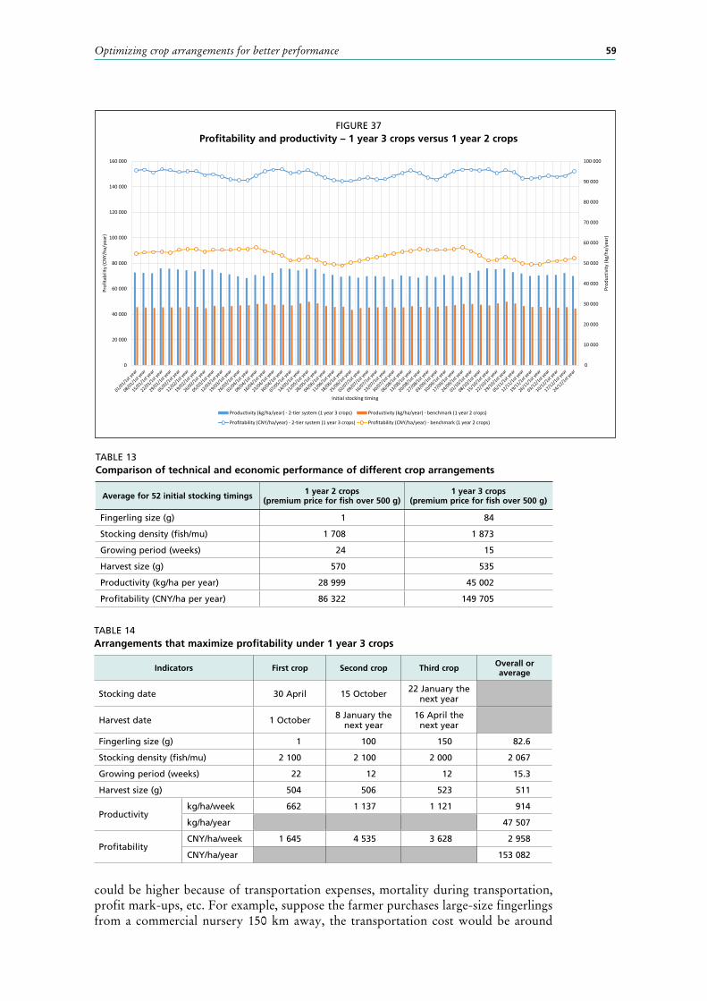
59Optimizing crop arrangements for better performance
could be higher because of transportation expenses, mortality during transportation, profit mark-ups, etc. For example, suppose the farmer purchases large-size fingerlings from a commercial nursery 150 km away, the transportation cost would be around
0
10 000
20 000
30 000
40 000
50 000
60 000
70 000
80 000
90 000
100 000
0
20 000
40 000
60 000
80 000
100 000
120 000
140 000
160 000
Prod
uctiv
ity (k
g/ha
/yea
r)
Prof
itabi
lity
(CNY
/ha/
year
)
Initial stocking timing
Productivity (kg/ha/year) - 2-tier system (1 year 3 crops) Productivity (kg/ha/year) - benchmark (1 year 2 crops)
Profitability (CNY/ha/year) - 2-tier system (1 year 3 crops) Profitability (CNY/ha/year) - benchmark (1 year 2 crops)
FIGURE 37Profitability and productivity – 1 year 3 crops versus 1 year 2 crops
TABLE 13Comparison of technical and economic performance of different crop arrangements
Average for 52 initial stocking timings 1 year 2 crops(premium price for fish over 500 g)
1 year 3 crops(premium price for fish over 500 g)
Fingerling size (g) 1 84
Stocking density (fish/mu) 1 708 1 873
Growing period (weeks) 24 15
Harvest size (g) 570 535
Productivity (kg/ha per year) 28 999 45 002
Profitability (CNY/ha per year) 86 322 149 705
TABLE 14Arrangements that maximize profitability under 1 year 3 crops
Indicators First crop Second crop Third crop Overall or average
Stocking date 30 April 15 October 22 January the next year
Harvest date 1 October 8 January the next year
16 April the next year
Fingerling size (g) 1 100 150 82.6
Stocking density (fish/mu) 2 100 2 100 2 000 2 067
Growing period (weeks) 22 12 12 15.3
Harvest size (g) 504 506 523 511
Productivitykg/ha/week 662 1 137 1 121 914
kg/ha/year 47 507
ProfitabilityCNY/ha/week 1 645 4 535 3 628 2 958
CNY/ha/year 153 082
Improving the performance of tilapia farming under climate variation: perspective from bioeconomic modelling60
CNY 1.25/kg, which amounts to 20 percent for the production cost of 100 g and 150 g fingerlings.25 Also suppose the commercial nursery requires 30 percent of profit margin, then the prices of the fingerlings would be 50 percent higher than the production costs in Table 11. Under this situation, the maximum overall profitability in Table 14 would be reduced from CNY 153 802/ha per year to CNY 130 857/ha per year. The reduced profitability would still be greater than that under 1 year 2 crops.
Summary A multi-tier farming system uses nursing ponds to raise fingerlings to large size before stocking them in outgrowing ponds. Such a system could increase efficiency in pond utilization through high stocking density in nursing ponds. The simulation results in the advanced model indicate that a two-tier farming system could increase overall profitability by 59 to 87 percent (depending on different initial stocking timings) compared with the baseline 1-year-2-crop arrangement of stocking 1 g fingerlings in outgrowing ponds.
25 A truck loaded with six oxygenated tanks for transporting live fish would cost CNY 7.5/km and CNY 1 125 for 150 km. The six tanks can hold 900 kg of live fish (150 kg each), which means the transportation cost is CNY 1.25/kg. Thus, the transportation costs for 100 g and 150 g fingerlings are CNY 0.125/fish and CNY 0.1875/fish, respectively. The costs are equal to around 20 percent of the production costs of the fingerlings (Figure 35).

61
5. Discussion
The technical performance of an aquaculture operation is measured by productivity, whereas the economic performance is measured by profitability. While the two are often positively correlated, farming practices and arrangements that increase productivity may not improve profitability. Therefore, farmers as well as researchers who exert constant effort to increase the yield would need to assess whether improved productivity would lead to higher profits.
Time matters. Profit (per ha) per crop is not a proper measure for comparing the profitability of crops with different growing periods; profit per unit of time (week, month or year) would be more accurate. However, it should be noted that for a crop with a length not equal to an integer number of years, profit per year is only a normalized measure of the profitability of the specific crop, but may not be a proper measure of the profitability of the operation. For example, given 1 g fingerlings and 1 200 fish/mu stocking density in the advanced model, the best single-crop profitability is CNY 1 921/ha per week, which amounts to CNY 99 879/ha per year. Yet the maximum profit of 1 year 2 crops is only CNY 92 491/ha per year because the CNY 1 921/ha per week crop occurring in the most favourable weather cannot repeat itself over time due to climate variation. Planning for an aquaculture operation should be based on arrangements that can be repeated over time, which could be multiple-crop arrangements (e.g. 1 year 2 crops, 2 years 5 crops, 1 year 3 crops, and so on).
Farming performance is jointly affected by stocking timing, fingerling size, stocking density and growing period. People often judge farming performance by how fast fish grow. Yet fish growth per se is not a good measure of technical or economic performance. Indeed, the simulation results of the advanced model indicate that given the same growing period, higher stocking density with slower fish growth often results in a higher yield than lower stocking density with faster fish growth.
Farmers as well as researchers are often interested in identifying the optimal stocking density, growing period and/or harvest size. Yet the simulation results of the advanced model indicate that under seasonal climate variation, arrangements that maximize the profitability of individual crops may not be optimal for overall profitability. Even the combination of two crops with their maximum profitability achieved may not be the optimal arrangement that maximizes the overall profitability of 1 year 2 crops – sacrificing the profitability in the first crop may render the second crop a more conducive stocking timing, and the resulting profitability gain in the second crop could outweigh the profit loss in the first crop.
The conjecture that harvesting small-size fish could be more profitable is confirmed by the simulation results – given no price discrepancy between small- and large-size fish, 2-year-5-crop arrangements with higher stocking density, a shorter growing period and smaller harvest size (around 300 g) tend to be more productive and profitable than 1-year-2-crop arrangements that harvest fish over 500 g.
The simulation results also indicate that by separating nursing and outgrowing, the two-tier farming system, which has become increasingly popular in China as well as other countries, could allow 1-year-3-crop arrangements that are more productive and profitable than the benchmark 1-year-2-crop arrangements.
It should be noted that none of the smaller harvest size, more crops or higher productivity is a sufficient condition for higher profits. Increasing stocking density and harvesting smaller fish could increase productivity but reduce profitability because the efficiency gain from having more fish biomass is outweighed by the efficiency loss

Improving the performance of tilapia farming under climate variation: perspective from bioeconomic modelling62
from missing the fast-growing part of the fish’s life cycle. Without the efficiency gain in the nursing stage through using the pond’s carrying capacity more completely with higher stocking density, stocking large-size fingerlings could allow 1 year 3 crops and increase productivity accordingly, but the profitability would not be improved.
Under seasonal variation in the water temperature, a 1-year-2-crop arrangement starting at the best initial stocking timing can be nearly 20 percent more profitable than the one starting at the worse initial stocking timing, even though both arrangements are subject to the same overall weather conditions. The profitability under 2 years 5 crops could be more than 30 percent higher than the maximum profitability under 1 year 2 crops. The profitability under 1 year 3 crops could be nearly 70 percent higher than the maximum profitability under 1 year 2 crops. These results indicate that there is a great potential to improve performance through optimized business and operational planning in farming arrangements.
Farmers may be able to optimize farming arrangements gradually based on experiences accumulated over years. But experience-based business and operational planning tends to be inaccurate and less flexible in adapting to changes in environmental, technical or economic conditions. Bioeconomic models can offer help. As the optimal arrangements of the individual crops that maximize the overall profitability of a multiple-crop cycle, be it 1-year-2-crop, 2-year-5-crop or 1-year-3-crop, tend to vary in stocking density, growing period and harvest size, tailor-made bioeconomic models need to be constructed based on specific farming conditions in order to provide guidance to farmers’ business and operational planning.
The bioeconomic model developed in this paper illustrates the methodology of constructing bioeconomic models for facilitating business and operational planning and shows the potential of optimal business and operational planning in improving farming performance. The model would need to be improved in many aspects in order to be more adequate for providing practical guidance to business and operational planning in the real world. Key areas for improvement include: (i) more rigorous modelling of fish growth based on more detailed, comprehensive data on tilapia growth under different conditions (water temperature, stocking density, feeding regimes, etc.); (ii) accounting for more environmental factors (water supply, climate changes, etc.); (iii) accounting for the seasonality of the availability and prices of seed, feed and other inputs as well as the fish price; (iv) accounting for the impact of water temperature on FCR; (v) allowing the farmer to adjust feeding practices according to different farming conditions; and (vi) introducing uncertainties to facilitate risk analysis.
It would take long-term, collective efforts of farmers, researchers, extension personnel and policymakers to realize the potential of bioeconomic modelling for better business and operational planning in aquaculture. The research community needs to provide more scientific data and information on tilapia growth under different farming conditions and direct more efforts towards building practical bioeconomic models for guiding business and operational planning in aquaculture. Fish farmers should embrace bioeconomic modelling as a scientific tool to help them actively seek improvement in the farming performance rather than forced to change only when the operation is losing money. The extension community should help researchers develop more practical models according to farmers’ needs and facilitate farmers’ use of bioeconomic modelling techniques and results in business and operational planning. Policymakers should recognize bioeconomic modelling as a knowledge-based, climate-smart innovation for improving farming performance and provide funding and coordination support to facilitate the enterprise.
63
References
Arnason, R. 1992. Optimal feeding schedules and harvesting time in aquaculture. Marine Resource Economics, 7: 15–35.
Bjørndal, T. 1988. Optimal harvest of farmed fish. Marine Resource Economics, 5: 139–159.Domínguez-May, R., Hernández, J.M., Gasca-Leyva, E. & Poot-López, G.R. 2011.
Effect of ration and size heterogeneity on harvest time: tilapia culture in Yucatan, Mexico. Aquaculture Economics & Management, 15(4): 278–301.
Engle, C. & Neira, I. 2005. Tilapia farm business management and economics: a training manual. Aquaculture Collaborative Research Support Program (CRSP), United States of Agency for International Development (USAID), Pine Bluff. p. 41.
Esmaeili, A. 2005. Optimal feeding for shrimp culture in the South of Iran. North American Journal of Aquaculture, 67(2): 155–159.
FAO. 2017. Social and economic performance of tilapia farming in Africa. J. Cai, K.K. Quagrainie & N. Hishamunda, eds. FAO Fisheries and Aquaculture Circular No. 1130. Rome.
Guo, E.Y., Guo, Z.B. & Luo, Y.J. 2011. Optimum water temperature for growth of GIFT, Oreochromis niloticus. Journal of Guangdong Ocean University, 31(1): 88–93.
Kazmierczak, R. & Caffey, R. 1996. The bioeconomics of recirculating aquaculture systems. Bulletin No. 854. Louisiana State University Agricultural Center. Louisiana Agricultural Experiment Station.
Leung, P.S., Hochman, E., Wanitprapha, K., Shang, Y.C. & Wang, J.K. 1989. Optimal harvest schedule for maricultured shrimp: a stochastic sequential decision model. Research series 060. Hawaii Institute of Tropical Agriculture and Human Resources.
Leung, P.S., Shang, Y.C. & Tian, X. 1994. Optimal harvest age for giant clam Tridacna derasa: an economic analysis. Journal of Applied Aquaculture, 4(1): 49–63.
Liu, K.M. & Chang, W.Y.B. 1992. Bioenergetic modelling of effects of fertilization, stocking density, and spawning on the growth of Nile tilapia (Oreochromis niloticus). Aquaculture and Fisheries Management, 23: 291–301.
Mirea, C., Cristea, V., Grecu, I. R. & Dediu, L. 2013. Influence of different water temperature on intensive growth performance of Nile tilapia Oreochromis niloticus Linnaeus 1758 in a recirculating aquaculture system. Lucrări ştiinţifice-Seria Zootehnie, 60: 227–231.
Qiang, J., Yang, H., Wang, H., Xu, P., Le, Y.R. & He, J. 2012. Temperature and dietary protein level affect growth and serum growth hormone level in GIFT Nile Tilapia Juvenile (Oreochromis niloticus) (in Chinese). Chinese Journal of Animal Nutrition, 24(8): 1589–1601.
Sanchez-Zazueta, E., Martinez-Cordero, F.J. & Hernández, J.M. 2013. Credit management analysis of semi-intensive shrimp farming in Mexico. Aquaculture Economics & Management,17 (4): 360–379.
Santos, V.B., Mareco, E.A. & Silva, M.D.P. 2013. Growth curves of Nile tilapia (Oreochromis niloticus) strains cultivated at different temperature. Acta Scientiarum, 35: 235–242.
Seginer, I. & Ben-Asher, R. 2011. Optimal harvest size in aquaculture, with RAS cultured sea bream (Sparus aurata) as an example. Aquacultural Engineering, 44: 55–64.
Springborn, R., Jensen, A., Chang, W. & Engle, C. 1992. Optimum harvest time in aquaculture: an application of economic principles to a Nile tilapia, Oreochromis niloticus (L.), growth model. Aquaculture Research, 23: 639–647. doi:10.1111/j.1365-2109.1992.tb00807.x.
Improving the performance of tilapia farming under climate variation: perspective from bioeconomic modelling64
Stickney, R.R., Hesby, J.H., McGeachin, R.B. & Isbell, W.A. 1979. Growth of Tilapia nilotica in ponds with differing histories of organic fertilization. Aquaculture, 17(3): 189–194.
Tang, Z., Lin, Y., Yang, H., Zhang, Y., Chen, Z., Huang, Y., Peng, T. & Zhang, Y. 2011. Growth model of GIFT strain tilapia (Oreochromis niloticus) (in Chinese, 吉富罗非鱼生
长模型研究). Guangdong Agricultural Sciences, 18: 104–107.Xu, G.S., Wang, D.F. & Chen, T.S. 2002. The basic exploration of the water temperature
and its forecasting method (in Chinese, 水温及其预报方法初探). Journal of Mathematics for Technology, 18 (1): 17–22.
Yang, H. 2015. High efficiency aquaculture models for tilapia (in Chinese, 罗非鱼高效养殖
模式攻略). China Agriculture Press. Beijing, China.Yang, Y. 1998. A bioenergetics growth model for Nile tilapia (Oreochromis niloticus) based
on limiting nutrients and fish standing crop in fertilized ponds. Aquaculture Engineering, 18(3): 157–173.
Yu, R. & Leung, P.S. 2009. Optimal harvest time in continuous aquacultural production: the case of nonhomogeneous production cycles. International Journal of Production Economics, 117 (2): 267–270.
Yu, R. & Leung, P.S. 2005. Optimal harvesting strategies for a multi-pond and multi-cycle shrimp operation: a practical network model. Mathematics and Computers in Simulation, 68(4): 339–354.
Yu, R., Leung, P.S. & Bienfang, P. 2006. Optimal production schedule in commercial shrimp culture. Aquaculture, 254: 426–441.
Zuniga-Jara, S. & Goycolea-Homann, M. 2014. A bioeconomic model for red tilapia culture on the coast of Ecuador. Aquaculture International, 22: 339–359.

Tilapia is one of the most popular aquaculture species and is farmed in more than 120 countries and territories. A bioeconomic model on tilapia pond culture has
been developed by the Food and Agriculture Organization of the United Nations (FAO) based on experiences in China, the largest tilapia farming country. The results of the model indicate that the technical and economic performance of tilapia farming can be significantly improved by optimal selection of stocking
timing, fingerling size, stocking density, growing period (or crop length), harvest timing and harvest size according to technical, economic and climate factors.
Bioeconomic modelling can facilitate knowledge-based innovations for increasing technical and economic benefits through more efficient use of resources. Its
potential has yet to be adequately appreciated or utilized. This paper represents an effort to improve the situation.
608
FAOFISHERIES ANDAQUACULTURE
TECHNICALPAPER
ISSN 2070-7010
Improving the performance of tilapia farming under climate variation Perspective from bioeconomic modelling
I8442EN/1/01.18
ISBN 978-92-5-130162-3
9 7 8 9 2 5 1 3 0 1 6 2 3
ISSN 2070-7010