Modelling Extraterrestrial Radiation Environments forAstrobiology

David Fallaize, CoMPLEX, UCL

(Supervisors: Prof. John Ward, Dept. Biochemistry and Molecular BiologyProf. Andrew Coates, Space & Climate Physics (MSSL))

MRes Summer Project - August 2007

Abstract

This project is concerned with estimating the probability of bacteria being able to survive beneath thesurface of Mars, given the harsh environmental conditions which exist there. To make such an estimateat least two things must be known: the level of ionizing radiation at the surface of Mars due to both solarand galactic radiation; and the capacity of biological material to survive the radiation. Correspondinglythis project is divided into two parts: firstly the simulation of the radiation environment on Mars, using aMonte-Carlo simulation program based upon the Geant4 physics framework; secondly a set of biologicalexperiments which aim to link the damage caused by desiccation to the damage caused by γ radiation,using Antarctic extremophile bacteria as proxies for hypothetical Martian bacteria.

The result of the first part of the project is a Linear Energy Transfer (LET) spectrum for the surfaceof Mars corresponding to a year of SEP radiation, and a partial GCR spectrum up to 500 GeV protonsand 40 GeV Helium nuclei. The LET spectrum is a biologically-relevant measurement of the radiationenvironment on Mars where “high LET” radiation (such as α particles) is biologically very damagingin comparison to “low LET” radiation (such as γ rays). These results show that the shape of the LETspectrum is not determined by the energy of primary radiation particles, but by the chemical compositionof the surface. However the depth to which ionizing radiation penetrates the ground increases withprimary energy, thus although the particle flux due to SEP radiation dominates the top layers of Mars,the secondary cascade of particles produced by high energy GCR radiation dominates the deeper layers.

These results are new and important and of use to the astrobiology community in assessing notjust the viability of life on Mars, but assessing the health impact of this radiation on astronauts whenplanning manned missions to the surface of Mars. A full energy range of primary particles requires onlya small amount of additional computing time to be devoted to the problem (approximately a week of theCoMPLEX Xgrid would suffice).

The results of the second part of this project successfully show a correlation between the biologicaldamage caused by desiccation and γ radiation, in terms of bacteria survival rates for each treatment.In the future these results may prove to be useful in providing a method to estimate ionizing radiationdamage, without having to directly expose bacteria to such radiation in the lab which is both hazardousand costly.

In addition two alternative protocols for exposing bacteria to ultraviolet light (in the UVC wavelengthrange) are described; although no useful results were obtained during this project, so no link is madebetween UVC resistance and desiccation and/or γ radiation resistance.

Chapter 1

Introduction and Literature Review

1.1 The Search for Life Beyond Earth

Astrobiology is the study of the origins, evolution, distribution, and future of life in the universe. Thisis a wide-ranging remit to say the least, and touches on questions such as “what constitutes life?” toexploring the various conditions under which life might evolve, including the search for biosphereswhich could support life (which may or may not resemble our own planet).

In the search for life beyond Earth it seems natural to start with our nearest neighbour planet Mars.It is widely accepted that primordial Mars (billions of years ago) was not totally dissimilar to the earlyconditions on Earth. Crucially it is believed that Mars had a working magnetic field which providedprotection from the charged energetic particles from the sun and from galactic rays [1] [2] [3]. Inaddition, an atmosphere rich in carbon dioxide would have provided a greenhouse effect at the surfacewhich would raise temperatures sufficiently to allow liquid water to exist on the surface of Mars [4].The presence of an atmosphere would also block most of the harmful ultraviolet (UV) radiation fromthe sun at the same time as absorbing and scattering highly energetic galactic cosmic rays (GCR), whichwould otherwise damage biological molecules at the surface. In short, Mars is thought to have once hadthe capacity for supporting life: whether life has ever existed on Mars is a question waiting to be finallyanswered.

Unfortunately for Mars at some point in history its magnetic field failed and since then the atmo-sphere has been all but stripped away by the solar wind [5] leaving a low surface pressure and temper-ature which is below the triple point of water: any solid water on the surface would sublime directly togas, making Mars a dry and desolate place exposed to a harsh radiation environment.

Therefore the search for life on Mars must start below the surface itself where the rocky crust of theplanet provides the protection which on Earth is provided by the atmosphere.

1.1.1 Sources of Radiation in the Solar System

Solar Radiation

The major source of radiation in the solar system, at least in terms of particle flux, is obviously the sun.The Sun emits electromagnetic (EM) radiation across the spectrum from radio waves to UV and soft X-Rays. The energy and flux of the solar energetic protons (SEP) is dependent on the level of solar activitywhich roughly follows an eleven year cycle, as does the solar wind which is a continuous emission ofrelatively low energy protons from the surface of the sun.

Solar flares and coronal mass ejections (CMEs) are bulk ejections of energetic protons originatingfrom the corona and chromosphere of the Sun. Solar flares are classified according to their peak flux,with the most energetic solar flares occurring quite infrequently. The most powerful solar flare known

2

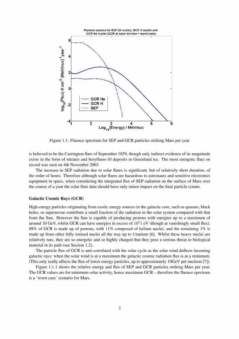
Figure 1.1: Fluence spectrum for SEP and GCR particles striking Mars per year

is believed to be the Carrington flare of September 1859, though only indirect evidence of its magnitudeexists in the form of nitrates and beryllium-10 deposits in Greenland ice. The most energetic flare onrecord was seen on 4th November 2003.

The increase in SEP radiation due to solar flares is significant, but of relatively short duration, ofthe order of hours. Therefore although solar flares are hazardous to astronauts and sensitive electronicsequipment in space, when considering the integrated flux of SEP radiation on the surface of Mars overthe course of a year the solar flare data should have only minor impact on the final particle counts.

Galactic Cosmic Rays (GCR)

High energy particles originating from exotic energy sources in the galactic core, such as quasars, blackholes, or supernovae contribute a small fraction of the radiation in the solar system compared with thatfrom the Sun. However the Sun is capable of producing protons with energies up to a maximum ofaround 10 GeV, whilst GCR can have energies in excess of 1021 eV (though at vanishingly small flux).88% of GCR is made up of protons, with 11% composed of helium nuclei, and the remaining 1% ismade up from other fully ionised nuclei all the way up to Uranium [6]. Whilst these heavy nuclei arerelatively rare, they are so energetic and so highly charged that they pose a serious threat to biologicalmaterial in its path (see Section 1.2).

The particle flux of GCR is anti-correlated with the solar cycle as the solar wind deflects incominggalactic rays: when the solar wind is at a maximum the galactic cosmic radiation flux is at a minimum.(This only really affects the flux of lower energy particles, up to approximately 10GeV per nucleon [7]).

Figure 1.1.1 shows the relative energy and flux of SEP and GCR particles striking Mars per year.The GCR values are for minimum solar activity, hence maximum GCR – therefore the fluence spectrumis a ’worst case’ scenario for Mars.

3

Hadroniccore

Electromagneticcascade

Primary Primary CGR particleCGR particle

π0

γ

e+e-

π−

π+

e+

µ+e-

µ−

γ

n

n

p

p

p

p

n

FluxFlux

Figure 1.2: Diagram illustrating the cascade of secondary particles in the Earth’s atmosphere resultingfrom a single energetic primary particle (e.g. cosmic ray). The graph on the right indicates particle fluxas the particle shower goes deeper into the atmosphere; the peak in the flux is the Pfotzer Maximum(image courtesy of Dartnell)

1.1.2 The Pftozer Maximum

The Earth is largely protected from SEP and GCR thanks to its magnetic field, which deflects incomingcharged particles below an energy of hundreds of MeV, and it’s atmosphere which soaks up most of theenergy from any other incoming particles by a cascade of nuclear interactions.

These interactions, from fragmentation and scattering to direct ionization, produce a large numberof secondary particles which also have relatively high energy, and go on to cause further cascades ofsecondary reactions of their own until the excess kinetic energy is dissipated. The energy of the primaryparticle is therefore bled away at the cost of the generation of a large number of extra secondary particles,giving a high cumulative particle flux which increases with depth through the atmosphere to a maximumknown as the Pfotzer Maximum. After the Pfotzer Maximum particles have insufficient energy left togenerate new secondary particles, and the flux tails off.

On the Earth this Pfotzer Maximum occurs high in the atmosphere, at an altitude of approximately15km. However on Mars the atmosphere is so thin (10-50 mbar atmospheric pressure at the surface,depending on the season) that incoming primary particles are not dissipated very much by the atmo-sphere, and the Pfotzer maximum in fact occurs just below the surface of the planet. In practical termsthis means that in fact the first few centimetres under the surface of Mars are even more inhospitablethan the surface: although UV rays are blocked out, the dense rock gives the first major obstacle tohighly energetic SEP or GCR particles and large numbers of secondary particles saturate that region ofthe surface.

The obvious question is just how far under the surface must one travel before conditions becomesuitable for life? The answer to this depends on what one is looking for. Bacteria may be frozen inthe regolith in a dormant state, accumulating damage over time from the radiation being deposited fromspace. Occasionally a localised thawing of the regolith may occur, which would allow the bacteria toreawaken and allow biological repair mechanisms to reverse some of the accumulated damage from theprevious millennia. Therefore the question of how deep one has to dig to find life depends on how often

4

it is expected that thawing events allow the chance for repair of accumulated damage, as well as thetype of radiation encountered at each depth and the effect of the different types of radiation on differentbiological materials.

1.2 The Biological Effect of Radiation

Radiation can broadly be classified as either ionizing and non-ionizing, and the damage caused to bio-logical material by each group is different. Of the non-ionizing types of radiation, EM radiation at theenergetic end of the spectrum are of prime importance to radiobiology: UV radiation is non-ionizing, butcan cause considerable damage to biological material through promoting usually unfavourable chemicalreactions. X-rays and γ-rays are not ionizing in the sense of strongly ionizing radiation particles such asα particles, but are capable of ionizing biological molecules through photo-excitation, and so are weaklyionizing.

Electromagnetic radiation causes biological damage through photons exciting biological moleculesinto higher energy states than usual, allowing them to undergo chemical reactions which alter theirfunction, generally for the worse. Ultraviolet radiation at wavelengths between about 200nm to 280nm(termed UVC radiation, as distinct from the longer wavelength UVA and UVB) is most damaging to bi-ological material due to the sensitivity of DNA to photons at this wavelength, which cause single-strandbreaks of the DNA double helix or cause single base changes through photochemical reactions with theindividual base molecules. The most significant damage caused by UV is the formation of pyrimidinedimers along the DNA molecule, where the double bond in a pyrimidine base (thymine of cytosine)absorbs a photon, exciting the bond and allowing it to react with a neighbouring pyrimidine base. Theresult is a kink in the DNA helix and reduced interaction with the paired bases of the nucleotides. If leftunrepaired it is likely that transcription proteins will produce errors at this point (transcribing CC to TTis the ’signature’ of UV mutation), leading to incorrectly assembled proteins with loss of function.

X-ray and γ-ray photons can carry enough energy to directly ionize a molecule – that is, an electronis excited not just into an energetic state, but is stripped from the molecule entirely. The molecule is thensignificantly reactive and likely to undergo some chemical reaction which will alter it’s structure. Formost biological molecules such as proteins, structure and function are inter-related, and so even a smallchange in structure can render the molecule useless, or worse still make it directly harmful. In additionX-rays and γ-rays can induce the formation of free-radicals.

Ionizing radiation includes high energy electrons in the form of β- or δ-rays (the difference beingβ-ray electrons are ’primary’ particles whereas delta rays are induced by other types of primary parti-cle); positron radiation produced through nuclear reactions from hadronic primary particles; α particles(ionised Helium nuclei) and all heavier atomic nuclei which can be produced as heavy ions by nuclearfragmentation.

Although ionizing radiation can cause damage through direct impact with biological molecules, bypromoting unfavourable reactions or breaking existing bonds (e.g. single strand breaks in DNA), mostof the damage caused by ionizing radiation is through free-radical production. Since biological tissue islargely composed of water, the passage of an ionizing particle is likely to cause a track of free radicalproduction as water molecules are split by the passing ion. Hydroxyl radicals are extremely reactiveentities and will cause massive damage to any biological molecule it encounters through promotinghighly energetic chemical reactions, such as complete fracture of the DNA double helix, resulting inpotentially massive loss of genetic data. Such damage caused by free radicals is very difficult for acell to reverse, particularly in the case of bacteria where the genetic material freely floats through thecytoplasm, making it especially vulnerable to free radical damage.

In the event that free radicals avoid breaking DNA, they can also cause other types of damage toa cell, causing leakage of enzymes from intracellular compartments; reaction with membrane lipidsleading to change of membrane diffusion dynamics; proteins altered by free radical reactions can im-

5

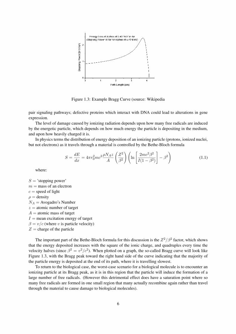
Figure 1.3: Example Bragg Curve (source: Wikipedia

pair signaling pathways; defective proteins which interact with DNA could lead to alterations in geneexpression.

The level of damage caused by ionizing radiation depends upon how many free radicals are inducedby the energetic particle, which depends on how much energy the particle is depositing in the medium,and upon how heavily charged it is.

In physics terms the distribution of energy deposition of an ionizing particle (protons, ionized nuclei,but not electrons) as it travels through a material is controlled by the Bethe-Bloch formula

S =dE

dx= 4πr2

0mc2 ρNAz

A

(Z2

β2

)(ln

[2mc2β2

I(1− β2)

]− β2

)(1.1)

where:

S = ’stopping power’m = mass of an electronc = speed of lightρ = densityNA = Avogadro’s Numberz = atomic number of targetA = atomic mass of targetI = mean excitation energy of targetβ = v/c (where v is particle velocity)Z = charge of the particle

The important part of the Bethe-Bloch formula for this discussion is the Z2/β2 factor, which showsthat the energy deposited increases with the square of the ionic charge, and quadruples every time thevelocity halves (since β2 = v2/c2). When plotted on a graph, the so-called Bragg curve will look likeFigure 1.3, with the Bragg peak toward the right hand side of the curve indicating that the majority ofthe particle energy is deposited at the end of its path, where it is travelling slowest.

To return to the biological case, the worst-case scenario for a biological molecule is to encounter anionizing particle at its Bragg peak, as it is in this region that the particle will induce the formation of alarge number of free radicals. (However this detrimental effect does have a saturation point where somany free radicals are formed in one small region that many actually recombine again rather than travelthrough the material to cause damage to biological molecules).

6

In medical physics this effect can be exploited to beneficial effect through tuning a radiation sourcesuch that the Bragg peak falls on a target region of infected cells, such as a cancerous tumour, to max-imise the dose-on-target while minimising the damage to the healthy outer layers of tissue through whichthe radiation has travelled to reach the tumour.

The exception to the above categorisation of ionizing/non-ionizing radiation is neutron radiationwhich causes damage similar to that caused by energetic protons. This is because neutrons can easilydisplace protons from virtually any atom, as well as cause nuclear fragmentation, so that although theprimary particle itself is not ionizing, the secondary particles it produces are highly ionizing in nature.

1.3 Biological Mechanisms for Repair of Radiation Damage

Clearly the best approach for repair of radiation damage to a cell is to avoid that damage in the first place– hence the evolution of UV-absorbing pigment in human skin which acts as a first line of defence againstUV damage. In the case of ionizing radiation, where free radical production is the prime hazard, a cellcan mitigate the problem to a certain extent by having anti-oxidant molecules available within the cellto ’mop up’ excess free radicals before they have the chance to cause damage. Multi-cellular organismsalso have the advantage that individual damaged cells can be killed without killing the organism as awhole.

However for a simple bacteria these methods are not available, and the cell must cope as best it canwith any damage which occurs.

1.3.1 Reversing UV damage

The pyrimidine dimer (aka. thymine dimer) damage caused by UV interactions can be reversed by aprocess called “nucleotide excision repair” (NER) where a large number of different proteins collaborateto detect damage and clip out around 30 bases around the damaged region. DNA replication enzymesthen re-fill the bases to restore the correct genetic sequence. In humans this is the only method of UVrepair available.

Other non-mammalian organisms have additional methods of repair for UV damage, such as en-donuclease enzymes which are capable of directly removing thymine dimers from the DNA doublehelix, through detecting the weakening in the DNA backbone caused by a pyrimidine dimer.

Photolyase is an enzyme found in prokaryotes and in yeast. It is a light-activated enzyme to repairthymine dimers in a process known as photoreactivation. The photolyase enzyme uses energy absorbedfrom visible light to catalyse the removal of thymine dimer lesions from DNA.

The RecA protein in e. coli is one of the many DNA repair enzymes which contribute to reversingdamage to the DNA molecule; the protein has a homologue in virtually all organisms, making it a highlyubiquitous protein structure. In RecA deficient strains of the bacteria the protein is non-functional,leading to loss of repair ability for UV damage.

1.3.2 Repairing Double-Strand Breaks

Double-strand breaks in DNA, such as those caused by ionizing radiation, can be repaired either byHomologous Recombination (HR) or Non-homologous End Joining (NHEJ). HR uses the homologouspair chromosome to reconstruct the sequence of the broken DNA molecule. NHEJ is less complicatedand less reliable – the ends of the broken molecule are simply stitched back together, with possibleinversion or loss of significant chunks of genetic material.

Deinococcus radiodurans (Figure 1.4) is an interesting bacteria in that it is able to withstand amassive fragmentation of its genetic material through double-strand breaks, and yet still faithfully re-construct the genetic material without loss of function. It is believed that this is due to each cell having

7

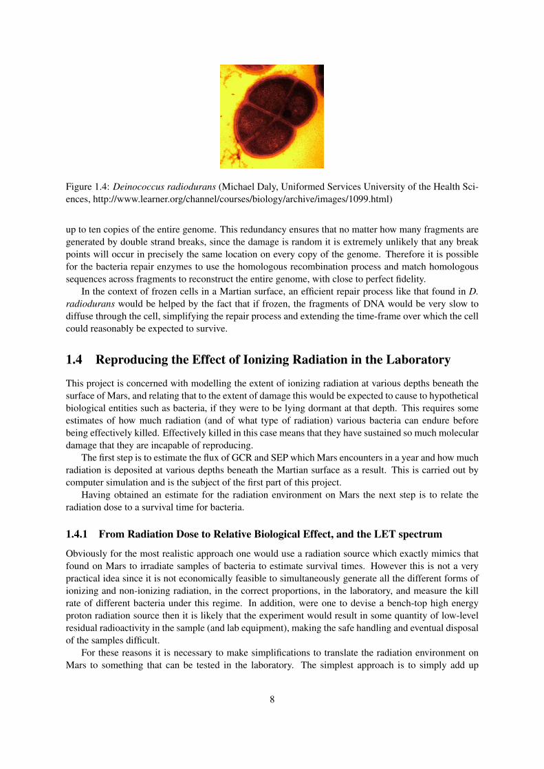
Figure 1.4: Deinococcus radiodurans (Michael Daly, Uniformed Services University of the Health Sci-ences, http://www.learner.org/channel/courses/biology/archive/images/1099.html)

up to ten copies of the entire genome. This redundancy ensures that no matter how many fragments aregenerated by double strand breaks, since the damage is random it is extremely unlikely that any breakpoints will occur in precisely the same location on every copy of the genome. Therefore it is possiblefor the bacteria repair enzymes to use the homologous recombination process and match homologoussequences across fragments to reconstruct the entire genome, with close to perfect fidelity.

In the context of frozen cells in a Martian surface, an efficient repair process like that found in D.radiodurans would be helped by the fact that if frozen, the fragments of DNA would be very slow todiffuse through the cell, simplifying the repair process and extending the time-frame over which the cellcould reasonably be expected to survive.

1.4 Reproducing the Effect of Ionizing Radiation in the Laboratory

This project is concerned with modelling the extent of ionizing radiation at various depths beneath thesurface of Mars, and relating that to the extent of damage this would be expected to cause to hypotheticalbiological entities such as bacteria, if they were to be lying dormant at that depth. This requires someestimates of how much radiation (and of what type of radiation) various bacteria can endure beforebeing effectively killed. Effectively killed in this case means that they have sustained so much moleculardamage that they are incapable of reproducing.

The first step is to estimate the flux of GCR and SEP which Mars encounters in a year and how muchradiation is deposited at various depths beneath the Martian surface as a result. This is carried out bycomputer simulation and is the subject of the first part of this project.

Having obtained an estimate for the radiation environment on Mars the next step is to relate theradiation dose to a survival time for bacteria.

1.4.1 From Radiation Dose to Relative Biological Effect, and the LET spectrum

Obviously for the most realistic approach one would use a radiation source which exactly mimics thatfound on Mars to irradiate samples of bacteria to estimate survival times. However this is not a verypractical idea since it is not economically feasible to simultaneously generate all the different forms ofionizing and non-ionizing radiation, in the correct proportions, in the laboratory, and measure the killrate of different bacteria under this regime. In addition, were one to devise a bench-top high energyproton radiation source then it is likely that the experiment would result in some quantity of low-levelresidual radioactivity in the sample (and lab equipment), making the safe handling and eventual disposalof the samples difficult.

For these reasons it is necessary to make simplifications to translate the radiation environment onMars to something that can be tested in the laboratory. The simplest approach is to simply add up

8

the energy dose from each type of radiation at a given depth on the surface of Mars, as calculated bycomputer simulation. This gives a total radiation dose (expressed in Grays per cm2, per year). This dosecan then be administered in the form of any other radiation in the lab, typically γ-radiation. This is thecrudest level of simplification since it neglects the differing biological implications of exposure to eachvariety of radiation.

A slightly improved method is to derive the Relative Biological Effect (RBE) of the radiation envi-ronment which is defined as the dose of γ-radiation which would produce equivalent biological effect.This is worked out by arbitrary scaling of each type of radiation source - for example an alpha particle isdeemed to be equivalent to twenty times its dose in γ-rays, so all radiation doses originating from alphaparticles are multiplied by twenty.

γ-rays are chosen as the benchmark radiation type since they are relatively easy to produce in smallquantities in the lab from readily available radionuclides. γ-rays are sufficiently penetrating that theycan interact with biological samples within glass containers, unlike laboratory produced alpha radiationwhich is unable to penetrate so much as a single sheet of paper. In addition γ-sources do not induceradioactivity in the sample, so they are one of the safer forms of radioactivity with which to work,assuming simple common-sense safety precautions are followed.

The disadvantage of the RBE is that the scale factors are empirically derived from radiation experi-ments on eukaryotic cells, for example experiments carried out by the medical physics community whoare primarily interested on the effect of radiation on human patients. Therefore these scale factors arenot necessarily relevant when it comes to considering prokaryotes such as bacteria, where the geneticmaterial is not confined within a nuclear envelope, and where different methods of repair mechanismsexist depending on the type of damage sustained. The RBE makes no allowance for the effect of rate ofenergy deposition on biological effect – for example the exchange rate of alpha particles to γ-rays willincrease as the particle reaches the Bragg peak.

A more realistic approach to marrying radiation doses (in energy units per year) to a dosage of γ-radiation (in time units of exposure) is to make use of the Linear Energy Transfer (LET) spectrum of theradiation environment. The LET spectrum expresses the dose delivered in terms of the energy depositedper unit length, normalised to the total dosage, rather than the net dose itself. This is a better quantityto consider since it effectively takes into account the rate of energy deposition of the radiation particle,which for ionizing radiation will be equivalent to the rate of production of damaging free radicals.

Thus a slow moving, highly charged Fe56 ion (depositing energy as its Bragg peak) will have ex-tremely high LET since it is depositing energy at a massive rate over a short distance, causing enormousbiological damage. The same Fe56 ion earlier in its path with higher kinetic energy may in fact registera lower LET if it has not yet reached the Bragg peak, since although it is more energetic, it is not givingup so much energy to the surrounding tissue. In contrast a relatively high-energy γ-ray may have a lowLET since it continuously deposits its energy as it travels long distances through the material, and willnot cause nearly so much biological damage.

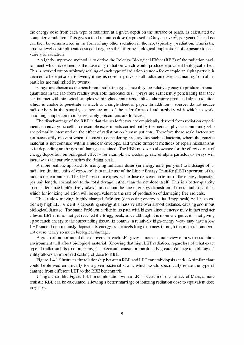
A graph of proportion of dose delivered at each LET gives a more accurate view of how the radiationenvironment will affect biological material. Knowing that high LET radiation, regardless of what exacttype of radiation it is (proton, γ-ray, fast electron), causes proportionally greater damage to a biologicalentity allows an improved scaling of dose to RBE.

Figure 1.4.1 illustrates the relationship between RBE and LET for arabidopsis seeds. A similar chartcould be derived empirically for a given bacterial strain, which would specifically relate the type ofdamage from different LET to the RBE benchmark.

Using a chart like Figure 1.4.1 in combination with a LET spectrum of the surface of Mars, a morerealistic RBE can be calculated, allowing a better marriage of ionizing radiation dose to equivalent dosein γ-rays.

9

Figure 1.5: RBE vs. LET for Arabidopsis seeds

1.4.2 From γ-Radiation to Survival Curves

The previous section explains how it is possible to convert a given radiation spectrum (measured in termsof LET rather than raw energy deposition) into an equivalent dose of γ-radiation. The final step is toestimate how rapidly bacteria will become effectively killed (i.e. incapable of producing viable daughtercells) given the yearly dose of radiation.

The technique is to simply irradiate a frozen sample of a given bacteria with γ-radiation equivalent toa number of years exposure to radiation, and to then thaw the bacteria, spread them on agar impregnatedwith nutrient broth, and to estimate the fraction of bacteria which survived the whole process.

10

Chapter 2

Modelling Extraterrestrial RadiationEnvironments

This chapter discusses the Geant4 framework used to model the radiation environment on the surface ofMars, its limitations, and the model parameters used for this project.

2.1 Geant4

Geant4 is a modelling framework [8] developed by a large community of scientists to simulate thepassage of particles through matter. The toolkit has a wide range of possible applications, includingspace science.

The ATMOCOSMICS program is an application based upon the Geant4 toolkit developed by Lau-rent Desorgher et al. [9] to simulate the interaction of cosmic rays with the Earth’s atmosphere. Dartnellextended the code to simulate the effect of solar and galactic radiation on the atmosphere and surface ofMars, and used it to calculate energy deposition profiles for a Martian year at various levels beneath theMartian surface [10] [7].

This project takes code supplied by Dartnell and extends it to calculate not only the energy depositionprofile, but the LET spectrum on and beneath the Martian surface.

Geant4 is a Monte Carlo type modelling tool: successive simulated particles are independent ofone another, and the interactions experienced by each particle (and hence energy deposition profile ofeach particle) is random within the bounds set by hard-coded probabilities defined in Geant4 (nuclearinteraction cross-sections). The output of the simulation of a single particle is the energy depositionprofile of that particle (and any secondary particles it produces) as it travels through the Geant4 world.A second particle of similar energy will produce a similar but probably not identical deposition profile(due to the stochastic nature of the modelling). As further particles are simulated the statistics of thedeposition profile should gradually converge to a reasonable approximation of reality.

Since each primary particle within Geant4 can be treated independently, and results from many par-ticles are amalgamated to produce the final deposition profile, the process lends itself well to paralleli-sation across multiple computers. The code supplied by Dartnell was modified to run on the CoMPLEXXGrid (a network of Apple Mac computers which donate idle CPU time to running parallel processes).A centralised MySQL database was used to collate the results to allow maximum flexibility in post-processing of the results.

2.1.1 Limitations of Geant4

The statistical parameters within Geant4 which control the likelihood of each type of particle interactionobviously have an enormous effect on the accuracy and validity of the results produced by Geant4. The

11

scientists who regularly update Geant4 continually improve the correspondence between Geant4 andreality by updating the models and parameters within Geant4.

Unfortunately from a programming point of view the authors of Geant4 do not seem to prioritizebackwards compatibility of their code: the program supplied by Dartnell and Desorgher was originallywritten for Geant4 version 4.7.0 (released February 2005), and does not work with any later versionsof the Geant4 framework. Using the latest version of Geant4 (4.8.3) the code does not at first compilewithout some minor modifications. Once compiled the code produces runtime errors; modificationsto resolve these errors resulted in a program which entered a seemingly infinite loop in the steppingroutines within Geant4.

Without more in-depth knowledge of the workings of the Geant4 and ATMOCOS sections of theprogram, it is necessary to continue using an out-dated version of the framework.

In addition to the version limitation discussed above, Geant4 also has an energy limitation of 10GeV per nucleon for ionic primary particles, and ionic primaries beyond Carbon-12 are not supported.Exceeding these limits is possible, but the authors of Geant4 make no guarantees as to the validity of theresulting simulation. This latter limitation is particularly irritating for assessing the impact of GCR onbiological matter since it disallows the simulation of Iron nuclei (Fe56 ions). As mentioned previouslythe GCR spectrum is composed mainly of hydrogen and helium nuclei, with only relatively low fluxof heavier ions. However there is a significant peak of flux around carbon and iron, which should notbe neglected due to the relatively high ionic charges they carry (which appears as a squared term in theBethe-Bloch formula). Therefore although the particle flux of Fe56 is orders of magnitude lower thanthat of GCR protons, they cannot be neglected.

With a limit of 10 GeV per nucleon, the most energetic GCR He nuclei which can be directlysimulated have a total energy of 40 GeV, which is below the energy at which the GCR particle fluxbecomes negligible. It is possible to ’fake’ the higher energy He nuclei by simulating four energeticprotons in their place and multiplying the resultant energy depositions by a weighting factor. For thisproject, due to time constraints, simulations were carried out for H nuclei (protons) only up to 500 GeV,and He nuclei up to the Geant4 limit of 40GeV (total energy), and no proton “fill-in” was attempted.(It would be interesting to extend the simulations beyond the Geant4 limit and compare the results withresults where protons are used in place of He nuclei, to see the extent to which they agree or disagree,however this is beyond the scope of this project.)

2.1.2 Model Parameters

The model was initialized with a column of Martian atmosphere and dry topsoil. 1

The regolith was set to record depositions in ten centimeter layers – that is, deposition events wereassigned to a depth beneath the surface discretized into 10 cm lengths.

The range of primary particle energies (10 MeV to 1 TeV – 5 orders of magnitude) was divided into500 logarithmically equal sized bins (a constant ratio between upper bound and lower bound of each bin,such that the base-10 logartihm of this ratio = 0.01 (5 orders of magnitude divided by 500 bins)). Foreach energy bin a number of primary particles were simulated such that the energy and LET depositionprofile obtained by the aggregate set of results was thought to representative.

It should be noted that the quantity of prime interest is the energy and LET deposition profile ofall resultant particles from a primary particle of given energy, not just the deposition of the primaryitself (though this will obviously contribute to the overall profile). Therefore the number of primaryparticles which must be simulated for a statistically accurate representation of the deposition profiledepends on the number of secondary particles which the primary can be expected to generate – high

1atmosphere composition by mass: CO2: 95.47%, N2: 2.7%, Ar: 1.6%, O2: 0.13%, CO: 0.07%, H2O: 0.03%. Regolithcomposition by mass: SiO2: 42,65%, Fe2O3: 22.3 %, MgO: 8.69%, Al2O3: 7.98%, SO3: 6.79%, CaO: 6.53%, TiO2: 1.01%,P2O5: 0.98%, K2O: 0.61%, Cl: 0.55%, MnO: 0.52%, Cr2O3: 0.30%

12

energy primaries produce vastly more secondary particles than low energy primaries, therefore fewerhigh energy primaries need be simulated for an accurate deposition profile.

The best method to ensure high quality statistically plausible results would be to continuously buildthe deposition histogram every time a primary is simulated, and to keep simulating primaries until thefurther simulation of a primary particle of any energy does not significantly alter the shape of the his-togram. At this point one could be confident that the deposition data is a good representation of theactual distribution.

For this project a simpler approach was taken where as many primary particles were simulated aswas feasible in the time available, with fewer high energy primaries than low energy primaries beingsimulated. The final spectrum obtained is believed to be statistically valid – adding the results from asmall number of extra primaries to the histogram made no noticeable difference. However this methodwas probably a little wasteful of computing resources; a more statistically rigorous approach would beappropriate for future simulations.

2.1.3 Data Collection

The results were collected into a MySQL database which aggregated deposition data according to:

• layer at which deposition occurred

• energy of the primary particle (in MeV)

• LET of the depositing particle (binned between 10−6 and 104 keV/µm in 1000 evenly logarithmi-cally spaced bins)

• type of depositing particle (electron, proton, gamma, heavy ion, etc.)

(The cumulative energy deposited in that LET bin was also recorded, in order to allow dose-normalisedLET spectra to be calculated later, should that be required.)

The spectrum of primaries simulated was recorded separately. Once a large number of primaryparticles had been simulated across all energy bins (corresponding to no specific solar or cosmic ra-diation spectra), the histogram counts for each energy level were normalised, to give a “histogram ofhistograms” which contained the entire LET spectrum for every combination of layer and secondaryparticle type, for a single primary particle of each energy bin.

From the normalised data, a LET spectrum at any layer for any secondary particle type, due to anycombination of primaries could be calculated by summing the individual LET spectra correspondingto the input primary energy histogram (e.g. that for a year of SEP radiation, or for the helium nucleuscomponent of GCR).

The advantage of this approach is that the maximum amount of data is extracted from the simulationsuch that any input spectra can be ’simulated’ just be re-scaling the collected data, rather than re-runningthe simulations again which would consume further computing power.

The distinct disadvantage is a somewhat complicated database structure to handle the results, witha single table holding most of the data which grows to quite enormous size. The enormous size is notin itself a major problem (hard disk space is very cheap per GB), however since the database table isindexed for each of the variables listed above, the computational cost of actually extracting the results byrunning queries on the database becomes increasingly large. This problem can be mitigated by loweringthe resolution of the energy bins for primary particles, or lowering the resolution of the LET bins fordeposition events, or by collecting LET data summed for certain collections of secondary particle, ratherthan collecting them individually.

13

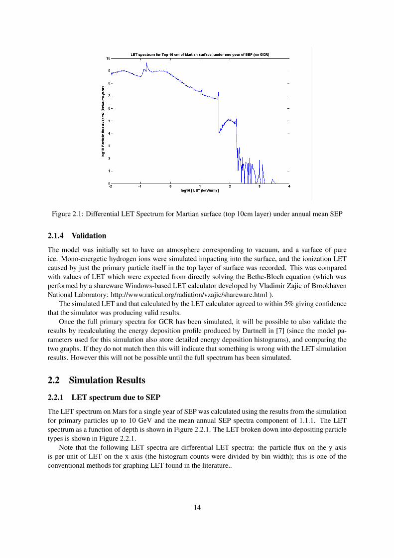
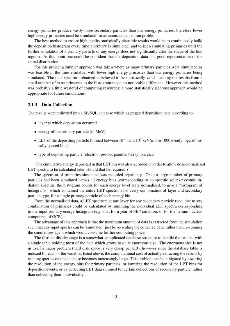
Figure 2.1: Differential LET Spectrum for Martian surface (top 10cm layer) under annual mean SEP

2.1.4 Validation

The model was initially set to have an atmosphere corresponding to vacuum, and a surface of pureice. Mono-energetic hydrogen ions were simulated impacting into the surface, and the ionization LETcaused by just the primary particle itself in the top layer of surface was recorded. This was comparedwith values of LET which were expected from directly solving the Bethe-Bloch equation (which wasperformed by a shareware Windows-based LET calculator developed by Vladimir Zajic of BrookhavenNational Laboratory: http://www.ratical.org/radiation/vzajic/shareware.html ).

The simulated LET and that calculated by the LET calculator agreed to within 5% giving confidencethat the simulator was producing valid results.

Once the full primary spectra for GCR has been simulated, it will be possible to also validate theresults by recalculating the energy deposition profile produced by Dartnell in [7] (since the model pa-rameters used for this simulation also store detailed energy deposition histograms), and comparing thetwo graphs. If they do not match then this will indicate that something is wrong with the LET simulationresults. However this will not be possible until the full spectrum has been simulated.

2.2 Simulation Results

2.2.1 LET spectrum due to SEP

The LET spectrum on Mars for a single year of SEP was calculated using the results from the simulationfor primary particles up to 10 GeV and the mean annual SEP spectra component of 1.1.1. The LETspectrum as a function of depth is shown in Figure 2.2.1. The LET broken down into depositing particletypes is shown in Figure 2.2.1.

Note that the following LET spectra are differential LET spectra: the particle flux on the y axisis per unit of LET on the x-axis (the histogram counts were divided by bin width); this is one of theconventional methods for graphing LET found in the literature..

14

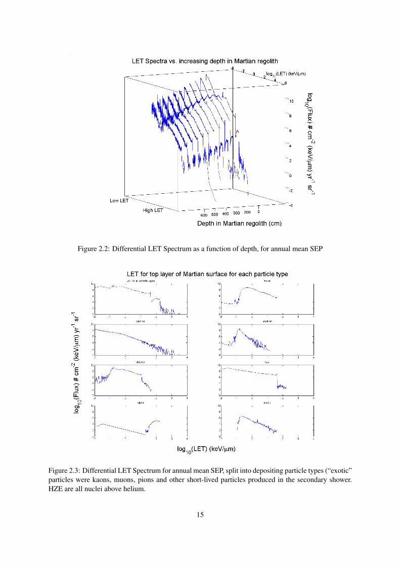
Figure 2.2: Differential LET Spectrum as a function of depth, for annual mean SEP

Figure 2.3: Differential LET Spectrum for annual mean SEP, split into depositing particle types (“exotic”particles were kaons, muons, pions and other short-lived particles produced in the secondary shower.HZE are all nuclei above helium.

15

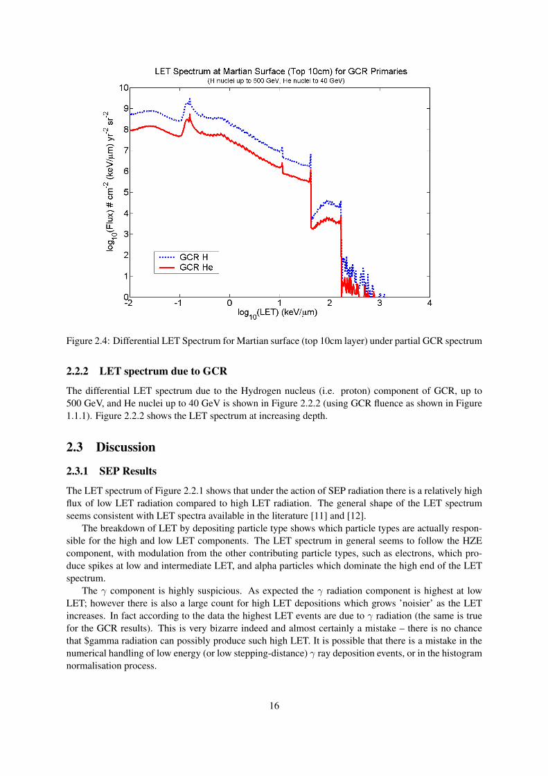
Figure 2.4: Differential LET Spectrum for Martian surface (top 10cm layer) under partial GCR spectrum

2.2.2 LET spectrum due to GCR

The differential LET spectrum due to the Hydrogen nucleus (i.e. proton) component of GCR, up to500 GeV, and He nuclei up to 40 GeV is shown in Figure 2.2.2 (using GCR fluence as shown in Figure1.1.1). Figure 2.2.2 shows the LET spectrum at increasing depth.

2.3 Discussion

2.3.1 SEP Results

The LET spectrum of Figure 2.2.1 shows that under the action of SEP radiation there is a relatively highflux of low LET radiation compared to high LET radiation. The general shape of the LET spectrumseems consistent with LET spectra available in the literature [11] and [12].

The breakdown of LET by depositing particle type shows which particle types are actually respon-sible for the high and low LET components. The LET spectrum in general seems to follow the HZEcomponent, with modulation from the other contributing particle types, such as electrons, which pro-duce spikes at low and intermediate LET, and alpha particles which dominate the high end of the LETspectrum.

The γ component is highly suspicious. As expected the γ radiation component is highest at lowLET; however there is also a large count for high LET depositions which grows ’noisier’ as the LETincreases. In fact according to the data the highest LET events are due to γ radiation (the same is truefor the GCR results). This is very bizarre indeed and almost certainly a mistake – there is no chancethat $gamma radiation can possibly produce such high LET. It is possible that there is a mistake in thenumerical handling of low energy (or low stepping-distance) γ ray deposition events, or in the histogramnormalisation process.

16

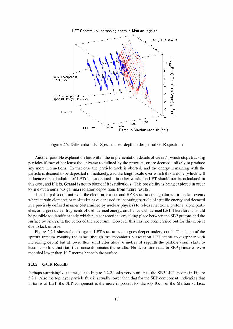
Figure 2.5: Differential LET Spectrum vs. depth under partial GCR spectrum

Another possible explanation lies within the implementation details of Geant4, which stops trackingparticles if they either leave the universe as defined by the program, or are deemed unlikely to produceany more interactions. In that case the particle track is aborted, and the energy remaining with theparticle is deemed to be deposited immediately, and the length scale over which this is done (which willinfluence the calculation of LET) is not defined – in other words the LET should not be calculated inthis case, and if it is, Geant4 is not to blame if it is ridiculous! This possibility is being explored in orderto rule out anomalous gamma radiation depositions from future results.

The sharp discontinuities in the electron, exotic, and HZE spectra are signatures for nuclear eventswhere certain elements or molecules have captured an incoming particle of specific energy and decayedin a precisely defined manner (determined by nuclear physics) to release neutrons, protons, alpha parti-cles, or larger nuclear fragments of well defined energy, and hence well defined LET. Therefore it shouldbe possible to identify exactly which nuclear reactions are taking place between the SEP protons and thesurface by analysing the peaks of the spectrum. However this has not been carried out for this projectdue to lack of time.

Figure 2.2.1 shows the change in LET spectra as one goes deeper underground. The shape of thespectra remains roughly the same (though the anomalous γ radiation LET seems to disappear withincreasing depth) but at lower flux, until after about 6 metres of regolith the particle count starts tobecome so low that statistical noise dominates the results. No depositions due to SEP primaries wererecorded lower than 10.7 metres beneath the surface.

2.3.2 GCR Results

Perhaps surprisingly, at first glance Figure 2.2.2 looks very similar to the SEP LET spectra in Figure2.2.1. Also the top layer particle flux is actually lower than that for the SEP component, indicating thatin terms of LET, the SEP component is the more important for the top 10cm of the Martian surface.

17

However on reflection this is not such a surprising result: the SEP primary particle flux is an order ofmagnitude higher than the GCR flux for low energies. Furthermore, the high energy GCR particlesshould not be expected to produce much effect on LET at the top layer since they should be travellingtoo fast to be depositing much energy by ionization – their Bragg peak will lie a few layers below thesurface, as will the Pfotzer maximum (although one would expect considerable backscatter of radiationparticles).

From Figure 2.2.2 this does indeed seem to be the case. The GCR particles penetrate much deeperinto the ground than the SEP particles and soon dominate the LET spectrum, even though this simulationis only a partial GCR spectrum with limited energy primaries.

It is also clear that low numbers of energetic primary GCR particles are capable of producing a sig-nificant secondary cascade; what the primary particles lack in numbers, they make up for in secondaryparticle generation. It is notable the pattern of signature nuclear interactions (spikes in the LET spec-trum) are the same for both SEP and GCR components – this would seem to indicate that the shapeof the LET spectrum is determined by the chemical makeup of the Martian surface, which producescharacteristic nuclear fragmentation and scattering when bombarded with ionizing particles. The energyof the primary particles does not therefore control the LET spectrum itself, but rather controls the depthinto the regolith to which the LET spectrum extends.

Whilst LET is the biologically relevant parameter of interest, the total energy deposited is obviouslystill important. Therefore a possibly more useful graph may be the LET spectrum normalised by energydeposited at that LET as a fraction of the total energy deposition for all particles. This would give adosage-normalised LET spectrum, which includes both the biologically important factors of LET andenergy.

18

Chapter 3

Experimental Methods

Having calculated a LET spectrum for the surface and subsurface of Mars by simulation with the Geant4framework, the next step is to quantify the effect of that radiation on biological material. From this it ispossible to estimate the survival time of bacteria frozen beneath the Martian surface.

Unfortunately for this project we have access to neither Martian bacteria (since they have never beendiscovered!) nor a source of ionizing radiation, relating the LET spectrum to the kill-rate of life on Marsis a little tricky. The compromise is to use “extremophile” bacteria isolated from soil samples takenfrom the Antarctic as substitutes for the hypothetical Martian bacteria, and to use desiccation and UVCradiation in place of ionizing radiation.

The aim of the project is to find a correlation between the resistance of Antarctic bacteria to UVC,desiccation, and γ radiation. Ideally some combination of UVC and desiccation exposure will provide agood estimator of γ radiation resistance. Having scaled the LET spectrum on Mars to some equivalentdose of γ radiation (via the RBE, or Q-factor), it would then be possible to make a guess about how longthe Antarctic bacteria could survive on Mars, without having to resort to the use of ionizing radiation inthe lab.

The experimental methods used to assess UVC and desiccation resistance are described in the fol-lowing sections, and roughly follow the experimental methods outlined in [13].

3.1 Bacterial Test Strains

Four strains of Antarctic bacteria isolated by Samantha Whiting as part of her PhD thesis [14] werechosen as test bacteria – two of these were found underneath an algal mat (Pseudomonas sp. andPsychrobacter aquatica), and two from an exposed location in the Miers Valley (Bacillus sp. and Strep-tomyces sp.). The samples were chosen to give a range of ’extremity’ in the environment in which thebacteria were found – the two from under the algal mat were subject to less harsh conditions than thosefound in the exposed environment. At the same time these bacteria also all grow on the same media atapproximately the same rate, simplifying things from an experimental point of view.

A further three strains of Antarctic bacteria (labelled LD7, LD10 and LD27) along with a sample ofD. radiodurans, were provided by Lewis Dartnell along with recently measured γ-radiation resistancedata [unpublished, Dartnell]. In addition to this a sample of ’Top10’ strain e. coli was supplied by SteveBranston. All of these strains except the LD27 strain grow at a reasonable rate using the same media asthe Miers Valley bacteria, again simplifying the experimental process. The LD7, LD10, LD27 bacteriawere recently identified by Dartnell using 16S phylogeny as being Brevundimonas sp., Rhodococcussp./Nocardiaceae sp., and Pseudomonas sp. respectively.

The sample of D. radiodurans was included as a benchmark bacteria of known high radiation resis-tance. At the opposite end of the resistance spectrum is the “Top10” e. coli which is a strain of which

19

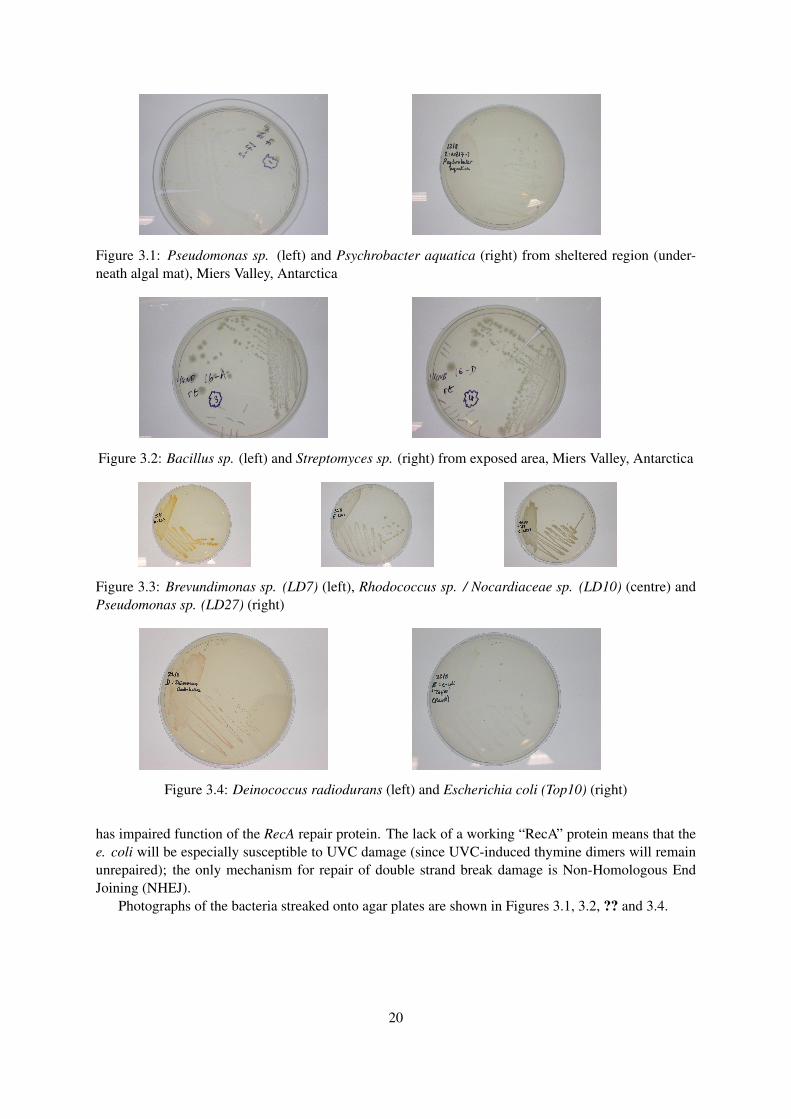
Figure 3.1: Pseudomonas sp. (left) and Psychrobacter aquatica (right) from sheltered region (under-neath algal mat), Miers Valley, Antarctica

Figure 3.2: Bacillus sp. (left) and Streptomyces sp. (right) from exposed area, Miers Valley, Antarctica

Figure 3.3: Brevundimonas sp. (LD7) (left), Rhodococcus sp. / Nocardiaceae sp. (LD10) (centre) andPseudomonas sp. (LD27) (right)

Figure 3.4: Deinococcus radiodurans (left) and Escherichia coli (Top10) (right)

has impaired function of the RecA repair protein. The lack of a working “RecA” protein means that thee. coli will be especially susceptible to UVC damage (since UVC-induced thymine dimers will remainunrepaired); the only mechanism for repair of double strand break damage is Non-Homologous EndJoining (NHEJ).

Photographs of the bacteria streaked onto agar plates are shown in Figures 3.1, 3.2, ?? and 3.4.

20

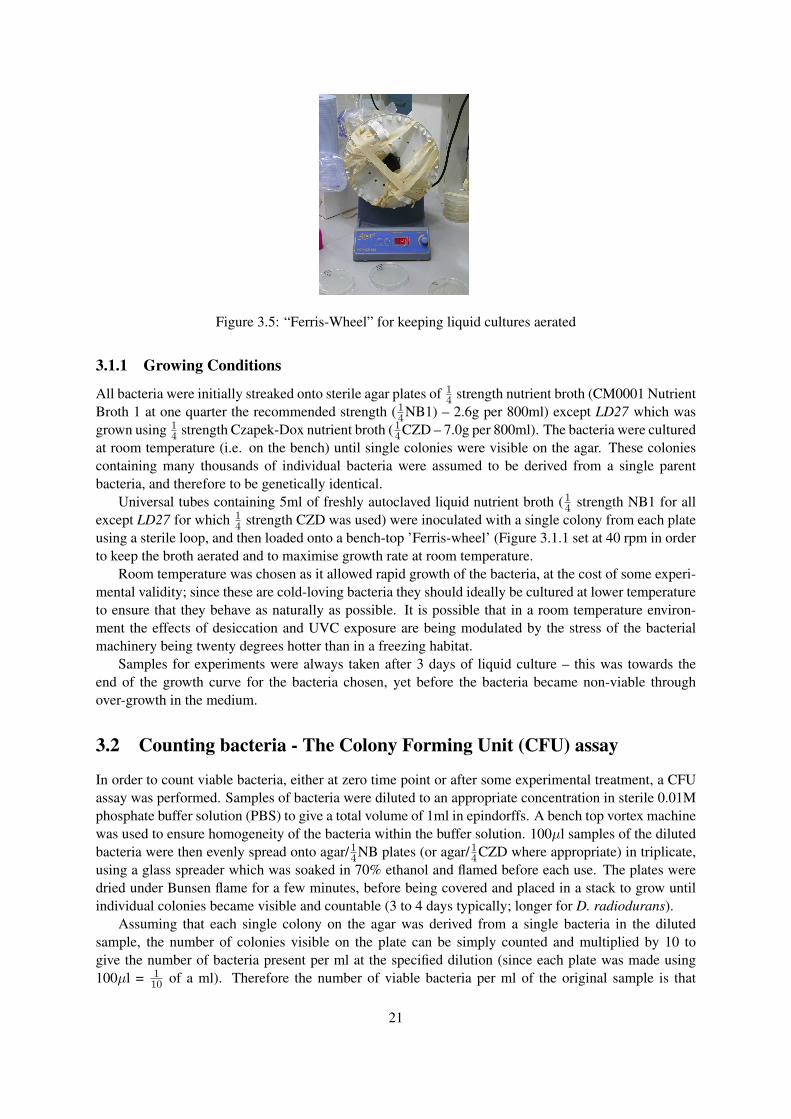
Figure 3.5: “Ferris-Wheel” for keeping liquid cultures aerated

3.1.1 Growing Conditions

All bacteria were initially streaked onto sterile agar plates of 14 strength nutrient broth (CM0001 Nutrient

Broth 1 at one quarter the recommended strength (14NB1) – 2.6g per 800ml) except LD27 which was

grown using 14 strength Czapek-Dox nutrient broth (1

4CZD – 7.0g per 800ml). The bacteria were culturedat room temperature (i.e. on the bench) until single colonies were visible on the agar. These coloniescontaining many thousands of individual bacteria were assumed to be derived from a single parentbacteria, and therefore to be genetically identical.

Universal tubes containing 5ml of freshly autoclaved liquid nutrient broth (14 strength NB1 for all

except LD27 for which 14 strength CZD was used) were inoculated with a single colony from each plate

using a sterile loop, and then loaded onto a bench-top ’Ferris-wheel’ (Figure 3.1.1 set at 40 rpm in orderto keep the broth aerated and to maximise growth rate at room temperature.

Room temperature was chosen as it allowed rapid growth of the bacteria, at the cost of some experi-mental validity; since these are cold-loving bacteria they should ideally be cultured at lower temperatureto ensure that they behave as naturally as possible. It is possible that in a room temperature environ-ment the effects of desiccation and UVC exposure are being modulated by the stress of the bacterialmachinery being twenty degrees hotter than in a freezing habitat.

Samples for experiments were always taken after 3 days of liquid culture – this was towards theend of the growth curve for the bacteria chosen, yet before the bacteria became non-viable throughover-growth in the medium.

3.2 Counting bacteria - The Colony Forming Unit (CFU) assay

In order to count viable bacteria, either at zero time point or after some experimental treatment, a CFUassay was performed. Samples of bacteria were diluted to an appropriate concentration in sterile 0.01Mphosphate buffer solution (PBS) to give a total volume of 1ml in epindorffs. A bench top vortex machinewas used to ensure homogeneity of the bacteria within the buffer solution. 100µl samples of the dilutedbacteria were then evenly spread onto agar/1

4NB plates (or agar/14CZD where appropriate) in triplicate,

using a glass spreader which was soaked in 70% ethanol and flamed before each use. The plates weredried under Bunsen flame for a few minutes, before being covered and placed in a stack to grow untilindividual colonies became visible and countable (3 to 4 days typically; longer for D. radiodurans).

Assuming that each single colony on the agar was derived from a single bacteria in the dilutedsample, the number of colonies visible on the plate can be simply counted and multiplied by 10 togive the number of bacteria present per ml at the specified dilution (since each plate was made using100µl = 1

10 of a ml). Therefore the number of viable bacteria per ml of the original sample is that

21

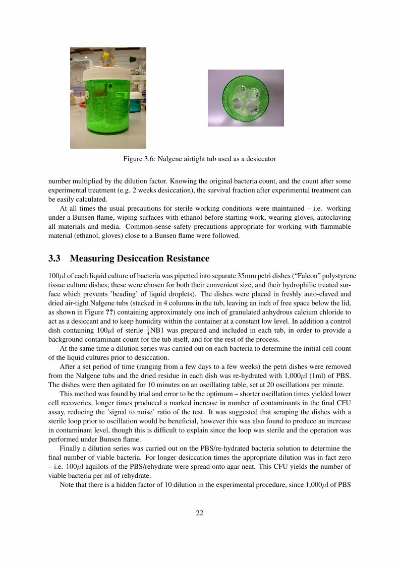
Figure 3.6: Nalgene airtight tub used as a desiccator

number multiplied by the dilution factor. Knowing the original bacteria count, and the count after someexperimental treatment (e.g. 2 weeks desiccation), the survival fraction after experimental treatment canbe easily calculated.

At all times the usual precautions for sterile working conditions were maintained – i.e. workingunder a Bunsen flame, wiping surfaces with ethanol before starting work, wearing gloves, autoclavingall materials and media. Common-sense safety precautions appropriate for working with flammablematerial (ethanol, gloves) close to a Bunsen flame were followed.

3.3 Measuring Desiccation Resistance

100µl of each liquid culture of bacteria was pipetted into separate 35mm petri dishes (“Falcon” polystyrenetissue culture dishes; these were chosen for both their convenient size, and their hydrophilic treated sur-face which prevents ’beading’ of liquid droplets). The dishes were placed in freshly auto-claved anddried air-tight Nalgene tubs (stacked in 4 columns in the tub, leaving an inch of free space below the lid,as shown in Figure ??) containing approximately one inch of granulated anhydrous calcium chloride toact as a desiccant and to keep humidity within the container at a constant low level. In addition a controldish containing 100µl of sterile 1

4NB1 was prepared and included in each tub, in order to provide abackground contaminant count for the tub itself, and for the rest of the process.

At the same time a dilution series was carried out on each bacteria to determine the initial cell countof the liquid cultures prior to desiccation.

After a set period of time (ranging from a few days to a few weeks) the petri dishes were removedfrom the Nalgene tubs and the dried residue in each dish was re-hydrated with 1,000µl (1ml) of PBS.The dishes were then agitated for 10 minutes on an oscillating table, set at 20 oscillations per minute.

This method was found by trial and error to be the optimum – shorter oscillation times yielded lowercell recoveries, longer times produced a marked increase in number of contaminants in the final CFUassay, reducing the ’signal to noise’ ratio of the test. It was suggested that scraping the dishes with asterile loop prior to oscillation would be beneficial, however this was also found to produce an increasein contaminant level, though this is difficult to explain since the loop was sterile and the operation wasperformed under Bunsen flame.

Finally a dilution series was carried out on the PBS/re-hydrated bacteria solution to determine thefinal number of viable bacteria. For longer desiccation times the appropriate dilution was in fact zero– i.e. 100µl aquilots of the PBS/rehydrate were spread onto agar neat. This CFU yields the number ofviable bacteria per ml of rehydrate.

Note that there is a hidden factor of 10 dilution in the experimental procedure, since 1,000µl of PBS

22

Figure 3.7: UV Sterilising Cabinet used to test bacteria UVC resistance

is used to rehydrate a sample originally held in a 100µl volume of liquid. Therefore the calculation oftotal viable cells per ml of rehydrate is divided by the viable cells in 0.1ml of liquid culture.

3.4 Measuring Ultraviolet Radiation (UVC) Resistance

The UVC resistance of bacteria was tested by placing 500µl samples of the liquid cultures of bacteriainto 35mm tissue culture petri dishes (as used for the desiccation experiment). Having taken a dilutionseries to determine initial cell count for each strain 1 the dishes were placed in a UVC sterilising cabinet,Figure 3.4 (previously wiped with Virkon and turned on for several hours to remove contaminants). Thedishes were located directly underneath the UV striplight at the back of the cabinet, and the UV lampswitched on. After set exposure times 10µl aquilots were removed from each petri dish, and a CFUassay performed as described previously.

No special precautions were taken to avoid repair by photoreactivation mechanisms during the ex-periment itself as it was decided that this would overly complicate the procedure. In addition, the aimwas to measure overall resistance to UVC, and the extent to which each bacteria is capable of repairby photoreactivation is ’fair game’ as far as this project is concerned. However, to avoid differing lightconditions while growing on the agar plates following CFU assay, the stack of plates was wrapped infoil for the growth period.

The low surface tension provided by the hydrophilic surface of the petri dish was especially impor-tant for this experiment since it was desirable to have a single thin layer of liquid to expose to UV light.A thin layer is essential to avoid ’self-shielding’ where bacteria suspended in the top layer of the liquidabsorb the full effect of the UVC radiation and shield those bacteria below them in the liquid, leading todistorted results. 500µl was found to be the minimum volume of liquid which would form such a thinsingle layer.

1in practice the same t=0 series was used for UV and desiccation to avoid duplication of work and waste of materials –i.e. after carrying out an initial cell count for a set of bacteria entering the desiccator, a UV test was also carried out to makemaximum use of the initial cell count results

23

Chapter 4

Experimental Results

4.1 Desiccation Resistance

Recovery Efficiency

In order to ensure that the recovery process of rehydrating the bacteria was reasonably efficient, anexperiment was carried out whereby a desiccated sample of Brevundimonas sp. 1 was rehydrated in theusual way above and a CFU assay performed. The remaining liquid in the petri dish (PBS and rehydratedbacteria) was discarded, and another 1000µl of PBS pipetted into the dish, which was oscillated for afurther 10 minutes at 20 osc./min. The CFU assay was repeated (at zero dilution) and compared withthe first CFU results, in order to estimate the proportion of viable cells which remained attached to thepetri dish during the first rehydration process.

The rehydration process was found to be approximately 90% effective: the second rinse produced acell count one tenth that of the initial rehydration. The 90% efficiency was used to correct the results byassuming that the final CFU counts represented only 90% of the bacteria which survived the desiccationprocess.

Controls

The control dishes in the desiccators were hydrated in the same way as the test dishes in order to assessthe level of background contamination. In all cases the control plates contained no more than 8 contam-inant colonies; furthermore often the contaminants had a fungal rather than bacterial appearance, and inany case did not resemble the distinctive appearance of the actual test bacteria, leading to no confusionbetween contamination and actual bacteria. There was no cross-contamination of sample bacteria withinthe desiccator.

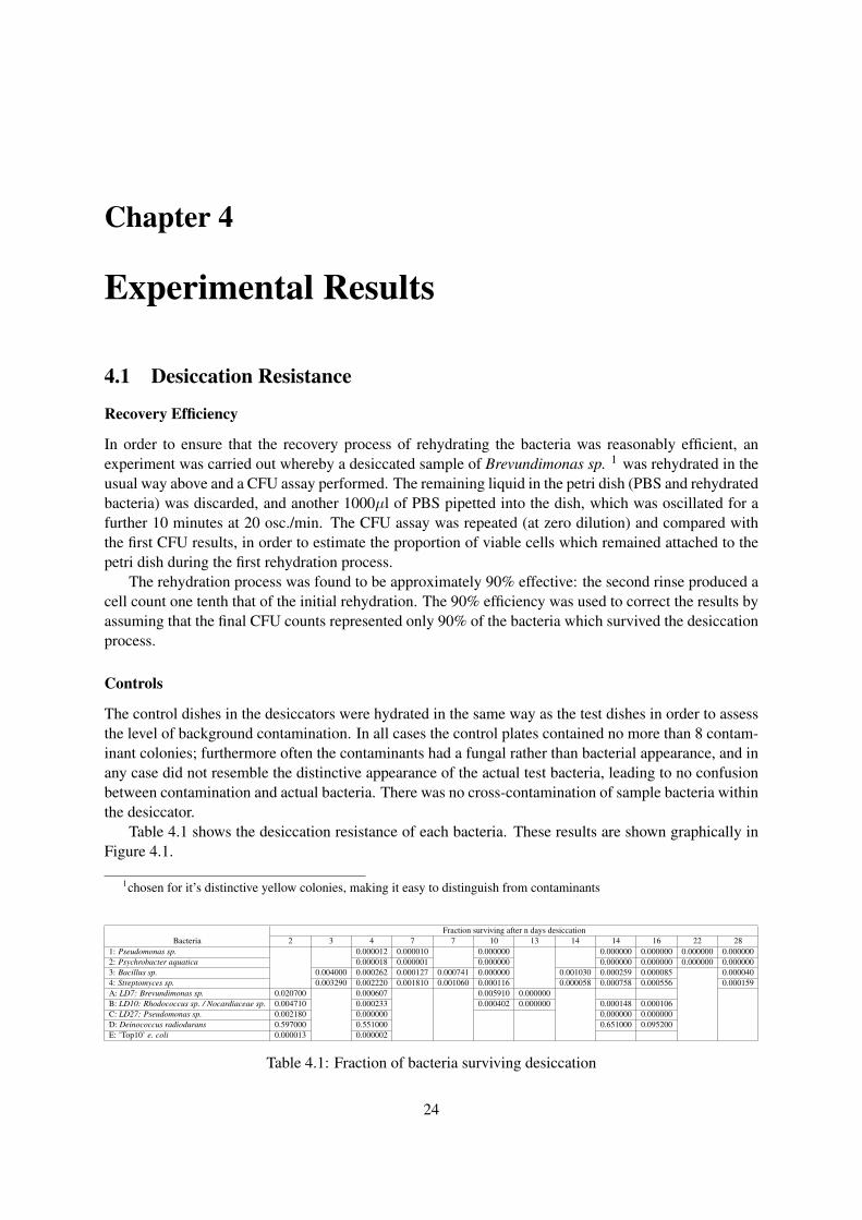
Table 4.1 shows the desiccation resistance of each bacteria. These results are shown graphically inFigure 4.1.

1chosen for it’s distinctive yellow colonies, making it easy to distinguish from contaminants

Fraction surviving after n days desiccationBacteria 2 3 4 7 7 10 13 14 14 16 22 28

1: Pseudomonas sp. 0.000012 0.000010 0.000000 0.000000 0.000000 0.000000 0.0000002: Psychrobacter aquatica 0.000018 0.000001 0.000000 0.000000 0.000000 0.000000 0.0000003: Bacillus sp. 0.004000 0.000262 0.000127 0.000741 0.000000 0.001030 0.000259 0.000085 0.0000404: Streptomyces sp. 0.003290 0.002220 0.001810 0.001060 0.000116 0.000058 0.000758 0.000556 0.000159A: LD7: Brevundimonas sp. 0.020700 0.000607 0.005910 0.000000B: LD10: Rhodococcus sp. / Nocardiaceae sp. 0.004710 0.000233 0.000402 0.000000 0.000148 0.000106C: LD27: Pseudomonas sp. 0.002180 0.000000 0.000000 0.000000D: Deinococcus radiodurans 0.597000 0.551000 0.651000 0.095200E: ’Top10’ e. coli 0.000013 0.000002

Table 4.1: Fraction of bacteria surviving desiccation

24

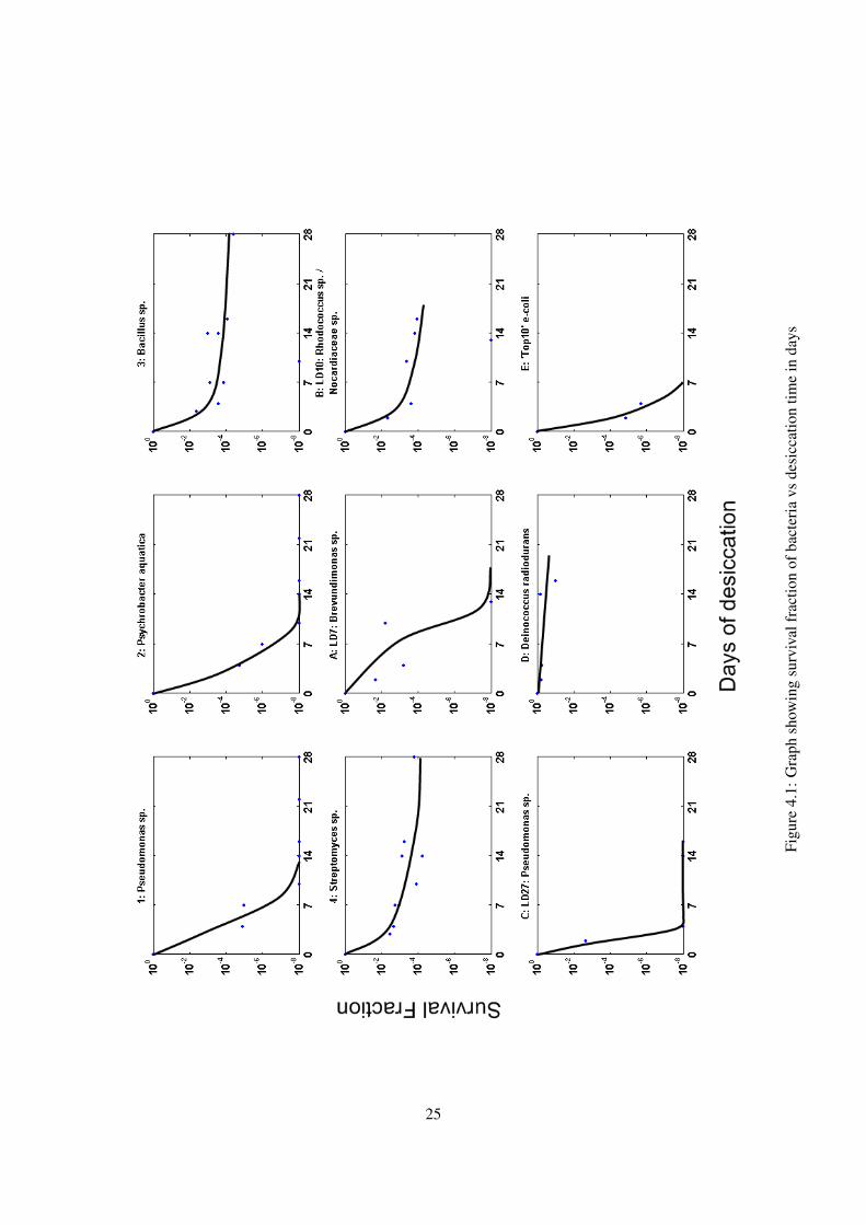
Figu

re4.

1:G

raph

show

ing

surv

ival

frac

tion

ofba

cter

iavs

desi

ccat

ion

time

inda

ys

25

4.2 UVC Resistance Results

The results for the UVC resistance experiments were highly chaotic and of low reliability and extremelylow repeatability. For this reason the results are not presented in this project.

Contamination (in the form of large apparently fungal growth on the agar plates) was a particularproblem and prevented a CFU count being obtained in approximately 50% of cases. The reason for suchhigh contamination was probably the large number of plates which were streaked with UVC exposedbacteria at zero dilution. This effectively measured the contaminant level of the cabinet which was, ifnot greater in frequency than the number of viable bacteria, at least faster growing than the bacteria, andtherefore dominated the agar plate.

26

Chapter 5

Discussion of Experimental Results

5.1 Desiccation Results

The graphs clearly show that D. radiodurans exhibits the greatest desiccation resistance of all the bac-teria tested, with survival several orders of magnitude better than the closest competitors. The Bacillussp., Streptomyces sp. and Rhodococcus sp./Nocardiaceae sp. all show intermediate desiccation resis-tance; all other bacteria exhibit relatively poor resistance and are essentially completely wiped out byone week of desiccation. The LD10 bacteria sample was found to be Pseudomonas sp., and although itdid not resemble the Pseudomonas sp. from the Miers Valley in appearance, the desiccation resistancewas similarly poor.

With the exception of the results for deinococcus, there is rather wide spread of data for all bacteria –for example the results for Bacillus sp. after 14 days has two data points, measured on separate occasionswith different samples. Although they look reasonably close on the graph, the scale is logarithmic andhides a significant difference of survival factor between the two samples. Worse still is an experimentat 10 days desiccation which showed near zero survival; probably this is an outlier, but it is also anindication that the experimental process does not give a high degree of repeatability.

The high variability may be due to different rates of desiccation depending on where the bacteriawas placed in the desiccator – high away from the desiccant, or immediately above it. Although thehumidity within the tub was assumed to be low and constant throughout, there is no way to guaranteethis with the equipment used. A possible improvement would be to use a specially designed desiccatorunit rather than the improvised Nalgene tubs.

The results for Breveundimonas sp. seem inconclusive - with only a few data points to draw upon, itis unclear whether the bacteria is killed completely after 14 days of desiccation, or whether that was ananomalous result, and that in fact the bacteria has resistance similar to that of the Streptomyces sp.

Overall the results are consistent with the hypothesis that those bacteria which are found in extremeenvironmental conditions display better resistance to desiccation than those from more moderate condi-tions. The Bacillus sp. (a spore forming bacteria) and Streptomyces sp. were Miers Valley bacteria foundin an exposed area, whereas as the Miers Valley Pseudomonas sp. and Psychrobacter aquaticus werefound sheltered by an algal mat, where they would not naturally experience such desiccating conditions.

There seems to be a general trend in the results where the initial desiccation process rapidly deci-mates the bacteria population; the difference in resistance across the bacterial strains seems to be thatthe weaker bacteria continue to die with continued time spent desiccated, whilst the survival rate of themore resistant bacteria reaches a plateau. It is possible that for the more resistant bacteria the desicca-tion provides a selection process, where the weaker members of the population die first leaving only thestronger members which are harder to kill, and which do not suffer from continued desiccation.

It is not possible to accurately calculate the ultimate survival time of the resistant bacteria fromthis data for continued desiccation as the curves drawn through the data are too arbitrary to support

27

extrapolation. However from the look of the results, it looks likely that the desiccation resistant bacteriawould remain viable above a one-in-a-million survival threshold for perhaps as long as two months,compared with just two weeks (at most) for the weaker bacteria. D. radiodurans seems to be remarkablyresilient and from the data gathered, would perhaps be able to survive above a one per million thresholdfor up to six months.

5.2 Comparison of Desiccation Resistance and γ-Radiation Resistance

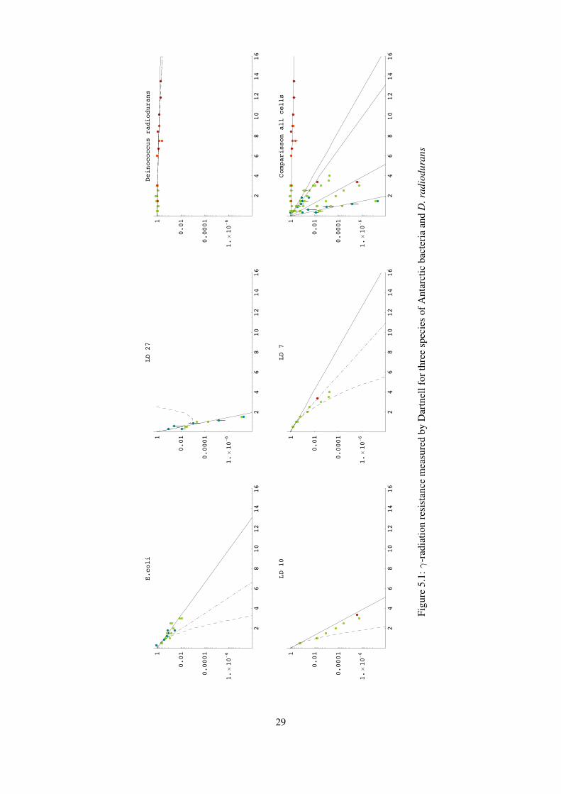
Figure 5.1 (provided by Dartnell) shows γ-radiation resistance for the bacteria e. coli, LD7, LD10,LD27 (Brevundimonas sp., Rhodococcus sp./Nocardiaceae sp., Pseudomonas sp. respectively) and D.radiodurans. Neglecting e. coli, the qualitative correspondence between this graph and the desiccationresults is striking, and supports the hypothesis that desiccation resistance is a good indicator of radiationresistance. In fact desiccation, which induces DNA double strand breaks, seems more harmful to D.radiodurans than relatively high doses of γ-radiation, which is after all only weakly ionizing. Thissuggests that either the desiccation regime produced more double strand breaks than the γ radiationexposure, or that another form of biological damage is also occuring to kill the bacteria.

28

24

68

10

12

14

16

1.!10"6

0.0001

0.011

LD10

24

68

10

12

14

16

1.!10"6

0.0001

0.011

LD7

24

68

10

12

14

16

1.!10"6

0.0001

0.011

Comparissonallcells

24

68

10

12

14

16

1.!10"6

0.0001

0.011

E.coli

24

68

10

12

14

16

1.!10"6

0.0001

0.011

LD27

24

68

10

12

14

16

1.!10"6

0.0001

0.011

Deinococcusradiodurans

Figu

re5.

1:γ

-rad

iatio

nre

sist

ance

mea

sure

dby

Dar

tnel

lfor

thre

esp

ecie

sof

Ant

arct

icba

cter

iaan

dD

.rad

iodu

rans

29

Dartnell suggests that the strangely high radiation resistance for e. coli is an artifact of the experi-mental process, which in fact kills 99% of the e. coli by freezing before they are irradiated, leading toartificially high rates of survival of the remaining, extra-resilient, bacteria.

Although the data collected for this project is insufficient to calculate a direct “exchange rate” be-tween desiccation exposure and γ-radiation irradiation, the principle seems reasonable, and with furtherdata points to provide greater resolution of the graphs in Figure 4.1, such a comparison could be made.

5.3 UVC Radiation Resistance

The lack of results for UVC radiation resistance were probably insufficient sterlisation of the cabinetbefore use (overnight sterlisation seems to be required rather than just a few hours), and shielding of thebacteria by the edges of the petri dishes. In addition it is possible that the UVC source is in fact veryintense, but is unable to penetrate any depth at all of the liquid broth, leading to self-shielding even of theextremely thin layer. Consequently aliquots taken for testing would incorporate a mixture of irradiatedand shielded material, giving spurious results.

An Improved UVC Protocol?

In order to improve upon the results yielded by the UVC protocol outlined in Section 3.4, a secondprotocol was tried where instead of 500µl samples in petri dishes, a ’dot matrix’ of 10µl aliquots wasplaced on a 90mm petri dish, deliberately taking advantage of the high surface tension to give stablehemispheres of liquid on the surface.

After exposure, a single ’dot’ could be collected in its entirety and diluted as appropriate. Theadvantages of this protocol are:

• Definite similarity of UVC exposure between all ’dots’ since they are identical

• No ’shadowing’ from the sides of the dish

• No tendency for liquid to collect in the edges of the dish due to convexity of the dish surface

• Virtually 100% recovery of exposed material since the entire 10µl dot can be pipetted back afterexposure

The main disadvantages are that the dot will inevitably self-shield so that bacteria in the centre ofthe dot are protected, and there is an increased risk of contamination from spores in the cabinet whichwere not destroyed by the pre-sterilising process.

It is difficult to assess the performance of the second protocol since time constraints on the projectlimited its use to a single set of experiments, where 5 bacteria samples and one control dish (containingdots of nutrient broth) were irradiated for 5, 12, and 30 minutes. The contamination level of the resultswas found to be high, with fungal-type growth dominating three of the agar plates produced. The otherproblem was a lack of positive results – the CFU count for almost all of the plates was zero, except forD. radiodurans which at 30 minutes exposure produced a CFU count higher than that for 12 minutesexposure. Similarly the LD27 Pseudomonas sp. produced a CFU count at 30 minutes, but not after 12minutes.

In summary the second protocol did not appear to perform any better than the original protocol,again due to both insufficient sterilisation of the cabinet before use, and self-shielding of the bacteria.

Another possible solution is to irradiate a desiccated sample of bacteria, in a combined desiccationplus UVC regime. However the variability evident in the results for the desiccation experiments couldwell obscure any effect of UVC exposure.

30

Chapter 6

Further Work

The simulation/modelling component of this project is tantalisingly close to producing significant results– a complete LET spectrum for the Martian surface under the impact of both SEP and GCR for particlesup to 1 TeV energy. A little more computer simulation and time to post-process, and re-validate theresults is all that is required, although the rogue γ radiation registering high LET needs to be resolved. Inaddition the results offer a wide variety of avenues to explore: linking the LET spectrum to a desiccationregime for bacteria to estimate survival times of sub-surface bacteria is still a plausible possibility;assembling a ’best-fit’ LET spectrum to simulate that of Mars using lab-ready radio-nuclide sources.

The desiccation experiments in this project could be extended by repeating the experiments alreadyperformed to provide more statistical basis for the results, and to hopefully reduce the variability ob-served so far. Once data is obtained through which a survival curve can be accurately fitted, a directcorrelation with γ resistance may be possible. In addition it may be desirable to use an industrial-typefreeze-drying method for desiccation to more accurately model the conditions found on Mars, ratherthan the slow and presumably more gentle bench-top desiccation method followed here. In additionit would be advisable to repeat the experiments using bacteria cultured at low temperature rather thanroom temperature to check for variation in gene expression with growing conditions.

The UVC resistance experiments could be tried with an alternative UV source, e.g. hand-held lamp.Although this was available for use during this project, the cabinet was selected for convenience since itwas believed to provide a more constant experimental environment, and was simpler to set up. Howeverthe protocols used in this project failed to produce any results, so other avenues should be explored.

31

Chapter 7

Acknowledgements

I would like to acknowledge the help and encouragement I received from my supervisors. I would alsolike to thank Lewis Dartnell, upon who’s PhD work this project is based, for his support and encourage-ment.

32

Bibliography

[1] David J. Stevenson. Mars’ core and magnetism. Nature, 412(6843), 2001.

[2] Brad Lobitz, Byron L. Wood, Maurice M. Averner, and Christopher P. McKay. Special feature:Use of spacecraft data to derive regions on mars where liquid water would be stable. PNAS, 98(5),2001.

[3] Philippe Masson, Michael H. Carr, Franois Costard, Ronald Greeley, Ernst Hauber, and Ralf Jau-mann. Geomorphologic evidence for liquid water. Space Science Reviews, 96(1-4), 2001.

[4] R. L. Mancinelli and A. Banin. Life on mars? ii. physical restrictions. Advances in Space Research,15(3), 1995.

[5] David A. Brain and Bruce M. Jakosky. Atmospheric loss since the onset of the martian geologicrecord: Combined role of impact erosion and sputtering. Journal of Geophysical Research, 103,1998.

[6] C Horneck, G; Baumstark-Khan, editor. Astrobiology: The Quest for the Conditions of Life.Springer, 2001.

[7] L. R. Dartnell, L. Desorgher, J. M. Ward, and A. J. Coates. Martian sub-surface ionising radiation:biosignatures and geology. Biogeosciences Discussions, 4:455–492, February 2007.

[8] S. Agostinelli and others. Geant4 — a simulation toolkit. Nuclear Instruments and Methods inPhysics Research, A(506):250–303, 2003.

[9] Laurent Desorgher, E. O. FLCKIGER, M. Gurtner, M.R. Moser, and R. BTIKOFER. Atmocos-mics: A geant 4 code for computing the interaction of cosmic rays with the earth’s atmosphere.International Journal of Modern Physics A (IJMPA), 20:6802 – 6804, 2005.

[10] L.R. Dartnell, L. Desorgher, J.M. Ward, and A.J. Coates. Modelling the surface and subsurfacemartian radiation environment: Implications for astrobiology. Geophys. Res. Lett., 2007.

[11] John W. Wilson and Francis F. Badawi. A study of the generation of linear energy transfer specrafor space radiations.

[12] F. Cucinotta, J. Wilson, J. Shinn, F. Badavi, and G. Badhwar. Effects of target fragmentation onevaluation of let spectra from space radiation: Implications for space radiation protection studies,1996.

[13] M. T. La Duc, J. N. Benardini, M. J. Kempf, D. A. Newcombe, M. Lubarsky, andK. Venkateswaran. Microbial Diversity of Indian Ocean Hydrothermal Vent Plumes: Microbes Tol-erant of Desiccation, Peroxide Exposure, and Ultraviolet and γ-Irradiation. Astrobiology, 7:416–431, May 2007.

33

[14] Samantha Whiting. Investigation of Genome Diversity in Antarctic Dry Valley Soils. PhD thesis,UCL, 2004.

34