modelling construction phasesofboredtunnels
TRANSCRIPT

Modelling constructionphases of bored tunnelswith respect to internallining forcesA comparison of Finite ElementProgramsD.J. Kunst


Modelling construction phases ofbored tunnels with respect to
internal lining forcesA comparison of Finite Element Programs
by
D.J. Kunstto obtain the degree of Master of Science
at the Delft University of Technology,
Student number: 4135393Project duration: October 1, 2016 – July 19, 2017Thesis committee: Dr. ir. W. Broere, TU Delft, chairman
Dr. P. J. Vardon, TU DelftDr. ir. C. B. M. Blom, TU DelftIr. B. Safari, Arthe Civil and Structure bv


Preface
Before you lies the thesis "Modelling construction phases of bored tunnels with respect to internal liningforces: A comparison of finite element programs".
This will be the final document in completion of the master programme Geo-Engineering at Delft univer-sity of Technology. I have worked on the research and writing from October 2016 until July 2017.
Together with Arthe Civil and Structure I have found this interesting topic in which much was to learnfor both parties. It proved to be more difficult than initially expected. Days of battelling with the computerprograms, only to come as winner occasionally. Fortunately, with some dedication and mostly perseverance Ihave been able to win a sufficient amount of times in order to answer the determined question. The sparringand joined modelling sessions together with Mr. Liem have really helped in understanding the issues andfinding correct solutions. His input has helped shape this thesis.
I would like to thank Messrs. Hoffmann and Partovi of DIANA for their support with the program. Withtheir help, I managed to create the models I could not do without in this research.
Furthermore I would like to thank Mr. Safari and my other committee members whose input during ourmeetings was very welcome. My other colleagues at Arthe CS have made sure I saw the humorous side ofsome of my situations, which I am them thankful for.
Last but not least, I would like to thank my parents, girlfriend and friends for the motivational words everynow and then. It has helped me through tough times.
Please, enjoy your reading.
D.J. KunstDelft, July 2017
iii


Abstract
Areas are getting more and more populated causing new infrastructure lines to be constructed below thesurface. A bored tunnel is one of the possibilities to create this subsurface infrastructure, but the constructionprocess of a bored tunnel is a complicated one. Many loads and aspects are present in this constructionprocess that can be divided into six phases. In each of these phases, different loads and aspects are acting onthe tunnel lining or the surrounding soil which can cause the lining to deform.
The increasing complexity and demands of problems have led to the use of the finite element method. Acomputer based method which allows one to model the problem.
For finite element modelling, numerous programs are available of which several claim to be able to modelbored tunnels. However, it is not yet clear what the exact differences between the different programs are. Withmany aspects to be modelled, many differences between programs occur, either in the soil, the tunnel liningor a combination of both.
This research has focussed on the possibilities of modelling the different construction phases of boredtunnels in two widely used programs: DIANA and Plaxis. Simple two dimensional (2D) models were cre-ated to which the different construction phases were added before continuing with three dimensional (3D)modelling. This approach has led to a good assessment of the possibilities and limitations within these twoprograms.
DIANA is not yet suitable for modelling the construction process of bored tunnels completely. The con-struction phases are modelled undrained to account for the relative short time they are acting. A consoli-dation phase in which the pore pressure can dissipate cannot be modelled in DIANA, which is essential formodelling the construction phases.
Plaxis, on the contrary, is not able to model joints in the segmental lining appropriate for 3D. In 3D, Plaxisonly allows to model a joints as "fixed" or "free". In DIANA different theories can be applied to the joints,including Janssens. For 2D, both programs have a rotational springs besides the free and fixed connection formodelling the joints.
For the model in which the material models were changed, the difference with the main impact betweenthe two programs occurred, especially for the bending moment. This means the Modified Mohr-Colombmaterial model in DIANA is different than the Hardening Soil model in Plaxis.
Including the construction phases leads to more favourable internal lining forces for tunnels, somethingof which clients should be convinced. However, not until the models have been benchmarked with measureddata from a tunnel project.
While 3D models have been investigated in this research, they should be extended in order have a betterunderstanding of the different 3D phenomena that are present in the construction of bored tunnels. This willboth assess the possibilities of modelling this process and more potential differences between programs canbe investigated.
Besides extending the 3D models, other programs should be investigated on their capabilities too. Inorder to come to a proper assessment of the possibilities, program experience is strongly recommended.These programs should also be compared with measured data for benchmark purposes.
v


Contents
Preface . . . . . . . . . . . . . . . . . . . . . . . . . . . . . . . . . . . . . . . . . . . . . . . . . iiiAbstract . . . . . . . . . . . . . . . . . . . . . . . . . . . . . . . . . . . . . . . . . . . . . . . . v
List of Figures xi
List of Tables xv
1 Introduction 11.1 Problem Description . . . . . . . . . . . . . . . . . . . . . . . . . . . . . . . . . . . . . . . 21.2 Research Questions . . . . . . . . . . . . . . . . . . . . . . . . . . . . . . . . . . . . . . . . 2
2 Literature Review 52.1 Design procedure . . . . . . . . . . . . . . . . . . . . . . . . . . . . . . . . . . . . . . . . . 52.2 Loads, forces and deformations . . . . . . . . . . . . . . . . . . . . . . . . . . . . . . . . . . 6
2.2.1 Construction phases . . . . . . . . . . . . . . . . . . . . . . . . . . . . . . . . . . . . 82.2.2 Loads during construction phases . . . . . . . . . . . . . . . . . . . . . . . . . . . . . 92.2.3 Lining deformations . . . . . . . . . . . . . . . . . . . . . . . . . . . . . . . . . . . . 112.2.4 Slip or bonded ground-lining interaction . . . . . . . . . . . . . . . . . . . . . . . . . 12
2.3 Tunnel lining design . . . . . . . . . . . . . . . . . . . . . . . . . . . . . . . . . . . . . . . 122.3.1 Schulze-Duddeck method . . . . . . . . . . . . . . . . . . . . . . . . . . . . . . . . . 122.3.2 Ring action. . . . . . . . . . . . . . . . . . . . . . . . . . . . . . . . . . . . . . . . . 132.3.3 Beam action . . . . . . . . . . . . . . . . . . . . . . . . . . . . . . . . . . . . . . . . 132.3.4 Joints. . . . . . . . . . . . . . . . . . . . . . . . . . . . . . . . . . . . . . . . . . . . 15
2.4 Finite Element Method Programs . . . . . . . . . . . . . . . . . . . . . . . . . . . . . . . . . 182.4.1 Plaxis . . . . . . . . . . . . . . . . . . . . . . . . . . . . . . . . . . . . . . . . . . . 182.4.2 DIANA . . . . . . . . . . . . . . . . . . . . . . . . . . . . . . . . . . . . . . . . . . . 192.4.3 CESAR-LCPC. . . . . . . . . . . . . . . . . . . . . . . . . . . . . . . . . . . . . . . . 192.4.4 GTS NX . . . . . . . . . . . . . . . . . . . . . . . . . . . . . . . . . . . . . . . . . . 192.4.5 Other . . . . . . . . . . . . . . . . . . . . . . . . . . . . . . . . . . . . . . . . . . . 192.4.6 Conclusion. . . . . . . . . . . . . . . . . . . . . . . . . . . . . . . . . . . . . . . . . 20
2.5 Parametric studies . . . . . . . . . . . . . . . . . . . . . . . . . . . . . . . . . . . . . . . . 202.5.1 Soil parameters . . . . . . . . . . . . . . . . . . . . . . . . . . . . . . . . . . . . . . 202.5.2 Tunnel parameters . . . . . . . . . . . . . . . . . . . . . . . . . . . . . . . . . . . . . 222.5.3 Lining parameters . . . . . . . . . . . . . . . . . . . . . . . . . . . . . . . . . . . . . 23
2.6 Soil models . . . . . . . . . . . . . . . . . . . . . . . . . . . . . . . . . . . . . . . . . . . . 232.6.1 Mohr-Coulomb . . . . . . . . . . . . . . . . . . . . . . . . . . . . . . . . . . . . . . 242.6.2 Hardening Soil . . . . . . . . . . . . . . . . . . . . . . . . . . . . . . . . . . . . . . . 242.6.3 Hardening Soil small strain . . . . . . . . . . . . . . . . . . . . . . . . . . . . . . . . 252.6.4 (Modified) Cam-Clay. . . . . . . . . . . . . . . . . . . . . . . . . . . . . . . . . . . . 252.6.5 Concluding remarks . . . . . . . . . . . . . . . . . . . . . . . . . . . . . . . . . . . . 26
2.7 Concrete models . . . . . . . . . . . . . . . . . . . . . . . . . . . . . . . . . . . . . . . . . 272.8 Ground-lining interaction methods . . . . . . . . . . . . . . . . . . . . . . . . . . . . . . . . 27
2.8.1 Grouting pressure . . . . . . . . . . . . . . . . . . . . . . . . . . . . . . . . . . . . . 272.8.2 Concluding remarks . . . . . . . . . . . . . . . . . . . . . . . . . . . . . . . . . . . . 29
2.9 Final model properties . . . . . . . . . . . . . . . . . . . . . . . . . . . . . . . . . . . . . . 29
3 Methodology 333.1 Different models . . . . . . . . . . . . . . . . . . . . . . . . . . . . . . . . . . . . . . . . . 33
3.1.1 2-Dimensional . . . . . . . . . . . . . . . . . . . . . . . . . . . . . . . . . . . . . . . 333.1.2 3-Dimensional . . . . . . . . . . . . . . . . . . . . . . . . . . . . . . . . . . . . . . . 37
vii
viii Contents
3.2 2D modelling techniques . . . . . . . . . . . . . . . . . . . . . . . . . . . . . . . . . . . . . 383.2.1 Plaxis . . . . . . . . . . . . . . . . . . . . . . . . . . . . . . . . . . . . . . . . . . . 383.2.2 Modelling in DIANA . . . . . . . . . . . . . . . . . . . . . . . . . . . . . . . . . . . . 40
3.3 3D modelling techniques . . . . . . . . . . . . . . . . . . . . . . . . . . . . . . . . . . . . . 423.3.1 Plaxis . . . . . . . . . . . . . . . . . . . . . . . . . . . . . . . . . . . . . . . . . . . 423.3.2 DIANA . . . . . . . . . . . . . . . . . . . . . . . . . . . . . . . . . . . . . . . . . . . 43
4 Results 454.1 2-Dimensional . . . . . . . . . . . . . . . . . . . . . . . . . . . . . . . . . . . . . . . . . . 45
4.1.1 Model One . . . . . . . . . . . . . . . . . . . . . . . . . . . . . . . . . . . . . . . . . 454.1.2 Model Two . . . . . . . . . . . . . . . . . . . . . . . . . . . . . . . . . . . . . . . . . 454.1.3 Model Three . . . . . . . . . . . . . . . . . . . . . . . . . . . . . . . . . . . . . . . . 464.1.4 Model Four . . . . . . . . . . . . . . . . . . . . . . . . . . . . . . . . . . . . . . . . 474.1.5 Model Five . . . . . . . . . . . . . . . . . . . . . . . . . . . . . . . . . . . . . . . . . 484.1.6 Model Six . . . . . . . . . . . . . . . . . . . . . . . . . . . . . . . . . . . . . . . . . 484.1.7 Model Seven . . . . . . . . . . . . . . . . . . . . . . . . . . . . . . . . . . . . . . . . 494.1.8 Model Eight . . . . . . . . . . . . . . . . . . . . . . . . . . . . . . . . . . . . . . . . 494.1.9 Model Nine . . . . . . . . . . . . . . . . . . . . . . . . . . . . . . . . . . . . . . . . 514.1.10 Development throughout construction process . . . . . . . . . . . . . . . . . . . . . . 514.1.11 Model Ten . . . . . . . . . . . . . . . . . . . . . . . . . . . . . . . . . . . . . . . . . 534.1.12 Model Eleven . . . . . . . . . . . . . . . . . . . . . . . . . . . . . . . . . . . . . . . 534.1.13 Model Twelve . . . . . . . . . . . . . . . . . . . . . . . . . . . . . . . . . . . . . . . 54
4.2 3-Dimensional . . . . . . . . . . . . . . . . . . . . . . . . . . . . . . . . . . . . . . . . . . 554.2.1 One-ring models . . . . . . . . . . . . . . . . . . . . . . . . . . . . . . . . . . . . . . 554.2.2 Without construction phases . . . . . . . . . . . . . . . . . . . . . . . . . . . . . . . 554.2.3 With construction phases . . . . . . . . . . . . . . . . . . . . . . . . . . . . . . . . . 56
5 Discussion 575.1 2-Dimensional . . . . . . . . . . . . . . . . . . . . . . . . . . . . . . . . . . . . . . . . . . 57
5.1.1 Model One . . . . . . . . . . . . . . . . . . . . . . . . . . . . . . . . . . . . . . . . . 575.1.2 Model Two . . . . . . . . . . . . . . . . . . . . . . . . . . . . . . . . . . . . . . . . . 575.1.3 Interface sensitivity . . . . . . . . . . . . . . . . . . . . . . . . . . . . . . . . . . . . 575.1.4 Model Three . . . . . . . . . . . . . . . . . . . . . . . . . . . . . . . . . . . . . . . . 595.1.5 Model Four . . . . . . . . . . . . . . . . . . . . . . . . . . . . . . . . . . . . . . . . 615.1.6 Mohr-Coulomb vs Hardening Soil . . . . . . . . . . . . . . . . . . . . . . . . . . . . . 615.1.7 Model Five . . . . . . . . . . . . . . . . . . . . . . . . . . . . . . . . . . . . . . . . . 635.1.8 Hardened grout stiffness sensitivity . . . . . . . . . . . . . . . . . . . . . . . . . . . . 645.1.9 Model Six . . . . . . . . . . . . . . . . . . . . . . . . . . . . . . . . . . . . . . . . . 645.1.10 Model Seven . . . . . . . . . . . . . . . . . . . . . . . . . . . . . . . . . . . . . . . . 675.1.11 Grout pressure increment sensitivity. . . . . . . . . . . . . . . . . . . . . . . . . . . . 685.1.12 Model Eight . . . . . . . . . . . . . . . . . . . . . . . . . . . . . . . . . . . . . . . . 685.1.13 Model Nine . . . . . . . . . . . . . . . . . . . . . . . . . . . . . . . . . . . . . . . . 695.1.14 Model Ten . . . . . . . . . . . . . . . . . . . . . . . . . . . . . . . . . . . . . . . . . 705.1.15 Model Eleven . . . . . . . . . . . . . . . . . . . . . . . . . . . . . . . . . . . . . . . 715.1.16 Model Twelve . . . . . . . . . . . . . . . . . . . . . . . . . . . . . . . . . . . . . . . 715.1.17 Last models . . . . . . . . . . . . . . . . . . . . . . . . . . . . . . . . . . . . . . . . 71
5.2 3-Dimensional . . . . . . . . . . . . . . . . . . . . . . . . . . . . . . . . . . . . . . . . . . 725.2.1 One-ring models . . . . . . . . . . . . . . . . . . . . . . . . . . . . . . . . . . . . . . 725.2.2 Without construction phases . . . . . . . . . . . . . . . . . . . . . . . . . . . . . . . 735.2.3 With construction phases . . . . . . . . . . . . . . . . . . . . . . . . . . . . . . . . . 74
6 Conclusion 777 Recommendations 79Bibliography 83A Schematic overviewmodelling 87B Model overview 89

Contents ix
C Finite elementmodels 91C.1 General information . . . . . . . . . . . . . . . . . . . . . . . . . . . . . . . . . . . . . . . 91C.2 Input . . . . . . . . . . . . . . . . . . . . . . . . . . . . . . . . . . . . . . . . . . . . . . . 91
D Analytical validation 99E Interface sensitivity graphs 103F Total displacements around tunnel 109G Hardened grout stiffness sensitivity 113H MN-kappa diagrams 2D 117
H.1 Plaxis . . . . . . . . . . . . . . . . . . . . . . . . . . . . . . . . . . . . . . . . . . . . . . . 118H.2 DIANA . . . . . . . . . . . . . . . . . . . . . . . . . . . . . . . . . . . . . . . . . . . . . . 123
I One-ringmodels comparison 127


List of Figures
1.1 Constructed tunnel where the tunnel lining is still clearly visible [39]. . . . . . . . . . . . . . . . . 1
2.1 Three different ways to evaluate ground pressure load acting on tunnel lining [42]. . . . . . . . . 62.2 Water pressure load acting on tunnel lining [42]. . . . . . . . . . . . . . . . . . . . . . . . . . . . . . 72.3 Vertical subgrade reaction on the tunnel lining [42]. . . . . . . . . . . . . . . . . . . . . . . . . . . 72.4 The first five construction phases distinguished by Bakker [4], the sixth phase is long term effects. 92.5 The five construction phases determined by Mair and Taylor [60] after Cording [25]. . . . . . . . 92.6 Ovalisation load (a) and the deformation caused by this load (b). . . . . . . . . . . . . . . . . . . . 112.7 Two types of buckling deformation of tunnel lining [18]. . . . . . . . . . . . . . . . . . . . . . . . . 122.8 A spring model (a) and a continuum model (b) for radial action [58]. . . . . . . . . . . . . . . . . . 142.9 Bending of the tunnel lining (a) and a simplified one-dimensional model of beam action (b) [58] 142.10 A bending beam (a) and a shear beam (b) [10] . . . . . . . . . . . . . . . . . . . . . . . . . . . . . . 152.11 Definition of circumferential and longitudinal joint [24]. . . . . . . . . . . . . . . . . . . . . . . . . 162.12 Five connection systems for construction of segmental tunnel lining. . . . . . . . . . . . . . . . . 172.13 Stiffness-strain behaviour of soil. Strain ranges for different structures have been indicated as
well [12]. . . . . . . . . . . . . . . . . . . . . . . . . . . . . . . . . . . . . . . . . . . . . . . . . . . . . 25
3.1 Close up of the two phases in the "Mohr-Coulomb One Layer" model . . . . . . . . . . . . . . . . 333.2 Close up of the two phases in the "Mohr-Coulomb Eight Layers" model . . . . . . . . . . . . . . . 343.4 The lining with the locations of the joints . . . . . . . . . . . . . . . . . . . . . . . . . . . . . . . . . 353.3 Close-up schematisation for the different phases that will be applied in the models . . . . . . . . 363.5 Overview of the model with buildings . . . . . . . . . . . . . . . . . . . . . . . . . . . . . . . . . . . 373.6 Manual Janssen iteration procedure . . . . . . . . . . . . . . . . . . . . . . . . . . . . . . . . . . . . 40
4.1 Phases in model one . . . . . . . . . . . . . . . . . . . . . . . . . . . . . . . . . . . . . . . . . . . . . 454.3 Phases in model two . . . . . . . . . . . . . . . . . . . . . . . . . . . . . . . . . . . . . . . . . . . . . 454.2 Results for the normal force and bending moment for model one . . . . . . . . . . . . . . . . . . 464.4 Results for the normal force and bending moment for model two. . . . . . . . . . . . . . . . . . . 464.5 Results for the normal force and bending moment for model three . . . . . . . . . . . . . . . . . . 474.6 Results for the normal force and bending moment for model four . . . . . . . . . . . . . . . . . . 474.7 Phases in model five . . . . . . . . . . . . . . . . . . . . . . . . . . . . . . . . . . . . . . . . . . . . . 484.8 Results for the normal force and bending moment for model five . . . . . . . . . . . . . . . . . . . 484.9 Phases in model six . . . . . . . . . . . . . . . . . . . . . . . . . . . . . . . . . . . . . . . . . . . . . . 484.10 Results for the normal force and bending moment for model six . . . . . . . . . . . . . . . . . . . 494.11 Phases in model seven . . . . . . . . . . . . . . . . . . . . . . . . . . . . . . . . . . . . . . . . . . . . 494.14 Phases in model eight . . . . . . . . . . . . . . . . . . . . . . . . . . . . . . . . . . . . . . . . . . . . 494.12 Results for the normal force and bending moment for model seven . . . . . . . . . . . . . . . . . 504.13 Results for the normal force and bending moment for undrained model seven . . . . . . . . . . . 504.15 Results for the normal force and bending moment for undrained model eight . . . . . . . . . . . 514.16 Phases in model nine . . . . . . . . . . . . . . . . . . . . . . . . . . . . . . . . . . . . . . . . . . . . . 514.17 Results for the normal force and bending moment for model nine . . . . . . . . . . . . . . . . . . 524.18 Development of the internal lining forces over the complete construction process . . . . . . . . 524.19 Ratio and absolute difference between Plaxis and DIANA . . . . . . . . . . . . . . . . . . . . . . . 534.20 Lining forces for Hardening Soil and Mohr Coulomb material models for models five to nine . . 534.21 Joint numbering and accompanying rotational stiffness . . . . . . . . . . . . . . . . . . . . . . . . 544.22 Results for the normal force and bending moment for model eleven . . . . . . . . . . . . . . . . . 544.23 Results for the normal force and bending moment for model twelve . . . . . . . . . . . . . . . . . 554.24 Development of the internal lining forces over the different models in 2D and 3D . . . . . . . . . 554.25 The internal lining forces for the multiple ring models without construction phases . . . . . . . 56
xi

xii List of Figures
4.26 The internal lining forces for the two and three dimensional models with the construction phases. 56
5.1 Lining forces for different reduction factors on interface strength in Plaxis and DIANA . . . . . . 585.2 Lining forces for different reduction factors on interface strength for different multiplication
factors in DIANA . . . . . . . . . . . . . . . . . . . . . . . . . . . . . . . . . . . . . . . . . . . . . . . 585.3 Interface stresses for different values of the reduction factor in Plaxis . . . . . . . . . . . . . . . . 595.4 Interface stresses for different values of the reduction factor in DIANA . . . . . . . . . . . . . . . 595.5 Lining forces for different reduction factors with the same input for the interface strength . . . . 605.6 Total displacements for model four in Plaxis and DIANA . . . . . . . . . . . . . . . . . . . . . . . . 615.7 Results for the normal force and bending moment for model four with full bonding . . . . . . . 625.8 Results for the normal force and bending moment for the Mohr-Coulomb and Hardening Soil
material models in Plaxis . . . . . . . . . . . . . . . . . . . . . . . . . . . . . . . . . . . . . . . . . . 625.9 Results for the normal force and bending moment for the Mohr-Coulomb and Hardening Soil
material models in DIANA . . . . . . . . . . . . . . . . . . . . . . . . . . . . . . . . . . . . . . . . . . 635.10 Phase displacement in phase with TBM . . . . . . . . . . . . . . . . . . . . . . . . . . . . . . . . . . 645.11 Lining forces for different values of the hardened grout stiffness . . . . . . . . . . . . . . . . . . . 645.12 Phase displacement in the taper phase for contraction in Plaxis and prescribed deformation in
DIANA . . . . . . . . . . . . . . . . . . . . . . . . . . . . . . . . . . . . . . . . . . . . . . . . . . . . . 655.13 Phase displacement in the taper phase for stress release in Plaxis and DIANA . . . . . . . . . . . 655.14 Lining forces for different values of the stress release . . . . . . . . . . . . . . . . . . . . . . . . . . 665.15 Displacement for top and bottom of the borehole for different stress releases . . . . . . . . . . . 665.16 Exaggeration of possible TBM behaviour in borehole . . . . . . . . . . . . . . . . . . . . . . . . . . 675.17 Lining forces for drained and undrained analysis in Plaxis for different models . . . . . . . . . . . 675.18 Lining forces for different values of the vertical grout pressure gradient . . . . . . . . . . . . . . . 685.19 Results for the normal force and bending moment for two follow cart modelling approaches . . 695.20 Extreme lining force values for different values of the inlay stiffness . . . . . . . . . . . . . . . . . 695.21 Lining forces in the tunnel lining for different values of the inlay stiffness . . . . . . . . . . . . . . 705.22 Phase displacement in the grouting phase for Hardening Soil and Mohr-Coulomb material mod-
els in Plaxis . . . . . . . . . . . . . . . . . . . . . . . . . . . . . . . . . . . . . . . . . . . . . . . . . . . 715.23 Extreme lining force values for models seven to twelve . . . . . . . . . . . . . . . . . . . . . . . . . 715.24 Unity check for all the models in 2D . . . . . . . . . . . . . . . . . . . . . . . . . . . . . . . . . . . . 725.25 The internal lining forces for model four and the 3D model in DIANA . . . . . . . . . . . . . . . . 735.26 The internal lining forces for model four and the 3D model in Plaxis . . . . . . . . . . . . . . . . . 745.27 Internal lining force for the 10 ring model with construction phases in Plaxis . . . . . . . . . . . . 745.28 Bending moments in the longitudinal direction for newly installed rings with normally fixed (a)
and fully fixed (b) front of the model . . . . . . . . . . . . . . . . . . . . . . . . . . . . . . . . . . . . 755.29 Internal lining forces for the 10 ring model with construction phases in Plaxis with complete
fixation at front of the model . . . . . . . . . . . . . . . . . . . . . . . . . . . . . . . . . . . . . . . . 755.30 Lining forces for the front, middle and back of a ring in the 3D ring model with construction
phases . . . . . . . . . . . . . . . . . . . . . . . . . . . . . . . . . . . . . . . . . . . . . . . . . . . . . 76
B.1 Phases in model one . . . . . . . . . . . . . . . . . . . . . . . . . . . . . . . . . . . . . . . . . . . . . 89B.2 Phases in model two . . . . . . . . . . . . . . . . . . . . . . . . . . . . . . . . . . . . . . . . . . . . . 89B.3 Phases in model five . . . . . . . . . . . . . . . . . . . . . . . . . . . . . . . . . . . . . . . . . . . . . 89B.4 Phases in model six . . . . . . . . . . . . . . . . . . . . . . . . . . . . . . . . . . . . . . . . . . . . . . 89B.5 Phases in model seven . . . . . . . . . . . . . . . . . . . . . . . . . . . . . . . . . . . . . . . . . . . . 90B.6 Phases in model eight . . . . . . . . . . . . . . . . . . . . . . . . . . . . . . . . . . . . . . . . . . . . 90B.7 Phases in model nine . . . . . . . . . . . . . . . . . . . . . . . . . . . . . . . . . . . . . . . . . . . . . 90B.8 One-ring 3D model . . . . . . . . . . . . . . . . . . . . . . . . . . . . . . . . . . . . . . . . . . . . . . 90
C.1 Gradation of soil layer boundaries in meters in DIANA. . . . . . . . . . . . . . . . . . . . . . . . . . 93C.2 Mesh and supports of 2D Plaxis model . . . . . . . . . . . . . . . . . . . . . . . . . . . . . . . . . . 95C.3 Mesh and supports of 2D DIANA model . . . . . . . . . . . . . . . . . . . . . . . . . . . . . . . . . . 95C.4 Mesh of 3D Plaxis model . . . . . . . . . . . . . . . . . . . . . . . . . . . . . . . . . . . . . . . . . . . 96C.5 Mesh 3D DIANA model . . . . . . . . . . . . . . . . . . . . . . . . . . . . . . . . . . . . . . . . . . . 96C.6 Supports of 3D Plaxis model . . . . . . . . . . . . . . . . . . . . . . . . . . . . . . . . . . . . . . . . . 97C.7 Supports of 3D DIANA model . . . . . . . . . . . . . . . . . . . . . . . . . . . . . . . . . . . . . . . . 97

List of Figures xiii
E.1 Internal lining force results regarding the influence of the interface in Plaxis . . . . . . . . . . . . 103E.2 Internal lining force results regarding the influence of the interface in DIANA . . . . . . . . . . . 104E.3 Internal lining force results regarding the influence of multiplication factor for the interface
strength in DIANA . . . . . . . . . . . . . . . . . . . . . . . . . . . . . . . . . . . . . . . . . . . . . . 105E.4 Internal lining force results regarding the influence of the interface in Plaxis and DIANA . . . . . 106E.5 Results for the normal force and bending moment regarding the influence of the interface with
the same strength input parameters . . . . . . . . . . . . . . . . . . . . . . . . . . . . . . . . . . . . 107
F.1 Total displacements for model three in Plaxis and DIANA . . . . . . . . . . . . . . . . . . . . . . . 109F.2 Total displacements for model four in Plaxis and DIANA . . . . . . . . . . . . . . . . . . . . . . . . 109F.3 Total displacements for model five in Plaxis and DIANA . . . . . . . . . . . . . . . . . . . . . . . . 110F.4 Total displacements for model six in Plaxis and DIANA . . . . . . . . . . . . . . . . . . . . . . . . . 110F.5 Total displacements for model seven in Plaxis . . . . . . . . . . . . . . . . . . . . . . . . . . . . . . 110F.6 Total displacements for model nine in Plaxis . . . . . . . . . . . . . . . . . . . . . . . . . . . . . . . 111F.7 Total displacements for front of 3D model without construction phases . . . . . . . . . . . . . . . 111F.8 Total displacements of 3D model without construction phases . . . . . . . . . . . . . . . . . . . . 111
G.1 Results for the normal force and bending moment for different hardened grout stiffnesses inDIANA . . . . . . . . . . . . . . . . . . . . . . . . . . . . . . . . . . . . . . . . . . . . . . . . . . . . . 114
G.2 Results for the normal force and bending moment for different hardened grout stiffnesses inPlaxis . . . . . . . . . . . . . . . . . . . . . . . . . . . . . . . . . . . . . . . . . . . . . . . . . . . . . . 115
H.1 MN-kappa diagram Model One in Plaxis . . . . . . . . . . . . . . . . . . . . . . . . . . . . . . . . . 118H.2 MN-kappa diagram Model Two in Plaxis . . . . . . . . . . . . . . . . . . . . . . . . . . . . . . . . . 118H.3 MN-kappa diagram Model Three in Plaxis . . . . . . . . . . . . . . . . . . . . . . . . . . . . . . . . 119H.4 MN-kappa diagram Model Four in Plaxis . . . . . . . . . . . . . . . . . . . . . . . . . . . . . . . . . 119H.5 MN-kappa diagram Model Five in Plaxis . . . . . . . . . . . . . . . . . . . . . . . . . . . . . . . . . 120H.6 MN-kappa diagram Model Six in Plaxis . . . . . . . . . . . . . . . . . . . . . . . . . . . . . . . . . . 120H.7 MN-kappa diagram Model Seven in Plaxis . . . . . . . . . . . . . . . . . . . . . . . . . . . . . . . . 121H.8 MN-kappa diagram Model Eight in Plaxis . . . . . . . . . . . . . . . . . . . . . . . . . . . . . . . . . 121H.9 MN-kappa diagram Model Nine in Plaxis . . . . . . . . . . . . . . . . . . . . . . . . . . . . . . . . . 122H.10MN-kappa diagram Model Ten in Plaxis . . . . . . . . . . . . . . . . . . . . . . . . . . . . . . . . . . 122H.11MN-kappa diagram Model Eleven in Plaxis . . . . . . . . . . . . . . . . . . . . . . . . . . . . . . . . 123H.12MN-kappa diagram Model Twelve in Plaxis . . . . . . . . . . . . . . . . . . . . . . . . . . . . . . . . 123H.13MN-kappa diagram Model One in DIANA . . . . . . . . . . . . . . . . . . . . . . . . . . . . . . . . . 124H.14MN-kappa diagram Model Two in DIANA . . . . . . . . . . . . . . . . . . . . . . . . . . . . . . . . . 124H.15MN-kappa diagram Model Three in DIANA . . . . . . . . . . . . . . . . . . . . . . . . . . . . . . . . 125H.16MN-kappa diagram Model Four in DIANA . . . . . . . . . . . . . . . . . . . . . . . . . . . . . . . . 125H.17MN-kappa diagram Model Five in DIANA . . . . . . . . . . . . . . . . . . . . . . . . . . . . . . . . . 126H.18MN-kappa diagram Model Six in DIANA . . . . . . . . . . . . . . . . . . . . . . . . . . . . . . . . . 126
I.1 Results for the normal force and bending moment for model one in 2D and 3D . . . . . . . . . . 127I.2 Results for the normal force and bending moment for model two in 2D and 3D . . . . . . . . . . 127I.3 Results for the normal force and bending moment for model three in 2D and 3D . . . . . . . . . 128I.4 Results for the normal force and bending moment for model four in 2D and 3D . . . . . . . . . . 128I.5 Results for the normal force and bending moment for model five in 2D and 3D . . . . . . . . . . 128I.6 Results for the normal force and bending moment for model six in 2D and 3D . . . . . . . . . . . 129I.7 Results for the normal force and bending moment for model seven in 2D and 3D with drained
analysis . . . . . . . . . . . . . . . . . . . . . . . . . . . . . . . . . . . . . . . . . . . . . . . . . . . . . 129I.8 Results for the normal force and bending moment for model seven in 2D and 3D with undrained
analysis . . . . . . . . . . . . . . . . . . . . . . . . . . . . . . . . . . . . . . . . . . . . . . . . . . . . . 129I.9 Results for the normal force and bending moment for model nine . . . . . . . . . . . . . . . . . . 130I.10 Results for the normal force and bending moment for model ten . . . . . . . . . . . . . . . . . . . 130


List of Tables
2.1 Overview of the loads present for each phase of the tunnel construction. . . . . . . . . . . . . . . 102.2 Summary of the different FEM programs and their scores on the criteria. . . . . . . . . . . . . . . 212.3 Tunnel properties . . . . . . . . . . . . . . . . . . . . . . . . . . . . . . . . . . . . . . . . . . . . . . . 292.4 The three different soil types identified and their properties. . . . . . . . . . . . . . . . . . . . . . 302.5 Soil layering . . . . . . . . . . . . . . . . . . . . . . . . . . . . . . . . . . . . . . . . . . . . . . . . . . 302.6 Lining properties . . . . . . . . . . . . . . . . . . . . . . . . . . . . . . . . . . . . . . . . . . . . . . . 302.7 Properties of the TBM . . . . . . . . . . . . . . . . . . . . . . . . . . . . . . . . . . . . . . . . . . . . 302.8 Grout properties retrieved from effective stress at top of the tunnel. . . . . . . . . . . . . . . . . . 312.9 Properties of the surrounding buildings . . . . . . . . . . . . . . . . . . . . . . . . . . . . . . . . . . 312.10 Inlay properties for when the tunnel is in use. . . . . . . . . . . . . . . . . . . . . . . . . . . . . . . 31
3.1 Lining input properties in Plaxis . . . . . . . . . . . . . . . . . . . . . . . . . . . . . . . . . . . . . . 383.2 Interface input properties in DIANA . . . . . . . . . . . . . . . . . . . . . . . . . . . . . . . . . . . . 41
5.1 Validation of models with extreme values of analytical approach . . . . . . . . . . . . . . . . . . . 575.2 Interface properties with the Plaxis calculation . . . . . . . . . . . . . . . . . . . . . . . . . . . . . 60
C.1 Number of nodes and soil elements in the 2D models . . . . . . . . . . . . . . . . . . . . . . . . . 93C.2 Number of nodes and soil elements in the 3D models . . . . . . . . . . . . . . . . . . . . . . . . . 94
xv


1Introduction
With the increasing population, less space is available for infrastructural constructions. Especially in denselypopulated areas, moving infrastructure lines underground is necessary. Multiple applications can be used tocreate tunnels for these lines. For a tunnel underneath waterways, immersed tunnelling can be used. Some-times, the cut and cover application is used, where the ground is cut open and a tunnel is created beforethe ground being backfilled onto the tunnel. In the densely populated areas, there is not enough space todo cut and cover and therefore mechanized tunnelling is used. Mechanized tunnelling is done with the helpof a tunnel boring machine (TBM). For soils which are considered to be too soft or fluid to be stable, like inthe Netherlands, a tunnelling shield is used. In a TBM, the tunnel lining (figure 1.1) is constructed directlybehind the excavation from segments. The tunnel lining is the support erected in a tunnel to maintain thedimensions of the excavation. These segments are transported from the surface towards the TBM where theyare placed. Concrete is a much used material for these segments, usually reinforced with steel.
Figure 1.1: Constructed tunnel where the tunnel lining is still clearly visible [39].
1

2 1. Introduction
The design of this lining used to be done analytically. The increasing complexity of the calculations thathave to be done in engineering to guarantee stability and safety has led to a new method. This method makesuse of computers in order to do the calculations and is called the "finite element method." In order to de-crease the complexity, a problem is divided into small elements (discretization) which are then modelled.Zienkiewicz et al. [81] provided a short and strong description about the finite element method: "a generaldiscretization procedure of continuum problems posed by mathematically defined statements."
FEM has made it easier to model tunnel lining design and include more tunnel construction features.This has caused many tunnels to be designed with FEM. Nowadays, 2D models are used as well as 3D models.Both for tunnel lining and ground, there are many programs which can be used.
1.1. Problem DescriptionThese many FEM program do not work the same and approach the problems differently. Especially for a3D-continuum model there are still uncertainties regarding some modelling approaches of the different tun-nelling aspects. Chakeri and Ünver [13] note that many researches have been done regarding the surfacesettlement for bored tunnels in which different methods have been compared as well. For the internal forcesof the tunnel lining, there has been much less research about the effects of the construction process.
It would be interesting to know the difference between the different programs. Two programs are in favourto be compared: Plaxis 3D and TNO-Diana. These two programs are already widely used by engineers and inboth programs lining and ground can be inserted. However, both are not regarded completely adequate formodelling ground-lining interaction. Why this is, will be discussed in section 2.4.
1.2. Research QuestionsSo two programs are used frequently for designing lining and both have proven to be sufficient in doing so.However, both programs do not incorporate everything. One is more sophisticated in modelling the ground,the other in modelling the lining. Yet both have to model the interaction between the lining and the ground.Therefore the main question of this research becomes:
What are the possibilities for modelling the construction phases of bored tunnels with respect to internallining forces in Finite Element Programs?
In order to come to a conclusion on this matter, the following sub-questions have been set. These ques-tions will also be a guideline for the process of this research.
1. What are the loads and forces acting on a tunnel lining at every construction phase?Multiple phases exist during construction of a tunnel. For every phase, the loads and forces have to bedetermined. The definitions and calculations of these loads will be incorporated in the answer of thissub-question.
2. What are the possibilities in Plaxis, DIANA and other FEM programs for modelling the different con-struction processes?The possibilities in Plaxis and DIANA will be reviewed first in order to get an idea of what is actuallypossible in those programs. Other FEM programs that could model ground-lining interaction and thepossibilities in those programs will be discussed as well.
3. What aspects are being modelled in order to compare Plaxis and DIANA?Which loads, forces and other features will be included in the models in Plaxis and DIANA?
4. How should the joints in the tunnel lining be modelled?A major influence on the tunnel lining are the joints. How these will be modelled in Plaxis and DIANAwill be discussed.

1.2. Research Questions 3
5. What is possible in Plaxis for modelling the tunnel boring process as close to reality?Out of all the different loads on the lining and the features of the program, what is possible in Plaxis.This includes the possibility of using different models and methods.
6. What is possible in DIANA for modelling the tunnel boring process as close to reality?Out of all the different loads on the lining and the features of the program, what is possible in DIANA.This includes the possibility of using different models and methods.
7. What features are present in the model which is approximately the same for Plaxis and DIANA?In order to compare the two programs, approximately the same model has to be created in both pro-grams. Therefore it has to be known which features can be modelled in both programs.
8. What is the difference between Plaxis and DIANA for modelling the ground-lining interaction of abored tunnel for every step in the process?The steps in the process will be explained in chapter 3. For every step, Plaxis and DIANA will be com-pared. This way there will be early comparison results and will make it easier to assess whether themodelling is accurate.


2Literature Review
In this chapter, a summary will be given of the literature that has been reviewed. First, multiple aspects ofthe tunnel lining design will be discussed. In section 2.2, the loads that have to be included in a design willbe discussed. Section 2.3 discusses the different aspects of the lining and the different theories behind thedesign. These theories will be elaborated as well. Multiple finite element programs are reviewed in section2.4 which have been used by other authors to model the construction process of a tunnel. They are alsograded based on the documentation found of the programs on features that are important for modelling thisprocess. Different parameters of the ground, lining and grout are discussed on their influence of the structuralforces in the lining in section 2.5. Section 2.6 reviews the different material models for soil and lining. Themethod for including ground-lining interaction is also described. Finally, in section 2.9 the properties arediscussed of the final model. It is the intention to create this model and it will include all the different aspectsof the tunnelling process so a realistic model is created and a good comparison can be done between the twoprograms.
2.1. Design procedureAccording to the I.T.A. [42], a tunnel shall be designed according to the following steps:
1. Adhere to code, standard or specificationEvery tunnel that will be designed has to follow an appropriate code, standard of specification. In theNetherlands the "Richtlijnen ontwerpen kunstwerken" can be used which are largely based on the Eu-ropean Code, the Eurocode. Which codes, specification or standard to follow is decided by the peoplewho are in charge of the project.
2. Decide on inner dimension of the tunnelThe inner diameter of the tunnel depends on the functions that are needed in the tunnel. For example,for traffic it is the number of lanes needed, for water tunnels the required discharge affects the tunneldiameter.
3. Determine load conditionsThe loads and forces that may be acting on the lining are discussed in section 2.2. Which of these loadshave to be included in the design, has to be decided on.
4. Determine lining conditionsAlso a decision has to be made about the lining. The thickness, the reinforcement etcetera all have tobe decided on.
5. Compute member forcesBased on the previous steps, member forces have to be calculated. The member forces are the bendingmoment, axial and shear force. These forces have to be calculated by using the appropriate materialmodels for soil and concrete but also the appropriate calculation method.
6. Safety checkThe tunnel lining has to be checked for safety against the calculated member forces.
7. ReviewIf the safety check came out as unsafe, the design has to be altered. If the safety check came out asincredibly safe, the design may want to be altered as well for a more economical design.
5

6 2. Literature Review
8. ApprovalWhen the designer judges that he has met all the requirements and the design is safe, the person incharge has to approve the design.
At step five, it states that the right design model has to be chosen. The first distinguishment that can bemade for design models is analytical and numerical. Analytical models use mathematical techniques in orderto find the exact solution of an equation while in numerical models an approximate solution is to be found.Most problems are so complex that an analytical solution is not possible. Analytical models are still used toget insight in the equation and the effects of the parameters [58]. More about design models will be discussedin section 2.3.
2.2. Loads, forces and deformationsIn the design of this tunnel lining, the following loads should be taken into account [18, 42]:
• tunnel weight• ground pressure• water pressure• subgrade reaction• grout pressure• surcharge• construction loads• temperature load• traffic loads• installations• adjacent tunnels• special loads
Tunnel weightWith tunnel weight, the weight of the concrete segments is meant. It is a vertical load which acts on theunderlying soil. It is determined by the density of the reinforced concrete (2500 kg/m3) and the volume of thetunnel lining [18].
Ground pressureAll the ground above the tunnel provides a pressure on the tunnel lining. This pressure should act radiallyon the tunnel lining or it should be divided into a vertical component and a horizontal component. Thevertical component (vertical earth pressure) works at the crown of the tunnel and is equal to the overburdenpressure. The horizontal component is called the lateral earth pressure and can be determined by multiplyingthe vertical earth pressure with a lateral earth pressure coefficient ( fig. 2.1a). It can also be defined as anuniform load (fig. 2.1b) or as uniformly varying load (fig. 2.1c) [42].
Water pressureIn the Netherlands, it is common that the tunnel is constructed underneath the water table. Therefore a waterpressure will act on the tunnel lining (figure 2.2). This water pressure depends on the hydraulic head of the
(a) (b) (c)
Figure 2.1: Three different ways to evaluate ground pressure load acting on tunnel lining [42].

2.2. Loads, forces and deformations 7
Figure 2.2: Water pressure load acting on tunnel lining [42]. Figure 2.3: Vertical subgrade reaction on the tunnel lining [42].
layer the tunnel is in [18]. The water pressure at the bottom of the tunnel is usually higher than the pressureat the top due to a larger hydraulic head and this upward resulting pressure on the lining is called buoyancy[42].
Subgrade reactionIf the earth pressure and tunnel weight combined are greater than the buoyancy there will be a soil reactioncalled "subgrade reaction". This subgrade reaction is any soil reaction, either vertical or horizontal (fig. 2.3)[42].
Grout pressureGrout is injected under pressure into the tail void behind the TBM to prevent any deformations of the soil. Toprevent the deformations, the grout needs to withstand the pressure and it therefore needs to be larger thanthe pressure of of the ground and the water combined. Since the grout pressure distribution is not exactlyknown, the tunnel lining is designed by using multiple excessive values given by COB-L500 [18]. This groutpressure is not used in every tunnel design. In the calculation method proposed by COB-L500 [18], this groutpressure is the main difference compared to other methods.
SurchargeSurcharge is made up out of loads or weights that increase the earth pressure on the lining. The following canact as a surcharge [18, 42]:
• Traffic (traffic; railway) load• Weight of buildings• Landfill loads
These loads and weights may results in an asymmetrical pressure on the lining, depending on where theloads are located.
While excavations at the surface decrease the earth pressure instead of increasing, thus not a surcharge,it should be included in the design. Loss of ground pressure reduces the subgrade reaction and might causeit to become negative. This means the buoyancy will be larger and the tunnel will start floating.
Construction loadsA TBM jacks itself forwards to excavate more soil for the construction of the tunnel. Apart from this, moreforces and loads are present during the construction stage [18, 42]:
• Loads during transportation and handling of segments• Load by operation (steering, jacking)• Pressure in front of TBM• Weight of TBM

8 2. Literature Review
Temperature loadTemperature may vary throughout the year due to the influence of the seasons. This leads to temperaturechanges in the ground and tunnel as well. Both have an influence on the tunnel lining and should thereforebe taken into account. Variations for the temperature of the inside and outside wall of the tunnel lining aregiven in COB-L500 [18]. Within the tunnel lining, it is allowed to assume a linear gradient between the insideand outside wall. During the construction of the tunnel, the TBM produces heat. For the Netherlands, thetemperature during construction is set at 25°C.
Traffic loadsTraffic (train, road) inside a tunnel induces a load on the lining. Multiple guidelines for both types of trafficare available and can be used for deducting the loads to be used in the design [18].
InstallationsNon-traffic loads are also present inside the tunnel and they can influence the design as well. Facilities hang-ing on the ceiling may create an extra load for example.
Adjacent TunnelsSometimes a tunnel project involves constructing two tunnels next to each other. One large tunnel is too ex-pensive to construct or there is not enough space for such a large tunnel. However, a smaller tunnel does notprovide the required extra space for infrastructure and therefore two tunnel are constructed. In two differentways, an adjacent tunnel influences the loads:
1. Loads during drilling of adjacent tunnel2. Loads due to presence and use of adjacent tunnel
During drilling of the adjacent tunnel, the shape of the TBM and the grouting of the tail void cause an addi-tional load. The size of the TBM and the grouting procedure influence the quantity of the load. The distancebetween the tunnels is also of important for assessing whether the adjacent tunnel influences the tunnelloads. Whether the distance is sufficient depends on various factors:
1. depth2. soil structure3. TBM shape4. grouting pressures5. strength of lining6. already acting forces in tunnel lining
If the distance between the two tunnels is more than 1/4 of the diameter, the influences are negligible [18].
Special LoadsApart from the loads mentioned above, there are some special loads [18]:
• Explosion• Fire• Earthquakes• Incomplete grouting
2.2.1. Construction phasesThe loads discussed in section 2.2 do not act at the same time, a distinction can be made between loadsduring construction and during use. Even the construction stage of the tunnel can be divided into severalphases. Each of these phases is important to include since other loads may act and therefore the phaseshave to modelled separately. Bernat and Cambou [5] distinguished four different phases in their research onsettlements caused by tunnel construction.
1. Before and during excavation2. Passing the TBM3. Escaping the tail4. Consolidation of grout
2.2. Loads, forces and deformations 9
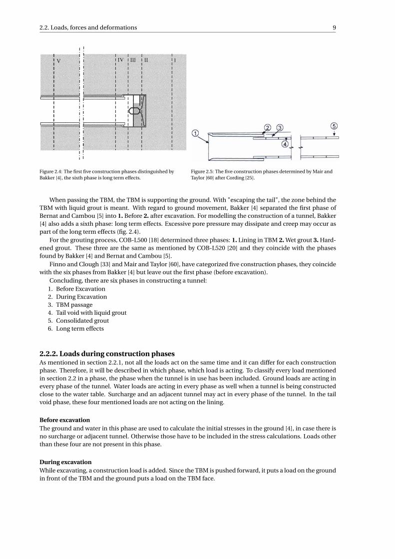
Figure 2.4: The first five construction phases distinguished byBakker [4], the sixth phase is long term effects.
Figure 2.5: The five construction phases determined by Mair andTaylor [60] after Cording [25].
When passing the TBM, the TBM is supporting the ground. With "escaping the tail", the zone behind theTBM with liquid grout is meant. With regard to ground movement, Bakker [4] separated the first phase ofBernat and Cambou [5] into 1. Before 2. after excavation. For modelling the construction of a tunnel, Bakker[4] also adds a sixth phase: long term effects. Excessive pore pressure may dissipate and creep may occur aspart of the long term effects (fig. 2.4).
For the grouting process, COB-L500 [18] determined three phases: 1. Lining in TBM 2. Wet grout 3. Hard-ened grout. These three are the same as mentioned by COB-L520 [20] and they coincide with the phasesfound by Bakker [4] and Bernat and Cambou [5].
Finno and Clough [33] and Mair and Taylor [60], have categorized five construction phases, they coincidewith the six phases from Bakker [4] but leave out the first phase (before excavation).
Concluding, there are six phases in constructing a tunnel:1. Before Excavation2. During Excavation3. TBM passage4. Tail void with liquid grout5. Consolidated grout6. Long term effects
2.2.2. Loads during construction phasesAs mentioned in section 2.2.1, not all the loads act on the same time and it can differ for each constructionphase. Therefore, it will be described in which phase, which load is acting. To classify every load mentionedin section 2.2 in a phase, the phase when the tunnel is in use has been included. Ground loads are acting inevery phase of the tunnel. Water loads are acting in every phase as well when a tunnel is being constructedclose to the water table. Surcharge and an adjacent tunnel may act in every phase of the tunnel. In the tailvoid phase, these four mentioned loads are not acting on the lining.
Before excavationThe ground and water in this phase are used to calculate the initial stresses in the ground [4], in case there isno surcharge or adjacent tunnel. Otherwise those have to be included in the stress calculations. Loads otherthan these four are not present in this phase.
During excavationWhile excavating, a construction load is added. Since the TBM is pushed forward, it puts a load on the groundin front of the TBM and the ground puts a load on the TBM face.

10 2. Literature Review
TBM PassageWhen the TBM passes, excavation has taken place. The tapered shape of the TBM leaves a void behind afterthe bore front has passed. This void is filled with grout adding a grout pressure load on the ground. The voidmay allow the soil to contract, adding the possibility of a subgrade reaction. The TBM itself is now present,which results in some additional loads. The weight of the TBM is one, but the heat that the TBM produces,poses an extra temperature load as well.
Tail void with liquid groutIn the tail void, the tunnel lining has left the TBM. This means the weight of the TBM is not present in thisphase. The backup train attached to the TBM is present and therefore its weight. Jacking by the TBM onthe tunnel lining is now added as a construction load. The tunnel weight itself is also present, posing anadditional load. The ground and water pressure are present but they are acting on the liquid grout. The sameaccounts for surcharge and subgrade reaction. The grout pressure takes all the pressure coming from outsidethe tunnel and exerts those onto the tunnel lining. Therefore ground, water, surcharge and subgrade reactionare present, but when considering the lining, only the grout pressure is acting.
Consolidated groutIn this phase, the grout has completely consolidated and therefore no grout pressure is active any more. Thegap can now be considered closed and from now on the ground and water pressure (and surcharge) will beacting on the hardened grout and thus the lining.
Long term effectsFor the long term effects, the ground and water pressure may alter. If the boring has caused excessive porewater pressures, these will now dissipate [33]. Creep effects may also occur in this stage [4]. The TBM has nowmoved forwards so much that no construction loads are present any more, also not from the follow carts. Thetemperature load has switched from being caused by the TBM towards being caused by seasonal temperaturechanges. Long term is a statement which may consume a large timespan. Therefore the line between the longterm and ’in use’ phase cannot be specified clearly.
In useFinally the tunnel can be taken into use and the traffic, special and loads from inside have to be taken intoaccount. Long term effects described at phase 6 may also still occur.
Phases
1 2 3 4 5 6 7
before during TBM tail consol. long in use
excav. excav. passage void grout term
tunnel weight x x x x x
ground pressure x x x x x x
water pressure x x x x x x
grout pressure x x
surcharge x x x x x x
subgrade reaction x x x x
loads from inside x
construction loads x x x x
temperature load x x x x x x x
traffic loads x
adjacent tunnels x x x x x x
Load
s
special loads x
Table 2.1: Overview of the loads present for each phase of the tunnel construction.

2.2. Loads, forces and deformations 11
2.2.3. Lining deformationsAll these loads cause the tunnel lining to deform or displace and multiple types are possible [18]:
1. global deformation of tunnel axis2. ovalisation3. displacement of rings4. buckling
With regards to the global deformation of the tunnel axis, the realised alignment deviates from the plannedone. Vertical or horizontal displacement of the tunnel lining causes this deviation. The vertical displacementcan be caused by settlements underneath the tunnel, but "negative" settlements also may occur. This iscaused by buoyancy as described in section 2.2. At the start and receiving shaft, the tunnel is fixed and nodisplacement can occur, only rotations. If vertical or horizontal displacement of the tunnel occurs, the tunnellining is bended, causing additional loads in the tunnel lining. This phenomenon will be discussed in section2.3.3. Moreover, if the alignment differs, it may not satisfy the requirements any more.
This settlement or buoyancy may also cause the rings to displace relative to each other. This will happenwhen the local shear resistance of the joints is exceeded, more about this will be discussed in section 2.3.4.
The most important deformation type is ovalisation. This is applicable to a tunnel ring. For ovalisation,the vertical loads at the crown and bottom of the tunnel are the largest while the horizontal loads at the sidesof the tunnel are smaller (fig. 2.6a). This deforms the tunnel into an oval with the sides of the tunnel movingoutward laterally and the crown and bottom move inward vertically (fig. 2.6b). This happens since the tunnellining needs to find the right ground reaction in order to reach an equilibrium between the loads [2]. Thisdeformation leads to bending of tunnel segments and rotations of joints about which will more be discussedin section 2.3.4. In the rare case of larger horizontal than vertical loads, vertical ovalisation can occur as well.Blom [7] discusses the ovalisation loads and how they migrate through the joints in his thesis.
(a) Ovalisation load [2] (b) Ovalisation deformation [18]
Figure 2.6: Ovalisation load (a) and the deformation caused by this load (b).
There is one more deformation type and it is called buckling. It happens when the tunnel lining is not ableto withstand the forces any more due to large deformations of the lining [7]. There are three ways for bucklingto happen [18]. 1. folding of beam: The global deformations may lead to bending which cause the tunnel thefold. If the lining is unable to withstand the generated force, this may cause the lining to snap trough. This isvery unlikely to happen due to the favourable ratio of lining thickness and tunnel diameter. 2. Snap through:In a tunnel ring, the segments cannot withstand the normal force and cause them to snap through. 3. Jointshearing: The shearing resistance cannot withstand the forces on the lining and one segment buckles throughshearing along a longitudinal joint. This is more common to occur for special loads like explosion or collisionloads.

12 2. Literature Review
(a) Snap through (b) Shear buckling
Figure 2.7: Two types of buckling deformation of tunnel lining [18].
2.2.4. Slip or bonded ground-lining interactionThese deformations depend on how the load is acting on the tunnel lining. The interaction between theground and lining plays an important role. For modelling this interaction, two extremes can be chosen for theboundary of the tunnel lining with the soil. These extremes provide two boundaries between which the actualstress state of the lining can variate [21]. The tunnel lining is fully bonding with the surrounding ground, soat the interface between the ground and the lining there is friction. There can also be no bonding at all whichmeans there is no friction at the interface between the lining and the ground. These two options are called"bond" or "slip" modelling respectively. For bond modelling, the ground is perfectly attached to the lining.This may cause shear stresses to develop between the ground and lining. With slip, these tangential stresseswill not be transferred between the soil and the lining [65]. Slip may be caused by grouting, ground water andtemperature differences. This will lead to a reduction of the effective stress below the tunnel [18]. Modellingslip or bond translates into a difference in bending moment for different calculation methods. For bond, allthe calculation methods have approximately the same bending moment results. While for slip, the differentcalculation methods differ in moment results [16].
2.3. Tunnel lining designFor designing a tunnel, different design approaches are available. The internal forces in the tunnel lining canbe calculated by using analytical or numerical methods. These methods are used for different calculationmodels which are divided into ring and beam action models.
2.3.1. Schulze-Duddeck methodOne of the first methods developed was the method by Schulze and Duddeck [71]. Many German bored tun-nels have been constructed based on this theory and even nowadays it is still used in preliminary designs.While trying to approach reality as close as possible, the complexity of the models and calculation was keptas low as possible. Therefore, assumptions have been made in this method:
• Soil only supports the tunnel in a radial direction. The soil and tunnel can move free from each otherin the tangential direction [18].
• The surrounding soil behaves linear elastic and deforms under plane strain conditions [18].• The soil loading on the lining is determined from the initial soil loads of untouched ground at the depth
of the tunnel axis [18]. This also assumes that the ground wants to return to the same state as it wasbefore the construction of the tunnel [32]. From the converted loads, the forces in the lining are deter-mined from ground-lining interaction graphs proposed by Schulze and Duddeck [71].
• Clay and peat have not been included in the graphs and therefore it is questionable whether this methodcan be used in Dutch conditions [58].
• The hydrostatic pressure is not increased along the tunnel depth. This is assumed in other to meet aload equilibrium [18].
• The depth is of great importance with this method. Three different areas can be distinguished basedon the height of the overburden and the diameter of the tunnel.
– height < two times the diameter– two times the diameter < height < three times the diameter– height > three times diameter

2.3. Tunnel lining design 13
For the overburden height smaller than two times the diameter, support is only applied on the part ofthe lining where it deforms outward. This mean than 90°along the crown of the tunnel is unsupportedby the soil. When the overburden height is larger than three times the diameter, the entire ring willbe supported by the soil. If the overburden height is between two and three times the diameter, it isdepending on the cohesion of the soil whether the top of the lining is supported or not [9, 18, 56].
• One homogeneous soil layer is located around the tunnel lining. So this method is not applicable whenthe tunnel crosses multiple soil layers [1, 18].
• The tunnel is made of an homogeneous ring. Joints are not applied in this method [58].• The force distribution by Schulze and Duddeck [71] does not apply for liquid grout. It can be used for
consolidated grout, but this approach does not take into account the liquid grout circumstances [8].
While many assumptions have been made, this method is still widely used. As can be deducted from thedifferent assumptions, different phenomena are present in the structural behaviour of a segmental tunnellining. The complexities of these phenomena cannot be taken into account with this method. A few of thesephenomena and its complexities are described in sections 2.3.2, 2.3.3 and 2.3.4. These complexities can bemodelled in finite element programs.
2.3.2. Ring actionIn the ring action model, it is assumed that along the axis the loads are the same or deviations are too smallto be included. Therefore, one ring of the tunnel lining is schematized together with the surrounding soil andonly circumferential directed lining stresses are included.
Within a ring model, the ground is either schematized as discrete springs, two-dimensional or three-dimensional elements.
Discrete SpringsWhen using the discrete springs, the tunnel is modelled as a elastic supported ring which is stiff for bothbending and strain. The discrete springs are the support of the tunnel. The tangential and radial stiffnessfor the springs are not connected and can be developed separately. The radial and tangential loads from theground are directly attached to the lining. Furthermore, it is a one-dimensional model and therefore spatialeffects cannot be taken into account. These discrete springs models can be calculated by using an analyticalmethod [56].
2-dimensional continuumThe schematization of the problem with two-dimensional elements is a finite element method in which acontinuum model is discretized. These finite element methods are more complex than the discrete springmodel. For a preliminary design, analytical methods are often used. For final design or special effects, finiteelement methods are used. Some effects, for example the influence of soil layering, cannot be modelled withthe discrete spring model described in section 2.3.2. However, the complex behaviour of the ground can bedescribed by using material models for the soils in the finite element programs [56], including the influenceof soil layering.
3-dimensional continuumTunnel excavation is a three dimensional problem [35]. Especially in the Netherlands the third dimension intunnel lining design plays an important role. Because of the soft soils in the Netherlands, of which the prop-erties can vary significantly, differential settlements may occur. If this happens, the tunnel lining is loadeddifferently along the axis of the tunnel. This non-uniform loading over the tunnel axis causes a change ininternal forces in the tunnel lining. When modelling the problem with three-dimensional elements, both thering action as well as the beam action are included, more about beam action will be discussed in section 2.3.3.
2.3.3. Beam actionAs described in section 2.3.2, the load conditions in axial direction on the tunnel lining may vary. This canhappen for various reasons [9]:
1. Difference in supportWhile the tunnel load may be distributed equally, differential settlements can be caused by differ-ences in stiffness for the supporting soil underneath the tunnel. The differential displacements cause achange in internal forces in the tunnel lining;

14 2. Literature Review
(a) (b)
Figure 2.8: A spring model (a) and a continuum model (b) for radial action [58].
2. Unequal soil loadingThe soil above the tunnel can be unequally loaded. Either by another tunnel that crosses the new tunnelor at the surface by buildings and roads. This unequally loaded soil can result in differential settlementsof the soil and therefore unequal loading on the tunnel lining;
3. ConsolidationThis may cause differential settlements over time and therefore create a change in internal forces;
4. Fixated start and endAt the start and end shaft, the tunnel is fixated. No vertical displacement will occur while rotating ispossible. This can also lead to a change in internal forces;
5. Construction loadsDuring construction, there is the load of the tunnel boring machine and everything that follows. Fur-thermore, a tunnel boring machine can also change course. Both bring an extra load on the ground andtunnel lining and may cause differential loading as well;
6. BuoyancyThe tail void is injected with liquid grout. While the grout is liquid, the tunnel may suffer uplift until thegrout is solidified. The uplift can cause a change in internal forces [18].
The analysis of these load conditions is called the beam action [58]. These loads can cause the tunnel tobend (figure 2.9a). Apart from the three-dimensional model described in section 2.3.2 in which both beamaction and radial action are included, there is also a one-dimensional beam action model (figure 2.9b). In theone-dimensional model, the mechanics of the tunnel and the supporting ground can be set. Like with ringaction, the ground is schematized by discrete springs [56]. In the three-dimensional model, the effect of thevariation in load conditions in the axial direction can only be modelled by using multiple rings.
(a) (b)
Figure 2.9: Bending of the tunnel lining (a) and a simplified one-dimensional model of beam action (b) [58]

2.3. Tunnel lining design 15
Types of beamsBending of the tunnel causes an internal bending moment. Besides this moment, another internal force mayoccur in the tunnel lining for beam action, shear force. Therefore a tunnel can be considered as two types ofbeams or a combination of those types, a shear and a bending beam (figure 2.10). A nice explanation of thestructural theory behind these beams is given by Bouma [10].
(a) (b)
Figure 2.10: A bending beam (a) and a shear beam (b) [10]
2.3.4. JointsBoth for radial and beam action, a critical issue has to be included in the lining design. In shield tunnelling,the lining is constructed in segments, as previously mentioned in chapter 1. Erecting the lining from seg-ments has the consequence that a ring is a structure with multiple hinges. Furthermore, placing rings next toeach other creates an extra hinge in the tunnel lining as well. These hinges are called joints and two types canbe identified: longitudinal and circumferential joints. The longitudinal, radial or segment, joint is located be-tween two segments in one ring. The circumferential, lateral or ring, joint is located between two consecutiverings (figure 2.11).
To ensure longitudinal joints are not continuous, usually a staggered configuration of the segments isapplied, the so called masonry layout. Multiple elements can be present in a joint [56]:
1. Bolts (non/temporary/permanent)2. Connection system3. Packing material4. Water seal
Bolts are applied to connect the segments and increase the bending stiffness of the tunnel, on which willbe elaborated in section 2.3.4. Bogaards [9] shows different types of bolting.
Connection systemsThere are also different kinds of connection systems between segments. The most used systems are:
1. Flat2. Tongue-groove3. Dowel-socket4. Convex5. Cam-pocket system
For a flat connection system, it can either be flat over the entire thickness of the segment (figure 2.12a)or it can have a reduced contact area (figure 2.12b). With a flat joint, the coupling between segments is onlythrough friction and it supports itself without purposely interacting with other segments [59]. The flat surfacedoes allow rotation and therefore can transfer bending moments. The tongue-groove is usually applied in thecircumferential joints and consists of a groove in one of the rings while the connecting ring has a tongue

16 2. Literature Review
Figure 2.11: Definition of circumferential and longitudinal joint [24].
shape that fits with the groove (figure 2.12c). The dowel-socket system is a variant on the tongue-groove sys-tem but the groove is deeper and the tongue is higher. This allows it to be reinforced [24]. Another variantto the tongue-groove system is the convex-concave system (figure 2.12d). Another connection system is thecam-pocket system which is a point coupling system (figure 2.12e). The loads in this system are more lo-cally restricted compared to distributed over the entire ring joint in the tongue-groove system. The last foursystems help to centre the segments during placement and also limit the displacement differences betweensegments [7].
These systems cause two rings to come in contact. An un-smooth surface may lead to local peak stressesfor concrete-to-concrete contact. This can be countered by using packing materials. These packing mate-rial types will introduce the internal forces into the next ring and two types are commonly used: plywoodand kaubit. A shear force may develop in the plywood when different deformations occur in adjacent rings.This friction with the concrete will establish a cooperation between the two rings. Long term effects of theplywood, however, are unknown in terms of durability [58]. Koek [53] mentions that if the plywood totallydeteriorates, the axial normal force may disappear completely. Kaubit is a bituminous material and has avery low stiffness. The transfer of internal forces by kaubit is unknown [24]. In compression, the kaubit willdeform and increase the contact area. When compression is increased, at one point the kaubit is thinned outand concrete-to-concrete may occur again [58].
A tunnel needs to be watertight. The segments itself ensure watertightness, the joints do not. Therefore, awater seal is included that has to ensure watertightness even during deformations of the lining. The seals aremade of neoprene or hydrophilic rubber. The neoprene profile will ensure watertightness when it is loadedby internal forces. The hydrophilic rubber will increase in volume when in comes in contact with water andthus ensure watertightness [9].
Bending stiffnessThese joints decrease the bending stiffness of the tunnel. In the axial direction, the circumferential joints andthe tunnel rings work in series. For a ring, the stiffness is also reduced because of the longitudinal joints. Thebending stiffness of the joints is depending on the connection system as described in section 2.3.4. It dependson the geometry, its mechanical properties and the properties of the packing material [56].
The decrease in bending stiffness, caused by the joints, has a large influence on the structural behaviourof the tunnel lining [30, 52, 54, 58, 78]. In order to include this decrease in bending stiffness, a reduction canbe given to the bending rigidity. This can vary between 0.5 and 1.0 [17, 54].
Another way to include the joint in the tunnel lining is by approaching the joint as a hinge with or without

2.3. Tunnel lining design 17
Segment
Segment
(a) Flat joint
Segment
Segment
(b) Reduced flat [7]
Segment
Segment
Tongue
/Dowel
Groove
/Socket
(c) Tongue-groove (dowel-socket) [7]Segment
Segment
(d) Convex-concave [58] (e) Cam-pocket [61]
Figure 2.12: Five connection systems for construction of segmental tunnel lining.
a rotational stiffness. This is done for longitudinal joints in which the segments rotate relative to each other.In the case of an uniform radial pressure on the tunnel lining, a normal force will be acting in the joint.The joint height is the contact area between the segments. When this is small compared to the thicknessof the segment, the forces will be transferred in a concentrated way. The hinge has a resistance to rotating,which causes a bending moment to occur. The rotating stiffness is derived from the theory of Janssen [45]and depends on contact area, tangential normal force and the rotation [7]. A small contact area may lead toadditional curvatures and therefore rotations. This is applicable when the joints are still closed, also calledthe linear branch of the joint behaviour. The joint can also open, this is called the non-linear branch. Theopening of a joint leads to a decrease in rotational stiffness of the joint. A joint can only open up when thepressure on the outer side of the contact area becomes zero. Bogaards [9] elaborates on the gaping of joints.
Janssen’s theory is a theoretical model which describes the relation between the moment and rotation ofa joint in segmental tunnel lining. It is based on the theory of concrete hinges. Janssen schematized the lon-gitudinal joint as an equivalent concrete beam with the same properties. This beam is loaded by a bendingmoment and simulates the rotation and the additional curvatures in the adjoining segments. These curva-tures are caused by the introduction of the concentrated force into the segments. Equation 2.1 & 2.2 give therelation between moment and rotation for the linear and non-linear branch respectively [58].
φ= Mh
E I= 12
M
Eh2b(2.1)
φ= 8Fn
9bhE( 2MFn h −1)
(2.2)
Janssen’s method was the first, widely used method for including joints in tunnel lining. Since, other an-alytical solutions have been presented. Gladwell [37] also presented a moment-rotation relation. Blom [7]presented an adaptation to Janssen’s method. These three methods are compared briefly by Luttikholt [58].
The circumferential joints have to be approached when the tunnel is discussed along its axis. In this joint,rotation and translation may occur. When no packing material is applied, a shear force may develop causedby the concrete-on-concrete contact that will counteract the mutual radial and tangential deformations. Thisalso gives a resistance against rotations. The shear force is dependent on the normal force in the joint, thecontact area and its smoothness. Moreover, an unsmooth surface may results in high speak stresses. Withpacking material two shear deformations may occur. The mutual deformations may be counteracted by theshear force developed because of the friction between the packing material and the concrete. It can also becounteracted by the shear deformation occurring in the packing material [58].

18 2. Literature Review
These joints are approached by using coupling springs. The dowel and socket connection system is themost approached connection system for circumferential joints. Coupling springs describe the behaviour ofthis system and also describe the lateral friction between the concrete and the packing material, as describedabove. These linear springs can only handle normal force and are radially orientated [7]. The approach by-Blom [7] starts with equation 2.1 and continues on the deformations induced by rotation in the longitudinaljoints. He further elaborates on these deformations by adding the bending stiffness and the soil. Eventu-ally the circumferential joints are included and coupled rings are acquired. The influence of coupled rings issignificant [52]. Finally, an elastic soil continuum is added to the coupled system and the approach is com-pleted.
While the joints are discussed by using analytical models, in FEM the joints are sometimes also modelledas springs. Either as rotational springs for the longitudinal joints or lateral springs for the circumferentialjoints. The non-linear behaviour as discussed can also be applied to those springs in FEM modelling [52].More about modelling of the joints in finite element programs will be discussed in section 2.4.
2.4. Finite Element Method Programs
In this section, a short overview is given of the different programs that have been found suitable to modelthe construction of a tunnel. This overview has been created by examining the website and manuals of theprograms as well as articles in which the program is mentioned. The advantages and disadvantages will bediscussed and a verdict will be given for each program on its tunnel modelling capabilities. The comparisoncriteria searched for in the documents are:
• Soil Models: Availability of soil models on which will be elaborated in section 2.6;• Concrete Models: Availability of concrete models;• Joints: Modelling of joints;• Slip and Bond: Modelling of slip and bond;• Interfaces: Closely related to the above two points; modelling and use of interfaces;• Elements: Availability of element types;• Phases: Modelling of phased construction;• Results: What can be calculated and how it can be plotted;• Specific tunnel application: If is advertised or mentioned that tunnelling is one of the applications;• Ease to work with: Interface or programming input and available documentation;• Design approaches: Extra features for design, for example designing with a Eurocode;
2.4.1. Plaxis
Plaxis is well known for its modelling of the subsurface. This can also be seen in the amount of constitutivesoil models that are present in the program, more than any other program discussed in this section. Withregards to the lining, Plaxis does not have specific concrete models but it does have linear models that canbe applied with concrete properties. In the 2D version of the program, segmental joints can be modelled ashinges. For the 3D version, no solution for modelling the joints has been found in the documentation exceptfor reducing the stiffness to account for the joints. The contact between lining and soil can be modelled withan interface that consists of joint elements with its own friction angle and adhesion. With regards to theelements used in the model, for soil many high-order volume elements are available and for the lining, plateand beam elements. With these structural elements, the structural forces can be measured and displayed.The same accounts for the displacements. Different types of plots are available for displaying the results, forexample vector and contour plots. Phases can be implemented in which elements can be activated as well asde-activated. This way, a staged construction can be modelled. Plaxis has a tunnel designer module insidethe program, which makes modelling a tunnel more simple. Besides this module, Plaxis works with a userinterface for input and a lot of documentation is available. Different manuals for reference of the programfeatures are available as well as a manual for the scientific base for all the different calculations in the program.The constitutive models are also explained extensively and there is a tutorial manual. For many geotechnicalissues, a tutorial is available on how to model this in Plaxis, this includes tutorials for tunnelling. Furthermore,an extra feature in Plaxis is able to define a coherent set of parameters and partial factor according to ultimatelimit state design methods, apart from the serviceability limit state calculations [12].

2.4. Finite Element Method Programs 19
2.4.2. DIANAMany constitutive models are available in DIANA. Furthermore, it also has some concrete models that canbe used for lining, besides the linear elastic models. These concrete models can model non-linear behaviourand incorporate cracking as well. For the modelling of the joints, special elements are available called contactand interface elements. A Janssen characteristic (as shortly described in section 2.3.4) can be applied tothese elements. Also for the interaction between the lining and the soil, interface elements can be used withnon-linear behaviour. A few special elements have already been mentioned, but there many other typesavailable in DIANA, including shell and solid elements. Phased construction can be applied. For displayingthe structural forces results, different plot types are available. Tunnelling is a major focus of DIANA, as can bededucted from DIANA FEA BV [27]. This also shows from the amount of tutorials available. While there aremany, they are not all for the same pre-processor. DIANA has multiple pre-processors of which one uses aprogramming input and another uses a user interface. For the latter, DIANA is currently creating the tutorialsso there are not a lot available yet. Besides the tutorial, a large amount of documentation can be found intheir online manual, this includes user guides and reference material. Designing according to the Eurocodeis an extra mentionable feature in DIANA [27].
2.4.3. CESAR-LCPCCESAR has many constitutive soil models: several linear and non-linear elasticity models and many plastic-ity soil models. Besides for soil, there are also some plasticity models for other materials available, includingearly age concrete [44]. Whether lining joints can be modelled remains unclear. There are interface and springelements available, but it is not highlighted they can be used for lining joints. The interface elements are ableto model slip and bond. Three contact models are available for these interface elements: Coulomb’s friction,bonding, perfect slippage. Besides the interface and spring elements, there are volume elements availablefor the soil and trusses, beams and shells as structural elements. Phased construction is available by removalor addition of clusters, the confinement forces are also automatically generated. From the beam and shellelements the structural forces can be shown in a 3D view. Furthermore, there are cross sectional planes andiso-surfaces available [43]. While tunnelling is one of the main applications of CESAR, other geotechnical andstructural issues can also be modelled. This is done through an input interface. With regards to documen-tation, information about the constitutive models [44] and a brochure about the programs features [43] areaavailable. There is also a user guide available but that does not contain much more information than in thebefore mentioned documents. Tutorials, however, are scarce. There are some tutorial videos but these do notcontain complicated problems. Factor of safety calculations can also be donein CESAR [43].
2.4.4. GTS NXGTS NX is a program developed by Midas and can be bought as a pre- and post-processor for DIANA or astandalone program, which will be discussed here. It has both elastic and plastic material models, but mostlyfor soil and no specific concrete models. There are also interface models available: Janssen and Coulomb fric-tion. This Janssen model can be used on the interface elements that represent the joints, while the Coulombfriction can be used for the soil-structure interface elements. Other element types are also available, for ex-ample truss, beam and shell elements [63]. Phases can be implemented as well, it is emphasized this can beused for shield TBM analysis in which the structural forces are obtained for every phase [62]. These forces canbe displayed through cross-section and contour plots amongst other display options [64]. It is obvious thattunnelling is an application for GTS NX. This can also be seen from the amount of tunnelling tutorials. Bothfor 2D and 3D there are tutorials, there is even a tutorial for shield TBM analysis. Besides the tutorials, thereis also documentation for reference and verification and a user guide. As input, GTS NX uses a user interface.It is not clear whether extra features like the factor of safety calculations or Eurocode designing are present inGTS NX.
2.4.5. OtherThese five programs are not the only finite elements programs that have been used for tunnelling. These arethe five however that have been deemed to be the most suitable based on the criteria given at the beginningof this section. There are some programs however that should be mentioned and explained why they werenot further reviewed.

20 2. Literature Review
AbaqusAbaqus is a multipurpose finite element program. While tunnels can be modelled in this program as doneby [51, 57, 68], Abaqus itself does not promote or mention it. Therefore no tutorials for tunnel modelling inAbaqus can be found. There is one document on their website about a tunnel plugin for Abaqus. In this doc-ument Fioranelli Jr et al. [34], discusses that the Abaqus interface is not user friendly for tunnelling analysisand that therefore the plugin has been developed. Abaqus only has two plastic constitutive soil models aswell. Further elaboration on Abaqus has not been done based on these criteria.
AnsysAnsys is excluded from further elaboration for almost the same reasons as Abaqus. Multiple authors [7, 8,16] have modelled tunnels in Ansys. Nowadays, little documentation by Ansys can be found with regardsto tunnelling. Many tutorials are available but none of them are about geotechnical issues. Lengkeek [56]already stated that Ansys is more focused on structural than on geotechnical. issues. Another program called"CivilFEM" can be used to make working on geotechnical issues in Ansys easier.
Tochnog ProfessionalThis program has many soil constitutive models but lacks the structural approach. Joints cannot be modelledand no information can be found about whether the structural forces in the lining can be modelled. Theavailable tutorials are not for tunnelling problems either. Based on these criteria, Tochnog Professional is notfurther reviewed.
RS3
This program has been developed by Rocscience. The ground can be modelled by many different constitutivemodels, only the lining cannot be modelled correctly. Joints cannot be modelled and it is unclear whether thestructural forces in the lining can be measured in this program. Therefore it is not further reviewed.
Flac3DFlac3D is also a program which can model geotechnical issues including tunnelling. However, it is a programwhich uses the finite difference method instead of finite element. This is the reason is has not been includedin further reviewed since only FEM will be investigated.
2.4.6. ConclusionTable 2.2 provides a summary on how the different programs score on the criteria. It is clearly visible thatbased on these criteria, DIANA is considered the best program for modelling the tunnelling process, followedby GTS NX and Plaxis. This has only been based on the available documentation of the different programs.A real conclusion on these programs can be given when the program is used for modelling the tunnellingprocess and results have been compared. It has been decided to assess the possibilities of modelling the con-struction phases of bored tunnels in DIANA and Plaxis. DIANA comes out as the most suitable program basedon the available documentation and Plaxis, while not being second, is widely used in the geotechnical, andthus tunnelling community, in the Netherlands. Therefore the Plaxis is favoured for assessing the possibilitiesover GTS NX.
2.5. Parametric studiesIn tunnelling, many different parameters are present and require input when modelling the soil and lining.However, not all parameters have the same influence on the problem. This section elaborates on parametricstudies that have been performed on the influence on the tunnel lining forces.
2.5.1. Soil parametersFirst, the influence of soil parameters on the lining forces will be discussed.
Young’s modulusFor a stiff ground, thus a high Young’s modulus, a circular excavation in the ground will lead to less conver-gence of the soil into the excavation. When the soil is less stiff, more convergence will occur. This will lead tomore loading on the lining. An increase in Young’s modulus will result in a decrease in the internal forces ofthe lining [2, 30, 55, 66, 70]. This includes the shear force [46].

2.5. Parametric studies 21
Programs
Plaxis DIANA CESAR-LCPC GTS NX
Soil Models ++ + + +
Concrete Models +/- ++ + +/-
Joints +/- ++ - ++
Slip and bond + ++ ++ +
Interfaces + + + ++
Elements + ++ ++ ++
Phases ++ ++ + ++
Results ++ ++ ++ ++
Specific tunnel application ++ ++ ++ ++
Ease to work with ++ + +/- ++
Cri
teri
a
Design Approaches + ++ + -
Table 2.2: Summary of the different FEM programs and their scores on the criteria.
Lateral earth pressure coefficientThe bending moment is the lowest when the lateral earth pressure coefficient is at unity. Moving away fromunity, either increase or decrease, leads to an increase in bending moment [30, 66, 70]. When the lateralearth pressure coefficient is at unity, the vertical and horizontal load are equal. Moving away from unity, thedifference between vertical and horizontal load increases and therefore the bending moment in the liningwill increase as well. An increasing lateral earth pressure coefficient will lead to an increasing normal force[30, 70].
Poisson’s ratioWhile the Poisson’s ratio does not have an influence on the normal force in the tunnel lining, it does affect thebending moment. An increase in Poisson’s ratio leads to a slight decrease in bending moment [70] and shearforce [46].
CohesionCohesion does not have an influence on the bending moment. An increase in cohesion does lead to a slightdecrease in normal force [66, 70]. More cohesion means less convergence in a circular excavation, thereforethe normal forces in the lining will decrease.
Friction angleWith more research needed, Möller and Vermeer [66] state that the friction angle has little influence on theinternal lining forces. Kasper and Meschke [50], Palassi and Mohebbi [70] state that with an increase in fric-tion angle the normal force will decrease. A higher friction angle means more load is taken by the soil itself,this causes the radial loading to decrease and therefore the normal forces in the lining. For the bending mo-ment, they are in disagreement. Kasper and Meschke [50] state that an increase in friction angle will leadto a slight increase in bending moment while Palassi and Mohebbi [70] states that the bending moment willslightly decrease.
Overconsolidation ratioAn increase in overconsolidation ratio leads to a slight decrease in normal force in the lining. With a lowoverconsolidation ratio, plastic deformations of the soil around the tunnel are large. The reduction of thisplastic deformations when increasing the overconsolidation ratio, causes the lining pressure to decrease aswell and therefore the normal force. The bending moment is hardly influenced by the overconsolidation ratio[50].
PermeabilityThe permeability has little influence on the bending moment and normal force in the tunnel lining. Whetherthese forces slightly increase or decrease with increasing permeability depends on the location at the tunnel

22 2. Literature Review
ring. The pore pressures around the tunnel are influenced by the grouting pressure, the support face pressureand the buoyancy [50].
2.5.2. Tunnel parametersApart from the soil parameters, the project (or tunnel) parameters also have an influence on the tunnel lining.
Cover depthKasper and Meschke [50], Katebi et al. [51], Palassi and Mohebbi [70] state what many authors state: an in-crease in depth for the tunnel leads to an increase in internal forces. The increase in overburden height andhydrostatic pressure with the depth cause an increase in the lining pressure. The difference between thepressure at the crown, bottom and sides of the tunnel also increases, which increases the bending moment.The increase in depth also leads to an anticipation of pressure in the excavation chamber. More pressure isneeded in that chamber to resist the soil and therefore the jacking forces and the axial loading will increase[50].
Tunnel radiusThe tunnel radius is usually already set in the project, but it does have an influence on the internal forces ofthe lining. When the tunnel radius increases, the bending stiffness of the lining decreases. This leads to adecrease in bending moments as well. Furthermore, because the radius increases, the pressure on the liningincreases. This leads to an increase in normal force in the lining [70].
Face support pressureThis pressure has already been mentioned discussing two other parameters and their influence on the inter-nal forces of the lining. An increase in face support pressure causes the stress release in front of the TBM todecrease. Therefore there will be a slight increase in the lining pressure and thus the normal force in the lin-ing. The difference in pressure surrounding the tunnel decreases so the bending moment decreases as well.For the axial loading, the same accounts as discussed with the influence of the tunnel depth [49].
Grouting pressureGrouting pressure causes the same type of soil response as the face support pressure. When it is increased,the stress release of the soil is decreased. The lining pressure and the normal force increase, the bendingmoments decrease [49].
Hydration characteristics groutGrout hardens towards a final strength and stiffness. The final values of this strength and stiffness are impor-tant, but not as important as the time it takes to get to that values. When the grout hardens quicker, therewill be less time for the soil to release the stress. The lining pressure will increase causing the normal force toincrease as well. When the hardening time is short, there will still be some upward movement from the soilbelow the tunnel caused by the TBM passage. Combined with the reduction in stress release, this will lead toan increase in pressure at the bottom of the tunnel. This causes the bending moments to increase [50]. Moreabout the grouting and its characteristics will be discussed in section 2.8.1.
TBM weightThe TBM is located in front of the lining, so it does not exceed a pressure on the lining directly apart fromjacking forces and this axial pressure. However,the weight does have an influence on the radial pressure onthe lining. Underneath the TBM, the ground settles under the weight. This results in a heave of the soil assoon as the TBM has passed. Behind the TBM, the lining is already in place. So the heave results in a radialpressure on the lining. An increase in weight will results in more settlement and therefore more heave. Theincreased lining pressure due to the heave will cause the normal force and bending moments to increaseslightly [49].
TBM lengthApart from the weight, the TBM also causes deformation through frictional interaction between the shieldskin and the soil. Softening occurs at the sides of the tunnel and increases with increasing TBM length, whichleads to a decrease in lining pressure at that location. With little changes at the crown or bottom, an increasein bending moment and decrease in normal force occur. For a longer TBM, the friction increases as well. Thatcauses the jacking forces, and thus the axial loading, to increase. The analyses in which this phenomena isinvestigated used overconsolidated soils in the model [49].

2.6. Soil models 23
TBM taperIf the taper is increased, the shape of the TBM becomes more conical. This leads to an increase in stressrelease of the surrounding soil. The lining pressure decreases causing the normal force to decrease and thebending moment to decrease slightly. The friction resistance is also decreased by an increasing taper andtherefore the axial loading is decreased [49].
Trailer weightThe trailer following the TBM has a weight and therefore has a pressure on the lining. This load is not dis-tributed evenly since the trailer is on wheels. In between two trailer loads, the pressure that the trailer exceedson the lining has a negligible influence on the lining forces. Kasper and Meschke [49] did not elaborate onthe influence of one trailer load directly on the lining. The trailer weight does counteract the buoyancy, anincrease in trailer weight would decrease the buoyancy.
2.5.3. Lining parametersThe lining is the last part in which different parameters can have an influence on the internal lining forces.
StiffnessJust as with the soil, the lining can have a stiffness. An increase in this stiffness leads to an increase in bendingmoment. The normal forces are not influenced by the lining stiffness [70]. Do et al. [30] also state that atunnel which deforms less has higher structural forces.
ThicknessThe thickness of the lining is related to the bending stiffness. When the thickness increases, the bendingstiffness increases.
Number of jointsA joint can decrease the lining stiffness depending on the joint’s stiffness, which will be discussed below.Therefore, the number of joints influence the lining as well. According to Do et al. [30] and Nikkhah et al. [69],this is only the case for the bending moment, which decreases with an increasing number of joints. This onlyaccounts for more than four joints.
Orientation of segment jointsThe orientation of the joints only influences the bending moment of the lining [30, 55]. The bending momenthowever also influences the influence of this joint. The joint’s influence is the largest when it is located at thelargest bending moment location [30].
Rotational stiffness of jointAs stated previously, a stiffer lining will result in higher internal forces. This is again applicable for the rotationstiffness of a joint. If this increases, the internal lining forces also increase [30, 55, 69].
Radial and axial stiffness of segment jointApart from the rotational stiffness, there are also the radial and axial stiffness of a joint. Both, however, havea negligible influence on the lining forces according to Do et al. [30].
2.6. Soil modelsThe soil can be modelled with different models, as previously mentioned in section 2.4. In this section, acouple of soil models will be described briefly. These soil models have been encountered in studies aboutmodelling the tunnelling process. The main reason for the different models is that not all soil types can berepresented by one model. The difference in behaviour is related to differences between soils but also theapplication is important with regards to choosing a soil model. Long term behaviour may be very differentthan short term behaviour for example.

24 2. Literature Review
2.6.1. Mohr-CoulombThe Mohr-Coulomb model is a simple model and is used to get a first approximation of the soil behaviour.This soil model is used in many studies [3, 5, 13, 14, 36, 46, 51, 79]. It is a linear elastic perfectly plastic modelthus no hardening or softening will occur [72]. Hooke’s law of isotropic elasticity is the basis for the elasticpart of the Mohr-Coulomb model. The perfectly plastic part is based on failure criterion by Mohr-Coulomb.With plastic behaviour, irreversible strains develop while with elastic behaviour, the strains will be reversedwhen unloading. The boundary between this elastic and plastic behaviour is given by the yield functionwhich is a function of the stress and strain. Since it is a perfectly plastic model, this yield function is fixedand only defined by its model parameters. This means that straining will not affect the yield function. Elasticbehaviour will occur with stress states that are located within the yield function and plastic behaviour willoccur for the stress states outside this yield function [12].
The Mohr-Coulomb requires five input parameters. An explanation about these input parameters is givenby Brinkgreve et al. [12]. The five input parameters are:
E Young’s modulusν Poisson’s ratioc Cohesionφ Friction angleψ Dilatancy angleσt Tension cut-off and tensile strength
2.6.2. Hardening SoilA more advanced soil model compared to Mohr-Coulomb is the Hardening Soil model and is also used inmany studies [40, 41, 67, 73]. First, in this model the stress-strain relation for primary loading is a hyperbola.Second, the yield surface is not fixed and plastic strain can cause it to expand which is called "hardening plas-ticity". Two types of hardening are included in the model. Shear hardening for the irreversible strains causedby primary deviatoric loading and compression hardening for the irreversible strains caused by primary com-pression in isotropic and oedometer loading. The shear hardening causes a decrease in deviatoric loadingand the compression hardening causes plastic compaction in primary compression and a difference betweenprimary loading and unloading and reloading. An elaborate explanation on this is given by Brinkgreve et al.[12]. With these differences, different input parameters are also needed. The last four parameters discussedfor Mohr-Coulomb in section 2.6.1 are also in the Hardening Soil model since the Mohr-Coulomb failurecriterion is still applied. The other parameters that are needed are [12]:
E r e f50 Secant stiffness in standard drained triaxial test
E r e foed Tangent stiffness for primary oedometer loading
E r e fur Unloading/reloading stiffness
m Power for stress-level dependency of stiffness
It can be seen from the list that one stiffness in the Mohr-Coulomb model (Young’s modulus), has beenreplaced by three different stiffnesses. These three cover the effects of the shear and compression hardening.
E r e f50 is used for the plastic strains caused by primary deviatoric loading (shear hardening). E r e f
oed is used forthe plastic strains caused by primary compression (compression hardening). Besides the plastic strains, com-pression hardening also included the difference between loading and unloading/reloading stiffness. This is
cover by the parameter E r e fur . The three stiffnesses are also related to a reference pressure because the Hard-
ening Soil model also accounts for the stress-dependency of these stiffness-moduli. This is covered by thepower "m". For some soft soils, other parameters may be used to calculate the stiffness parameters [12]. Con-version guidelines for Mohr-Coulomb parameters to Hardening Soil parameters are given by CUR [26]. The
Eoed parameters have to be converted to the reference oedometer parameter E r e foed by using the effective ver-
tical stress at the middle of the soil layer and converting that to a reference stress of 100 kPa. The conversion
includes the factor "m" of which indication values are given by CUR [26] as well. From the E r e foed , other con-
version rules are available for both clay and sand to acquire E r e f50 and E r e f
ur . The "m" chosen in the conversionalso has to be used in the Hardening Soil model for the corresponding soil layers.
The differences mentioned above are also mentioned by multiple authors [18, 72]. In other tunnellingprojects it is also mentioned that Hardening Soil might give better results on the structural forces in the

2.6. Soil models 25
lining than Mohr-Coulomb, just because of the stress-dependency and the different stiffness for unload-ing/reloading compared to primary loading [15, 23].
2.6.3. Hardening Soil small strainThe unloading/reloading behaviour in the Hardening Soil model is assumed to be elastic. However, this isonly the case for a very small strain range. The soil stiffness actually declines non-linearly with increasingstrain amplitude. Figure 2.13 shows the stiffness of the soil against the strain and shows a S-curve that reduceswith increasing strain. For the very small strains, the stiffness changes significantly. This can be taken intoaccount by the Hardening Soil small strain model.
Figure 2.13: Stiffness-strain behaviour of soil. Strain ranges for different structures have been indicated as well [12].
Since it is an extension on the Hardening Soil model, all its features will remain and so are its parameters.Two extra parameters are needed for the small strain stiffness.
G0 Very small-strain shear modulusγ0.7 Shear strain level when secant shear modulus is reduced to 70%.
2.6.4. (Modified) Cam-Clay(Modified) Cam-Clay is used by Finno and Clough [33] and Kasper and Meschke [48] for modelling soft cohe-sive soils, like clay, in there tunnelling model. It predicts the softening when dilatant plastic strains occur andhardening when contractant plastic strains occur. These two types of strains occur depending on the stressstate of the soil. The boundary between these two stress state areas is called the critical state line. There-fore, this line gives a relation between the mean principal stress and the deviatoric stress in state of failure.As with Hardening Soil, unloading/reloading does not follow the same relation as primary loading. This iscaused by the compression that may occur in soft, cohesive soils during primary loading and during unload-ing/reloading. A more elaborate explanation is given by Brinkgreve et al. [12], Kasper and Meschke [48]. Theinput parameters needed for the Modified Cam-Clay model are [12]:
νur Poisson’s ratioκ Cam-Clay swelling indexλ Cam-Clay compression indexM Tangent of critical state lineei ni t Inital void ratio
κ determines the compressibility of the soil during unloading/reloading while λ determines the com-pressibility of the soil during primary loading.
It is, however, recommended to not use this soil model for practical applications. Extremely large shearstresses may be allowed for particular stress paths, as well as softening may occur for particular stress paths.

26 2. Literature Review
This leads to practical problems like mesh dependency and convergence problems for iterative processes inthe finite element programs [12].
HypoplasticThe hypoplastic model has been created for describing state changes of granular materials and is an extensionto the critical state concept to which the Modified Cam-Clay models also belongs. These granular materialsare characterized by the current stress and void ratio. Instead of a Mohr-Coulomb or Drucker-Prager failurecriterion, the hypoplastic model has a failure criterion created by Matsuoka-Nakai. Within the hypoplasticmodel, the stiffness for unloading is not equal to the stiffness for loading and it therefore is irreversible. Thesestiffnesses are non-linear as well and are dependent on the stress level as well as the void ratio. Since it de-scribed the state changes of granular materials, it includes intergranular strains. This means the small strainsstiffness is described as well, just like in the Hardening Soil small strain model. The following parameters arerequired for the hypoplastic model [11]:
hs Granular hardnessn Exponent of compression lawφc Critical state friction angleed0 Void ratio at maximum density for p=0ec0 Void ratio at critical state for p=0ei 0 Void ratio at minimum density for p=0α&β Pycnotropy exponentsmR Stiffness multiplier for initial or reversed loadingmT Stiffness multiplier for neutral loadingRmax Small strain stiffness limitβr &χ Parameters adjusting stiffness reduction curve slope
These parameters have to be acquired through multiple lab tests: oedometer compressionn index, biax-ial, cyclic shear and monotonic or cyclic triaxial tests. The amount of parameters that are required and thedifficulty to determine these parameter are a disadvantage of the hypoplastic model. Undrained behaviour isnot captured well either with the hypoplastic model. The set of parameters needed, is only valid for a specificstress range. When this stress range changes, the parameters have to be modified. However, there is only oneset needed for a particular material type. Only the void ratios have to adjusted for different densities. All theother advantages have already been mentioned earlier: stiffness dependent, failure criterion and a criticalstate model [11].
2.6.5. Concluding remarksOther constitutive soil models have been found in the literature as well. They have not been reviewed forvarious reasons. The first reason is that they have only been used by the one person who created the model.While this might be a suitable model, little extra information was available about these models and thereforeno conclusions could be drawn. Furthermore, the likelihood that these models could be implemented in thefinite element programs is low and would be time consuming. The second reason is that the models are calleddifferently but are equal to the already discussed models. Other models have not been reviewed since theyare complex and require input parameters that have to be acquired through specific and extensive testing.The likelihood that extensive soil testing will be done for a project is small.
Based on the differences between the models and the application, a provisional conclusion can be drawnon the most suitable soil model. Hardening soil is more complex than Mohr-Coulomb, but the stress depen-dency and the different stiffness for unloading/reloading are two major advantages considering the soil intunnel construction is unloaded and reloaded in the process (2.2.1). In previous researches on the construc-tion of tunnel lining Mohr-Coulomb was used and it was also recommended to do the same modelling withHardening Soil [23]. In later researches, it is used since it is the most accurate model for stress-dependingstiffness in unloading/reloading [15]. It is closer to reality than the Mohr-Coulomb material model especiallyregarding excavations [73]. The disadvantage on the other hand is the increased amount of parameters thatis needed for this model. The conversion from Mohr-Coulomb to Hardening Soil parameters is useful in thiscase, but the acquired values might not be accurate. This disadvantage also accounts for Hardening Soil smallstrain against Hardening Soil. The advantage of the Hardening Soil small strain is the correct modelling of thevery small strains, but it can be seen from figure 2.13 that strains for tunnels are not considered very small. Itcan also be seen that the stiffness-strain curve over the tunnel strain range is approximated well by a linear

2.7. Concrete models 27
relation. Figure 2.13 shows that these small strains usually occur in dynamic loading, which will not be thecase in this research. The (Modified) Cam-Clay is said to be for soft cohesive soils. While the Dutch subsur-face consists of many soft cohesive soils, this also depends on location. In section 2.9 the subsurface that willbe modelled will be discussed and only then it can be concluded whether there are many soft cohesive soilsand the (Modified) Cam-Clay model will be used. However, it is recommended that the Modified Cam-Claymodel should not be used for practical applications. The Hypoplastic model has many advantages whichare suitable for tunnelling problems, like the stiffness dependency and the critical state characteristics. Themany parameters however are a major disadvantage. Since they are hard to define, it is not likely these pa-rameters will be acquired in a real tunnelling project and therefore the practical applicability of this model isnot high.
Therefore, the preferable soil model will be Hardening Soil. A comparison of the results between Harden-ing Soil and Mohr-Coulomb will be made.
2.7. Concrete modelsThroughout all the researches found about modelling tunnel lining, the concrete has always been modelledwith a linear elastic model. Even in programs that are considered to model concrete accurately (see section2.4), the segments and lining have linear elastic properties. Therefore a linear elastic model will preferably beused in the model as well.
2.8. Ground-lining interaction methodsAs mentioned before, the construction of a tunnel is a three dimensional problem. In order to incorporatethese 3D phenomena into a 2D finite elements analysis, ground lining interaction assumptions have to beadopted. Many methods are mentioned throughout the literature to incorporate this interaction betweenthe ground and lining: convergence-confinement, volume loss control, stiffness reduction, gap method etc[47]. Some methods are applicable to both NATM and TBM tunnelling, others only for either one of them.While specific for TBM tunnelling, an important issue during the tunnelling process was not modelled in themethods: grout. The grouting behind the TBM is difficult to model but should not be neglected since it canhave a large influence on the lining forces [18, 31, 50, 65]. Therefore a new method was created called the"grouting pressure method", which incorporated the grout behind the TBM.
This method is a combination of elements from the gap method and the stress reduction method [67].
2.8.1. Grouting pressureMost pressure changes and deformations in the soil occur during and after TBM passage. These tail effectsare countered by injecting grout, as mentioned in section 2.2. The grout is injected under a certain amount ofpressure that withholds the soil from contracting. Grout is a fluid form of concrete, it has a complex behaviourwhich includes a fluid form and a hardened form. The fluid form of grout can be approached as a Binghamplastic with time dependent rheological properties [6, 75, 76]. A Bingham plastic is viscoplastic material,which means that for low stresses it behaves like a rigid body, while for high stresses it behaves like a viscousfluid. This means it can withstand shear stresses without flow. A specific amount of stress has to work onthe grout before it starts flowing. This amount of stress is called the yield stress. Because it does not flow forshear stresses below the yield stress, the vertical pressure gradient in grout will be lower than a static pressuregradient. A model called DCgrout was created in order to calculate the grout distribution surrounding thelining in the tail void. A summary of the features in the DCgrout are given by Talmon et al. [75]. This modelshows good results for the grouting pressure in the tail void when it assumed that there is a friction betweenthe grout and soil that is equal to the internal friction of the grout. Some limitations are also mentioned byTalmon et al. [75].
• It is difficult to determine the rheological properties of the grout;• The influence of the friction at the boundary between the grout and soil is unknown;• About the rheological properties at the grout-soil boundary, as a function of compression and fluid loss,
is unsufficiently known.
Due to compression and fluid loss, the resistance to flow may be increased. In the same report, Talmonet al. [75] also state that the number of grout injection points and its locations are of great influence on thegrout pressure in the tail void.
Talmon et al. [76] continue with this DCgrout model and validated it with measurements taken from the

28 2. Literature Review
Botlek Rail Tunnel and the Sophia Rail Tunnel. It states some other limitations of the DCgrout model (it onlymodels three rings) and lists some features in the grout which emphasizes the complex behaviour. Duringdrilling of the TBM, the grout flows backwards, so away from the TBM. This leads to very little shear stresson the lining caused by the grout. Furthermore, the grout is usually approached as being homogenous, whilequick dewatering may actually cause a soilskeleton to be formed in the grout. At the boundary betweenthe soil and the grout, a groutcake may form which influences the friction. The grout does not consolidatecompletely, some parts remain a fluid until it is hardened. All of this has an influence on the grouting pressuredistribution in the tailvoid. A distinction is made between the influence of the different factors on the verticalgrout pressure gradient at two locations: close to the TBM and further behind the TBM. The vertical groutpressure gradient close to the TBM, is influenced by the following factors [76]:
• Rheology grout• Time dependency of rheological properties of the grout• Specific Weight• Thickness grout layer
Further behind the TBM, it is influenced by these factors [76]:• Rheology of grout when insufficient yield stress• Specific weight of the grout• Thickness grout layer• Jacking forces• Excentricity of lining position
The location of the transition between "Further behind the TBM" and "close to the TBM" has not been clearlydefined yet. In order to assess this influence, Bezuijen et al. [6] investigated the pressure in the longitudi-nal direction by looking at the Sophia Rail Tunnel as well. It was again emphasized that of the rheologicalproeprties, the yield stress and viscosity are the most important regarding the grout pressure distribution.With time, both these properties increase as well. Bezuijen et al. [6] also noted that the measured gradientis influenced by the bending moment in the lining and combined with the buoyancy forces they govern thepressure during standstill and further away from the TBM.
Another important feature of grout is the hardening. Talmon and Bezuijen [74] investigated this behaviourand created a new model with regards to longitudinal grout flow, called DClong. This model can provide thelength of the liquid grout phase and the vertical pressure gradient at the turning point between liquid groutand elastic grout behaviour. However, the DClong model mainly focusses on the grout behaviour while thesoil behaviour and tunnel displacements are essential as well since they change geometry of the tail void.There is still too much uncertainty on these two factors.
The influence of some of the rheological characteristics of the grout have been assessed in section 2.5,but it becomes clear from this small summary of investigations on grout behaviour that it is a very complexproblem. For which a complete solution has not been found yet. In order to account for the presence of groutin the construction process of a tunnel, the assumption has been made that for the entire grouting phase,the vertical pressure gradient is constant and that the rheological properties do no change over time. This isnot completely realistic as described above and what also can been seen in the grout pressure measurementstaken in various tunnelling projects [6, 74, 76, 77]. Otherwise, it would be too difficult to implement thegrouting in this research and it would still be doubtfull whether the real grout behaviour has been captured.
For the hardening of the grout, it is assumed that the grout does not deform. After it has completelyhardened, the borehole is fixed and the grouting pressure is removed. A water pressure is then applied on theborehole wall which may lead to a vertical translation [22].
When approaching the grouting with a vertical constant gradient, the "grouting pressure method" can befollow to model the different construction phases [22]. It allows for modelling stress changes and deforma-tions in the soil surrounding a borehole.
With the grouting pressure method, the stress changes and deformations With those stress changes anddeformations, the following aspects can be determined for a given grout pressure distribution [22]:
• Surface settlements• Horizontal and vertical ground displacements around the tunnel• Load on and support of the tunnel by the surrounding soil layers including the hardened grout layer.
Nonetheless, there are some aspects which are not suitable to be determined by the grouting pressure

2.9. Final model properties 29
method [22]:
• jacking forces• vibrations• temporary special loads• given ring displacement in axial direction
2.8.2. Concluding remarksSince shield tunnelling is commonly used for bored tunnels, grouting is an important feature that has to bemodelled in the construction process. While at first the grouting pressure method was used in a 2D model[18] or other construction aspects were left out because not enough computational power was available [19].Now a 3D grouting pressure method for a 3D model which proceeds over time has been created [15]. This willbe followed to ensure implementation of the grout in the 3D models for comparison of Plaxis and DIANA. Asdiscussed previously, the exact grout behaviour is too complex and there are still too many uncertainties inorder to be implemented in the finite element models.
2.9. Final model propertiesFor this research, an existing design case from Arthe CS is used for comparison of the created models inPlaxis and DIANA. In Mashhad, Iran, a new metro line is planned and Arthe CS has been asked to design thetunnel. In this design, four different sections have been identified along the alignment. Out of the four, themost interesting section has been chosen. The properties of this section that will be included in this researchare summarised in this section. Not all the different loads described in section 2.2 will be modelled in thefinal model. Temperature, installation and special loads will not be included in this research and the sameaccounts for adjacent tunnels.
The properties of the tunnel can be found in table 2.3.
value unit
Depth tunnel axis -35.4 m below surface
Outer diameter 9.1 m
Inner diameter 8.4 m
Wall thickness 0.35 m
Ring width 1.5 m
Number of segments 7 + 1 -
Dim
ensi
on
s
Water table -38.5 m below surface
Table 2.3: Tunnel properties
The dimensions of the 3D model are determined by the dimension rules (equations 2.3 & 2.4) given byCOB-L520 [22]. These rules are based on the overburden height (H) and the diameter of the tunnel (D) andensure that all the soil that is influenced by the tunnelling is included in the model. With the rules, the bound-aries of the model will not be influenced by the tunnelling.
Width of model = 3(H +D) = 3(30.7+9.1) = 120m (2.3)
Height of model = H +2D = 30.7+2∗9.1 = 49m (2.4)
The length of the model will be ten rings. Preferable, the model will be as long as possible, however,this results in a very large model with a large computational time. Besides the influence of surrounding soil,the height of the model is also dependent on the available soil data. From the soil investigation that hasbeen done, eight soil layers have been identified that can be represented by three different soil types. Theproperties of these three types are given in table 2.4 and the layering of these soils are given in table 2.5.

30 2. Literature Review
Properties
γbulk γsat c’ φ′ νur E ′50;r e f E ′
ur ;r e f Eoed ;r e f m K0
(kN /m3) (kN /m3) (kPa) (◦) (-) (MPa) (MPa) (MPa) (-) (-)
Clay 19.1 20.1 6.4 29.7 0.2 13.4 33.5 13.4 0.5 0.5045
Silt 19.1 20.4 5.6 31.2 0.2 19.6 49 19.6 0.5 0.4820
Soil
typ
es
Sand 19.5 21.1 4.7 32.7 0.2 20.9 52.3 20.9 0.5 0.4598
Table 2.4: The three different soil types identified and their properties.
top layer bottom layer
(m below surface) (m below surface)
Sand 0 19.7
Silt 19.7 22
Clay 22 26
Sand 26 28.5
Clay 28.5 31.5
Sand 31.5 38.3
Clay 38.3 41.5
Dim
ensi
on
s
Sand 41.5 54.5
Table 2.5: Soil layering
value unit
Concrete type C40/50 -
Specific weight 25 kN/m3
Elastic modulus 35 GPa
Pro
per
ties
Poisson’s ratio 0.2 -
Table 2.6: Lining properties
With the described soil layering, the model height becomes 54.5 meters, which is sufficient with regards tothe proposed model height with equation 2.4. Besides the soil, the tunnel lining also has specific properties.The dimensions of the lining have already been discussed in table 2.3, the concrete properties of the liningcan be found in table 2.6. The properties of the TBM that is used in Mashhad can be found in table 2.7.
value unit
Diameter front TBM 9400 mm
Diameter back TBM 9350 mm
Taper TBM 50 mm
Weight TBM 1100 tons
Steel class S355
Elastic modulus 190 GPa
Pro
per
ties
Poisson’s ratio 0
Table 2.7: Properties of the TBM
The grout will also be modelled and the properties that will be followed are listed in table 2.8. The groutpressure at the top has been deducted by calculating the effective stress at the top of the tunnel, since thegrout has to withstand this pressure in order to keep the borehole open. The gradient of the grouting pressurehas not been specified yet, this since the behaviour of grout is complex. The grouting pressure gradient willbe assessed during the research and based on those results, a decision will be made which gradient will befollowed from then on.
In segment joints, no packing material is available and therefore concrete is in contact with concrete. Thefriction coefficient of this contact is guiding for the shear stiffness of these joints. The friction coefficient forconcrete-to-concrete contact is 0.4 which is given by Gorst et al. [38] who have taken the value from BritishStandard 5975:1996. The rotation stiffness of these joints are governed by the Janssen theory.
Along the alignment of the metro line and also present at the chosen section are buildings. For the finalmodel, four buildings will be included of which the properties are given in table 2.9.

2.9. Final model properties 31
value unit
Length liquid grout zone 9 m
Grout pressure top 600 kN/m2
Reference depth 30.7 m below surface
Gradient kN/m
Elastic Modulus 500 MPa
γ 21 kN/m3
Pro
per
ties
Poisson’s ratio 0.3
Table 2.8: Grout properties retrieved from effective stress at top of the tunnel.
distance from width number of floors number of floors foundation
tunnel axis above surface below surface depth
(m) (m) (-) (-) (m)
Building 1 37.0 23 1 0 1
Building 2 20.0 5 1 0 1
Building 3 0.0 10 1 0 1
Building 4 20.0 40 7 2 7.5
Table 2.9: Properties of the surrounding buildings
After the tunnel has been constructed, it will be used. The train tracks constructed in the tunnel will needa flat surface and therefore a concrete aggregate will be placed in the bottom of the tunnel. The properties ofthis inlay and the loads of a train are given in table 2.10.
value unit
Height top inlay 38.4 m below surface
Specific weight 23 kN/m3
Train load 145 kN per axle
Pro
per
ties
Width inlay at top 6.73 m
Table 2.10: Inlay properties for when the tunnel is in use.


3Methodology
In order to come to the final model as described in section 2.9, a step-by-step approach will be followed.With the step-by-step approach more knowledge about the modelling is gained and flaws in the model can bespotted quicker. This due to the small steps that are taken and the short computation time the model will havein the beginning. The short computational time will also provide early comparison results in anticipation ofthe final model. As discussed in section 2.9 as well, not all the different loads described in section 2.2 will bemodelled. A comparison will be made between the two programs, but also between the different phases inone program because it is also interesting to see the influence of the extra phases to the model. The differencebetween 2D and 3D modelling in the programs will be compared as well. A schematic overview of the differentsteps can be seen in Appendix A. The different models that will be used are discussed in section 3.1. Themodelling technique of the different aspects of the tunnel construction process are discussed in sections 3.2and 3.3 for 2D and 3D respectively. In this research versions 2016.01 and 2016 of Plaxis are used for 2D and3D respectively. For DIANA, version 10.1 is used for both. More elaborate information on the models is givenin appendix C.
3.1. Different modelsThe different models that will be used in for this research are described in this section, starting from the easymodels to the more difficult models. A switch is made between the Plaxis and DIANA after every model andthe results will be compared.
3.1.1. 2-DimensionalModel OneFirst, a simple 2D model will be created with one soil layer and the ring composing of one segment. Mohr-Coulomb and linear-elastic material models will be assigned to the soil and lining respectively. For the inter-action between the lining and soil, bonding is assumed. Two phases will be implemented in this model: Theinitialisation phase (figure 3.1a) and the phase in which the tunnel is in place (figure 3.1b).
Sand 3
(a) Initial phase
Sand 3
Lining
(b) Tunnel in Place
Figure 3.1: Close up of the two phases in the "Mohr-Coulomb One Layer" model
33
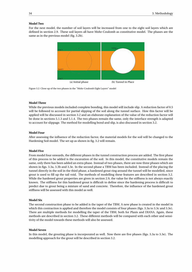
34 3. Methodology
Model Two
For the next model, the number of soil layers will be increased from one to the eight soil layers which aredefined in section 2.9. These soil layers all have Mohr-Coulomb as constitutive model. The phases are thesame as in the previous model (fig. 3.2b).
Clay 2
Clay 2
Sand 3
(a) Initial phase
Lining
(b) Tunnel in Place
Figure 3.2: Close up of the two phases in the "Mohr-Coulomb Eight Layers" model
Model Three
While the previous models included complete bonding, this model will include slip. A reduction factor of 0.5will be followed to account for partial slipping of the soil along the tunnel surface. How this factor will beapplied will be discussed in section 3.2 and an elaborate explanation of the value of the reduction factor willbe done in sections 5.1.3 and 5.1.4. The two phases remain the same, only the interface strength is adaptedto account for slippage. The method for modelling bond and slip, is also discussed in section 3.2.
Model Four
After assessing the influence of the reduction factor, the material models for the soil will be changed to theHardening Soil model. The set up as shown in fig. 3.2 will remain.
Model Five
From model four onwards, the different phases in the tunnel construction process are added. The first phaseof this process to be added is the excavation of the soil. In this model, the constitutive models remain thesame, only there has been added an extra phase. Instead of two phases, there are now three phases which areshown in figs. 3.3a, 3.3b and 3.3e. In the second phase a TBM has been included. Instead of the placing thetunnel directly in the soil in the third phase, a hardened grout ring around the tunnel will be modelled, sincegrout is used to fill up the tail void. The methods of modelling these features are described in section 3.2.While the hardened grout properties are given in section 2.9, the value for the stiffness is not always exactlyknown. The stiffness for this hardened grout is difficult to define since the hardening process is difficult topredict due to grout being a mixture of sand and concrete. Therefore, the influence of the hardened groutstiffness will be assessed with this model as well.
Model Six
The second construction phase to be added is the taper of the TBM. A new phase is created in the model inwhich this contraction is applied and therefore the model consists of four phases (figs. 3.3a to 3.3c and 3.3e).There are multiple methods for modelling the taper of the TBM, both for Plaxis and DIANA. Again, thesemethods are described in section 3.2. These different methods will be compared with each other and sensi-tivity of the model towards these methods will also be assessed.
Model Seven
In this model, the grouting phase is incorporated as well. Now there are five phases (figs. 3.3a to 3.3e). Themodelling approach for the grout will be described in section 3.2.

3.1. Different models 35
Model Eight
After the grouting, the follow carts of the TBM apply a load on the lining. This first follow carts are driving onthe lining itself before some inlay is placed on which the rest of the follow carts are driving. In this model, thefirst couple of carts are modelled since it is expected that they have a larger influence on the internal liningforces than the carts which are driving on a temporary inlay. The phase in which the tunnel is installed willbe replaced by a phase in which the tunnel is installed and has an additional follow cart load (figs. 3.3a to 3.3dand 3.3f). This is partly based on the results of the previous models and will be discussed in section 4.1.8.
Model Nine
In this model, the last and final construction phase will be added to the model so it consists of all the con-struction phases. This final phase is the in-use phase where the load of the metro trains is acting on the inlayof the tunnel. Therefore this model will consist of six phases (figs. 3.3a to 3.3d, 3.3f and 3.3g).
Model Ten
Modelling these different phases leads to unloading and reloading of the soil. Therefore, as a side step, an-other model is created in which the soil models are changed back to Mohr-Coulomb in order to compare theresults again with Hardening Soil. This will show the influence of the additional unloading/reloading stiffnessparameter in the Hardening Soil constitutive model.
Model Eleven
For all the previous models, the lining is assumed to be made out of one ring, while in reality it is made outof segments. In this model, those segments (and thus the joints) are being modelled. All the phases will beincluded as with model nine and the soil will be applied with the Hardening Soil constitutive model. Themethods for creating these segments are discussed in section 3.2. Figure 3.4 shows the location of the joints.The Janssen theory will be applied to these joints.
Joints
Figure 3.4: The lining with the locations of the joints
Model Twelve
The last 2-dimensional model that will be created is including the buildings located at the surface. Multiplebuildings are present at the surface of which one even has multiple levels. The influence of these buildingson the tunnel lining will be assessed in this last model. The phases remain the same, the overal model will beslightly different (fig. 3.5).

36 3. Methodology
Clay 2
Clay 2
Sand 3
(a) Initial phase
TBM
(b) TBM Phase
TBMContraction
(c) Phase with TBM Taper
Grout pressure
(d) Grouting Phase
Hardened groutLining
(e) Phase with the tunnel in place
Hardened groutLining
Follow -cart point loads
(f) Follow-cart phase
Inlay
Train load
(g) In-use phase
Figure 3.3: Close-up schematisation for the different phases that will be applied in the models

3.1. Different models 37
Sand 1
Silt
Clay 1
Sand 2
Sand 3
Sand 4
Clay 2
Clay 3
Building 1 Building 2 Building 3 Building 4
Figure 3.5: Overview of the model with buildings
3.1.2. 3-DimensionalThree types of models are created in 3D. First, the models in which one ring is modelled will be discussedbefore moving on to the two models with multiple rings:
1. Without construction phases2. With construction phases
One-Ring models
In Plaxis, the first three dimensional models that will be created exist out of one compelete ring of one anda half meters wide. This means the soil body has the same horizontal and vertical size as with the two-dimensional models, but is one and a half meters thick, so a thin slice of soil. An schematic view of thismodel is provided in appendix B. The same type of models will be created as the two dimensional modelswith the exception of the follow cart phase, the model with joints and the model with buildings. For the joints,an explanation is given in section 3.3.1. The exclusion of the follow carts and buildings will be discussed insection 5.2.1. These models with one ring will only be created in Plaxis, in section 5.2.1 an explanation isgiven.
Multiple rings without construction phases
After the models with one ring, more extensive models are created with multiple rings. The first is a modelwithout the construction phases as seen in 2D and with the One-ring models. The reason behind not imple-menting the phases will be discussed in section 5.2.1.
Only two phases are included in these models: 1. Initialisation 2. Constructed tunnel. In the last phase,all the different rings are activated and placed at the same time. Between the rings and segments no jointsare applied, thus it will be a monolithic tunnel. This issue on the joints will be discussed in section 3.3.1.
Multiple rings with construction phases
The second model with multiple rings includes the different construction phases. Except for the inlay andfollow cart, this model will have the same construction phases as with the two dimensional and the one-ringmodels. The tunnel itself will consist of multiple rings without any joints. The exclusion of joints will bediscussed in section 3.3.1. The model starts with an initialisation phase. For every phase after, the construc-tion phases will progress through the soil. The TBM will be present on two rings, the same accounts for thegrouting phase. So for the tunnel between not being excavated yet and the lining being constructed are fourphases. This model is only created in Plaxis and the explanation is given in section 5.2.3.

38 3. Methodology
3.2. 2D modelling techniquesWith the different models described, a description of the different features that are applied in the model willbe given in this section for the two dimensional models. First the techniques used in Plaxis will be discussedand after, the techniques in DIANA.
3.2.1. PlaxisIn order to model the construction process of the tunnel as close to reality as possible, multiple aspects haveto be modelled. How these aspects are modelled in Plaxis is discussed in this section. This section will de-scribe the 2D approach, the techniques in 3D will be discussed in section 3.3.1.
SoilFor the soil layers, the borehole tool is used in Plaxis. The top and bottom height of the different layers canbe given and materials assigned to the different layers, so either Hardening Soil materials of Mohr Coulombmaterials. For the first model, only one layer is specified while for all the other models, eight layers are speci-fied with the borehole tool. The height of the hydraulic head can also be set in this tool. The Mohr-Coulombparameters for the first models are converted from the Hardening Soil parameters given in section 2.9.
LiningModelling the tunnel is done through the tunnelling tool in Plaxis. In this tool a circle representing the tunnelis created from the axis location and radius as input. From that ring, plates and a negative interface are cre-ated. For the plates, the "lining" material model is selected which has the properties of the lining as given insection 2.9 and is an elastic, isotropic material. For the negative interface, a thickness of 0.01 m is applied. Inorder to input the stiffness of the concrete, Plaxis demands an axial stiffness, "EA" and a flexural rigidity, "EI".These stiffnesses have been deducted from the Young’s modulus of uncracked concrete. Inputting specificweight of the material is done through entering a force per unit length per unit width. Table 3.1 shows theinput values that have been used. The created negative interface is located on the outside of the tunnel andis used to model the lack of friction. This interface will receive its properties from the surrounding soil.
value unit
Axial stiffness "EA" 1.225e+07 kN/m
Flexural rigidity "EI" 1.250e+05 kN m2/m
Specific weight 8.75 kN/m/m
Pro
per
ties
Poisson’s ratio 0.2 -
Table 3.1: Lining input properties in Plaxis
Bond/slipAn interface is used in order to model relative movement of the lining with respect to the soil. Which meansshearing material at the contact between the lining and the soil may occur. That contact can be somewherebetween rough, so the soil is fully bonding to the lining, or smooth, the soil is slipping along the lining, asdiscussed in section 2.2.4. In Plaxis, the roughness of the interface is given in the material properties of thesurrounding soil by setting a value for the strength reduction factor, "Ri nter ". The behaviour of the interfaceelements is an elastic-plastic model with a Coulomb criterion. When it is elastic, slipping and gapping oroverlapping may occur. Which means relative movement parallel to the interface or displacement perpen-dicular to the interface may occur. The distinction between elastic and plastic behaviour is coming from theCoulomb criterion. With this criterion, a shear stress is calculated for which the interface behaviour remainselastic. When the shear stress on the interface is higher, the interface will behave plastic and thus permanentslip will occur within the interface. The input for the elastic-plastic model and the Coulomb criterion is com-ing from the surrounding soil parameters. By using the strength reduction factor and taking a value belowone, these values can be decreased for the interface. This is done since usually the contact between soil andlining is weaker and more flexible than the soil [12]. The lowest value possible, to reduce most of the strengthand therefore the friction, is 0.01. For modelling "slip" in this research, the strength reduction factor is set at0.5. The strength reduction factor only works when there is an interface created at the lining or the TBM. Theequations used in Plaxis for calculating the interface properties are given by Brinkgreve et al. [12], but are alsodiscussed in section 5.1.4.

3.2. 2D modelling techniques 39
TBM
For the TBM, the same approach as with the lining is followed. So a circle is created in the tunnel tool inPlaxis, this time with a larger diameter than the tunnel but with the axis at the same location. From the circle,plates and a negative interface are created. The negative interface has a thickness of 0.01 m.
TBM taper
The taper of the TBM is modelled by applying a line contraction to the plates. This can be done in the tun-nelling tool. The value for this contraction is "the area loss as a percentage of the total tunnel area" [12]. Witha 9.4 m and 9.35 m as initial and final TBM diameter respectively, the contraction used is 1.06%. This methodis the preferred method by Plaxis for modelling the taper of the TBM.
Another approach of modelling the taper is available however and can be done by creating a stress releaseof the soil surrounding the TBM. This can be achieved by modelling the total excavation but not applying theTBM in the model. Instead, the calculation phase in which this taper is acting is not entirely run. Plaxis canbe forced to terminate early by setting a value for the total multiplier called "
∑Mst ag e ". This total multiplier
is set a 1.0 when the entire calculation phase is to be run. When it is to terminate early, this value can bereduced [12].
Grout
The effects of grouting are modelled by applying a hydraulic pressure in the excavated soil clusters equal tothe properties given in section 2.9. The pressure at the top of the excavation is given by setting the pressureand the reference height. An increment with depth is also given. The value of this depth gradient will beassessed and discussed. This hydraulic pressure results in a radial pressure on the borehole. This approachis not realistic, as discussed in section 2.8.1. However, this is the preferred approach in Plaxis for modellinggrout.
Follow-cart load
As already discussed in section 3.1, the first follow carts are driving directly on the tunnel lining. The otherfollow carts are driving on a temporary elevated platform which leans on the tunnel lining at the same loca-tion as the wheels of the first carts. Therefore the follow carts will be modelled by applying a point load at thelocation where the wheels drive and the elevated platform leans on the lining.
Inlay
For creating the loads during use, a volume is created in the bottom of the tunnel to represent the concreteaggregate. On this volume a line load is set to model the tunnel loads. The most conservative case is assumedwhen two train are passing each other and both axles are at the same points. So the line load will have theload of two train axles divided over the width of the inlay. This leads to a value of -45.5 kN/m/m.
Joints
For the joints, instead of creating a complete circle, eight curves are created, one for each segment. Togetherthe eight curves are a complete circle. For all the curves, plates and negative interfaces are created. Theactual joints are modelled by creating connections between these curves. For these connections, the rotationcan be set fixed, free or as a spring. The joints will modelled as a spring on which the Janssen theory willbe applied that is described in section 2.3.4. Plaxis requires a rotational stiffness as input for the joints. Inorder to apply the Janssen theory, iterations to assess this rotational stiffness are done manually. A startingrotational stiffness is used after which the normal force and bending moment are calculated by Plaxis. Withthese forces, the stiffness of the joints is back calculated by using equations eqs. (2.1) and (2.2). The usedinput stiffness in the joints is changed until it meets the calculated stiffness. This has to be done for everyjoint seperately. An overview of this procedure is given in fig. 3.6.

40 3. Methodology
Low stiff-ness input
Let Plaxiscalculate
lining forces
Acquire liningnormal forceand bendingmoment at
joint location
Increase input stiffness
Decrease input stiffness
Calculatejoint stiffness
accordingto Janssen
theory
Calculatedstiffnessequal toinput?
Is thecalcu-lated
stiffnesshigher or
lower?
stop
no
higher
lower
yes
Figure 3.6: Manual Janssen iteration procedure
BuildingsThe buildings are modelled by the use of plates. These plates have the same stiffness as the lining except forthe weight, that has been put on zero. Instead a line load is applied to the bottom of the building, so at thefoundation depth.
3.2.2. Modelling in DIANAWhile the same construction process is trying to be recreated, not everything is modelled with the sameapproach in both programs. This section will elaborate on the modelling techniques used in DIANA for mod-elling the construction process of a tunnel as close to reality as possible.
SoilThe soil is modelled by creating a rectangular face for each soil layer. After which every soil layer is assignedto a material. These materials have been created beforehand or are created when assigning them to the faces.No property geometries are assigned to the soils. In order to ensure the stresses in the soil are calculated, aglobal dead weight load is assigned to all the soils. This global dead weight load will also be applied on theother features in the model.
Hydraulic headA hydraulic head load is created to model the ground water level. This load requires the shapes on which itacts and the height of the hydraulic head. This approach of assigning the hydraulic head requires the massdensity of the soil to be specified by the dry density and porosity. This can be assigned in the material prop-erties. This load is included in the same load case as the dead weight. From the dry density and the porosity,the pore pressure are calculated in the soil.
LiningThe lining is modelled by creating a circle at the location of the tunnel. This circle is imprinted on the soillayers but the circle is kept. From the faces that have been created by the imprinting, the excavation face willbe created through extraction. This excavation face will be subtracted from the soil. This will create soil layerswith a hole which can be filled by the excavation faces. On the line the material properties are assigned withthe lining properties given in section 2.9, the element geometry is assigned with the thickness of the lining:0.35 m.
Bond/slipOn the face of the lining, and also the TBM, interface elements can be created. However, the lining andTBM are lines in the model. When selecting them for interface, an interface on either side of that line will becreated while only one between the lining/TBM and soil is needed. Therefore the interface is created from theborehole wall. An interface material model can be assigned. A Coulomb-friction criterion is chosen to modelthe friction along the lining and TBM. When assigning the element geometry to this interface, a geometrywith a thickness of 0.01 m is assigned. While it is possible to assign a thickness of zero and this is the casein reality, the interface properties cannot be determined with the guidelines explained below. While Plaxisdetermines the interface properties based on the soil and strength reduction factor itself, in DIANA, theseproperties are required as input:

3.2. 2D modelling techniques 41
• Normal interface stiffness;• Shear interface stiffness;• Cohesion;• Friction angle;• Dilatancy angle
The input properties for the element stiffnesses can be defined with the following guidelines [28]:
Shear stiffness = A2
t
Esoi l
2(1+νsoi l )(3.1)
Normal stiffness = f ·Shear stiffness (3.2)
with:A Reduction factort Interface thicknessEsoi l Young’s modulus of surrounding soilνsoi l Poisson ratio of surrounding soilf Multiplication factor that can vary between 10 and 100.
For the Coulomb-friction input parameters, the following guidelines are followed [28]:
c = A · csoi l (3.3)
t anφ= A · t anφsoi l (3.4)
With csoi l and φsoi l the cohesion and friction angle of the soil respectively.When using the highest values of the surrounding soils for the different properties, the following input is
acquired for a reduction factor of 0.5 and a multiplication factor of 100 as a first assessment of the interface:
value unit
Normal interface stiffness 3.71e+07 kN/m
Shear interface stiffness 3.71e+05 kN/m3
Cohesion 3.2 kN/m2
Friction Angle 17.8 degrees
Pro
per
ties
Dilatancy angle 0 degrees
Table 3.2: Interface input properties in DIANA
TBMThe TBM is modelled in the same way as the lining. A circle is created for the TBM itself and imprinted in thesoils. The faces extracted from the imprinting are the tail void soil clusters. These shapes are subtracted fromthe soil layers again. The material model with the properties of the TBM given in section 2.9 is assigned tothis circle and an element geometry with a thickness of 0.05m is applied.
TBM taperThe first method to model the taper of the TBM is by applying a stress release value. In order to do this, thecalculation phase with the taper does not include the TBM. Instead, the stress release value will be applied tothe TBM. A value of 1.0 means there is no stress release and a value of 0 means there is no support any moreat all.
Assigning a prescribed deformation to the TBM is another way to model the taper. This displacementwill only exist of translational deformations. Functions are created for the deformation in the vertical andhorizontal direction. These functions ensure the prescribed displacement occur at the right location. For thetop and bottom of the TBM, there will be no prescribed displacement in the horizontal direction while at thesides of the TBM, no prescribed displacements occur in the vertical direction. This load will be placed in adifferent load case than the dead weight and hydraulic head.

42 3. Methodology
GroutThe grout is modelled by a line load on the borehole wall. This load coincides with the grout properties givenin section 2.9 by creating functions for the grouting load in both directions. By using these functions it can beassured that the line load becomes a radial load. This load will be placed in a load case with self weight andwill only applied in the phase with grouting.
Follow-cart loadIn DIANA the load of the follow carts will be modelled with the same approach as used in Plaxis.
InlayFor the inlay, an extra element cluster is created within the tunnel, located at the bottom. This cluster is givenan inlay material model, with a high stiffness and a weight. On this inlay, a line load representing weight ofthe metro trains is applied. The properties of the inlay and train load are given in section 2.9. Again, the mostconservative case is taken in which two train pass each other at the modelled lining ring.
JointsIn order to model the joints, the lining is modelled differently as well. A ring with the diameter of the liningis divided into 8 segments by imprinting points on the lining. The points have the location of the joints. Thesegments that have be formed are used to deduct the excavation clusters from the surrounding soil body.While DIANA has the possibility of creating point interfaces, it is not yet possible in DIANA to apply a pointinterface with the Janssen theory. Therefore a rotational spring will be modelled on which the same approachwill be applied as with Plaxis, so the manual Janssen iterations.
BuildingsThe buildings are constructed by creating lines. These lines are imprinted in the soil again. The created areextracted and subtracted from the soil again. A building material model is given to these lines without anyweight. The weight of these buildings is modelled by applying a line load on the bottom plates of the building.
3.3. 3D modelling techniquesSome of the modelling techniques differ little between two and three dimensions, others might be different.This section will discuss the modelling techniques used for the 3D models in Plaxis and DIANA.
3.3.1. PlaxisSoilCreating soil in 3D in Plaxis is equal to that in 2D. The given model size at the start of the project will createthe soil layers given in the borehole tool in three dimensions.
LiningAgain the tunnelling tool in Plaxis is used in order the create the lining. Everything is the same as in 2D exceptfor modelling the length of the tunnel. In the tunnelling tool a ring size can be assigned and the number ofrings can be set as well. Plaxis itself creates the different excavation clusters and the different lining rings.
Bond/slipThis approach is equal to the approach in 2D. In the tunnelling tool a negative interface can be assigned tothe plates. When creating the extra rings, this negative interface is created along every part of lining as well.
TBMThis approach differs from the 2D approach that has been used, but is also available in 2D. In the tunnellingtool a "thick" lining is created. Plaxis creates another circle in the tool at the given "thickness" of the lining.From this circle, plates can be created and a TBM material can be assigned.
TBM taperThe taper is practically created the same, a line contraction is applied to the TBM plates. The contractionvalue also remains the same. However, when modelling the phases, this taper moves through the soil andthe TBM taper is applied over multiple rings. Therefore, Plaxis requires a reference distance for every phasein order to assess how much taper should be applied for that part of TBM plates in that phase. This has tocoincide with the right amount of taper over the total length of the TBM. A good explanation and example isgiven by Brinkgreve et al. [12].

3.3. 3D modelling techniques 43
GroutThe grout will be modelled in the tunnelling tool as a load on the outside circle, the TBM in this case. Whenthe grout should be active, this load should be activated. The TBM does not have to be active in order to doso.
Follow-cart loadFor creating the follow-cart load, a line load can be used. When creating this line load, the begin and end ofthe line is required as input and the loading in three directions. However, when creating the model, the meshneeds to very fine at the location of the line load to make sure it works on nodes. This very fine mesh causesthe model to have a large computational time.
InlayIn order to create an extra soil cluster to account for the inlay, a surface can be made to create a seperationin an existing soil cluster. The same approach as in 2D, but with the third dimension added. However, whenfollowing the height of the inlay as in 2D, the meshing also becomes a problem. The mesh has to be very finein order to accept the location of the inlay and this causes a large computational time.
JointsJoints have to be created in the analysis itself. In order to create the different segments, the same approachcan be applied as in 2D by creating different curves. In the analysis, a connection can be made between thedifferent segments. However, this connection can only set to "fixed" or "free" and no stiffness can be assigned,neither a rotational nor a translational stiffness.
3.3.2. DIANAFor the three dimensional models in DIANA, less modelling techniques will be discussed. An explanation onthis matter will be given in chapter 5.
SoilThe soil in DIANA is modelled by creating a sheet, just like in 2D, but in order to add the third dimension, thesheets are extruded. This will create the solids that represent the soil. A dead load will also be applied in 3D.
Hydraulic headThe hydraulic head is modelled with the same approach as in 2D. A load has to be added on all the shapesthat are influenced by the hydraulic head. A height of the head is required for input again.
LiningThe lining is modelled by creating a circlesheet at the location of the tunnel. This circlesheet is extruded aswell for a length which is equal to the width of the lining ring. After, this ring will be copied five times soa total of six rings has been created. These circle sheets will subtracted from the soil layers and will resultsin an excavation solids and the soil layers. The lining is created by selecting the faces on the outside of theexcavation solids and extract these, creating surfaces. While the material properties are assigned with thelining properties given in section 2.9, the element geometry is assigned with the thickness of the lining: 0.35m. Regular curved shell elements will be used for the lining.
Bond/slipAs with 2D, the interface will be modelled from the face of the soil surrounding the lining. To these elements,an interface material model can be assigned. A Coulomb-friction criterion is chosen to model the frictionalong the lining and TBM. When assigning the element geometry to this interface, a geometry with a thicknessof 0.01 m is assigned. The guidelines and values discussed in section 3.2.2 will be used again. The shearstiffness has to be used twice, for the extra third dimension.
JointsIn 3D, line interfaces can be created between shells in DIANA. These interfaces can be given a material modelwith the Janssen theorem and coulomb friction. DIANA does the iterations regarding the rotational stiffnessof the interface itself.


4Results
This chapter will discuss the results acquired from the different models. Just as with the investigation itself,the results will be discussed in the step-by-step approach. If any differences may occur, the cause of this willbe discussed in chapter 5, which means the results in regard to the research questions will be given in thatchapter. First the results of 2D will be discussed before moving on to 3D.
4.1. 2-Dimensional
4.1.1. Model One
Sand 3 Sand 3
Lining
Figure 4.1: Phases in model one
Figure 4.2 shows the results of the normal forces and the bending moments for Plaxis and DIANA acquiredfrom model one. This model only consists of one soil layer which has a Mohr-Coulomb constitutive model.Very little difference between Plaxis and DIANA is encountered for both the normal force and bending mo-ment for this model as the lines in figs. 4.2a and 4.2b are not differing from each other. There is also littledifference between the maximum and minimum values given in figs. 4.2c and 4.2d.
4.1.2. Model Two
Clay 2
Clay 2
Sand 3
Lining
Figure 4.3: Phases in model two
Figure 4.4 shows the results of the normal forces and the bending moments for Plaxis and DIANA acquiredfrom model two. This model has eight soil layers with a Mohr-Coulomb constitutive model. What accountedfor the model one results, also accounts for these results. The values for both the normal force and bendingmoment are almost equal along the entire lining. The extreme values differ very little as well.
45

46 4. Results
0°
30°
60°
90°
120°
150°
180°
210°
240°
270°
300°
330°
-3000 kN/m
-2500
-2000
-1500
Comparison normal force Model One
DIANA
Plaxis
(a) Normal forces
0°
30°
60°
90°
120°
150°
180°
210°
240°
270°
300°
330°
-500 kN m/m
-250
0
250
500
Comparison bending moment Model One
DIANA
Plaxis
(b) Bending moments
Max Min
[kN/m] [kN/m]
Plaxis -1418 -2788
DIANA -1415 -2800
(c) Extreme values for normal force
Max Min
[kN m/m] [kN m/m]
Plaxis 538.4 -531.8
DIANA 562.7 -544.1
(d) Extreme values for bending moment
Figure 4.2: Results for the normal force and bending moment for model one
0°
30°
60°
90°
120°
150°
180°
210°
240°
270°
300°
330°
-3000 kN/m
-2500
-2000
-1500
Comparison normal force Model Two
DIANA
Plaxis
(a) Normal forces
0°
30°
60°
90°
120°
150°
180°
210°
240°
270°
300°
330°
-500 kN m/m
-250
0
250
500
Comparison bending moment Model Two
DIANA
Plaxis
(b) Bending moments
Max Min
[kN/m] [kN/m]
Plaxis -1457 -2791
DIANA -1447 -2807
(c) Extreme values for normal force
Max Min
[kN m/m] [kN m/m]
Plaxis 603.3 -571.7
DIANA 625.0 -582.8
(d) Extreme values for bending moment
Figure 4.4: Results for the normal force and bending moment for model two.
4.1.3. Model Three
Figure 4.5 shows the results of the normal forces and the bending moments for Plaxis and DIANA acquiredfrom model three. This model has a reduction factor of 0.5 for the interface strength instead of full bonding inthe previous models. From fig. 4.5a it can be seen that the little difference between Plaxis and DIANA occursat the sides of the tunnel. This difference is not that large when looking at fig. 4.5c. For the bending moment,the figure is less clear, but there is a difference which can be seen in table 4.5d. However, this is also a smalldifference.

4.1. 2-Dimensional 47
0°
30°
60°
90°
120°
150°
180°
210°
240°
270°
300°
330° -3000 kN/m
-2500
-2000
-1500
Comparison normal force Model Three
DIANA
Plaxis
(a) Normal forces
0°
30°
60°
90°
120°
150°
180°
210°
240°
270°
300°
330°
-500 kN m/m
-250
0
250
500
Comparison bending moment Model Three
DIANA
Plaxis
(b) Bending moments
Max Min
[kN/m] [kN/m]
Plaxis -1546 -2729
DIANA -1527 -2743
(c) Extreme values for normal force
Max Min
[kN m/m] [kN m/m]
Plaxis 626.2 -597.9
DIANA 632.6 -597.8
(d) Extreme values for bending moment
Figure 4.5: Results for the normal force and bending moment for model three
4.1.4. Model Four
The results for model four are presented in fig. 4.6. This models is a continuation of the previous model,so partial slipping along the lining is present in this model but the material models for the soil have beenchanged. When comparing the figs. 4.6a and 4.6b with the figs. 4.5a and 4.5b, it can be seen that the shapes ofthe different lines are not exactly the same. Compared to model three, the normal forces are approximatelythe same. The difference in bending moment between Plaxis and DIANA has become larger with a HardeningSoil material model for the soils (figs. 4.6b and 4.6d).
0°
30°
60°
90°
120°
150°
180°
210°
240°
270°
300°
330°
-2500
-2000
-1500
Comparison normal force Model Four
DIANA
Plaxis
(a) Normal forces
0°
30°
60°
90°
120°
150°
180°
210°
240°
270°
300°
330°
-400 kN m/m
-200
0
200
400
Comparison bending moment Model Four
DIANA
Plaxis
(b) Bending moments
Max Min
[kN/m] [kN/m]
Plaxis -1604 -2674
DIANA -1623 -2713
(c) Extreme values for normal force
Max Min
[kN m/m] [kN m/m]
Plaxis 482.1 -412.4
DIANA 372.4 -333.8
(d) Extreme values for bending moment
Figure 4.6: Results for the normal force and bending moment for model four

48 4. Results
4.1.5. Model Five
Clay 2
Clay 2
Sand 3
TBM TBMContraction Grout pressure Hardened groutLining Hardened groutLining
Follow -cart point loads
Inlay
Train load
Figure 4.7: Phases in model five
The first construction phase in the process is the excavation phase which is added to create this model. Theresults of the internal forces of the lining are shown in fig. 4.8. When the lining is constructed after the exca-vation phase, the normal forces in the lining are larger for DIANA than for Plaxis at the top and bottom of thetunnel. For the sides of the tunnel it is the opposite: the lining force are larger for Plaxis than for DIANA. Thisis also the case for the bending moments (fig. 4.8b).
0°
30°
60°
90°
120°
150°
180°
210°
240°
270°
300°
330°
-3000 kN/m
-2500
-2000
-1500
Comparison normal force Model Five
DIANA
Plaxis
(a) Normal forces
0°
30°
60°
90°
120°
150°
180°
210°
240°
270°
300°
330°
-400 kN m/m
-200
0
200
400
Comparison bending moment Model Five
DIANA
Plaxis
(b) Bending moments
Max Min
[kN/m] [kN/m]
Plaxis -1461 -2888
DIANA -1439 -2927
(c) Extreme values for normal force
Max Min
[kN m/m] [kN m/m]
Plaxis 424.6 -365.7
DIANA 338.9 -298.5
(d) Extreme values for bending moment
Figure 4.8: Results for the normal force and bending moment for model five
4.1.6. Model Six
Clay 2
Clay 2
Sand 3
TBM TBMContraction Grout pressure Hardened groutLining Hardened groutLining
Follow -cart point loads
Inlay
Train load
Figure 4.9: Phases in model six
In this model, the taper of the TBM, the second construction phase, is included. If the lining is placed afterthe taper of the TBM, the internal forces would have the values as presented in fig. 4.10. As described insection 3.2, the taper of the TBM can be modelled in different ways. For the results presented in fig. 4.10 thetaper has been modelled as a contraction in Plaxis and a stress release in DIANA. The different modellingapproaches and its influence on the internal lining forces are discussed in section 5.1.9. The choice for theapproach that is shown in this section is also explained.

4.1. 2-Dimensional 49
0°
30°
60°
90°
120°
150°
180°
210°
240°
270°
300°
330°
-2250 kN/m
-2000
-1750
-1500
-1250
-1000
Comparison normal force Model Six
with stress release for DIANA
DIANA
Plaxis
(a) Normal forces
0°
30°
60°
90°
120°
150°
180°
210°
240°
270°
300°
330°
-300 kN m/m
-150
0
150
300
Comparison normal force Model Six
with stress release for DIANA
DIANA
Plaxis
(b) Bending moments
Max Min
[kN/m] [kN/m]
Plaxis -974.3 -2218
DIANA -977.6 -2051
(c) Extreme values for normal force
Max Min
[kN m/m] [kN m/m]
Plaxis 316.4 -316.4
DIANA 235.6 -207.0
(d) Extreme values for bending moment
Figure 4.10: Results for the normal force and bending moment for model six
4.1.7. Model Seven
Clay 2
Clay 2
Sand 3
TBM TBMContraction Grout pressure Hardened groutLining Hardened groutLining
Follow -cart point loads
Inlay
Train load
Figure 4.11: Phases in model seven
For model seven, the grouting phase has been added. When the construction process up to installation ofthe lining is conducted, by including the grouting phase, the results presented in fig. 4.12 are acquired. Forboth DIANA and Plaxis, the normal force values approach uniformity along the lining, for DIANA more thanfor Plaxis. This leads to very low bending moments. Since DIANA is more uniform than Plaxis, the bendingmoments in DIANA are lower than in Plaxis as well.
These results of almost uniform normal force and very low bending moment is caused by the drainedanalysis that has been used. More about this and undrained analysis will be discussed in section 5.1.10.
When having model seven with an undrained analysis and a consolidation phase after, the results infig. 4.13 are acquired. The normal forces are not approaching uniformity anymore and thus are the bend-ing moments not approaching zero anymore as well.
4.1.8. Model Eight
Clay 2
Clay 2
Sand 3
TBM TBMContraction Grout pressure Hardened groutLining Hardened groutLining
Follow -cart point loads
Inlay
Train load
Figure 4.14: Phases in model eight
For this model, the follow-carts have been modelled. The consolidation phase has been modelled after thefollow-cart phase and does not include the follow-cart load. The time the follow carts pass the modelledlining ring is very short. Therefore undrained behaviour is applicable for this phase. The results shown infig. 4.15, are the lining internal forces after the consolidation phase.

50 4. Results
0°
30°
60°
90°
120°
150°
180°
210°
240°
270°
300°
330°
-3400 kN/m
-3200
-3000
-2800
Comparison normal force Model Seven
DIANA
Plaxis
(a) Normal forces
0°
30°
60°
90°
120°
150°
180°
210°
240°
270°
300°
330°
-25 kN m/m
-20
-15
-10
-5
0
5
10
Comparison bending moment Model Seven
DIANA
Plaxis
(b) Bending moments
Max Min
[kN/m] [kN/m]
Plaxis -2793 -3265
DIANA -2730 -2843
(c) Extreme values for normal force
Max Min
[kN m/m] [kN m/m]
Plaxis 5.42 -26.58
DIANA 3.60 -5.45
(d) Extreme values for bending moment
Figure 4.12: Results for the normal force and bending moment for model seven
0°
30°
60°
90°
120°
150°
180°
210°
240°
270°
300°
330° -3400 kN/m
-3000
-2600
-2200
Comparison normal force Model Seven undrained
Plaxis
(a) Normal forces
0°
30°
60°
90°
120°
150°
180°
210°
240°
270°
300°
330° -200 kN m/m
-150
-100
-50
0
50
100
150
200
Comparison bending moment Model Seven undrained
Plaxis
(b) Bending moments
Max Min
[kN/m] [kN/m]
Plaxis -2207 -3106
(c) Extreme values for normal force
Max Min
[kN m/m] [kN m/m]
Plaxis 225.5 -183.5
(d) Extreme values for bending moment
Figure 4.13: Results for the normal force and bending moment for undrained model seven

4.1. 2-Dimensional 51
0°
30°
60°
90°
120°
150°
180°
210°
240°
270°
300°
330° -3400 kN/m
-3000
-2600
-2200
Comparison normal force Model Eight
Plaxis
(a) Normal forces
0°
30°
60°
90°
120°
150°
180°
210°
240°
270°
300°
330° -200 kN m/m
-150
-100
-50
0
50
100
150
200
Comparison bending moment Model Eight
Plaxis
(b) Bending moments
Max Min
[kN/m] [kN/m]
Plaxis -2209 -3108
(c) Extreme values for normal force
Max Min
[kN m/m] [kN m/m]
Plaxis 221.5 -183.2
(d) Extreme values for bending moment
Figure 4.15: Results for the normal force and bending moment for undrained model eight
4.1.9. Model Nine
Clay 2
Clay 2
Sand 3
TBM TBMContraction Grout pressure Hardened groutLining Hardened groutLining
Follow -cart point loads
Inlay
Train load
Figure 4.16: Phases in model nine
Finally, the tunnel will be taken into use. The metro train will now be driving through the tunnel in an extraphase. In this model, the consolidation phase has been placed after the follow carts have passed and before itis taken into use. During this consolidation phase, the inlay is already present. When it is in use, the analysisis also undrained. The time for which a train passes the modelled section is very short. Therefore undrainedanalysis suffices for this phase in the construction process. The results presented in fig. 4.17 are acquiredfrom the undrained phase of the train passage. Compared to the previous models, the normal force at thebottom of the tunnel differs. This also results in a lower bending moment at the bottom of the tunnel.
4.1.10. Development throughout construction process
In order to assess which phase is causing changes in the internal lining forces, the extreme values of theseforces have been plotted in figs. 4.18a and 4.18b. The results from Plaxis and DIANA show the same trend forboth the maximum and minimum values. This is the case for the normal force results as well as the bendingmoment results. With regards to the normal force, Plaxis and DIANA differ very little. The different modellingapproaches for the taper have some influence on the minimum value. For the bending moment, it is clearlyvisible that the difference between Plaxis and DIANA is created in model four. This is when the materialmodels are changed from Mohr-Coulomb to Hardening Soil. With regards to the overal trend, it shows thatwhen including more construction phases, the bending moment decreases.

52 4. Results
0°
30°
60°
90°
120°
150°
180°
210°
240°
270°
300°
330°
-3200 kN/m
-3200
-2800
-2600
-2400
-2200
Comparison normal force Model Nine
Plaxis
(a) Normal forces
0°
30°
60°
90°
120°
150°
180°
210°
240°
270°
300°
330°
-200 kN m/m
-150
-100
-50
0
50
100
150
200
Comparison bending moment Model Nine
Plaxis
(b) Bending moments
Max Min
[kN/m] [kN/m]
Plaxis -2229 -3072
(c) Extreme values for normal force
Max Min
[kN m/m] [kN m/m]
Plaxis 211.5 -178.1
(d) Extreme values for bending moment
Figure 4.17: Results for the normal force and bending moment for model nine
One
Tw
o
Thre
e
Fo
ur
Fiv
e
Six
Seven
Eig
ht
Nin
e
-3500
-3000
-2500
-2000
-1500
-1000
-500
Norm
al fo
rce (
kN
/m)
Extreme normal force values for all the phases
Maximum value DIANA
Maximum value Plaxis
Minimum value DIANA
Minimum value Plaxis
(a)
One
Tw
o
Thre
e
Fo
ur
Fiv
e
Six
Seven
Eig
ht
Nin
e
-800
-600
-400
-200
0
200
400
600
800
Bendin
g m
om
ent (k
N m
/m)
Extreme bending moment values for all the phases
Maximum value DIANA
Maximum value Plaxis
Minimum value DIANA
Minimum value Plaxis
(b)
Figure 4.18: Development of the internal lining forces over the complete construction process
While the trend for Plaxis and DIANA have the same shape with regards to the development of the internallining forces, there are some differences. These differences have been plotted as a ratio and a differencein fig. 4.19 for the normal force and bending moment. For the normal force, the ratio between Plaxis andDIANA differs very little throughout the different models since they are almost equal for every model. Onlythe minimum normal force value difference increase with model six. However, when looking at the ratiobetween Plaxis and DIANA, it can be seen that this difference is not very large compared to the total minimumnormal force. The ratio stays below 1.1 which means the difference is less than ten percent. As shown above,the difference in bending moment between Plaxis and DIANA originates in model four, which is the changein material models. From there on, the ratio of the maximum values remains at approximately the same level.As for the minimum values, the ratio changes, because the difference increases, but also because the actualbending moment values decrease, resulting in a higher ratio difference.

4.1. 2-Dimensional 53
One
Tw
o
Th
ree
Fou
r
Fiv
e
Six
0.8
0.9
1
1.1
1.2
1.3
1.4
1.5
1.6
1.7P
laxis
/DIA
NA
ratio
-50
0
50
100
150
200
Pla
xis
-DIA
NA
diffe
rence
Extreme normal force value difference for all phases
Max value ratio
Min value ratio
Max value difference
Min value difference
(a) Normal force
One
Tw
o
Th
ree
Fou
r
Fiv
e
Six
0
0.2
0.4
0.6
0.8
1
1.2
1.4
1.6
Pla
xis
/ D
IAN
A r
atio
-40
-20
0
20
40
60
80
100
120
Pla
xis
-DIA
NA
diffe
rence
Extreme bending moment value difference for all phases
Max value ratio
Min value ratio
Max value difference
Min value difference
(b) Bending moment
Figure 4.19: Ratio and absolute difference between Plaxis and DIANA
4.1.11. Model TenIn order to assess the difference between the Mohr-Coulomb and Hardening Soil material models again, allthe different phases in the construction process have been carried out with Mohr-Coulomb material modelsas well. Figure 4.20 shows the normal force and bending moment for all the models in the constructionprocess with Mohr-Coulomb and Hardening Soil material models.
Fiv
e
Six
Se
ven
Eig
ht
Nin
e
-3500
-3000
-2500
-2000
-1500
-1000
-500
Norm
al fo
rce (
kN
/m)
Extreme normal force values for Hardening Soil and
Mohr-Coulomb material models in Plaxis
Maximum value HS
Maximum value MC
Minimum value HS
Minimum value MC
(a) Normal force
Fiv
e
Six
Se
ven
Eig
ht
Nin
e
-800
-600
-400
-200
0
200
400
600
800
Bendin
g m
om
ent (k
N m
/m)
Extreme bending moment values for Hardening Soil and
Mohr-Coulomb material models in Plaxis
Maximum value HS
Maximum value MC
Minimum value HS
Minimum value MC
(b) Bending moment
Figure 4.20: Lining forces for Hardening Soil and Mohr Coulomb material models for models five to nine
The figures show that for the different models, the normal forces are approximately equal for HardeningSoil and Mohr-Coulomb. The difference in bending moment between Hardening Soil and Mohr-Coulombcould have already been spotted by looking at the results of model three and four (figs. 4.5 and 4.6). It canalso be spotted by looking at the bending moments for all the different models shown in fig. 4.18b. In thesemodels, no excavation phase has been added yet.
The phases in which the soil is excavated and the TBM taper is modelled add to the difference betweenHardening Soil and Mohr-Coulomb. This difference is nullified by the grouting phase which is added in modelseven. The last construction phases with the follow carts and the train load do not lead to a difference betweenHardening Soil and Mohr Coulomb.
4.1.12. Model ElevenThe stiffness for every joint as a results of the manually performed Janssen iteration is shown in fig. 4.21.Almost all the joints are closed and for the joints which are gaping, the stiffness is close to that of a closedjoint.

54 4. Results
2
1
3
4
56
7
8
(a) Joint numbering
Rotational stiffness Open/closed
[kN m/m/rad]
1 1.32e+05 open
2 1.44e+05 closed
3 1.43e+05 open
4 1.44e+05 closed
5 1.44e+05 closed
6 1.44e+05 closed
7 1.44e+05 closed
Join
t
8 1.44e+05 open
(b) Rotational stiffness for each joint
Figure 4.21: Joint numbering and accompanying rotational stiffness
With these stiffnesses for the different joints, the results shown in fig. 4.22 have been acquired.
0°
30°
60°
90°
120°
150°
180°
210°
240°
270°
300°
330°
-3200 kN/m
-3200
-2800
-2600
-2400
-2200
Comparison normal force Model Eleven
Plaxis
(a) Normal forces
0°
30°
60°
90°
120°
150°
180°
210°
240°
270°
300°
330°
-150 kN m/m
-100
-50
0
50
100
150
200
Comparison bending moment Model Eleven
Plaxis
(b) Bending moments
Max Min
[kN/m] [kN/m]
Plaxis -2237 -3071
(c) Extreme values for normal force
Max Min
[kN m/m] [kN m/m]
Plaxis 188.3 -153.5
(d) Extreme values for bending moment
Figure 4.22: Results for the normal force and bending moment for model eleven
4.1.13. Model Twelve
In this model, the buildings have been added. As discussed in section 3.1 the buildings are included after theinitialisation phase and before the tunnel construction commences. The results are shown in fig. 4.23.

4.2. 3-Dimensional 55
0°
30°
60°
90°
120°
150°
180°
210°
240°
270°
300°
330°
-3200 kN/m
-3200
-2800
-2600
-2400
-2200
Comparison normal force Model Twelve
Plaxis
(a) Normal forces
0°
30°
60°
90°
120°
150°
180°
210°
240°
270°
300°
330° -150 kN m/m
-100
-50
0
50
100
150
Comparison bending moment Model Twelve
Plaxis
(b) Bending moments
Max Min
[kN/m] [kN/m]
Plaxis -2270 -3041
(c) Extreme values for normal force
Max Min
[kN m/m] [kN m/m]
Plaxis 164.6 -140.3
(d) Extreme values for bending moment
Figure 4.23: Results for the normal force and bending moment for model twelve
4.2. 3-DimensionalThe results of the three dimensional models will be presented in this section. First the one-ring models inPlaxis will be presented before moving on to the multiple ring models in Plaxis and DIANA.
4.2.1. One-ring modelsWhen comparing the different one-ring models with the two dimensional models, fig. 4.24 is acquired. Theforces over the entire lining for every model in two and three dimensions are attached in appendix I. It canbe seen that the normal forces are almost equal in two and three dimensions for the different constructionphases. The bending moment is almost exactly the same in two and three dimensions.
One
Tw
o
Th
ree
Four
Fiv
e
Six
Seven
Nin
e
Ten
-3500
-3000
-2500
-2000
-1500
-1000
-500
Norm
al fo
rce (
kN
/m)
Extreme normal force values for all the phases
Maximum value 3D
Maximum value 2D
Minimum value 3D
Minimum value 2D
(a)
One
Tw
o
Th
ree
Four
Fiv
e
Six
Seven
Nin
e
Ten
-800
-600
-400
-200
0
200
400
600
800
Bendin
g m
om
ent (k
N m
/m)
Extreme bending moment values for all the phases
Maximum value 3D
Maximum value 2D
Minimum value 3D
Minimum value 2D
(b)
Figure 4.24: Development of the internal lining forces over the different models in 2D and 3D
4.2.2. Without construction phasesWhen not modelling the construction phases or the joints, the results in fig. 4.25 are of a cross section throughring six of the ten ring model in Plaxis and the fourth of six rings in DIANA. The results for Plaxis look verystrange with many peak forces. In order to acquire the results of a ring in 3D, a cross section is made in thecenter of ring six after calculation has been done. This section does not cross every element exactly at a node.Since it is done after the calculation an interpolation between nodes provides the value at the location of the

56 4. Results
cross section. However, these are still interpolated values. This is the cause of the irregular curve, mainly infig. 4.26a. The results for DIANA on the other hand are smoother. While cross sections are easy the create inDIANA, the data from that cross section cannot be exported. Instead, an extra ring is created in the modelbefore the analysis, a so called "composed line". This ring does not have a material assigned and it does notinfluence calculations. It only remembers the structural forces at the location of that "composed line". Thecurve of DIANA in fig. 4.25a looks much like a trendline for the Plaxis curve. This shows that the results areequal, as can been seen with the bending moment as well. The displacements in both programs can be foundin appendix F.
0°
30°
60°
90°
120°
150°
180°
210°
240°
270°
300°
330°
-3000 kN/m
-2500
-2000
-1500
Comparison normal force 3D models without
construction phases
DIANA
Plaxis
(a)
0°
30°
60°
90°
120°
150°
180°
210°
240°
270°
300°
330°
-400 kN m/m
-200
0
200
400
Comparison bending moment 3D models without
construction phases
DIANA
Plaxis
(b)
Figure 4.25: The internal lining forces for the multiple ring models without construction phases
4.2.3. With construction phasesFor the model with ten tunnel rings and the construction phases, the results shown in fig. 4.26 are acquiredin comparison with the two-dimensinal models. These results have been taken from the last ring. Whenconsidering a trendline for the Plaxis curve, it can be seen that the normal force is lower for 3D than for 2D.Because the difference is approximately the same over the entire lining. The bending moment is lower as well,this coincides with the decrease in bending moment in Plaxis for the model without construction phases aswell (section 5.2.2). More will be discussed in section 5.2.3.
0°
30°
60°
90°
120°
150°
180°
210°
240°
270°
300°
330°
-3000 kN/m
-2500
-2000
Comparison normal force for 3D ring model and 2D
with construction phases
3D
2D
(a)
0°
30°
60°
90°
120°
150°
180°
210°
240°
270°
300°
330° -200 kN m/m
-100
0
100
200
Comparison bending moment for 3D ring model and 2D
with construction phases
3D
2D
(b)
Figure 4.26: The internal lining forces for the two and three dimensional models with the construction phases.

5Discussion
In this chapter the results from chapter 4 will be discussed. The differences between the Plaxis and DIANAwill be discussed and some sensitivity analyses as well.
5.1. 2-Dimensional
5.1.1. Model One
As seen in the results, there are very little differences between Plaxis and DIANA. However, the models havenot be validated yet. In order to do so, a analytical approach is used to calculate the maximum normal forceand bending moment in the lining. The calculations based on equations given by COB-L500 [18], Möller andVermeer [66] can be found in appendix D. The results of these calculations are compared with the results fromthe models in table 5.1. Both analytical approaches show a good match with the finite elements models.
Plaxis DIANA Möller and Vermeer [66] COB-L500 [18]
Maximum normal force [kN/m] 2788 2800 2853 2858
Maximum bending moment [kN m/m] 538.4 562.7 557.2 556.3
Table 5.1: Validation of models with extreme values of analytical approach
5.1.2. Model Two
The small difference with the first model is caused by the different soil layers. The overal stiffness of thelayers on top is slightly lower compared to model one. This causes larger displacements and therefore higherbending moments. This would be expected in reality as well.
5.1.3. Interface sensitivity
In Plaxis the interface strength, Ri nter , is a rather arbitrary value. Therefore, its influence is assessed. Fig-ure 5.1 shows the extreme values for the normal force and bending moment results for different values of thisinterface strength. The forces over the entire lining for every reduction factor in Plaxis are given in appendix E,the exact values of the extreme values are also given. Figure 5.1 shows that a decrease in interface strengthleads to less extreme values of normal force in the lining. The maximum and minimum values get closer toeach other with a lower strength.
For the bending moment, the extreme values become more extreme with decreasing strength of the in-terface and therefore the difference between these values increases.
57

58 5. Discussion
0.01
0.05 0.
10.
20.
30.
5 1
Reduction factor (-)
-3000
-2800
-2600
-2400
-2200
-2000
-1800
-1600
-1400
Norm
al fo
rce (
kN
/m)
Extreme normal force values for different reduction factors
Maximum value DIANA
Maximum value Plaxis
Minimum value DIANA
Minimum value Plaxis
(a) Normal force
0.01
0.05 0.
10.
20.
30.
5 1
Reduction factor (-)
-1500
-1000
-500
0
500
1000
1500
Bendin
g m
om
ent (k
N m
/m)
Extreme bending moment values for different reduction factors
Maximum value DIANA
Maximum value Plaxis
Minimum value DIANA
Minimum value Plaxis
(b) Bending moment
Figure 5.1: Lining forces for different reduction factors on interface strength in Plaxis and DIANA
As described in section 3.2.2, DIANA requires input parameters based on a reduction factor for the inter-face strength. To check the influence of this strength, the reduction value has been varied and the extremevalues are also shown in fig. 5.1. The forces along the entire lining for every reduction factor are given inappendix E together with the extreme values.
There is very little difference between the results of the reduction values 1.0 to 0.3. Decreasing the re-duction factor further towards zero, the extreme values for the normal force become less extreme. With de-creasing strength, the difference between the maximum and minimum values for the normal force decreases.The bending moment for the different values of the reduction factor differ very little as well up to 0.1. Whendecreasing further, the bending moment becomes more extreme.
This is the case when a multiplication factor (f) of 100 for determination of the normal force in eq. (5.3) isused. The only influence of this multiplication factor is the normal interface strength. To assess the influenceof this multiplication factor, the values for the normal interface strength are compared. The results for thetwo multiplication factors are compared in fig. 5.2. For a high value for the reduction factor, the results areequal, the same as seen in the results in fig. 5.1. For the lower values, they are almost the same as well. Theonly major difference that occurs is for a reduction factor of 0.01. For this reduction value, the minimumnormal force is higher and this causes the bending moment to increase as well.
0.01
0.05 0.
10.
20.
30.
5 1
Reduction factor (-)
-3000
-2800
-2600
-2400
-2200
-2000
-1800
-1600
-1400
Norm
al fo
rce (
kN
/m)
Extreme normal force values for different reduction factors
Maximum value f=100
Maximum value f=10
Minimum value f=100
Minimum value f=10
(a) Normal force
0.01
0.05 0.
10.
20.
30.
5 1
Reduction factor (-)
-1500
-1000
-500
0
500
1000
1500
Bendin
g m
om
ent (k
N m
/m)
Extreme bending moment values for different reduction factors
Maximum value f=100
Maximum value f=10
Minimum value f=100
Minimum value f=10
(b) Bending moment
Figure 5.2: Lining forces for different reduction factors on interface strength for different multiplication factors in DIANA
Thus, the influence of the interface strength is the same for Plaxis as for DIANA. For the reduction values1.0 - 0.3 has little influence on the internal force of the lining. The lower values of the reduction also show aresemblance. A decrease in interface strength leads to:
• Increase for maximum and decrease for minimum normal force, thus becoming less extreme;• Increase for both maximum and minimum bending moment, thus becoming more extreme;

5.1. 2-Dimensional 59
As discussed in section 2.2.4, a decrease in interface strength leads to less frictional resistance and shearstresses are decreased along the lining as well. This all leads to less support surrounding the tunnel. Thiscauses the bending moment to increase. Which has also been discussed in this section. In reality, it is difficultto assess the actual slippage or loss of friction along the lining. Generally, the friction angle between a walland the soil is 2/3 of the friction angle of the soil. Depending on the smoothness of the wall, this may bedecreased. Figures 5.3 and 5.4 show the stresses in the interface for different values of the reduction factor inPlaxis and DIANA respectively. Decreasing the reduction factor leads to a decrease in interface stresses. Thismeans that plastic displacements along the lining start to occur faster. For a reduction factor of 0.01 there isalmost now shear stress any more. Both the normal stress and shear stress in the interface are alike for Plaxisand DIANA.
0°
30°
60°
90°
120°
150°
180°
210°
240°
270°
300°
330° -800 kN/m
2
-600
-400
-200
0
Normal stresses in interfaces in Plaxis for
different interfaces stiffnesses
R = 1.0
R = 0.5
R = 0.01
(a) Normal stress
0°
30°
60°
90°
120°
150°
180°
210°
240°
270°
300°
330°
-200 kN/m2
-100
0
100
200
Shear stresses in interfaces in Plaxis for
different interfaces stiffnesses
R = 1.0
R = 0.5
R = 0.01
(b) Shear stress
Figure 5.3: Interface stresses for different values of the reduction factor in Plaxis
0°
30°
60°
90°
120°
150°
180°
210°
240°
270°
300°
330° -800 kN/m
2
-600
-400
-200
0
Normal stresses in interfaces in DIANA for
different interfaces stiffnesses
A = 1.0
A = 0.5
A = 0.01
(a) Normal stress
0°
30°
60°
90°
120°
150°
180°
210°
240°
270°
300°
330°
-200 kN/m2
-100
0
100
200
Shear stresses in interfaces in DIANA for
different interfaces stiffnesses
A = 1.0
A = 0.5
A = 0.01
(b) Shear stress
Figure 5.4: Interface stresses for different values of the reduction factor in DIANA
5.1.4. Model ThreeWhen modelling the interfaces and incorporating partial slip, differences may occur between Plaxis and DI-ANA especially for the lower reduction factors as discussed above. The cause of the difference between Plaxisand DIANA will be discussed in this section.
Figure 5.1 shows that the normal force values did not differ greatly between DIANA and Plaxis, which wasalso visible in fig. 4.5a. The same accounts for the bending moment except for a reduction factor of 0.01. Inappendix E the forces over the entire lining of Plaxis and DIANA, of which the extreme values are shown infig. 5.1, are combined.
While for DIANA different input parameters have to be given which can be determined with a reduction

60 5. Discussion
factor, the input in Plaxis is just a reduction factor. Following this reduction factor, Plaxis calculated theinterface strength as follows [12]:
Kn = Eoed ,i
ti(5.1)
Ks = Gi
ti(5.2)
with:Kn Normal stiffness of the interface;Ks Shear stiffness of the interfaceti Interface thickness;Eoed ,i One-dimensional compression modulus of the interface, determined by eq. (5.3);Gi Shear modulus of the interface, determined by eq. (5.4)
Eoed ,i = 2Gi1−νi
1−2νi;νi = 0.45 (5.3)
Gi = R2i nter Gsoi l (5.4)
A value for Gsoil is chosen that corresponds with the stiffness parameters used as input in both Plaxis andDIANA. The thickness interface and reduction factor are the same as chosen for with the DIANA calculation:0.01 m and 0.5 respectively. With Gsoil is 14830 kN/m2, the interface properties become:
value unit
Normal interface stiffness 4.08e+06 kN/m
Shear interface stiffness 3.71e+05 kN/m3
Cohesion 3.2 kN/m2
Friction Angle 17.8 degrees
Pro
per
ties
Dilatancy angle 0 degrees
Table 5.2: Interface properties with the Plaxis calculation
The values shown in table 5.2 differ from the values given in table 3.2. This means there is already adifference in interface strength between Plaxis and DIANA for the same reduction factor. They are closer tothe values for the interface strength with a multiplication factor of ten. Therefore a different value for the lowreduction factor is expected. Figure 5.5 shows the difference between Plaxis and DIANA for the same interfacestrength (table 5.2). A combined figure of the forces in Plaxis and DIANA over the entire lining can be foundin appendix E.
0.01
0.05 0.
10.
20.
30.
5 1
Reduction factor (-)
-3000
-2800
-2600
-2400
-2200
-2000
-1800
-1600
-1400
Norm
al fo
rce (
kN
/m)
Extreme normal force values for different reduction factors
Maximum value DIANA
Maximum value Plaxis
Minimum value DIANA
Minimum value Plaxis
(a) Normal force
0.01
0.05 0.
10.
20.
30.
5 1
Reduction factor (-)
-1500
-1000
-500
0
500
1000
1500
Bendin
g m
om
ent (k
N m
/m)
Extreme bending moment values for different reduction factors
Maximum value DIANA
Maximum value Plaxis
Minimum value DIANA
Minimum value Plaxis
(b) Bending moment
Figure 5.5: Lining forces for different reduction factors with the same input for the interface strength

5.1. 2-Dimensional 61
With no difference in interface strength parameters, Plaxis and DIANA still show some differences. Again,the difference for the normal force and bending moment increases with a decreasing reduction factor. Thedifference for the lowest value of the reduction factor between Plaxis and DIANA is much less than in theprevious case. This is especially visible for the bending moment. For the same input strength for the inter-faces, the difference in extreme values between Plaxis and DIANA is approximately 200 kN m/m. While forthe different interface strength parameters, the difference was approximately 400 kN m/m.
As for the results shown in section 4.1.3, they coincide with what has been discussed in section 5.1.3.Reducing the friction along the lining leads to a higher bending moment. In reality, there is no full frictioneither. With a conservative approach of reducing the friction along the lining by a half, the bending momentsbecome slightly higher and therefore this value seems realistic.
5.1.5. Model FourThe change in soil material models mainly showed a reduction in bending moments. The soil behaves stifferfor unloading with this material models, causing less displacements. Something which is closer to realitythan the Mohr-Coulomb material model, as already discussed in section 2.6.5.
The results presented in section 4.1.4 also include the difference between Plaxis and DIANA caused bythe interface. The difference between the extreme values given in fig. 4.6 are different from the values givenin fig. 4.5. That means there is a difference in the material model definition in Plaxis and DIANA on topof the interface difference. In order remove this little difference the interface is set to full bonding and theresults from those models are shown in fig. 5.7. There is still a difference between Plaxis and DIANA andthis is caused by the material models. In Plaxis, the material model is called "Hardening Soil" which is amaterial model Plaxis created themselves. DIANA has an equivalent of the "Hardening Soil" model called"Modified Mohr-Coulomb". The difference in the results shows that the two material models are not exactlythe same. This can also be seen in the total displacements of this model (fig. 5.6), while there is no differencefor the total displacements in model three appendix F. Figure 5.6 shows that there is less displacement of thesurrounding soil in DIANA, thus with the Modified Mohr-Coulomb material model, the soil is stiffer than withthe Hardening Soil material model in Plaxis. It is difficult to state which of the two is more realistic. Actualproject data has to be used in order to validate both soil models.
(a) Plaxis (b) DIANA
Figure 5.6: Total displacements for model four in Plaxis and DIANA
5.1.6. Mohr-Coulomb vs Hardening SoilTo illustrate the difference in internal lining forces for Mohr-Coulomb and Hardening Soil material modelseven better, figs. 5.8 and 5.9 have been created for Plaxis and DIANA respectively.
For the normal forces in Plaxis (fig. 5.8a), there is little difference between Mohr-Coulomb and HardeningSoil. The reduction factor of the interfaces is more influential. Which is already discussed in section 5.1.3.The reduction factor is also more influential for the bending moments (fig. 5.8b). However, the materialmodels do have a significant influence. Figure 5.8a might be a bit misleading since it seems that the lines fora reduction factor of 0.5 are not that far apart which is caused by the high values on the axis. When looking atthe difference in values between Mohr-Coulomb and Hardening Soil in figs. 5.8d and 5.8f, it can be seen thatthe differences are large. The results, however, for Hardening Soil are more realistic (section 2.6.5).
In DIANA, the material model change seems to have a larger influence on the internal forces of the liningcompared to Plaxis. Similar results were found in section 4.1.4. Especially in fig. 5.9b it is clearly visible where

62 5. Discussion
0°
30°
60°
90°
120°
150°
180°
210°
240°
270°
300°
330°
-3000 kN/m
-2500
-2000
-1500
Comparison normal force model four with full bonding
DIANA
Plaxis
(a) Normal forces
0°
30°
60°
90°
120°
150°
180°
210°
240°
270°
300°
330°
-250
0
250
500
Comparison bending moment model four with full bonding
DIANA
Plaxis
(b) Bending moments
Max Min
[kN/m] [kN/m]
Plaxis -1548 -2758
DIANA -1509 -2783
(c) Extreme values for normal force
Max Min
[kN m/m] [kN m/m]
Plaxis 463.8 -392.7
DIANA 365.0 -316.7
(d) Extreme values for bending moment
Figure 5.7: Results for the normal force and bending moment for model four with full bonding
0°
30°
60°
90°
120°
150°
180°
210°
240°
270°
300°
330°
-3000 kN/m
-2500
-2000
-1500
-1000
Normal Forces for Mohr-Coulomb vs
Hardening Soil in Plaxis
MC - Rinter
= 0.01
HS - Rinter
= 0.01
MC - Rinter
= 0.5
HS - Rinter
= 0.5
MC - Rinter
= 1.0
HS - Rinter
= 1.0
(a) Normal forces
0°
30°
60°
90°
120°
150°
180°
210°
240°
270°
300°
330°
-1000 kN m/m
-500
0
500
1000
Bending Moments for Mohr-Coulomb vs
Hardening Soil in Plaxis
MC - Rinter
= 0.01
HS - Rinter
= 0.01
MC - Rinter
= 0.5
HS - Rinter
= 0.5
MC - Rinter
= 1.0
HS - Rinter
= 1.0
(b) Bending moments
Rinter Max Min
[-] [kN/m] [kN/m]
0.01 -1901 -2482
0.5 -1546 -2723
1.0 -1457 -2791
(c) Extreme values for normal force withMohr-Coulomb material model
Rinter Max Min
[-] [kN m/m] [kN m/m]
0.01 1190 -1170
0.5 614.9 -589.9
1.0 603.3 -571.7
(d) Extreme values for bending moment withMohr-Coulomb material model
Rinter Max Min
[-] [kN/m] [kN/m]
0.01 -1896 -2471
0.5 -1604 -2674
1.0 -1548 -2758
(e) Extreme values for normal force with HardeningSoil material model
Rinter Max Min
[-] [kN m/m] [kN m/m]
0.01 1155 -1149
0.5 482.1 -412.4
1.0 463.8 -392.7
(f) Extreme values for bending moment withHardening Soil material model
Figure 5.8: Results for the normal force and bending moment for the Mohr-Coulomb and Hardening Soil material models in Plaxis

5.1. 2-Dimensional 63
all the Mohr-Coulomb plots are close to each other and the Hardening Soil plots as well. The values for thebending moment for the Hardening Soil material model are almost half of the values for the Mohr-Coulombmaterial model figs. 5.9d and 5.9f. There is even a difference between Mohr-Coulomb and Hardening Soilfor a reduction factor of 0.01 while this is not the case for Plaxis. Since the lining forces differ with the onlydifference between the models are the material models for the soil, the difference between Plaxis and DIANAis caused by these material models. The Modified Mohr-Coulomb/Hardening Soil material model in DIANAis not the same as the Hardening Soil model in Plaxis.
0°
30°
60°
90°
120°
150°
180°
210°
240°
270°
300°
330°
-3000 kN/m
-2500
-2000
-1500
-1000
Normal forces for Mohr-Coulomb vs
Hardening Soil in DIANA
Mohr-Coulomb - A = 0.01
Hardening Soil - A = 0.01
Mohr-Coulomb - A = 0.5
Hardening Soil - A = 0.5
Mohr-Coulomb - A = 1.0
Hardening Soil - A = 1.0
(a) Normal forces
0°
30°
60°
90°
120°
150°
180°
210°
240°
270°
300°
330°
-750 kN m/m
-500
-250
0
250
500
750
Bending moments for Mohr-Coulomb vs
Hardening Soil in DIANA
Mohr-Coulomb - A = 0.01
Hardening Soil - A = 0.01
Mohr-Coulomb - A = 0.5
Hardening Soil - A = 0.5
Mohr-Coulomb - A = 1.0
Hardening Soil - A = 1.0
(b) Bending moments
A Max Min
[-] [kN/m] [kN/m]
0.01 -2015 -2502
0.5 -1491 -2774
1.0 -1447 -2807
(c) Extreme values for normal force withMohr-Coulomb material model
A Max Min
[-] [kN m/m] [kN m/m]
0.01 789.5 -793.9
0.5 626.4 -591.6
1.0 625.0 -582.8
(d) Extreme values for bending moment withMohr-Coulomb material model
A Max Min
[-] [kN/m] [kN/m]
0.01 -1990 -2246
0.5 -1603 -2731
1.0 -1509 -2783
(e) Extreme values for normal force with HardeningSoil material model
A Max Min
[-] [kN m/m] [kN m/m]
0.01 501.0 -521.3
0.5 368.1 -332.0
1.0 365.0 -316.7
(f) Extreme values for bending moment withHardening Soil material model
Figure 5.9: Results for the normal force and bending moment for the Mohr-Coulomb and Hardening Soil material models in DIANA
5.1.7. Model FiveFor this model, the interface stiffness had to be changed to a linear elastic interface with different input pa-rameters in DIANA. This is caused by the hardened grout that is surrounding the lining and it has differentstiffness parameters than the soil. For Plaxis, it automatically takes its interface parameters from the hard-ened grout. In this model a difference for the bending moment is still present. Figure 5.10 shows the phasedisplacements when of the phase in which the TBM is modelled. These displacements seem approximatelythe same in Plaxis and DIANA. The differences in bending moment still originate from the change in materialmodels made in model four.
Including this phase does cause the bending moment to decrease while the normal force becomes moreextreme. The more extreme normal forces are caused by the floating of the TBM. The weight of the TBM islower than the excavated soil and it is non-porous. The pore pressure underneath the tunnel cause the TBMto start floating upwards, which can also be seen in fig. 5.10. It causes the normal force at the top and bottomto be decreased slightly. At the sides, the normal force is slightly increased due to the presence of the hardenedgrout. Since the hardened grout is also stiffer than the soil, it also slightly decreases the bending moment. Inreality this hardened grout is stiffer than soil as well, how much stiffer is not always clear however. Therefore,its influence is discussed in section 5.1.8.

64 5. Discussion
(a) Plaxis (b) DIANA
Figure 5.10: Phase displacement in phase with TBM
5.1.8. Hardened grout stiffness sensitivityIn model five, hardened grout is included. The influence of its stiffness is shown in fig. 5.11. The highestvalue taken for the stiffness of the grout is the stiffness of the weakest construction concrete that is used inthe industry. The lowest value for the stiffness is that of the surrounding soil. It can be seen that for a higherhardened grout stiffness, the internal forces in the lining are reduced. This accounts both for Plaxis and forDIANA and it applies to the normal forces as well as the bending moments. The maximum values for thenormal force are located at the top and bottom of the tunnel while the minimum value are found at the sides.The same accounts for the bending moments. Below a stiffness of 1e+06 kN/m2, the values for the internalforces are approximately the same. When the stiffness becomes higher than 1e+06 kN/m2, the hardenedgrout does not act as transfer medium for forces applied by the soil, but is taking on some of the forces itselfand therefore reducing the forces in the lining. For a high hardened grout stiffness the forces in the liningeven become positive, which means tension. This is all due to the fact that the surrounding grout starts toact as an extra lining. Regardless of the stiffness of the hardened grout, the difference between the bendingmoment in Plaxis and DIANA remains the same (fig. 5.11b). It is decided to take a value of 500e+03 kN/m2
since it seems the most realistic value. This because it is stiffer than soil, as a mixture of soil and concretewould be, and it only has a slight influence on the lining forces for which most of it is transferred to the liningitself.
50e+
03
100e
+03
500+
e03
1+e0
6
5+e0
6
10+e
06
25e+
06
Hardened Grout Stiffness (kN/m2)
-3500
-3000
-2500
-2000
-1500
-1000
-500
0
500
1000
Norm
al fo
rce (
kN
/m)
Extreme normal force values for different hardened grout stiffness
Maximum value DIANA
Maximum value Plaxis
Minimum value DIANA
Minimum value Plaxis
(a) Normal force
50e+
03
100e
+03
500+
e03
1+e0
6
5+e0
6
10+e
06
25e+
06
Hardened Grout Stiffness (kN/m2)
-500
-400
-300
-200
-100
0
100
200
300
400
500
Bendin
g m
om
ent (k
N m
/m)
Extreme bending moment values for different hardened grout stiffness
Maximum value DIANA
Maximum value Plaxis
Minimum value DIANA
Minimum value Plaxis
(b) Bending moment
Figure 5.11: Lining forces for different values of the hardened grout stiffness
5.1.9. Model SixIn model six, the taper of the TBM is modelled. Realistically, taper leads to a stress release in the surroudingsoil and thus resulting in a decrease in normal force. This is also seen in the results. The decrease in nor-mal force in turn leads to a decrease in bending moment. However, in reality this amount of displacement,and therefore stress release, will probably not be acquired. Between the shield and the soil already flows liq-uid grout which comes from the back of the TBM. This already puts a pressure on the surrounding soil andtherefore decreases the stress release of the soil.

5.1. 2-Dimensional 65
This taper can be modelled in multiple ways as described in section 3.2. The results shown in section 4.1.6are conducted with a stress release in DIANA and an applied contraction in Plaxis. A prescribed deformationcan also be applied in DIANA. The advantage of prescribed deformation approach in DIANA and contractionapproach in Plaxis is that the TBM remains active during modelling. This incorporates the weight of the TBMin the model. Therefore these two approaches will be assessed first. The phase displacements of the soilalong the lining in which the taper is modelled are shown in fig. 5.12.
(a) Plaxis (b) DIANA
Figure 5.12: Phase displacement in the taper phase for contraction in Plaxis and prescribed deformation in DIANA
When modelling the taper in DIANA, the prescribed deformation ensure the TBM nodes on which thedeformation is applied, move radially with the provided value. Therefore, the entire TBM moves inwardsradially with a fixed axis. Within Plaxis, the contraction of the lining does not cause the soil around the TBMto move radially inward with a fixed axis. Plaxis ensures that the TBM diameter is decreasing, but it does notensure that the axis is fixed. It is letting the TBM move while it is contracting. For DIANA, it can be seenthat the soil moves towards the axis, it seems like the TBM is not allowed to move during the taper. With thisapproach, its advantage of an active TBM is also cancelled.
When applying a line contraction in Plaxis, it will decrease the element size, which in this case are plates.These plates will become smaller because of this line contraction. Be applying a specific value, as describedin section 3.2, of this plate element contraction on all the TBM elements, the taper of the TBM is emulated.
The other approach of modelling the TBM taper, described in section 3.2, is investigated in order to see ifthose results are different. Figure 5.13 shows the results of stress release approach in Plaxis and DIANA. Forthese results, a stress release value is chosen for which the displacement in the borehole are equal to the taperamount of the TBM.
(a) Plaxis (b) DIANA
Figure 5.13: Phase displacement in the taper phase for stress release in Plaxis and DIANA
When assessing the influence of the stress release in both Plaxis and DIANA, fig. 5.15 is acquired. For anMstage value of 0.15 in Plaxis the internal lining forces are the closest to the internal lining forces acquiredwith applying contraction. However, this is not the case with the displacement, the displacements at thetop and bottom combined are only make up for half the displacement with contraction (2.8 cm against 5cm). When Mstage is taken 0.28 approximately the displacement at top and bottom combined equal 5 cm.However, the division between top and bottom is different than when contraction is applied and the internal

66 5. Discussion
lining forces are slightly different as well. Figure 5.15 does show that the displacement at the bottom of theborehole is less than at the top, this accounts both for DIANA and Plaxis. This strengthens the contractionapproach used by Plaxis in which the same phenomena was seen (fig. 5.12). For DIANA, the phase factorfor modelling the stress should be taken 0.66. For this value the borehole has a combined radial inwarddisplacement of 5 cm.
0.05
/0.9
5
0.1/
0.9
0.15
/0.8
5
0.2/
0.8
0.25
/0.7
5
0.3/
0.7
0.35
/0.6
5
0.4/
0.6
0.45
/0.5
5
0.5/
0.5
0.55
,/0.4
5
0.6/
0.4
0.65
/0.3
5
0.7/
0.3
0.75
/0.2
5
MStage (Plaxis) / Phase Factor (DIANA) repectively
-3000
-2500
-2000
-1500
-1000
-500
0
Norm
al fo
rce (
kN
/m)
Extreme normal force values for different stress release values
Maximum value DIANA
Maximum value Plaxis
Minimum value DIANA
Minimum value Plaxis
(a) Normal force
0.05
/0.9
5
0.1/
0.9
0.15
/0.8
5
0.2/
0.8
0.25
/0.7
5
0.3/
0.7
0.35
/0.6
5
0.4/
0.6
0.45
/0.5
5
0.5/
0.5
0.55
/0.4
5
0.6/
0.4
0.65
/0.3
5
0.7/
0.3
0.75
/0.2
5
MStage (Plaxis) / Phase Factor (DIANA) repectively
-400
-300
-200
-100
0
100
200
300
400
Bendin
g m
om
ent (k
N m
/m)
Extreme bending moment values for different stress release values
Maximum value DIANA
Maximum value Plaxis
Minimum value DIANA
Minimum value Plaxis
(b) Bending moment
Figure 5.14: Lining forces for different values of the stress release
0.05
/0.9
5
0.1/
0.9
0.15
/0.8
5
0.2/
0.8
0.25
/0.7
5
0.3/
0.7
0.35
/0.6
5
0.4/
0.6
0.45
/0.5
5
0.5/
0.5
0.55
,/0.4
5
0.6/
0.4
0.65
/0.3
5
0.7/
0.3
0.75
/0.2
5
MStage (Plaxis) / Phase Factor (DIANA) repectively
-0.05
-0.025
0
0.025
0.05
0.075
0.1
0.125
0.15
0.175
0.2
Dis
pla
cem
ent (m
)
Displacement at top and bottom of borehole for different stress release values
Top DIANA
Top Plaxis
Bottom DIANA
Bottom Plaxis
Top+Bottom DIANA
Top+Bottom Plaxis
Figure 5.15: Displacement for top and bottom of the borehole for different stress releases
Which approach is more realistic depends on how the TBM is expected to behave in the soil. If assumedthat the TBM axis is always equal to the tunnel axis, so the TBM is "floating" in the borehole (fig. 5.16a), theprescribed deformation approach in DIANA would be more realistic. If the TBM would behave by "lying"in the borehole (fig. 5.16b), the approach by contraction in Plaxis would be more realistic. For this case, thecontraction approach in Plaxis and thus the stress release approach in DIANA have been chosen as suitablefor modelling the taper of the TBM. The small difference in minimum normal force is caused by a differencein displacements on the sides of the tunnel. When comparing figs. 5.12a and 5.13b, it can be seen that the dis-placements on the side of the tunnel are different. Directly next to the tunnel lining they are of approximatelyequal values, but further way the difference becomes larger. For Plaxis the displacements increase slightlywhen moving away horizontally from the tunnel lining. For DIANA, the displacments stay approximately thesame. In Plaxis the displacements reach a value of approximately one centimeter while DIANA stays at ap-proximately three millimeters. In section 5.1.5 it was discussed that the soil behaves stiffer in the modifiedMohr-Coulomb model than the Hardening Soil in Plaxis, this also causes the difference in displacements onthe sides of the tunnel in this model. Which in turn leads to additional differences in lining forces.

5.1. 2-Dimensional 67
BoreholeTBM
Tunnel/TBM axis
(a) "Floating"
BoreholeTBM
Tunnel axis
TBM axis
(b) "Lying"
Figure 5.16: Exaggeration of possible TBM behaviour in borehole
5.1.10. Model SevenThe almost equal normal forces and the close to zero bending moments are different from the previous mod-els. This is caused by the type of analysis chosen for these models, namely: drained. Drained analysis is usedfor long term behaviour of the soil. In the construction process of a bored tunnel, the phases for the construc-tion are relatively short. When loading a soil in a short period of time, excess pore pressures develop sincethere has not been enough time yet for the pore pressure to dissipate. When using a drained analysis, theseexcess pore pressure are not developed since it already assumed these will dissipate, this causes the soil skele-ton to take on all the forces in order to reach an equilibrium. When modelling it with undrained behaviour,a consolidation phase has to be added in order for these pore pressure to dissipate. The comparison of theinternal forces for drained and undrained behaviour in Plaxis is shown in fig. 5.17.
One
Tw
o
Thre
e
Fo
ur
Fiv
e
Six
Seven
-3500
-3000
-2500
-2000
-1500
-1000
-500
Norm
al fo
rce (
kN
/m)
Extreme normal force values for drained-undrained comparison in Plaxis
Maximum value Plaxis Undrained
Maximum value Plaxis Drained
Minimum value Plaxis Undrained
Minimum value Plaxis Drained
(a) Normal force
One
Tw
o
Thre
e
Fo
ur
Fiv
e
Six
Seven
-800
-600
-400
-200
0
200
400
600
800
Bendin
g m
om
ent (k
N m
/m)
Extreme bending moment values for drained-undrained comparison in Plaxis
Maximum value Plaxis Undrained
Maximum value Plaxis Drained
Minimum value Plaxis Undrained
Minimum value Plaxis Drained
(b) Bending moment
Figure 5.17: Lining forces for drained and undrained analysis in Plaxis for different models
Figure 5.17 shows that for the first six models, there is very little difference between drained or undrainedmodelling in Plaxis. In model seven the difference occurs between drained and undrained. In model seven, agrout pressure is applied. This grout pressure is the first load that causes a compression of the soil comparedto all the other models where there is only relaxation of the soil. This load causes excess pore pressure in thesoil surrounding the borehole, since it is undrained. These pore pressures take on a part of the grout load thatis applied. When consolidation is allowed after, the excess pore pressure are allowed to dissipate and transferthe load it took on to the soil skeleton. This has to come in an equilibrium again. This leads to an increase innormal forces on the lining which in turn leads to higher bending moments.
These higher bending moments are of a more realistic value and therefore from this model onward,undrained analysis will be used instead of drained analysis. These values are also realistic when comparedto the previous models. The grouting pressure puts a force on the borehole, which creates a displacementcontrary to the taper phase. This reloaded soil wants to unload again after the grouting phase causing the in-crease in normal forces. The less stiff locations of the soil along the lining are displaced more, causing a moreuniform unloading after the grouting phase. This leads to a decrease in bending moment. In reality, a grout-ing pressure is also put on the borehole. The exact pressure it puts on every location on the borehole remainsunclear. As discussed in section 2.8.1, the behaviour of the grout is complex. The constant gradient appliedin this research is not realistic. However, its influence on the model has been assessed in section 5.1.11.

68 5. Discussion
As shown in fig. 5.17, there is no need in redoing the previous model undrained since there is little differ-ence for those models between drained and undrained.
For DIANA, undrained analysis is also possible. However, consolidation for the excessive pore pressure todissipate is not yet possible in the current version. Currently DIANA itself uses a workaround which includesuse of a developers version. However, it is not proven yet that the workaround produces results which aretrustworthy. As described above, modelling consolidation is important for the construction process of a boredtunnel. Since this is not possible in DIANA, further research in DIANA will not be possible.
5.1.11. Grout pressure increment sensitivity
The grout pressure applied on the borehole in model seven has an increment over depth. The exact behaviourof the grout is very complex (section 2.8.1). It has been assumed the grout has a constant vertical gradientover depth. In order to assess the influence of this gradient, different values have been taken from a very lowvalue of 6 to 21 kN/m2/m, with the latter equal to the specific weight of the grout.
6 8 10 12 14 16 18 20 22
Grout pressure increment (kN/m2/m)
-3400
-3200
-3000
-2800
-2600
-2400
-2200
Norm
al fo
rce (
kN
/m)
Extreme normal force values for different grout increment values
Maximum value Plaxis
Minimum value Plaxis
(a) Normal force
6 8 10 12 14 16 18 20 22
Grout pressure increment (kN/m2/m)
-200
-150
-100
-50
0
50
100
150
200
250
Bendin
g m
om
ent (k
N m
/m)
Extreme bending moment values for different grout increment values
Maximum value Plaxis
Minimum value Plaxis
(b) Bending moment
Figure 5.18: Lining forces for different values of the vertical grout pressure gradient
It can be seen that for an increase in grouting pressure increment, the normal forces in the lining willincrease as well. The bending moment decreases with an increasing grout pressure gradient. The difference,however, between 6 and 21 kN/m2/m is not that large for both the normal force and bending moment. Sincethe behaviour of grout is complex, the most conservative approach will be used from now on, so a value of 6kN/m2/m will be used as value for the increment of the grout pressure over depth.
5.1.12. Model Eight
There is little difference between model eight and seven. This is caused by the approach of the follow carts.In reality, they are only present for a short period of time and are therefore modelled undrained. After, theconsolidation is applied again in which the follow cart load is not present. The follow cart load has littleinfluence on the long term internal lining forces. During the passage of the follow carts, they do have quitean influence on the bending moment (fig. 5.19). However, the peak bending moment that is caused by thefollow carts is much smaller than bending moments when consolidation has taken place. These peak bendingmoments are not realistic. While there will be a local increase in bending moment, the peak is too sharp. Inreality the follow-carts are driving on a rails, which already distributes the load. The lining itself will alsodistributed some of the load over its thickness. The peak will therefore be more blunt in reality. For the forcesof the lining in the follow-cart phase, DIANA has been added since this is still before a consolidation phaseand therefore possible to model. However, the differences between Plaxis and DIANA are very small.
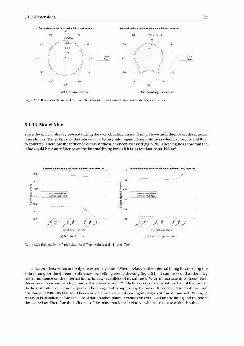
5.1. 2-Dimensional 69
0°
30°
60°
90°
120°
150°
180°
210°
240°
270°
300°
330°
-3000 kN/m
-2500
-2000
-1500
-1000
Comparison normal force during follow cart passage
DIANA
Plaxis
(a) Normal forces
0°
30°
60°
90°
120°
150°
180°
210°
240°
270°
300°
330°
-100 kN m/m
-50
0
50
Comparison bending moment during follow cart passage
DIANA
Plaxis
(b) Bending moments
Figure 5.19: Results for the normal force and bending moment for two follow cart modelling approaches
5.1.13. Model Nine
Since the inlay is already present during the consolidation phase, it might have an influence on the internallining forces. The stiffness of this inlay is an arbitrary value again. It has a stiffness which is closer to soil thanto concrete. Therefore the influence of this stiffness has been assessed (fig. 5.20). These figures show that theinlay would have an influence on the internal lining forces if it is larger than 2e+06 kN/m2.
50e+
03
100e
+03
500+
e03
1+e0
6
5+e0
6
10+e
06
25e+
06
Inlay Stiffness (kN/m2)
-3400
-3200
-3000
-2800
-2600
-2400
-2200
Norm
al fo
rce (
kN
/m)
Extreme normal force values for different inlay stiffness
Maximum value Plaxis
Minimum value Plaxis
(a) Normal force
50e+
03
100e
+03
500+
e03
1+e0
6
5+e0
6
10+e
06
25e+
06
Inlay Stiffness (kN/m2)
100
200
300
-200
-100
0
Bendin
g m
om
ent (k
N m
/m)
Extreme bending moment values for different inlay stiffness
Maximum value Plaxis
Minimum value Plaxis
(b) Bending moment
Figure 5.20: Extreme lining force values for different values of the inlay stiffness
However, these value are only the extreme values. When looking at the internal lining forces along theentire lining for the different stiffnesses, something else is showing (fig. 5.21). It can be seen that the inlayhas an influence on the internal lining forces, regardless of its stiffness. With an increase in stiffness, boththe normal force and bending moment increase as well. While this occurs for the bottom half of the tunnel,the largest influence is on the part of the lining that is supporting the inlay. It is decided to continue witha stiffness of 200e+05 kN/m2. This values is chosen since it is a slightly higher stiffness than soil. When, inreality, it is installed before the consolidation takes place, it creates an extra load on the lining and thereforethe soil below. Therefore the influence of the inlay should be included, which is the case with this value.

70 5. Discussion
0°
30°
60°
90°
120°
150°
180°
210°
240°
270°
300°
330°
-3500 kN/m
-3000
-2500
Normal force for different values
of the inlay stiffness in Plaxis
50e+03
100e+03
200e+03
500e+03
1e+06
2e+06
5e+06
10e+06
20e+06
(a) Normal force
0°
30°
60°
90°
120°
150°
180°
210°
240°
270°
300°
330° -200 kN m/m
-100
0
100
200
Bending moment for different values
of the inlay stiffness in Plaxis
50e+03
100e+03
200e+03
500e+03
1e+06
2e+06
5e+06
10e+06
20e+06
(b) Bending moment
Figure 5.21: Lining forces in the tunnel lining for different values of the inlay stiffness
So the difference with model nine and and the previous models is the inlay during the consolidationphase. What becomes clear is that the actual usage of the tunnel has very little influence on the internallining forces. The passage of the metro train only works for a short period of time in which it is not exerting asignificant force on the lining. Something for which a tunnel is designed in reality as well.
5.1.14. Model Ten
The largest difference between Mohr-Coulomb and Hardening Soil material models was seen in model six.This model included the taper of the TBM, which leads to stress release in the soil surrounding the borehole.More than other phases within the construction process of a bored tunnel. This is where the difference bew-teen Mohr-Coulomb and Hardening Soil material models comes forward really well. In Mohr-Coulomb onevalue is given for different stiffnesses, so the primary loading stiffness is equal to the unloading stiffness andthe reloading stiffness as well. With the Hardening Soil material models, however, different stiffness valuesare used, as described in section section 2.6 and the value for unloading stiffness is higher than the stiffnessused in the Mohr-Coulomb material model. Therefore less loading of the soil on the lining takes place withthe Hardening Soil material models than with the Mohr-Coulomb. In the grouting phase, the internal liningforce become almost equal again for Mohr-Coulomb and Hardening Soil. This is also caused by the differ-ence in defining the stiffness. The reloading stiffness in Hardening Soil is equal to the unloading stiffness andthus larger than the stiffness applied with the Mohr-Coulomb materials model. This can be seen in fig. 5.22which shows the phase displacements for the grouting phase with Hardening Soil and Mohr-Coulomb mate-rial models. The displacements along the borehole are much larger for Mohr-Coulomb than for HardeniningSoil. The grout load in both cases is equal but due to the different reloading stiffness, the deformations differ.However, since the loading is the same for both cases, the soil exerts the same load on the lining when it isinstalled. This causes the difference between Hardening Soil and Mohr-Coulomb to be nullified. Again, thephases with the follow-cart and inlay load have little influence on the final internal lining forces.

5.1. 2-Dimensional 71
(a) Hardening Soil (b) Mohr-Coulomb
Figure 5.22: Phase displacement in the grouting phase for Hardening Soil and Mohr-Coulomb material models in Plaxis
When the material models do not have an influence on the lining forces when the grouting is modelledas a load on the borehole, one can argue what would happen to the difference between Plaxis and DIANAthat is caused by the difference in material models. If the soil actually does exert the same amount of force ashas been placed on the borehole, the difference between Plaxis and DIANA will also be nullified. After whichnew differences may arise due to modelling of the joints or other causes. Unfortunately, it was not possibleto include this in the research as previously explained.
5.1.15. Model ElevenThe small irregularities in the curves that are presented in section 4.1.12, are caused by the joints. Thesejoints have some influence on the internal lining forces. The influence seems to be small since no peaks oflow bending moments are found at the joint locations. However, the bending moment along the entire lininghas been decreased due to these joints and it therefore does has some influence on the internal lining forces.This would also be the case in reality which was also discussed in section 2.5.
5.1.16. Model TwelveThe presence of buildings at the surface leads to a decrease in bending moment. The normal forces differ littlecompared to model eleven, but the difference in bending moment is larger. The joints cause the irregularitiesalong the curves again.
5.1.17. Last modelsWhen plotting the extreme values of models seven to twelve, fig. 5.23 is acquired. It shows that includingmore tunnel features in the model leads to a decrease in bending moments. In model ten all the phaseswere modelled with Mohr-Coulomb material models for the soil layers, this explains the inconsistency in themaximum normal force and minimum bending moment curves.
Seven
Eig
ht
Nin
e
Ten
Ele
ven
Tw
elv
e
-3200
-3100
-3000
-2900
-2800
-2700
-2600
-2500
-2400
-2300
-2200
-2100
Norm
al fo
rce (
kN
/m)
Extreme normal force values for model seven to twelve
Maximum value Plaxis
Minimum value Plaxis
(a) Normal force
Seven
Eig
ht
Nin
e
Ten
Ele
ven
Tw
elv
e
-300
-200
-100
0
100
200
300
Bendin
g m
om
ent (k
N m
/m)
Extreme bending moment values for models seven to twelve
Maximum value Plaxis
Minimum value Plaxis
(b) Bending moment
Figure 5.23: Extreme lining force values for models seven to twelve

72 5. Discussion
In order to assess whether the construction phases also have a positive influence on the combinationof normal force and bending moment, moment-curvature relations have been investigated. The differentNM-κ diagrams for all the models can be found in appendix H, in which a brief description of the graphs isgiven as well. An elaborate explanation and the calculations that form the base of this type of diagrams isgiven by Walraven [80]. The reinforcement is based on model four and is kept the same for all the models. Inappendix H a brief explanation is given on how this is done. The reinforcement is kept the same since onlythe influence of the different construction phases is assessed.
With these moment-curvature relations, unity checks are also done. This is a ratio between the actingbending moment and the bending moment capacity of the lining. More on this is discussed in appendix H.When comparing the unity check for the different models, fig. 5.24 is acquired. It shows that the unity check isdecreased when more construction features are included. Which means the difference between the capacityand acting moment becomes larger in favor of the capacity.
On
e
Tw
o
Th
ree
Fo
ur
Fiv
e
Six
Se
ve
n
Eig
ht
Nin
e
Te
n
Ele
ve
n
Tw
elv
e
Model
0
0.2
0.4
0.6
0.8
1
1.2
1.4
Un
ity c
he
ck (
-)
Unity check for the 2D models in Plaxis and DIANA
Plaxis
DIANA
Figure 5.24: Unity check for all the models in 2D
5.2. 3-Dimensional5.2.1. One-ring modelsThe one-ring models have only been created in Plaxis since it was possible to model all the different construc-tion phases. This is not case in DIANA as explained in section 5.1.10 since consolidation is not yet applicablein the current version of DIANA.
The results in section 4.2.1 show little or no difference between the two dimensional models and the mod-els with one ring. This was expected since the models are almost equal. What has been done with the threedimensional modelling is almost a plane strain approach which has been applied in the two dimensionalmodels. Since it is only one ring and the model is not allowed to move in the direction of the tunnel axis, ittends to go towards a plane strain situation in which the model is supposedly of infinite length.
The phase with the follow-carts has been excluded due to meshing problems. As previously discussed insection 3.3.1 the very fine mesh which is needed for the analysis leads to a large computational time. Whenconsidering that the same results are acquired for these one-ring models as with 2D, it can be assumed thatthe follow carts will have the same influence in this model as in 3D, which is very little. Therefore it has beendecided to no include this phase.

5.2. 3-Dimensional 73
The same meshing problem occured when creating an inlay which is slightly smaller the clay soil clusterin the bottom of the tunnel. Due to the small difference between these two cluster, meshing was not possiblefor anything but the finest mesh. This also lead to a model with a large computational time. It was alreadyconcluded in the two dimensional models that the inlay does have some influence, but it is not very large.Therefore it has been decided to model the soil cluster as the inlay. It is assumed this increase in inlay volumeis of little influence compared to the two dimensional models. The volume with this approach becomes onecubic meter larger per ring which is approximately an increase of seven percent.
5.2.2. Without construction phases
Described in section 3.3.1, the joints cannot be applied in the three dimensional version of Plaxis and aretherefore not included in these models.
While it was expected that difference between Plaxis and DIANA would not be that large, this small wasnot expected either. Without the construction process both models have a monolithic tunnel and only twophases, therefore not a very realistic model. However, the difference between the two models is the materialmodel for the soil. In Plaxis, the Hardening Hoil material model is applied and in DIANA Modified Mohr-Coulomb. In 2D, this caused the difference between Plaxis and DIANA. Figure 5.25 shows the curves formodel four and the 3D model with multiple rings in DIANA. It shows that for the three dimensional modelthe bending moments are higher, this strokes with the results presented in sections 4.1.4 and 4.2.3. Whenlooking at the difference between 2D and 3D in Plaxis (fig. 5.26), the opposite can be seen. The bendingmoment in 3D is slightly smaller than in 2D. Combine this and the increase in bending moment in DIANAfrom 2D to 3D and the difference in 2D between DIANA and Plaxis disappears. Where this differences comefrom has not been found, it does show that for 3D, Modified Mohr-Coulomb and Hardening Soil are moreequal than in 2D. It seems the 2D Modified Mohr-Coulomb is an underestimation of the material model in3D. For Plaxis the Hardening Soil 2D is an overestimated approach of the 3D Hardening Soil. Furthermore, italso seems the difference between DIANA 2D and 3D is less than with Plaxis. Not enough research has beenconducted in order to conclude that for 3D the material models are equal and it might also be a coincidencethere are coinciding like this.
0°
30°
60°
90°
120°
150°
180°
210°
240°
270°
300°
330°
-2500
-2000
-1500
Comparison normal force 2D and 3D DIANA
3D
2D
(a)
0°
30°
60°
90°
120°
150°
180°
210°
240°
270°
300°
330°
-400 kN m/m
-200
0
200
400
Comparison bending moment 2D and 3D DIANA
3D
2D
(b)
Figure 5.25: The internal lining forces for model four and the 3D model in DIANA

74 5. Discussion
0°
30°
60°
90°
120°
150°
180°
210°
240°
270°
300°
330°
-3000 kN/m
-2500
-2000
-1500
Comparison normal force 3D ring model and 2D
without construction phases
3D
2D
(a)
0°
30°
60°
90°
120°
150°
180°
210°
240°
270°
300°
330°
-400 kN m/m
-200
0
200
400
Comparison bending moment for 3D ring model and 2D
without construction phases
3D
2D
(b)
Figure 5.26: The internal lining forces for model four and the 3D model in Plaxis
5.2.3. With construction phasesAs described in section 3.3.1, it is not possible to apply a stiffness to the joints, the only options are free orfixed. Therefore the joints will not be applied in this model and the tunnel will be monolithic. As alreadydescribed in section 5.1.10, the construction phases cannot be implemented in its entirety in DIANA andtherefore will not be included. Thus this model is only created in Plaxis.
Figure 4.26 shows a difference for the normal force between 2D and 3D when modelling multiple rings andthe construction process. As explained, the cross section is taken at the middle. Unlike the model in whichthe construction phases are not modelled, the normal force is not uniform over the ring along the tunnelaxis. The front part of the ring, which gets attached to an already installed ring, has a lower normal forcealong the entire lining than the back part, this is shown in fig. 5.27. It is caused by the modelling sequenceof the rings. When a new ring is installed, the front is attached to another ring. Since the first ring alreadyhad some deformation, one side of the new ring is deformed during installation in order to connect to theprevious ring. This reduces the normal forces in that part of the ring. The back side, which is "free" does nothave this deformation and therefore has more realistic values for the normal force. Figure 5.28a shows thebending moment in the longitudinal direction which shows that the front is deformed as well and the backis not and therefore creating the bending moments. This is the case when the front of the model (YMin) isonly fixed in the normal direction, so in the direction of the tunnel. This means it can move vertically, whathappens when modelling the first ring. With installation of the other rings, the entire tunnel becomes morestable and deformations of the lining start to decrease. This causes the normal forces for every new ring toslightly increase and the bending moment to decrease. When applying enough rings, these forces eventuallywill not change anymore for newly installed rings.
(a) Normal Force (b) Bending Moment
Figure 5.27: Internal lining force for the 10 ring model with construction phases in Plaxis

5.2. 3-Dimensional 75
(a) Normally fixed (b) Fully fixed
Figure 5.28: Bending moments in the longitudinal direction for newly installed rings with normally fixed (a) and fully fixed (b) front ofthe model
The front of the model (YMin) can also be fixed in all the directions, mimicking the first ring of a newtunnel. This first ring is attached to a ring in the jet grouting block and therefore cannot move, only rotate(section 2.3.3). The distribution of the normal forces and bending moment when applying this fixation aregiven in fig. 5.29. The same phenomena of different normal force over the longitudinal direction can be seenas in fig. 5.27. The bending moment in the longitudinal direction shows the same as well (fig. 5.28b). Thistime, however, the differences between front and back are smaller because of the fixation of the front of thefirst ring. This also causes the increase in bending moment for newly installed rings.
(a) Normal Force (b) Bending Moment
Figure 5.29: Internal lining forces for the 10 ring model with construction phases in Plaxis with complete fixation at front of the model
When increasing the amount of rings for both approaches, the effect of the first rings should be minimizedeven further and both the approaches should acquire the same internal lining forces. In order to be sure, thenumber of rings and thus the size of the model has to be increased.
The front, back and middle of the ring have been plotted for the approach with the front of the model onlynormally fixed (fig. 5.30). It can be seen that taking the normal force at the middle gives the average normalforce over the width of the entire ring. It can also be seen that the difference between the different curves isalmost the same along the entire lining. The difference between the highest and lowest values remains thesame as well. This causes the bending to differ very little over the width of the ring as shown in fig. 5.30b.

76 5. Discussion
0°
30°
60°
90°
120°
150°
180°
210°
240°
270°
300°
330°
-4000 kN/m
-3000
-2000
-1000
Comparison normal force front, middle and back of ring
in 3D ring model with construction phases
Front
Middle
Back
(a)
0°
30°
60°
90°
120°
150°
180°
210°
240°
270°
300°
330°
-100
0
100
200
Comparison bending moment front, middle and back of ring
in 3D ring model with construction phases
Front
Middle
Back
(b)
Figure 5.30: Lining forces for the front, middle and back of a ring in the 3D ring model with construction phases
This difference between the front and back of a ring, however, is not realistic. During tunnelling the ringsare connected to eachother as soon as they are erected in the TBM. With the jacks the TBM provides a pressureon these rings, combined with the rings in the hardened grout, the rings in the liquid grout hardely move. Anydeformation happening with the rings in the hardened grout would also lead to deformation in the rings forwhich the grout is still liquid. Which is not the case in these models.

6Conclusion
The construction process of a bored tunnel is a process which includes many different aspects and differentkind of loads. In order to answer the first subquestion, these loads have been discussed for each phase inthe construction process in section 2.2. Because of the complexity, different methods have been created inorder to assess the forces in the tunnel lining that may occur during and after construction. One of thosemethods is finite element modelling. This method is created since analytical methods were not sufficientor too complex. Nowadays, this method is available in the form of computer programs. The possibilities inthese different programs (subquestion 2) have been discussed in section 2.4. By starting with simple modelsand increasing the complexity by including more and more aspects of the tunnelling process, it has been as-sessed what the possibilities are for modelling ground lining interaction of a bored tunnel in finite elementprograms. The aspects that are being modelled (subquestion 3) are discussed when the different models arediscussed (section 3.1). In section 3.2 it is discussed how the joints are modelled (subquestion 4). Based onseveral criteria Plaxis and DIANA have been deemed most capable of modelling a bored tunnel during theliterature study. Therefore, a comparison between the two has been made. What is deemed possible in bothprograms (subquestion 5 & 6) has been discussed in section 3.1. Chapter 5 discussed the modelling possi-bilities again whether or not they are actually applicable in the programs, something which also influencessubquestion 3. Subquestion 7 is also discussed in chapter 5. The differences between each model, thus eachstep of the construction process (subquestion 8), have been discussed in chapters 4 and 5. Based on these re-sults and the discussions, the following conclusions have been drawn regarding the possibilities of modellingthe construction phases of a bored tunnel with regards to internal lining forces:
• DIANA 10.1 is not yet suitable for modelling consolidation. While it seemed a great program for mod-elling tunnels in the literature study, a consolidation phase in which the excessive pore pressures candissipate cannot be modelled yet. As explained and shown, this is important for assessing the internallining forces when modelling the construction phases of a bored tunnel.
• While predicted to be very capable of modelling joints in the tunnel lining, the two dimensional versionof DIANA does not provide more options than Plaxis 2016.01. While they are constantly developing theprogram and adding features, the current 2D version does not allow yet for modelling the joints otherthan a rotational spring.
• For three dimensional modelling, Plaxis 2016 is not able to create joints except for connections whichare either fixed or free while DIANA is able to have several connection types, including a connectionwith the Janssen theory. When not including the different phases of the construction process, this be-comes the major difference between Plaxis and DIANA.
• The difference between the programs for 2D with the most impact is the different material models forthe soil. The Hardening Soil material model differs from the Modified Mohr-Coulomb material modelwhich leads to a significant difference in bending moment in the lining.
77

78 6. Conclusion
• Modelling the construction phases has a positive influence on the lining forces. The unity check de-creases considerably when including these phases.
• When grouting pressures are applied on the borehole, the lining forces are independent of the materialmodels for the soil. Unfortunately this has only been investigated in Plaxis for Hardening Soil and MohrCoulomb. However, if this is true for other similar material models, one can argue that the differencebetween DIANA and Plaxis, caused by the material models, is nullified when construction phases areincluded.
• Interfaces can have a large influence on the model. As discussed, the reduction factor itself may onlyhave a significant influence on the lining forces when it becomes very small. The preferred interfaceapproach in Plaxis, however, deducts its strength parameters from the surrounding soil. In this case itwas a linear elastic material with a relatively high stiffness compared to the surrounding soil. This leadsto a different interface strength and thus different results in the internal lining forces.
• When creating a model with 10 rings, the first couple of rings that are modelled will have an influenceon the lining forces when the construction phases are included. This accounts for a first ring that isattached to the jet grouting block ring or one that can move freely.
With finite element modelling, there will always be improvements that can be made. Due to time con-straints it was decided to finish this current research but much more in this field could have been done. Thiswill be discussed in the next chapter.

7Recommendations
In this chapter, recommendations will be made for researchers that would like to continue on this research.
Extend 3D modelsIn section 2.3, the 3D phenomena of tunnel construction are discussed and not all of these have been in-cluded in the models. In 2D, many assumptions are made to account for these 3D phenomena and somephenomena are completely left out in the models in 2D. The three dimensional models that are created donot include all different phenomena either. In order to assess these 3D phenomena better, the current 3Dmodels need to be extended. With extending, not only the length of the tunnel is taken into consideration,also the features present in the models. More features have to be applied to get a more complete image onthe 3D phenomena and the modelling possibilities.
Program ExperienceIn order to thoroughly research the tunnelling construction process in these two programs, extensive knowl-edge about the program is recommended for several reasons:
• Creating proper, working models will take less time;• Different options for modelling certain phenomena can be assessed;• The program can be forced to step off the usual track for modelling certain phenomena;• The impact of the modelling approach on the results can be understood well.
This accounts for both Plaxis and DIANA and for 2D as well as 3D.
Real DataWhen modelling in finite element programs, a representation of the reality is created. Even when creating amodel as close to reality as possible, it will not be reality. In order to create a benchmark for the models inPlaxis and DIANA, and potentially other programs, the internal lining forces in an actual tunnel ring duringthe construction of a tunnel should be assessed. Such a project has been done in the Second Heinenoord tun-nel twenty years ago. However, the results of this project are not accepted by the entire tunnelling industry forseveral reasons. A similar investigation has to be done but it has to be done better in order to acquire properresults that will have the support of the tunnelling community. With this benchmark, the results acquired indifferent programs and from different models can be validated.
Other programsIn this research, Plaxis and DIANA have been compared, but many other programs state to be capable ofmodelling the tunnel construction process as well. Especially with something important as consolidationmissing in DIANA, other programs may be more suitable. Taking into account these other programs andcombining them with the benchmark discussed previously, it can be assessed which available program is themost accurate and where some programs lack the right tools. The ideal program for this research would haveat least the following features:
• Hardening Soil or equivalent material model• Line contraction for plates
79

80 7. Recommendations
• Material model for fluid form of grout• Consolidation possibilities• Janssen material models for interfaces in 2D & 3D
Other casesThis research has been conducted with a specific project as lead for its input properties. Unable to statewhether the conclusions are directly project related, the outcome of this research may differ for a differentproject. Apart from the input parameters, the addition of some of the other loads that are acting on the tunnellining, as presented in section 2.2, might give different results. Furthermore, some other engineering aspectsfor a tunnel have been left out e.g. creep, dynamic loading, adjacent tunnels and creating the cross passages.Some of these are complicated phenomena and may give completely different results.
Be careful with interfacesThe interface is an important difference between the two programs as described in chapter 6. DIANA providesa lot of freedom in modelling the interface, this, however, also makes it easier to be make errors. These inter-faces have to be modelled with a lot of care. A better understanding of these interfaces would also improvetheir behaviour and can be used to assess its actual influence on ground-lining interaction.
Improve programsIn order to assess the actual difference of all the construction phases, DIANA needs to implement consolida-tion. There are still some interesting questions left on the differences between DIANA and Plaxis. Especially ifthe difference caused by the material models gets nullified by the grouting as seen in the Mohr-Coulomb andHardening Soil comparison. The joints is another topic which requires improvement. The joints cannot beimplemented in another way than rotational springs in 2D models. When a different joint setting is avaiblefor two dimensions in DIANA, preferably one with the Janssen theorem, it would be interesting to see thedifference in the lining forces between this Janssen joint in DIANA and the rotational springs in Plaxis. It canthen also be assessed whether the manual Janssen approach used in this research is valid. An implementationof new joint approaches in Plaxis for both two and three dimensions would also be interesting. Especially in3D it would be interesting since it does not have an actual joint approach right now and the tunnelling phe-nomena are 3D. These programs need to improve or add these features in order to meet the ideal program, asdiscussed above, for modelling the construction process of bored tunnels.
Include construction phases in design processIt was concluded that the construction phases have a positive influence on the internal lining forces. While itis not stated in any of the tunnelling guidelines, the client requires the tunnel to be designed without any pos-itive construction effects. When including these in the design process however, the tunnel can be designedmore economically since not including them leads to a large overestimation of the lining forces. Convincingthe client to include these will create a major advantage over other tunnel designers. However, before includ-ing these phases in the design process, the models used in this research need to be validated first, as discussedabove. Preferably, the behaviour of grout is also better understood and it can even be modelled closer to real-ity than at the moment. With these two improvements, the design can be based on more realistic models andit will be easier to convince the client to include the construction phases.
Computational TimeIf a recommendation for programs were to be made, computational time can be an important factor. Espe-cially for the case were different programs provide the same results. Computational time also plays a part inchoosing between 2D and 3D. With regards to the two programs, Plaxis tends to be faster than DIANA. Forthe largest model in both programs, the multiple rings without construction phases, Plaxis is approximatelythree times quicker. It has to be emphasized this is an approximation and that it depends on many differentfeatures. First, the computer itself is very important. A high performance computer will do the calculationsquicker than a low performance one. Second, the size of the model, increasing the model size will increase thecomputational time. The created mesh in the model is of importance too. When a fine mesh is created, moreelements and therefore nodes are in the model. These all have to be calculated by the program which leadsto an increase in computational time. Therefore it is not surprising a 3D model has a larger computationaltime than 2D models. Based on computational time, a 2D model in Plaxis would therefore be the quickest. Arecommendation on 2D versus 3D will be discussed below.

81
2D or 3DThe results show very little difference between the 2D and 3D, especially for the model without constructionphases. Combine this with the larger computational time for 3D and it would be a better choice to model thetunnel in 2D when designing the tunnel. Especially since currently the construction phases are not included.
When, however, joints can be implemented, this recommendation may differ. The rings joints can onlybe implemented in 3D and creates multiple rings which interact instead of one long tunnel as in 2D. The 3Dphenomena present during tunnelling will have an influence on the behaviour of these ring joints. In 3D, itis also possible to create segmental joints on different locations for each ring. In reality, the segmental jointsdo not continue along the tunnel axis over multiple rings. As shown in fig. 2.11 and discussed in section 2.3.4,the segments are constructed in a staggered configuration. This can only be modelled in 3D and might leadto significant other lining forces. The distribution of the bending moments will differ. This extra feature ofjoints together with the 3D phenomena needs to be assessed properly in order to give a recommendation onwhether to use 3D or 2D models.


Bibliography
[1] O. Arnau and C. Molins. Experimental and analytical study of the structural response of segmental tun-nel linings based on an in situ loading test. Part 2: Numerical simulation. Tunnelling and UndergroundSpace Technology, 26(6):778–788, 2011.
[2] O. Arnau and C. Molins. Three dimensional structural response of segmental tunnel linings. EngineeringStructures, 44:210–221, 2012.
[3] K.J. Bakker. Report K100-06 Second Heinenoord Tunnel Evaluation Report. Technical report, COB,Gouda, 2000.
[4] K.J. Bakker. Structural Design of Lining for Bored Tunnels in Soft Grond. HERON, 48(1):33–63, 2003.
[5] S. Bernat and B. Cambou. Soil-structure interaction in shield tunnelling in soft soil. Computers andGeotechnics, 22(3-4):221–242, 1998.
[6] A. Bezuijen, A.M. Talmon, F.J. Kaalberg, and R. Plugge. Field Measurements of Grout Pressures duringTunnelling of the Sophia Rail Tunnel. Soils and Foundations, 44(1):39–48, 2004.
[7] C.B.M. Blom. Design philosophy of concrete linings for tunnels in soft soils. PhD thesis, Delft Universityof Technology, 2002.
[8] C.B.M. Blom, E.J. Van der Horst, and P.S. Jovanovic. Three-dimensional Structural Analyses of the Shield-Driven "Green Heart" Tunnel of the High-Speed Line South. Tunnelling and Underground Space Tech-nology, 14(2):217–224, 1999.
[9] P.J. Bogaards. Liggerwerkig boortunnels. Msc., Delft University of Technology, 1998.
[10] A.L. Bouma. Mechanica van constructies. Delftse Uitgevers Maatschappij b.v., Delft, 1993.
[11] R.B.J. Brinkgreve. Hypoplastic model, 2016.
[12] R.B.J. Brinkgreve, S. Kumarswamy, and W.M. Swolfs. Plaxis 2016. Plaxis bv, Delft, 2016.
[13] H. Chakeri and B. Ünver. A new equation for estimating the maximum surface settlement above tunnelsexcavated in soft ground. Environmental Earth Sciences, 71(7):3195–3210, 2014.
[14] COB-F220/230. 4D-Groutdrukmodel Plaxis. Technical report, COB, Gouda, 2005.
[15] COB-F220/230. Praktijkonderzoek Sophiaspoortunnel. Technical report, COB, Gouda, 2006.
[16] COB-K100. Bored railway tunnels in the Netherlands. Technical report, COB, Gouda, 1995.
[17] COB-K100. Praktijkonderzoek boortunnels K100, Cluster 9 Liggerwerking tunnelbuis. Technical report,COB, Gouda, 1996.
[18] COB-L500. Toetsingsrichtlijn voor het ontwerp van boortunnels voor weg en -railinfrastructuur. Tech-nical report, COB, Gouda, 2000.
[19] COB-L520. 3D EEM-berekeningen. Technical report, COB, Gouda, 1997.
[20] COB-L520. Twee dimensionale belastingbepaling met Plaxis. Technical report, COB, Gouda, 1998.
[21] COB-L520. Validatie groutdrukmodel onderdeel belasting en ondersteuning.pdf. Technical report, COB,Gouda, 1999.
[22] COB-L520. Richtlijnen Groutdrukmodel. Technical report, COB, Gouda, 1999.
83

84 Bibliography
[23] COB-L520. Validatie groutdrukmodel aan de hand van metingen bij de Tweede Heinenoordtunnel. Tech-nical report, COB, Gouda, 1999.
[24] COB-L530. Gesegmenteerde lining: Voeggedrag. Technical report, COB, Gouda, 1997.
[25] E.J. Cording. Control of groundmovements around tunnel in soil. In Proceedings of the 9th Pan-AmericanConference on Soil Mechanics and Foundation Engineering, Valparaiso, pages 2195–2244, 1991.
[26] CUR. CUR-Rapport 2003-7 Bepaling geotechnische parameters. Technical report, Stichting CUR,Gouda, 2003.
[27] DIANA FEA BV. DIANA Solutions for Tunnelling & Underground Structures, 2016.
[28] DIANA FEA BV. Guidelines to Set-up Material Parameters of Interface Elements, 2017. URL https:
//dianafea.com/manuals/d101/GeoTech/node22.html.
[29] DIANA FEA BV. Iterative procedures, 2017. URL https://dianafea.com/manuals/d101/Analys/
node513.html.
[30] N.A. Do, D. Dias, P. Oreste, and I. Djeran-Maigre. 2D numerical investigation of segmental tunnel liningbehavior. Tunnelling and Underground Space Technology, 37(August 2013):115–127, 2013.
[31] N.A. Do, D. Dias, P. Oreste, and I. Djeran-Maigre. Three-dimensional numerical simulation for mech-anized tunnelling in soft ground: The influence of the joint pattern. Acta Geotechnica, 9(4):673–694,2014.
[32] H. Duddeck and J. Erdmann. Structural design models for tunnels in soft soils. In Tunnelling 1982 ,Proceedings of the 3rd International Sumposium, pages 83–91, London, 1982. Insitution of Mining andMetallurgy.
[33] R.J. Finno and G.W. Clough. Evaluation of Soil Response to EPB Shield Tunneling. Journal of GeotechnicalEngineering, 111(2):155–173, 1985.
[34] A. Fioranelli Jr, A. Cavalcante, T. Pessoa, and A. Ferreira. Plugin for Tunneling and Geotechnical Analysisin Abaqus. In SIMULIA Customer Conference, Providence, 2012.
[35] J.N. Franzius. Behaviour of buildings due to tunnel induced subsidence. Phd., University of London,2003.
[36] G Galli, A Grimaldi, and A Leonardi. Three-dimensional modelling of tunnel excavation and lining.Computers and Geotechnics, 31(3):171–183, 2004.
[37] G.M.L. Gladwell. Contact problems in the classical theory of elasticity. Springer Science & Business Media,Alphen aan de Rijn, 1980.
[38] N.J.S. Gorst, S.J. Williamson, P.F. Pallett, and L.A. Clark. Friction in temporary works. Technical report,The Univeristy of Birmingham, Birmingham, 2003.
[39] J. Greenhalgh. 20 years of fibre concrete linings in the UK, 2010.
[40] Y. Hejazi, D. Dias, and R. Kastner. Impact of constitutive models on the numerical analysis of under-ground constructions. Acta Geotechnica, 3(4):251–258, 2008.
[41] F.J.M. Hoefsloot and A. Verweij. 4D grouting pressure model PLAXIS. In 5th International Symposium onGeotechnical Aspects of Underground Construction in Soft Ground, pages 529–534, Amsterdam, 2006.
[42] I.T.A. Guidelines for the design of shield tunnel lining. Tunnelling and Underground Space Technology,15(3):303–331, 2000.
[43] Itech. Cesar-LCPC, 2016.
[44] Itech. Constitutive models for materials, 2016.

Bibliography 85
[45] P. Janssen. Tragverhalten von tunnelausbauten mit gelenktubbings. PhD thesis, University of Braun-schweig, 1983.
[46] M. Kalhor and M. Azadi. Assessment of changes in elasticity module and soil Poisson ’ s Ratio on ap-plied forces to tunnel lining during seismic loading. International Research Journal of Applied and BasicSciences, 4(9):2756–2761, 2013.
[47] M Karakus. Appraising the methods accounting for 3D tunnelling effects in 2D plane strain FE analysis.Tunnelling and Underground Space Technology, 22(1):47–56, 2007.
[48] T. Kasper and G. Meschke. A 3D finite element simulation model for TBM tunnelling in soft ground.International Journal for Numerical and Analytical Methods in Geomechanics, 28(14):1441–1460, 2004.
[49] T. Kasper and G. Meschke. On the influence of face pressure, grouting pressure and TBM design in softground tunnelling. Tunnelling and Underground Space Technology, 21(2):160–171, 2006.
[50] T. Kasper and G. Meschke. A numerical study of the effect of soil and grout material properties and coverdepth in shield tunnelling. Computers and Geotechnics, 33(4-5):234–247, 2006.
[51] H. Katebi, A. H. Rezaei, M. Hajialilue-Bonab, and A. Tarifard. Assessment the influence of ground strati-fication, tunnel and surface buildings specifications on shield tunnel lining loads (by FEM). Tunnellingand Underground Space Technology, 49(June):67–78, 2015.
[52] C. Klappers, F. Grübl, and B. Ostermeier. Structural analyses of segmental lining – coupled beam andspring analyses versus 3D-FEM calculations with shell elements. Tunnelling and Underground SpaceTechnology, 21(3-4):254–255, 2006.
[53] A.J. Koek. Axial pre-stresses in the lining of a bored tunnel. In Geotechnical Aspects of UndergroundConstruction in Soft Ground, pages 559–564, 2006.
[54] K.M. Lee and X.W. Ge. The equivalence of a jointed shield-driven tunnel lining to a continuous ringstructure. Canadian Geotechnical Journal, 38(3):461–483, 2001.
[55] K.M. Lee, X.Y. Hou, X.W. Ge, and Y. Tang. An analytical solution for a jointed shield-driven tunnel lining.International Journal for Numerical and Analytical Methods in Geomechanics, 25(4):365–390, 2001.
[56] H.J. Lengkeek. Analyse grond-tunnelinteractie: Analytische en numerieke bepaling van veerstijfheid vande grond voor toepassing in ring- en liggermodel. Msc., Delft University of Technology, 1997.
[57] H. Y. Liu, J. C. Small, and J. P. Carter. Full 3D modelling for effects of tunnelling on existing supportsystems in the Sydney region. Tunnelling and Underground Space Technology, 23(4):399–420, 2008.
[58] A. Luttikholt. Ultimate limit state analysis of a segmented tunnel lining: Results of full-scale tests com-pared to finite element analysis. PhD thesis, Delft University of Technology, 2007.
[59] B. Maidl, L. Schmid, W. Ritz, and M. Herrenknecht. Joint Detailing. In Hardrock Tunnel Boring Machines,pages 282–288. Ernst, Berlin, 2008.
[60] R.J. Mair and R.N. Taylor. Theme lecture: Bored tunnelling in the urban environment. In Proceedingsof the 14th International Conference on Soil Mechanics and Foundation Engineering (Hamburg, 1997),pages 2353–2385. Balkema, 1999.
[61] P.M. Mayer, A. Libreros-Bertini, and H.M. Hilber. Numerical modelling of cam-pocket coupling systemsfor concrete lining. In Advances in Construction Materials, pages 57–65. Springer Berlin Heidelberg,Berlin, Heidelberg, 2007.
[62] MIDAS Information Technology. Tunnels, 2016. URL http://midasgtsnx.com/solutions/tunnels.asp.
[63] MIDAS Information Technology. Analysis Reference. 2016.
[64] MIDAS Information Technology. Printing out the analysis, 2016. URL http://midasgtsnx.com/.

86 Bibliography
[65] S.C. Möller. Tunnel induced settlements and structural forces in linings. Phd, Universität Stuttgart, 2006.
[66] S.C. Möller and P.A. Vermeer. Prediction of settlements and structural forces in linings due to tunnelling.In Proceedings of the 5th International Symposium on Geotechnical Aspects of Underground Constructionin Soft Ground, Amsterdam, The Netherlands, pages 621–627, 2005.
[67] S.C. Möller and P.A. Vermeer. On numerical simulation of tunnel installation. Tunnelling and Under-ground Space Technology, 23(4):461–475, 2008.
[68] C.W.W. Ng and G.T.K. Lee. Three-dimensional ground settlements and stress- transfer mechanisms dueto open-face tunnelling. Geotech. J, 42:1015–1029, 2005.
[69] M. Nikkhah, S.S. Mousavi, and O. Khademhosseini. Evaluation of structural analysis of tunnel segmentallining using beam- spring method and force-method (Case study: Chamshir water conveyance tunnel).Journal of Minning & Environment, 8(1):1–21, 2016.
[70] M. Palassi and M.M. Mohebbi. Design of lining of tunnels excavated in soil and soft rock. ElectronicJournal of Geotechnical Engineering, 13(E), 2008.
[71] H. Schulze and H. Duddeck. Statische Berechnung Schieldvorgetriebener Tunnel (Structural analysis oftunnels excavated with shield support). In Beton- und Monierbau AG 1889-1964, pages 87–114. 1964.
[72] C. Surarak. Geotechnical Aspects of the Bangkok MRT Blue Line Project. Phd, Griffith University, 2010.
[73] C. Surarak, S. Likitlersuang, D. Wanatowski, A. Balasubramaniam, E. Oh, and H. Guan. Stiffness andstrength parameters for hardening soil model of soft and stiff Bangkok clays. Soils and Foundations, 52(4):682–697, 2012.
[74] A.M. Talmon and A. Bezuijen. Grouting the tail void of bored tunnels : the role of hardening and consol-idation of grouts. In Proceedings of the 5th International Symposium on Geotechnical Aspects of Under-ground Construction in Soft Ground, Amsterdam, The Netherlands, 2005.
[75] A.M. Talmon, L. Aanen, and W.H. Van der Zon. Stromingsgedrag Groutinjectie Delft Cluster. TechnicalReport February, WL | Delft Hydraulics, Delft, 2002.
[76] A.M. Talmon, C.A. Schoofs, and A. Bezuijen. Evaluatie grouting staartspleet Botlekspoortunnel, F300-W050. Technical report, COB, Gouda, 2003.
[77] A.M. Talmon, A. Bezuijen, and F.J.M. Hoefsloot. Evaluatie tweede fase Groene Hart Tunnel: Ontwerppa-rameters bij krachtswerking, groutdruk en invloed beweging tunnelbuis. Technical report, COB, Gouda,2007.
[78] S. Teachavorasinskun and T. Chub-uppakarn. Influence of segmental joints on tunnel lining. Tunnellingand Underground Space Technology, 25(4):490–494, 2010.
[79] P.A. Vermeer, P.G. Bonnier, and S.C. Möller. On a smart use of 3D-FEM in tunnelling. Numerical Modelsin Geomechanics, pages 361–366, 2002.
[80] J.C. Walraven. Gewapend beton: college CTco3050: dictaat behorende bij college CT3050. TU Delft, Delft,4 edition, 1997.
[81] O.C. Zienkiewicz, R.L. Taylor, and J.Z. Zhu. The standard discrete system and origins of the finite elementmethod. In The Finite Element Method Set, volume 1, pages 1–18. Elsevier, 2005.

ASchematic overview modelling
87

88 A. Schematic overview modelling

BModel overview
Model One
Sand 3 Sand 3
Lining
Figure B.1: Phases in model one
Model Two/Three/Four
Clay 2
Clay 2
Sand 3
Lining
Figure B.2: Phases in model two
Model Five
Clay 2
Clay 2
Sand 3
TBM TBMContraction Grout pressure Hardened groutLining Hardened groutLining
Follow -cart point loads
Inlay
Train load
Figure B.3: Phases in model five
Model Six
Clay 2
Clay 2
Sand 3
TBM TBMContraction Grout pressure Hardened groutLining Hardened groutLining
Follow -cart point loads
Inlay
Train load
Figure B.4: Phases in model six
89

90 B. Model overview
Model Seven
Clay 2
Clay 2
Sand 3
TBM TBMContraction Grout pressure Hardened groutLining Hardened groutLining
Follow -cart point loads
Inlay
Train load
Figure B.5: Phases in model seven
Model Eight
Clay 2
Clay 2
Sand 3
TBM TBMContraction Grout pressure Hardened groutLining Hardened groutLining
Follow -cart point loads
Inlay
Train load
Figure B.6: Phases in model eight
Model Nine
Clay 2
Clay 2
Sand 3
TBM TBMContraction Grout pressure Hardened groutLining Hardened groutLining
Follow -cart point loads
Inlay
Train load
Figure B.7: Phases in model nine
One-ring model
1.5 m
Figure B.8: One-ring 3D model

CFinite element models
In this chapter, more information on the models is given. The given model properties for 2D apply to all 2Dmodels with exception of the different loads. For the 3D models, it will be explained per property.
C.1. General informationNormative sectionFor the 3D models in DIANA, the fourth out of six rings is normative for the models without constructionphases and the sixth out of ten rings for Plaxis. For the models with construction phases, the normative crosssection is discussed in section 5.2.3.
ProgramsThe version of the programs used:
• Plaxis 2D 2016.01• Plaxis 3D 2016• DIANA 10.1
Calculation datesFebruary - July
Sensitivity analysesSensitivity analyses have been done in chapter 5.
Element attachment deviationsWith regards to the elementmodel in 3D, rings are attached for the model without construction phases whilein reality, they are not.
C.2. InputThis section will discuss the input used in the program and motivate the choices that have been made regard-ing this input.
Data originAs previously discussed, the input of the models has been acquired from a project by Arthe CS in Masshad,Iran. The soil parameters have been acquired by the soil investigation that has been done.
91

92 C. Finite element models
Schematic overview modelsSchematised representations of the models and its different phases are shown in section 3.1, in which theyare also explained.
AxesWith regards to the axes in the models, the following will be used:
• 2D:– x-axis horizontal– y-axis vertical
• 3D:– x-axis horizontal– z-axis vertical– y-axis horizontal 3rd dimension
UnitsFor the units in Plaxis, the default units have been used. These default units ensure convenient input values:
• Length: m• Force: kN• Time: day
For DIANA, the input units are changed. This is done to ensure convenience regarding the values itselfand also to have the same input as Plaxis. This reduces the possibility of making input errors. The unit for timeis different than in Plaxis, this unit however is not used and if changed to days, the other units are changed aswell. Therefore the unit for time is kept at the seconds. The units will be as follows:
• Lenght: m• Mass: T• Force: kN• Time: seconds• Angle: Degree
ElementsIn Plaxis 2D, the default elements have been used. When compared with the elements with less nodes and ofa different order, the results are almost equal as well. The following elements are used:
• Soil: 15 noded triangular elements• Lining/TBM: 5 noded plate elements• Interface: 5+5 noded interface elements
The size of the plate elements is 0.4 meters. Within Plaxis it is not directly possible to set the elementsize. For input, it can only be given which parts of the geometry require a fine mesh. The automatic meshgenerator in Plaxis creates the elements with a size Plaxis itself finds convenient.
In DIANA 2D, the element types can be set, but the specific element choice is made by DIANA itself whenmeshing. As a size, 0.4 m is taken for the lining elements. The following elements have been used in thisresearch:
• Soil: 6 noded triangular elements of type CT12E• Lining/TBM: 3 noded infinite curved shell elements of type CL9PE• Interface: 3+3 noded interface elements of type CL12I
In Plaxis, there is only one option for the elements in 3D. The size of the plates is set onto 1.5 meters. Thefollowing elements are used:
• Soil: 10 noded tetrahedral elements• Lining/TBM: 6 noded triangular plate elements• Interface: 6+6 noded interface elements

C.2. Input 93
For DIANA, the same element types are used as with Plaxis but there is also a composed line in order toassess the lining forces in the fourth ring. The size of the plates in DIANA is set to 0.75 meters. The elementsused in DIANA are the following:
• Soil: 10 noded tetrahedral elements of type CTE30• Lining/TBM: 6 noded triangular curved shell elements of type CT30S• Interface: 6+6 noded interface elements of type CT36I• Composed line: 3 noded composed line elements of type CL3CM
Mesh
In Plaxis 2D, it is set that for the lining and TBM a fine mesh is required. When the mesh is created by theautomatic mesh creator in Plaxis, it creates the convenient mesh based on the refinements given prior themeshing. When the lining is not meshed fine enough, an extra refinement should be applied to the liningprior the meshing. When meshing, automatically the element size will increase gradually outwards.
To ensure gradual increase in size of the soil elements outwards in DIANA, the boundaries between differ-ent soil layers are given a gradation. For the boundaries next to lining a non-symmetrical gradation is givenwhile for the other soil boundaries a symmetrical gradation is given. Figure C.1 shows the size given for thegradation of the soil boundaries.
0.40.4
0.40.4
4
4
4
4
8
8
8
8
8
1
1
2 88
88
8
88
8 8
8
8
3
3.5
Figure C.1: Gradation of soil layer boundaries in meters in DIANA.
For Plaxis 3D, the same approach is used as with 2D only with a different size for the lining elements. InDIANA, the same approach is used as well as in 3D, but the gradations are slightly different. The gradation forthe soil layer boundaries next to the lining do not start with 0.4 but with 0.75.
The meshes for 2D in Plaxis and DIANA are shown in figs. C.2 and C.3 respectively with the followingnumber of nodes and soil elements:
Plaxis DIANA
Number of soil elements 2587 5343
Number of nodes 21830 9367
Table C.1: Number of nodes and soil elements in the 2D models
The mesh of the 3D models are shown in figs. C.4 and C.5 for Plaxis and DIANA respectively with thefollowing number of nodes and soil elements:

94 C. Finite element models
Plaxis DIANA
Number of soil elements 20225 18654
Number of nodes 35953 30537
Table C.2: Number of nodes and soil elements in the 3D models
Istropic or orthotropicAll the models are modelled with isotropic behaviour. It is assumed the soil behaves the same in all directions.
Calculated stiffnessesFor the input in Plaxis, the axial stiffness and flexural rigidity of the lining have to be calculated, this is donein section 3.2.1.
SupportsThe supports modelled in 2D will be the following. They are shown for Plaxis and DIANA in figs. C.2 and C.3repectively.
• Sides (Xmin & Xmax) These are translationally fixed in the x-direction.• Bottom (Ymin) This is fixed in every direction (fully fixed).• Top (Ymax) This is free.
For 3D the following support wil be modelled, also shown in figs. C.6 and C.7 for Plaxis and DIANA re-spectively:
• Sides (Xmin & Xmax) These are translationally fixed in the x-direction (normally fixed).• Bottom (Zmin) This is fixed in every direction (fully fixed).• Front & back (Ymin & Ymax) These are translationally fixed in the y-direction (normally fixed)• Top (Zmax) This is free.
Used calculation modelFor Plaxis 2D the 15 noded soil elements that have been used are fourth order elements. There is, however,little difference in the lining results between this fourth order elements and the quadratic 6 noded elements.
The lining, TBM and hardened grout are modelled linear elastic. The soil is modelled linear elastic pre-fectly plastic in the first models before it is changed to an isotropic hardening material model. More aboutthese material models is discussed in section 2.6.
In DIANA, the elements are quadratic. For the lining, TBM, hardened grout and the soil, the same appliesas with Plaxis.
For 3D, both the progams have quadratic elements. The lining, TBM, hardened grout and soil are mod-elled as previously discussed.
For the analysis, different approaches have been used in the programs. In Plaxis, everything is set todefault. For every phase, an elastic-plastic deformation analysis is done and followed by a consolidationanalysis when modelled undrained.
DIANA requires more input for doing the calculations than Plaxis. "Structural nonlinear" is the analysismodule that will be used in DIANA for every phase. This module allows for activating and deactivating ele-ment sets. The iteration method to acquire an equilibrium has been set to Secant (Quasi-Newton) with theBFGS (Broyden, Fletcher, Goldfarb and Shanno) type. This method works better for geotechnical issues thanthe default method "Regular Newton-Raphson". More information on these iterative procedures is explainedby DIANA FEA BV [29]. For the convergence norms, both the displacement and force have to be satisfied witha convergence norm of 0.001.
Loading AssumptionsDifferent loading assumptions have been made in this research. These loads have been schematised whendiscussing the models in section 3.1. With these loads, the selfweight is always present. For recap puposes,these are the loading combination used in Plaxis 2D:
• Self weight & hydraulic head• Self weight & hydraulic head & Contraction• Self weight & hydraulic head & Grouting pressure (line load)

C.2. Input 95
• Self weight & hydraulic head & Follow-cart load (point load)• Self weight & hydraulic head & Metro load (line load)
For 3D, only the first three load combinations have been used.In DIANA, for both 2D and 3D, the first load combination has been applied. The second load combination
has also been used for DIANA 2D. Explanation on why not all load combinations have been used, is given inchapter 5.
Material PropertiesThe properties of the different soil layers, lining, TBM and hardened grout have all been discussed in sec-tion 2.9.
Figure C.2: Mesh and supports of 2D Plaxis model
Figure C.3: Mesh and supports of 2D DIANA model
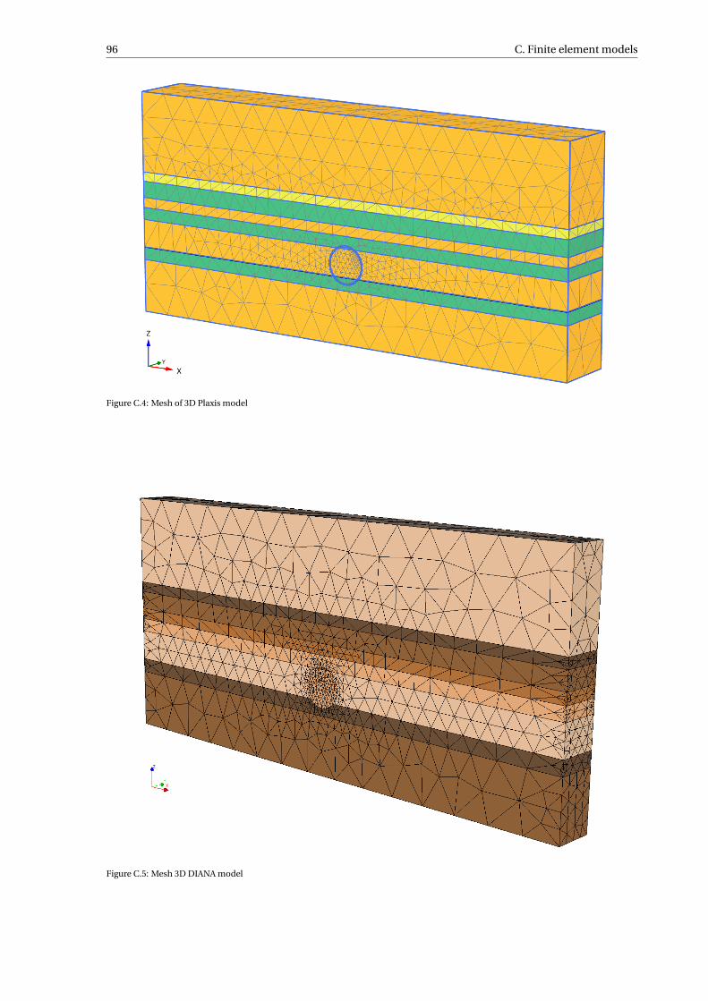
96 C. Finite element models
Figure C.4: Mesh of 3D Plaxis model
Figure C.5: Mesh 3D DIANA model

C.2. Input 97
Figure C.6: Supports of 3D Plaxis model
Figure C.7: Supports of 3D DIANA model


DAnalytical validation
Möller and Vermeer [66]N = N1 +N2 (D.1)
N1 = γH1+K0
2
R
1+ 11+νβ+ β
α
(D.2)
N2 =γH 1−K0
2 R(1+ 112(1+ν)α+ 1
4(1+ν)β)
1+ 3−2ν12(3−4ν)(1+ν)α+ 5−6ν
4(3−4ν)(1+ν)β+ 112(3−4ν)(1+ν)2 αβ
(D.3)
M =γH 1−K0
2 R2(1+ 12(1+ν)β)
2+ 3−2ν6(3−4ν)(1+ν)α+ 5−6ν
4(3−4ν)(1+ν)β+ 16(3−4ν)(1+ν)2 αβ
(D.4)
with:N Maximum Normal ForceM Maximum Bending Momentγ Unit weight of soilH Depth of tunnel axisK0 Coefficient of lateral Earth PressureR Radius of "hartlijn" tunnelν Poisson ratio of soilα,β Coefficients given by eqs. (D.5) and (D.6)
α= ER3
(E I )l(D.5)
β= ER
(E A)l(D.6)
with:E Young’s modulus of soil(E I )l Flexural rigidity of lining(E A)l Normal stiffness of lining
α= 38750 ·4.3753
1.25e +05= 25.828 (D.7)
β= 38570 ·4.375
1.225e +07= 1.378e−02 (D.8)
99

100 D. Analytical validation
value unit
Unit weight of soil 19.5 kN/m3
Depth of tunnel axis 35.4 m
Coefficient of lateral earth pressure 0.4598 -
Radius of "hartlijn" tunnel 4.375 m
Poisson ratio of soil 0.3 -
Young’s modulus of soil 38570 kN/m2
Flexural rigidity of lining 1.25e+05 kN m2/mP
rop
erti
esAxial stiffness of lining 1.225e+07 kN/m
N1 = 19.5 ·35.41+0.4598
2
4.375
1+ 11+0.3 1.378e−02 + 1.378e−02
25.828
= 2180.08kN /m (D.9)
N2 =19.5 ·35.4 · 1−0.4598
2 · (1+ 112(1+0.3) ·25.828+ 1
4(1+0.3) ·1.378e−02)
1+ 3−2·0.312(3−4·0.3)(1+0.3) 25.828+ 5−6·0.3
4(3−4·0.3)(1+0.3) 1.378e−02 + 112(3−4·0.3)(1+0.3)2 25.828 ·1.378e−02
= 673.01kN /m
(D.10)
N = 2180.08+673.01 = 2853.09kN /m (D.11)
M =19.5 ·35.4 1−0.4598
2 4.3752(1+ 12(1+0.3) 1.378e−02)
2+ 3−2·0.36(3−4·0.3)(1+0.3) 25.828+ 5−6·0.3
4(3−4·0.3)(1+0.3) 1.378e−02 + 16(3−4·0.3)(1+0.3)2 25.828 ·1.378e−02
= 557.16kN m/m
(D.12)
COB-L500 [18]N = n0(σv +σh)R +n2(σv −σh)R (D.13)
M = m2(σv −σh)R2 (D.14)
with:N Maximum Normal ForceM Maximum Bending Momentσv Total vertical stressσh Total horizontal stress (=σv ·K0)R Radius of "hartlijn" tunneln0,n2,m2 Coefficients given in eqs. (D.15) to (D.17)
1
n0= 2+ (1+K0)
2(1−ν)
(1−2ν)(1+ν)β (D.15)
1
n2= 2+ 4να
(3−4ν)(12(1+ν)+α)(D.16)
1
m2= 4+ 3−2ν
3(1+ν)(3−4ν)α (D.17)
with:K0 Coefficient of lateral earth pressureν Poisson ratio of soil

101
α,β Coefficients given in eqs. (D.15) to (D.17)
α= 12Eg R3
Ebd 3 (D.18)
β= Eg R
Ebd(D.19)
with:Eg Young’s modulus of soilEb Young’s modulus of concreted Thickness of lining
value unit
Total vertical stress 690.3 kN/m
Total horizontal stress 317.4 kN/m
Radius of "hartlijn"tunnel 4.375 m
Coefficient of lateral earth pressure 0.4598 -
Poisson ratio of soil 0.3 -
Young’s modulus of soil 38570 kN/m2
Young’s modulus of concrete 3.5e+07 kN/m2
Pro
per
ties
Thickness of lining 0.35 m
α= 12 ·38570 ·4.3753
3.5e+07 ·0.353 = 25.828 (D.20)
β= 38570 ·4.375
3.5e+07 ·0.35= 1.378e−0.2 (D.21)
1
n0= 2+ (1+0.4598)
2(1−0.3)
(1−2 ·0.3)(1+0.3)1.378e−0.2
n0 = 0.495(D.22)
1
n2= 2+ 4 ·0.3 ·25.828
(3−4 ·0.3)(12(1+0.3)+25.828)
n2 = 0.414(D.23)
1
m2= 4+ 3−2 ·0.3
3(1+0.3)(3−4 ·0.3)25.828
m2 = 0.0779(D.24)
N = 0.495 · (690.3+317.4) ·4.375+0.414 · (690.3−317.4) ·4.375 = 2857.85kN /m (D.25)
M = 0.0779 · (690.3−317.4) ·4.3752 = 556.31kN m/m (D.26)


EInterface sensitivity graphs
0°
30°
60°
90°
120°
150°
180°
210°
240°
270°
300°
330°
-3000 kN/m
-2500
-2000
-1500
Normal force for different values of Rinter
in Plaxis
Rinter
= 0.01
Rinter
= 0.05
Rinter
= 0.1
Rinter
= 0.2
Rinter
= 0.3
Rinter
= 0.5
Rinter
= 1.0
(a) Normal forces
0°
30°
60°
90°
120°
150°
180°
210°
240°
270°
300°
330°
-1000 kN m/m
-500
0
500
1000
Bending moment for different values of Rinter
in Plaxis
Rinter
= 0.01
Rinter
= 0.05
Rinter
= 0.1
Rinter
= 0.2
Rinter
= 0.3
Rinter
= 0.5
Rinter
= 1.0
(b) Bending moments
Rinter Max Min
[-] [kN/m] [kN/m]
0.01 -1901 -2482
0.05 -1896 -2421
0.1 -1846 -2413
0.2 -1759 -2489
0.3 -1678 -2579
0.5 -1546 -2723
1.0 -1457 -2791
(c) Extreme values for normal force
Rinter Max Min
[-] [kN m/m] [kN m/m]
0.01 1190 -1170
0.05 866.9 -852.3
0.1 720.1 -721.2
0.2 661.9 -655.2
0.3 639.6 -626.2
0.5 614.9 -589.9
1.0 603.3 -571.7
(d) Extreme values for bending moment
Figure E.1: Internal lining force results regarding the influence of the interface in Plaxis
103

104 E. Interface sensitivity graphs
0°
30°
60°
90°
120°
150°
180°
210°
240°
270°
300°
330°
-3000 kN/m
-2750
-2500
-2250
-2000
-1750
-1500
Normal force for different values of A in DIANA
A = 0.01
A = 0.05
A = 0.1
A = 0.2
A = 0.3
A = 0.4
A = 0.5
A = 0.6
A = 0.7
A = 0.8
A = 0.9
A = 1.0
(a) Normal forces
0°
30°
60°
90°
120°
150°
180°
210°
240°
270°
300°
330°
-750 kN m/m
-500
-250
0
250
500
750
Bending moment for different values of A in DIANA
A = 0.01
A = 0.05
A = 0.1
A = 0.2
A = 0.3
A = 0.4
A = 0.5
A = 0.6
A = 0.7
A = 0.8
A = 0.9
A = 1.0
(b) Bending moments
A Max Min
[-] [kN/m] [kN/m]
0.01 -2015 -2502
0.05 -1969 -2555
0.1 -1887 -2581
0.2 -1726 -2631
0.3 -1479 -2812
0.4 -1451 -2804
0.5 -1491 -2774
0.6 -1448 -2806
0.7 -1448 -2806
0.8 -1447 -2807
0.9 -1447 -2807
1.0 -1447 -2807
(c) Extreme values for normal force
A Max Min
[-] [kN m/m] [kN m/m]
0.01 789.5 -793.9
0.05 726.8 -716.0
0.1 711.2 -696.1
0.2 675.5 -658.7
0.3 632.5 -592.0
0.4 625.3 -583.7
0.5 626.4 -591.6
0.6 625.1 -583.1
0.7 625.1 -583.0
0.8 625.0 -582.9
0.9 625.0 -582.9
1.0 625.0 -582.8
(d) Extreme values for bending moment
Figure E.2: Internal lining force results regarding the influence of the interface in DIANA

105
0°
30°
60°
90°
120°
150°
180°
210°
240°
270°
300°
330°
-3000 kN/m
-2750
-2500
-2250
-2000
-1750
-1500
Normal force for different values of A in DIANA
A = 0.01
A(f10) = 0.01
A = 0.1
A(f10) = 0.1
A = 0.2
A(f10) = 0.2
A = 0.3
A(f10) = 0.3
A = 0.5
A(f10) = 0.5
A = 0.6
A(f10) = 0.6
A = 0.8
A(f10) = 0.8
A = 1.0
A(f10) = 1.0
(a) Normal forces
0°
30°
60°
90°
120°
150°
180°
210°
240°
270°
300°
330°
-1250 kN m/m-1000-750-500-250
0250500750
1000
Bending moment for different values of A in DIANA
A = 0.01
A(f10) = 0.01
A = 0.1
A(f10) = 0.1
A = 0.2
A(f10) = 0.2
A = 0.3
A(f10) = 0.3
A = 0.5
A(f10) = 0.5
A = 0.6
A(f10) = 0.6
A = 0.8
A(f10) = 0.8
A = 1.0
A(f10) = 1.0
(b) Bending moments
A Max Min
[-] [kN/m] [kN/m]
0.01 -2015 -2502
0.1 -1887 -2581
0.2 -1726 -2631
0.3 -1479 -2812
0.5 -1491 -2774
0.6 -1448 -2806
0.8 -1447 -2807
1.0 -1447 -2807
(c) Extreme values for normal force for f=100
A Max Min
[-] [kN m/m] [kN m/m]
0.01 789.5 -793.9
0.1 711.2 -696.1
0.2 675.5 -658.7
0.3 632.5 -592.0
0.5 626.4 -591.6
0.6 625.1 -583.1
0.8 625.0 -582.9
1.0 625.0 -582.8
(d) Extreme values for bending moment for f=100
A Max Min
[-] [kN/m] [kN/m]
0.01 -2077 -2954
0.1 -1880 -2570
0.2 -1724 -2628
0.3 -1479 -2811
0.5 -1449 -2806
0.6 -1448 -2806
0.8 -1447 -2807
1.0 -1448 -2807
(e) Extreme values for normal force for f=10
A Max Min
[-] [kN m/m] [kN m/m]
0.01 1254 -1239
0.1 716.7 -704.4
0.2 677.5 -661.5
0.3 634.0 -594.2
0.5 625.8 -584.2
0.6 625.6 -583.7
0.8 625.3 -583.3
1.0 625.1 -583.0
(f) Extreme values for bending moment for f=10
Figure E.3: Internal lining force results regarding the influence of multiplication factor for the interface strength in DIANA

106 E. Interface sensitivity graphs
0°
30°
60°
90°
120°
150°
180°
210°
240°
270°
300°
330°
-3000 kN/m
-2750
-2500
-2250
-2000
-1750
-1500
Normal force for comparison of interfaces
in Plaxis and DIANA
Plaxis 0.01
DIANA 0.01
Plaxis 0.1
DIANA 0.1
Plaxis 0.3
DIANA 0.3
Plaxis 0.5
DIANA 0.5
Plaxis 1
DIANA 1
(a) Normal forces
0°
30°
60°
90°
120°
150°
180°
210°
240°
270°
300°
330° -1250 kN m/m
-1000-750-500-250
0250500750
10001250
Bending moment comparison of interfaces
in Plaxis and DIANA
Plaxis 0.01
DIANA 0.01
Plaxis 0.1
DIANA 0.1
Plaxis 0.3
DIANA 0.3
Plaxis 0.5
DIANA 0.5
Plaxis 1
DIANA 1
(b) Bending moments
Rinter Max Min
[-] [kN/m] [kN/m]
0.01 -1900 -2482
0.1 -1842 -2418
0.3 -1674 -2583
0.5 -1542 -2728
1.0 -1454 -2794
(c) Extreme values for normal force in Plaxis
Rinter Max Min
[-] [kN m/m] [kN m/m]
0.01 1194 1174
0.1 741.0 -741.6
0.3 658.2 -645.9
0.5 632.7 -608.8
1.0 620.8 -590.2
(d) Extreme values for bending moment in Plaxis
A Max Min
[-] [kN/m] [kN/m]
0.01 -2015 -2502
0.1 -1887 -2581
0.3 -1479 -2812
0.5 -1491 -2774
1.0 -1447 -2807
(e) Extreme values for normal force in DIANA
A Max Min
[-] [kN m/m] [kN m/m]
0.01 789.5 -793.9
0.1 711.2 -696.1
0.3 632.5 -592.0
0.5 626.4 -591.6
1.0 625.0 -582.8
(f) Extreme values for bending moment in DIANA
Figure E.4: Internal lining force results regarding the influence of the interface in Plaxis and DIANA
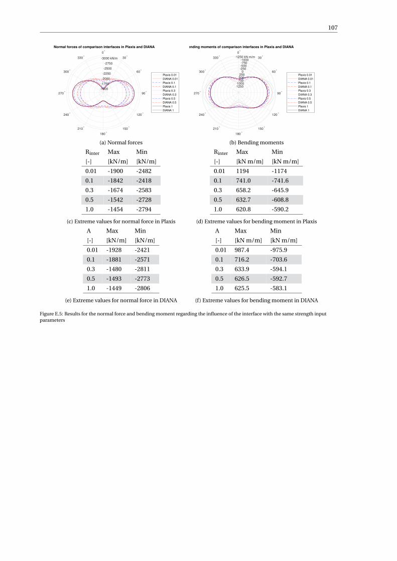
107
0°
30°
60°
90°
120°
150°
180°
210°
240°
270°
300°
330°
-3000 kN/m
-2750
-2500
-2250
-2000
-1750
-1500
Normal forces of comparison interfaces in Plaxis and DIANA
Plaxis 0.01
DIANA 0.01
Plaxis 0.1
DIANA 0.1
Plaxis 0.3
DIANA 0.3
Plaxis 0.5
DIANA 0.5
Plaxis 1
DIANA 1
(a) Normal forces
0°
30°
60°
90°
120°
150°
180°
210°
240°
270°
300°
330° -1250 kN m/m
-1000-750-500-250
0250500750
10001250
Bending moments of comparison interfaces in Plaxis and DIANA
Plaxis 0.01
DIANA 0.01
Plaxis 0.1
DIANA 0.1
Plaxis 0.3
DIANA 0.3
Plaxis 0.5
DIANA 0.5
Plaxis 1
DIANA 1
(b) Bending moments
Rinter Max Min
[-] [kN/m] [kN/m]
0.01 -1900 -2482
0.1 -1842 -2418
0.3 -1674 -2583
0.5 -1542 -2728
1.0 -1454 -2794
(c) Extreme values for normal force in Plaxis
Rinter Max Min
[-] [kN m/m] [kN m/m]
0.01 1194 -1174
0.1 741.0 -741.6
0.3 658.2 -645.9
0.5 632.7 -608.8
1.0 620.8 -590.2
(d) Extreme values for bending moment in Plaxis
A Max Min
[-] [kN/m] [kN/m]
0.01 -1928 -2421
0.1 -1881 -2571
0.3 -1480 -2811
0.5 -1493 -2773
1.0 -1449 -2806
(e) Extreme values for normal force in DIANA
A Max Min
[-] [kN m/m] [kN m/m]
0.01 987.4 -975.9
0.1 716.2 -703.6
0.3 633.9 -594.1
0.5 626.5 -592.7
1.0 625.5 -583.1
(f) Extreme values for bending moment in DIANA
Figure E.5: Results for the normal force and bending moment regarding the influence of the interface with the same strength inputparameters


FTotal displacements around tunnel
Model Three
(a) Plaxis (b) DIANA
Figure F.1: Total displacements for model three in Plaxis and DIANA
Model Four
(a) Plaxis (b) DIANA
Figure F.2: Total displacements for model four in Plaxis and DIANA
109

110 F. Total displacements around tunnel
Model Five
(a) Plaxis (b) DIANA
Figure F.3: Total displacements for model five in Plaxis and DIANA
Model Six
(a) Plaxis (b) DIANA
Figure F.4: Total displacements for model six in Plaxis and DIANA
Model Seven
Figure F.5: Total displacements for model seven in Plaxis

111
Model Nine
Figure F.6: Total displacements for model nine in Plaxis
3D model without construction phases
(a) Plaxis (b) DIANA
Figure F.7: Total displacements for front of 3D model without construction phases
(a) Plaxis (b) DIANA
Figure F.8: Total displacements of 3D model without construction phases


GHardened grout stiffness sensitivity
113

114 G. Hardened grout stiffness sensitivity
0°
30°
60°
90°
120°
150°
180°
210°
240°
270°
300°
330°
-3000 kN/m
-2500
-2000
-1500
-1000
-500
0
500
Normal force for different stiffness values
of hardened grout in DIANA
E = 25e+06
E = 10e+06
E = 1e+06
E = 500e+03
E = 400e+03
E = 300e+03
E = 200e+03
E = 100e+03
E = 80e+03
E = 60e+03
E = 40e+03
(a) Normal forces
0°
30°
60°
90°
120°
150°
180°
210°
240°
270°
300°
330°
-300 kN m/m
-200
-100
0
100
200
300
400
Bending moment for different stiffness values
of hardened grout in DIANA
E = 25e+06
E = 10e+06
E = 1e+06
E = 500e+03
E = 400e+03
E = 300e+03
E = 200e+03
E = 100e+03
E = 80e+03
E = 60e+03
E = 40e+03
(b) Bending moments
E Max Min
[kN/m2] [kN/m] [kN/m]
25e+06 590.3 -3222
10e+06 -317.6 -3156
1e+06 –1358 -2958
500e+03 -1439 -2927
400e+03 -1457 -2917
300e+03 -1475 -2901
200e+03 -1495 -2875
100e+03 -1522 -2806
80e+03 -1529 -2775
60e+03 -1537 -2727
40e+03 -1544 -2642
(c) Extreme values for normal force
E Max Min
[kN/m2] [kN m/m] [kN m/m]
25e+06 262.3 -244.3
10e+06 296.8 -268.9
1e+06 334.8 -293.7
500e+03 338.9 -298.6
400e+03 340.1 -300.5
300e+03 341.8 -303.5
200e+03 344.5 -309.1
100e+03 351.2 -323.3
80e+03 354.2 -329.6
60e+03 358.9 -339.0
40e+03 367.1 -354.6
(d) Extreme values for bending moment
Figure G.1: Results for the normal force and bending moment for different hardened grout stiffnesses in DIANA

115
0°
30°
60°
90°
120°
150°
180°
210°
240°
270°
300°
330°
-3500 kN/m
-3000
-2500
-2000
-1500
-1000
-500
0
500
1000
Normal force for different stiffness values
of hardened grout in Plaxis
E = 25e+06
E = 10e+06
E = 1e+06
E = 500e+03
E = 400e+03
E = 300e+03
E = 200e+03
E = 100e+03
E = 80e+03
E = 60e+03
E = 40e+03
(a) Normal forces
0°
30°
60°
90°
120°
150°
180°
210°
240°
270°
300°
330°
-400 kN m/m
-300
-200
-100
0
100
200
300
400
Bending moments for different stiffness values
of hardened grout in Plaxis
E = 25e+06
E = 10e+06
E = 1e+06
E = 500e+03
E = 400e+03
E = 300e+03
E = 200e+03
E = 100e+03
E = 80e+03
E = 60e+03
E = 40e+03
(b) Bending moments
E Max Min
[kN/m2] [kN/m] [kN/m]
25e+06 798.8 -3402
10e+06 -203.3 -3242
1e+06 -1372 -2925
500e+03 -1461 -2888
400e+03 -1491 -2876
300e+03 -1498 -2862
200e+03 -1515 -2835
100e+03 -1529 -2773
80e+03 -1530 -2744
60e+03 -1530 -2699
40e+03 -1524 -2616
(c) Extreme values for normal force
E Max Min
[kN/m2] [kN m/m] [kN m/m]
25e+06 324.3 -298.5
10e+06 370.7 -330.3
1e+06 419.9 -360.9
500e+03 424.6 -360.9
400e+03 425.8 -367.5
300e+03 427.4 -370.5
200e+03 429.3 -375.6
100e+03 431.9 -388.6
80e+03 433.8 -395.2
60e+03 436.6 -405.6
40e+03 441.7 -423.5
(d) Extreme values for bending moment
Figure G.2: Results for the normal force and bending moment for different hardened grout stiffnesses in Plaxis


HMN-kappa diagrams 2D
MN-κ diagrams are created to calculate deformations in concrete beams. κ is the curvature of the beam andis directly related to the stiffness of the beam through:
κ= M
E I(H.1)
EI is not a constant since it is influenced by cracking and plastic behaviour. Therefore κ is used to assess thedeformations.
The most important features of the MN-κ diagrams will be discussed briefly. Based on the internal liningforces and the properties of the lining and the reinforcement, points for the graph are determined. Walraven[80] provides the explanation and equations for the calculation of these points:
• Mr: For the moment given at this point, cracks start to form in the concrete of the lining. This point hasbeen assessed for un-reinforced concrete;
• Mb;pl: At this point, the concrete starts to behave plastically and irreversible deformations are occur-ing;
• Ms;pl: At this point, steel becomes in the plastic zone and irreversible deformations start occuring;• Current state: The current state of the internal lining forces (red point);
From the last point onwards, either Mb;pl or Ms;pl, the curvatures in the lining are plastic until the failurepoint is reached. The plastic behaviour is already considered undesirable and therefore the failure point isnot plotted. In reality, the internal lining forces start changing when cracking starts to occur. Therefore failureof the lining cannot be assessed with this approach.
In order to acquire the three points, a reinforcement has to be estimated. This reinforcement is estimatedfor model four. In order to assess which reinforcement is suitable, a unity check is done. This unity checkis the ratio between the acting moment in the lining and the moment capacity of the lining. This momentcapacity is calculated from the lining properties, normal force and reinforcement properties. A ratio below1.0 is required since it means the bending moment capacity of the lining is higher than the acting bendingmoment. A ratio above 1.0 means failure of the reinforcement. The reinforcement properties in the lining arechanged until an unity check of 0.9 is acquired.
This reinforcement is not changed throughout the different models. The purpose of this part of the re-search is to see what the influence of these construction phases is. Therefore, the amount of reinforcement iskept equal for all models.
The lowest normal force and the bending moment at the same location in servicability limit state aretaken for determination of these relations. In reality, the reinforcement is determined based on the ultimatelimit state instead of the serviceability limit state. Again, the purpose is not to acquire the right reinforcementbut to assess the influence of the different construction phases and therefore serviceability limit state will suf-fice. In reality, the lowest normal force and the matching bending moment might not be the normative liningforces. Therefore in reality, many points along the lining are assessed to calculate the reinforcement. As men-tioned earlier, the influence of the construction phases is being assessed, not the reinforcement. Thereforethe current approach is sufficient.
117

118 H. MN-kappa diagrams 2D
H.1. PlaxisModel One
Figure H.1: MN-kappa diagram Model One in Plaxis
Model Two
Figure H.2: MN-kappa diagram Model Two in Plaxis

H.1. Plaxis 119
Model Three
Figure H.3: MN-kappa diagram Model Three in Plaxis
Model Four
Figure H.4: MN-kappa diagram Model Four in Plaxis

120 H. MN-kappa diagrams 2D
Model Five
Figure H.5: MN-kappa diagram Model Five in Plaxis
Model Six
Figure H.6: MN-kappa diagram Model Six in Plaxis

H.1. Plaxis 121
Model Seven
Figure H.7: MN-kappa diagram Model Seven in Plaxis
Model Eight
Figure H.8: MN-kappa diagram Model Eight in Plaxis
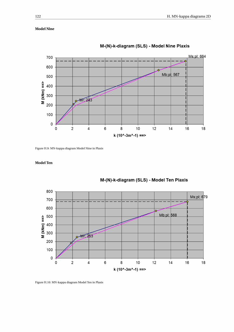
122 H. MN-kappa diagrams 2D
Model Nine
Figure H.9: MN-kappa diagram Model Nine in Plaxis
Model Ten
Figure H.10: MN-kappa diagram Model Ten in Plaxis

H.2. DIANA 123
Model Eleven
Figure H.11: MN-kappa diagram Model Eleven in Plaxis
Model Twelve
Figure H.12: MN-kappa diagram Model Twelve in Plaxis
H.2. DIANA

124 H. MN-kappa diagrams 2D
Model One
Figure H.13: MN-kappa diagram Model One in DIANA
Model Two
Figure H.14: MN-kappa diagram Model Two in DIANA

H.2. DIANA 125
Model Three
Figure H.15: MN-kappa diagram Model Three in DIANA
Model Four
Figure H.16: MN-kappa diagram Model Four in DIANA

126 H. MN-kappa diagrams 2D
Model Five
Figure H.17: MN-kappa diagram Model Five in DIANA
Model Six
Figure H.18: MN-kappa diagram Model Six in DIANA

IOne-ring models comparison
0°
30°
60°
90°
120°
150°
180°
210°
240°
270°
300°
330°
-3000 kN/m
-2500
-2000
-1500
Comparison normal force Model One
3D
2D
(a) Normal forces
0°
30°
60°
90°
120°
150°
180°
210°
240°
270°
300°
330°
-500 kN m/m
-250
0
250
500
Comparison bending moment Model One
3D
2D
(b) Bending moments
Figure I.1: Results for the normal force and bending moment for model one in 2D and 3D
0°
30°
60°
90°
120°
150°
180°
210°
240°
270°
300°
330°
-3000 kN/m
-2500
-2000
-1500
Comparison normal force Model Two
3D
2D
(a) Normal forces
0°
30°
60°
90°
120°
150°
180°
210°
240°
270°
300°
330°
-500 kN m/m
-250
0
250
500
Comparison bending moment Model Two
3D
2D
(b) Bending moments
Figure I.2: Results for the normal force and bending moment for model two in 2D and 3D
127

128 I. One-ring models comparison
0°
30°
60°
90°
120°
150°
180°
210°
240°
270°
300°
330°
-3000 kN/m
-2500
-2000
-1500
Comparison normal force Model Three
3D
2D
(a) Normal forces
0°
30°
60°
90°
120°
150°
180°
210°
240°
270°
300°
330°
-500 kN m/m
-250
0
250
500
Comparison bending moment Model Three
3D
2D
(b) Bending moments
Figure I.3: Results for the normal force and bending moment for model three in 2D and 3D
0°
30°
60°
90°
120°
150°
180°
210°
240°
270°
300°
330°
-2500
-2000
-1500
Comparison normal force Model Four
3D
2D
(a) Normal forces
0°
30°
60°
90°
120°
150°
180°
210°
240°
270°
300°
330°
-400 kN m/m
-200
0
200
400
Comparison bending moment Model Four
3D
2D
(b) Bending moments
Figure I.4: Results for the normal force and bending moment for model four in 2D and 3D
0°
30°
60°
90°
120°
150°
180°
210°
240°
270°
300°
330°
-3000 kN/m
-2500
-2000
-1500
Comparison normal force Model Five
3D
2D
(a) Normal forces
0°
30°
60°
90°
120°
150°
180°
210°
240°
270°
300°
330°
-400 kN m/m
-200
0
200
400
Comparison bending moment Model Five
3D
2D
(b) Bending moments
Figure I.5: Results for the normal force and bending moment for model five in 2D and 3D

129
0°
30°
60°
90°
120°
150°
180°
210°
240°
270°
300°
330°
-2250 kN/m
-2000
-1750
-1500
-1250
-1000
Comparison normal force Model Six
3D
2D
(a) Normal forces
0°
30°
60°
90°
120°
150°
180°
210°
240°
270°
300°
330°
-300 kN m/m
-150
0
150
300
Comparison normal force Model Six
3D
2D
(b) Bending moments
Figure I.6: Results for the normal force and bending moment for model six in 2D and 3D
0°
30°
60°
90°
120°
150°
180°
210°
240°
270°
300°
330°
-3400 kN/m
-3200
-3000
-2800
Comparison normal force Model Seven
3D
2D
(a) Normal forces
0°
30°
60°
90°
120°
150°
180°
210°
240°
270°
300°
330°
-25 kN m/m
-20
-15
-10
-5
0
5
10
Comparison bending moment Model Seven
3D
2D
(b) Bending moments
Figure I.7: Results for the normal force and bending moment for model seven in 2D and 3D with drained analysis
0°
30°
60°
90°
120°
150°
180°
210°
240°
270°
300°
330°
-3400 kN/m
-3000
-2600
-2200
Comparison normal force Model Seven undrained
3D
2D
(a) Normal forces
0°
30°
60°
90°
120°
150°
180°
210°
240°
270°
300°
330° -200 kN m/m
-150
-100
-50
0
50
100
150
200
Comparison bending moment Model Seven undrained
3D
2D
(b) Bending moments
Figure I.8: Results for the normal force and bending moment for model seven in 2D and 3D with undrained analysis

130 I. One-ring models comparison
0°
30°
60°
90°
120°
150°
180°
210°
240°
270°
300°
330°
-3200 kN/m
-3200
-2800
-2600
-2400
-2200
Comparison normal force Model Nine
3D
2D
(a) Normal forces
0°
30°
60°
90°
120°
150°
180°
210°
240°
270°
300°
330°
-200 kN m/m
-150
-100
-50
0
50
100
150
200
Comparison bending moment Model Nine
3D
2D
(b) Bending moments
Figure I.9: Results for the normal force and bending moment for model nine
0°
30°
60°
90°
120°
150°
180°
210°
240°
270°
300°
330°
-3200 kN/m
-3200
-2800
-2600
-2400
-2200
Comparison normal force Model Ten
3D
2D
(a) Normal forces
0°
30°
60°
90°
120°
150°
180°
210°
240°
270°
300°
330°
-200 kN m/m
-200
-150
-100
-50
0
50
100
150
Comparison bending moment Model Ten
3D
2D
(b) Bending moments
Figure I.10: Results for the normal force and bending moment for model ten