modelling and start-up optimization of a coal-fired power...

Department of Automatic Control

Modelling and start-up optimization of

a coal-fired power plant

Håkan Runvik

MSc ThesisISRN LUTFD2/TFRT--5950--SEISSN 0280–5316

Department of Automatic ControlLund UniversityBox 118SE-221 00 LUNDSweden

c© 2014 by Håkan Runvik. All rights reserved.Printed in Sweden by Media-Tryck.Lund 2014

Abstract

In the German electrical market, where almost no hydro power is present, the de-mand for regulating power is rising. The main reason for this is the expansion ofsolar and wind power, which is desirable from an environmental standpoint, butalso introduces large and fast variations in production. To keep the necessary bal-ance between production and consumption, the operation of thermal power plantsis changing, both in terms of stand still time and load variations. For this reason thestart-up procedure of the Vattenfall owned German lignite power plant Jänschwaldeis investigated in this thesis.

A model is created that is complex enough to describe the behaviour of thereal plant reasonably accurately, while at the same time simple enough so that op-timization of it can be performed with the optimization platform JModelica.org. Adetailed plant developed in another thesis is used to determine parameter valuesand validate the behaviour of the optimization model during simulation. The start-up procedure is handled as an optimal control problem, with constraints on stressin order to avoid damage and maximize the life length of components. Results fordifferent optimization cases are finally calculated and compared.

Keywords: JModelica.org, Dynamic optimization, Modelica, Control, Modelling,Thermal power plants

3

Acknowledgements

My biggest gratitude goes to my supervisor Stéphane Velut at Modelon AB, whohave helped me in numerous ways. His guidance regarding dynamic optimizationand JModelica.org, as well as the general planning of the project have been out-standing.

I would also like to thank Jonas Funkquist and the rest of the team at VattenfallAB, who have provided much insights into how thermal power plants and theircontrol systems work.

This work was conducted within the ITEA3 project MODRIO, which has theaim to "extend state-of-the-art modelling and simulation environments based onopen standards to increase energy and transportation systems safety, dependabilityand performance throughout their lifecycle" [MODRIO].

5

Contents

List of Figures 9List of Tables 111. Introduction 12

1.1 Aim of thesis . . . . . . . . . . . . . . . . . . . . . . . . . . . . 131.2 Structure of thesis . . . . . . . . . . . . . . . . . . . . . . . . . 13

2. Background 142.1 Power plant . . . . . . . . . . . . . . . . . . . . . . . . . . . . 142.2 Theory . . . . . . . . . . . . . . . . . . . . . . . . . . . . . . . 21

3. Dynamic optimization 253.1 Differential algebraic equations . . . . . . . . . . . . . . . . . . 253.2 DAE optimization problem . . . . . . . . . . . . . . . . . . . . 253.3 Non-linear programming . . . . . . . . . . . . . . . . . . . . . 273.4 Interior point method . . . . . . . . . . . . . . . . . . . . . . . 27

4. Programs and tools 294.1 Modelica and Dymola . . . . . . . . . . . . . . . . . . . . . . . 294.2 Optimica . . . . . . . . . . . . . . . . . . . . . . . . . . . . . . 304.3 JModelica.org . . . . . . . . . . . . . . . . . . . . . . . . . . . 30

5. Modelling 335.1 Detailed model . . . . . . . . . . . . . . . . . . . . . . . . . . . 335.2 Media models . . . . . . . . . . . . . . . . . . . . . . . . . . . 335.3 Start-up optimization model . . . . . . . . . . . . . . . . . . . . 345.4 Units . . . . . . . . . . . . . . . . . . . . . . . . . . . . . . . . 375.5 Boundary conditions and model simplifications . . . . . . . . . . 375.6 Calibration . . . . . . . . . . . . . . . . . . . . . . . . . . . . . 38

6. Optimization 416.1 Building an optimization model . . . . . . . . . . . . . . . . . . 416.2 Constraint calculation . . . . . . . . . . . . . . . . . . . . . . . 436.3 Optimization cases . . . . . . . . . . . . . . . . . . . . . . . . . 446.4 Initialization . . . . . . . . . . . . . . . . . . . . . . . . . . . . 44

7

Contents

6.5 Optimization settings . . . . . . . . . . . . . . . . . . . . . . . 457. Results 47

7.1 Phase 1 . . . . . . . . . . . . . . . . . . . . . . . . . . . . . . . 477.2 Phase 2 . . . . . . . . . . . . . . . . . . . . . . . . . . . . . . . 50

8. Discussion and Conclusions 568.1 Modelling . . . . . . . . . . . . . . . . . . . . . . . . . . . . . 568.2 Optimization . . . . . . . . . . . . . . . . . . . . . . . . . . . . 578.3 Experiences with JModelica.org . . . . . . . . . . . . . . . . . . 588.4 Conclusion . . . . . . . . . . . . . . . . . . . . . . . . . . . . . 59

Bibliography 60

8

List of Figures

2.1 Overview of a coal fired power plant. The superheaters and reheatersare denoted SH and RH, respectively, while LPP and HPP are the lowpressure and high pressure preheaters. HP-T, IP-T, and L-T are differentturbine stages. . . . . . . . . . . . . . . . . . . . . . . . . . . . . . . 14

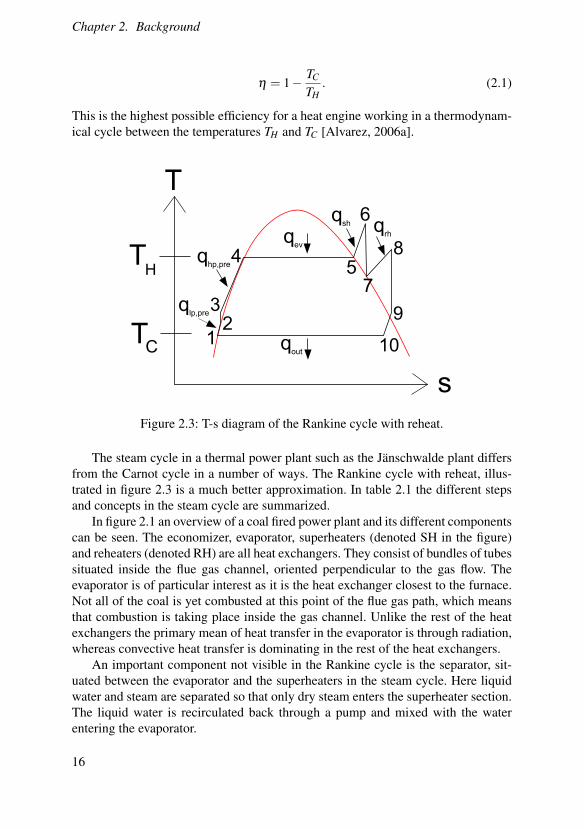
2.2 T-s (temperature vs entropy) diagram of the Carnot cycle. . . . . . . . 152.3 T-s diagram of the Rankine cycle with reheat. . . . . . . . . . . . . . 162.4 Different measured signals during a cold start-up of a block at the Jän-

schwalde power plant. Each block has two boilers which are startedseparately, named 1 and 2 in the legends. On top the coal feeder speedis illustrated, below is the water and steam flow, and the bottom plotshows the steam temperature at different points in the steam cycle. . . 19

2.5 The top plot shows the turbine speed. The electric power output is plot-ted in the middle, together with setpoints and the load schedule, whichis a reference signal for the production of the plant. Different valve po-sitions are displayed in the bottom plot. Maximum load is reached after18 hours. . . . . . . . . . . . . . . . . . . . . . . . . . . . . . . . . 20

2.6 Typical header design. . . . . . . . . . . . . . . . . . . . . . . . . . 222.7 Life time calculation using the Wöhler-curve. . . . . . . . . . . . . . 242.8 Maximal stress amplitude giving minimum stress constraint. . . . . . 24

3.1 An element with two collocation points q1 and q2. . . . . . . . . . . . 27

4.1 IPOPT output . . . . . . . . . . . . . . . . . . . . . . . . . . . . . . 32

5.1 Overview of the detailed plant model in Dymola. . . . . . . . . . . . 345.2 The optimization plant model. . . . . . . . . . . . . . . . . . . . . . 355.3 Gas and steam output temperatures for superheater 1. The input gas

mass flow and temperature are ramped in two separate stages. . . . . . 39

9

List of Figures

7.1 The calculated optimal trajectories for phase 1, case 1 in blue togetherwith simulation results with the optimal control signals as input ingreen. Dashed in red and purple are the active constraints and the set-points, respectively. One can note that the optimization algorithm man-ages to represent the system model well, as the difference between thecurves is small. The pressure and gas mass flow are ramped at maximalspeed. For the gas mass flow a large overshoot compared to the finalsteady state behaviour can be observed, which makes the temperaturereach its setpoint faster. . . . . . . . . . . . . . . . . . . . . . . . . . 48

7.2 The calculated optimal trajectories for phase 1, case 2 in blue and case3 in green, together with the active constraints marked with dashed redand the desired levels in dashed purple. The active stress constraintforces a reduced increase in gas mass flow compared to case 1. Forcase 3 only monotonously increasing gas mass flow is allowed. Themost notable result for this case is that the live steam pressure doesnot remain at its desired value for the second half of the optimizationtime, while the gas mass flow is significantly higher than in case 2. Theoptimization algorithm prioritizes the faster increase in SH4 tempera-ture the higher mass flow induces over keeping the live steam pressuresetpoint. A small deviaton from the temperature setpoint can also beobserved. . . . . . . . . . . . . . . . . . . . . . . . . . . . . . . . . 49

7.3 The calculated optimal trajectories for phase 2, case 1 in blue, togetherwith constraints marked with dashed red, and the desired SH4 temper-ature in dashed purple. The gas mass flow is ramped without any over-shoot. The stress constraint is not active, yet the bypass valve is reopened. 51

7.4 The calculated optimal trajectories for phase 2, case 2 in blue, togetherwith simulation results based on the optimization results with (green)and without (pink, dashed) the bypass reopening in the SH4 tempera-ture and bypass valve plots. Constraints are marked in dashed red andthe temperature setpoint in dashed purple. . . . . . . . . . . . . . . . 52

7.5 A comparison of the calculated optimal trajectories for phase 2, case3 (blue) and 4 (green). Active constraints are marked in dashed redand the SH4 temperature setpoint is marked in dashed purple. Themonotonous valve ratio forces more mass flow control actions in case4, in order to prevent the stress constraint from being violated. . . . . 53

7.6 The calculated optimal trajectories for phase 2, case 4 in green and case5 in blue, together with constraints marked with dashed red and thedesired SH4 temperature in dashed purple. The control action is similarfor the two cases. . . . . . . . . . . . . . . . . . . . . . . . . . . . . 54

10

7.7 The calculated optimal trajectories for phase 2, case 5 in blue and case6 in green, together with constraints marked with dashed red and thedesired SH4 temperature in dashed purple. In case 6 the further relaxedgas mass flow constraint results in a slightly longer period with stressclose to the limit compared to case 5. . . . . . . . . . . . . . . . . . . 55

List of Tables

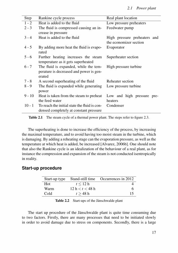
2.1 The steam cycle of a thermal power plant. The steps refer to figure 2.3. 172.2 Start-ups of the Jänschwalde plant . . . . . . . . . . . . . . . . . . . 17

5.1 Heat transfer parameter values. . . . . . . . . . . . . . . . . . . . . . 395.2 Full load heat exchanger temperature comparison. . . . . . . . . . . . 40

6.1 Critical component stress level calculations. . . . . . . . . . . . . . . 436.2 Optimization solver options . . . . . . . . . . . . . . . . . . . . . . . 45

7.1 The different optimization cases for phase 1. For the cases with reducedstress an SH4 header stress constraint of -30 MPa is used. . . . . . . . 47

7.2 Optimization convergence data for phase 1. Tcalc is the calculation timefor the solver IPOPT. . . . . . . . . . . . . . . . . . . . . . . . . . . 47

7.3 Different cost function weights give different optimization cases. Incase 5 and 6 16 elements were used, while 10 elements were used inthe rest of the cases. . . . . . . . . . . . . . . . . . . . . . . . . . . . 50

7.4 Optimization convergence data for phase 2. Tcalc is the calculation timefor the solver IPOPT. . . . . . . . . . . . . . . . . . . . . . . . . . . 50

11

1Introduction

The start-up of a thermal power plant is a complicated process with many aspects toconsider. By conducting it efficiently environmental as well as financial gains canbe achieved. The importance of the start-up schedules of thermal power plants inGermany is increasing as more wind and solar power is being installed in order toreduce the carbon dioxide emissions. To compensate for the variations in productionthe renewable sources introduce, more regulating power is needed. Hydro power isvery suitable for this purpose, but in Germany mainly thermal power is used instead.The operation of thermal power plants is therefore changing in several ways, one ofwhich is an increasing number of start-ups per year.

The start-up of the German lignite power plant Jänschwalde is examined in thisthesis. A simplified model of the plant is developed and a start-up scenario is con-sidered. New control signals are calculated by numerical solution of a dynamicaloptimization problem, with objective to reach stable working conditions. The stresson critical components is calculated and constraints are used to ensure that no com-ponents are damaged.

A first model of the Jänschwalde plant to be used for optimization was devel-oped in a previous Vattenfall-based thesis [Andersson, 2013]. The focus of thatproject was also start-up optimization and this thesis is a direct continuation of thatwork.

A highly detailed model of the Jänshwalde plant is currently developed at Vat-tenfall [Hübel et al., 2014]. To optimize this model is however impossible with thetools currently used, as it is far too complex.

Several studies of start-up optimization of combined cycle power plants havebeen conducted, such as [Casella et al., 2011] and [Lind and Sällberg, 2012]. Thelatter one is especially interesting as the methods used in that project are the sameas for the present one. In [Dietl et al., 2014] the optimization results of a developedversion of the model in [Lind and Sällberg, 2012] is presented together with otherindustrial case studies.

This thesis is conducted within the MODRIO project. MODRIO (Model DrivenPhysical Systems Operation) is a project with 38 partners in six countries. The aim

12

1.1 Aim of thesis

of the project is to improve the possibility of using modelling and simulation toolsfor system operation using open standards [MODRIO].

1.1 Aim of thesis

The starting point of this thesis is the optimization model of the Jänschwalde plantdeveloped by Eva Andersson. The description of this work can be found in [An-dersson, 2013]. The main aim of the present thesis is to greatly improve the modeland optimization results compared to that project. This aim consists of three parts.The first one is to develop a dynamic model of the plant more suitable for optimiza-tion. By doing this, the complexity and tolerances of the optimization, as well asthe formulation of the optimization problem should be improved. The second partis to make the model more similar to the real plant by adding and improving com-ponents compared to Andersson’s model. The third part is to investigate differentoptimization problem setups and find and compare optimal solutions to the start-upproblem. Another aim is to investigate how well suited the current version of theJModelica.org platform is for optimization problems such as start-up optimizationof a thermal power plant.

1.2 Structure of thesis

In Chapter 2 the function of a thermal power plant is summarized. The thermody-namics of the steam cycle is presented and the equations used to create a simplifiedmodel of the plant are explained. The optimization problem is the focus in Chapter3. The conversion from a dynamical optimization problem to a non-linear program-ming problem is explained together with the algorithm used to solve this problemnumerically.

In Chapter 4 the programs and tools used in this project are described.Different aspects of the modelling of the power plant are covered in Chapter

5. A detailed model of the plant is presented, together with key components andmodelling features of the simplified optimization model.

Chapter 6 explains the different steps in developing an optimization case whichis possible to solve without numerical problems. The specific optimization formu-lations for the start-up scenario are then presented. The corresponding results canbe found in Chapter 7.

The last chapter contains analysis of the results together a discussion of sourcesof error and possible improvements.

13

2Background

In this chapter general theory of coal fired power plants is presented, includingthe steam cycle, the start-up procedure, and the control system of the plant. Theequations that are used for the modelling of the plant are also explained.

2.1 Power plant

Located close to the city of Peitz near the German border to Poland, the Vattenfallowned power plant Jänschwalde is the largest lignite power plant in Germany. Thetotal installed capacity is 3000 GW divided into six blocks [Vattenfall], containingtwo boilers each. It was built between 1976 and 1988 and has an efficiency of about36% [Saarinen et al., 2011].

HeatingdSurfaces

Turbine

Pumps/dFansTwoAPhaseATanksCoaldMills

CombustiondChamber

Eco

SH1

CoaldddMills

ForcedADraftdFan

InducedADraftdFan

Separator

CirculationPumps

LPPd1

HPAT

HPPd7

LPPd2LPPd3LPPd4

IPAT LAT

Condenser

CondensateAPump

Evaporator

SHS

MFeedwaterA

Tank

SH3

SH4

RH1A2

SH2

RH1A1

RH2

G

HPPd6

HPPd5

FedwaterAPumpsAirAPreheater

CombustionAchamber

SH4dHeader

Figure 2.1: Overview of a coal fired power plant. The superheaters and reheatersare denoted SH and RH, respectively, while LPP and HPP are the low pressure andhigh pressure preheaters. HP-T, IP-T, and L-T are different turbine stages.

14

2.1 Power plant

A coal-fired power plant converts chemical energy stored in coal to electricalenergy. This is done in several steps. By burning the coal hot flue gas is produced.The thermal energy in the gas is used to heat water into steam, which is used to spina turbine. This mechanical energy is then converted to electricity in a generator.

Steam cycle

T

s

T

TH

Ca1

2 3

4

qin

qout

c

w

Figure 2.2: T-s (temperature vs entropy) diagram of the Carnot cycle.

For the plant model in this thesis, the most important part of the plant is thesteam cycle. Therefore it will be explained in detail below.

An idealized version of the steam cycle in a thermal power plant is the Carnotcycle. This is a thermodynamic cycle, consisting of four stages, where thermalenergy is transformed into work. In figure 2.2 the Carnot cycle is illustrated in atemperature-entropy (T-s) diagram. Each point of the curve c describes the state ofthe fluid at a certain point of the cycle, with the steam flow direction being clockwisein the diagram.

Starting from state 1, the fluid is compressed without any exchange of heat withthe environment. Next the heat qin is added to the medium at the constant tempera-ture TH . By expanding the medium isentropically the temperature is then decreased.Finally the fluid is condensed at the constant temperature TC, while the heat qoutleaves the fluid.

In order to add and subtract heat of a medium without changing its temperature itis necessary to conduct the cycle in the two-phase region, meaning that the mediumis a mix of liquid and gas. The two-phase region is the area below the curve a infigure 2.2. The grey area marked w represents the amount of work done over thecycle. Based on this, the efficiency of a Carnot-process can be derived to be

15

Chapter 2. Background

η = 1− TC

TH. (2.1)

This is the highest possible efficiency for a heat engine working in a thermodynam-ical cycle between the temperatures TH and TC [Alvarez, 2006a].

T

s

T

TH

C 123

4

6

58

7

qev

qhp,pre

qsh q

rh

qout

qlp,pre 9

10

Figure 2.3: T-s diagram of the Rankine cycle with reheat.

The steam cycle in a thermal power plant such as the Jänschwalde plant differsfrom the Carnot cycle in a number of ways. The Rankine cycle with reheat, illus-trated in figure 2.3 is a much better approximation. In table 2.1 the different stepsand concepts in the steam cycle are summarized.

In figure 2.1 an overview of a coal fired power plant and its different componentscan be seen. The economizer, evaporator, superheaters (denoted SH in the figure)and reheaters (denoted RH) are all heat exchangers. They consist of bundles of tubessituated inside the flue gas channel, oriented perpendicular to the gas flow. Theevaporator is of particular interest as it is the heat exchanger closest to the furnace.Not all of the coal is yet combusted at this point of the flue gas path, which meansthat combustion is taking place inside the gas channel. Unlike the rest of the heatexchangers the primary mean of heat transfer in the evaporator is through radiation,whereas convective heat transfer is dominating in the rest of the heat exchangers.

An important component not visible in the Rankine cycle is the separator, sit-uated between the evaporator and the superheaters in the steam cycle. Here liquidwater and steam are separated so that only dry steam enters the superheater section.The liquid water is recirculated back through a pump and mixed with the waterentering the evaporator.

16

2.1 Power plant

Step Rankine cycle process Real plant location1 - 2 Heat is added to the fluid Low pressure preheaters2 - 3 The fluid is compressed causing an in-

crease in pressureFeedwater pump

3 - 4 Heat is added to the fluid High pressure preheaters andthe economizer section

4 - 5 By adding more heat the fluid is evapo-rated

Evaporator

5 - 6 Further heating increases the steamtemperature as it gets superheated

Superheater section

6 - 7 The fluid is expanded, while the tem-perature is decreased and power is gen-erated

High pressure turbine

7 - 8 A second superheating of the fluid Reheater section8 - 9 The fluid is expanded while generating

powerLow pressure turbine

9 - 10 Heat is taken from the steam to preheatthe feed water

Low and high pressure pre-heaters

10 - 1 To reach the initial state the fluid is con-densed completely at constant pressure

Condenser

Table 2.1 The steam cycle of a thermal power plant. The steps refer to figure 2.3.

The superheating is done to increase the efficiency of the process, by increasingthe maximal temperature, and to avoid having too moist steam in the turbine, whichis damaging. By adding a reheating stage can the evaporation pressure, as well as thetemperature at which heat is added, be increased [Alvarez, 2006b]. One should notethat also the Rankine cycle is an idealization of the behaviour of a real plant, as forinstance the compression and expansion of the steam is not conducted isentropicallyin reality.

Start-up procedure

Start-up type Stand-still time Occurrences in 2012Hot t ≤ 12 h 4Warm 12 h < t < 48 h 6Cold t ≥ 48 h 15

Table 2.2 Start-ups of the Jänschwalde plant

The start up procedure of the Jänschwalde plant is quite time consuming dueto two factors. Firstly, there are many processes that need to be initiated slowlyin order to avoid damage due to stress on components. Secondly, there is a large

17


inertia in the system in general. This inertia also means that the amount of timea block has been shut down greatly affects the speed of which it can be restarted.Depending on the stand-still time a start-up procedure is categorized into hot, warmor cold in accordance with table 2.2. The three phases of the start-up procedure willbe explained next.

1. Oil burners are used to start the combustion process in the furnace. Afterstarting the coal mills the fuel is gradually changed to coal and the fuel feedis then gradually increased. The pressure is ramped up by the control systemssteering different valves. The temperature of the steam as well as the compo-nents in the system is increasing until they reach desired values. During thisphase the control valves for the different turbine stages are closed while by-pass valves are open, so that the steam does not enter the turbine. This phasetypically takes around three hours for a cold start.

2. The turbine is accelerated by opening the low pressure control valve slightly.The steam is allowed to enter the low pressure turbine first and later the highpressure. The turbine speed is increased step-wise until it reaches 3000 revo-lutions per minute. At the same time the bypass valve is closed. The tempera-ture and pressure is increased further. This phase is completed in around fourhours.

3. The generator is connected to the electrical grid, while the live steam temper-ature and pressure is increased as the load reaches its desired value. Full loadoperation with both boilers running is reached after approximately 18 hours.

In figures 2.4 and 2.5 some key signals during a start-up are plotted for a cold startof block D in the plant conducted the seventh of November 2011. It should be notedthat the two boilers of the block are not started simultaneously.

Control systemThe control system of the plant consists of several controllers on different levels.Controllers on the higher levels are providing set points for the lower level con-trollers and on the bottom level actuators and valves are steered. Of significantinterest for this project is the separator level control and the live steam pressurecontrol.

The separator level is kept constant by manipulating the feed water flow enteringthe evaporator. The mass flow affects the separator level indirectly as it decides thesteam quality of the water exiting the evaporator. That value is directly coupled tothe water level.

Two live steam pressure controllers determines the position of the high pressurecontrol and bypass valves. When the flow needs to be directed through one valveor the other the reference pressures of the controllers are altered so that they do notmatch, causing one of them to close.

18

2.1 Power plant

Timea5hourW

OpM

INxEOO°E9°E7a°aBlockaD:aColdastartablock

E x S 6 8 OE Ox OS O6 O8E

xE

SE

6E

8E

OEE

FuelafeedaboileraO

Fuelafeedaboilerax

Timea5hourW

kgps

xEOO°E9°E7a°aBlockaD:aColdastartablock

E x S 6 8 OE Ox OS O6 O8E

HE

OEE

OHE

xEE

FeedaWateraFlowaO

FeedaWateraFlowaxLiveasteamaflowaO

Liveasteamaflowax

Timea5hourW

°C

xEOO°E9°E7a°aBlockaD:aColdastartablock

E H OE OHOEE

xEE

nEE

SEE

HEE

6EE

TempabeforeaECO

TempaafteraECOTempaafteramixingapoint

TempaafteraSHS

TempaafteraSHO

TempaafteraSHxTempaafteraSHn

TempaafteraSHS

Figure 2.4: Different measured signals during a cold start-up of a block at the Jän-schwalde power plant. Each block has two boilers which are started separately,named 1 and 2 in the legends. On top the coal feeder speed is illustrated, belowis the water and steam flow, and the bottom plot shows the steam temperature atdifferent points in the steam cycle.

19


TimeaShourp

LFM

IN

ygLLwg9wg7awaBlockaD:aColdastartablock

g y V H 8 Lg Ly LV LH L8g

vgg

Lggg

Lvgg

yggg

yvgg

%gggTurbineaSpeed

TimeaShourp

MW


g y V H 8 Lg Ly LV LH L8wLgg

g

Lgg

ygg

%gg

Vgg

vgg

Hgg

ElectricaPoweraOutput

ElectricaPoweraSetpointFiringaPoweraSetpoint

LoadaSchedule

SecondaryaControlaPower

TimeaShourp

5


g y V H 8 Lg Ly LV LH L8wyg

g

yg

Vg

Hg

8g

Lgg

ValveapositionaHPaturbine

ValveapositionaIPaturbine

ValveapositionaHPabypassaLValveapositionaHPabypassay

ValveapositionaIPabypassaL

ValveapositionaIPabypassay

Figure 2.5: The top plot shows the turbine speed. The electric power output is plot-ted in the middle, together with setpoints and the load schedule, which is a referencesignal for the production of the plant. Different valve positions are displayed in thebottom plot. Maximum load is reached after 18 hours.

20

2.2 Theory

2.2 Theory

In this section theory regarding the heat exchanger models and stress calculations ispresented. The heat exchangers are very important as the heat transfer from flue gasto steam is a central part of the plant model. Furthermore, several of the equationsderived for the heat exchangers are also used in other components. Finally, the stresscalculations are of great importance as the stress is a major limiting factor duringthe start-up.

Balance equationsMass, momentum, and energy balance equations are important in many of the com-ponents of the model. The most important ones are the heat exchangers, which willbe explained in detail below. The heat exchanger model consists of two volumesconnected via a wall with one uniform temperature throughout. Steam is flowinginto and out of the volume with the mass flow rates min and mout . With positive flowdefined as flow into the volume this brings the following expression for the changein steam density ρ

min + mout =Vddt

ρ. (2.2)

The enthalpies hin and hout of the steam flowing into and out of the volume are usedto calculate the energy balance in the following way:

minhin + mouthout +Qwall =Vddt(ρu). (2.3)

The energy transferred through the media is the product of the enthalpies andtheir corresponding mass flows. In addition to this there is also an amount of heatQwall,steam transferred to the wall. The difference between the three forms of energytransfer defines the change in internal energy, which is the product of density andspecific internal energy u, of the steam inside the volume. In the gas volume corre-sponding equations apply, but the internal dynamics are assumed to be neglectable.In practice this means that the derivative terms are replaced with zeroes.

Heat transferThe heat transfer through the wall depends on the temperature of the wall. Thechange in wall temperature is determined by equation 2.4, where Mwall and cp arethe mass and the heat capacity of the wall, respectively.

Mwallcpddt

Twall = Qwall,steam +Qwall,gas (2.4)

The heat transfer between the media and the the wall are calculated using Newton’slaw of cooling, which for the steam side becomes

Qwall,steam = αwall,steamAwall,steam(Tsteam−Twall) (2.5)

21


αwall,steam is the heat transfer coefficient between the steam and the wall. A corre-sponding equation is used on the flue gas side. In the optimization model both con-stant and flow dependent heat transfer coefficients are used. In the flow dependentcase the heat transfer coefficient is decided using the Dittus-Boelter equation. Thisis a relation between the dimensionless Nusselt (Nu), Reynolds (Re), and Prandtl(Pr) numbers. For turbulent flow and cooling of the fluid it reads [Sundén, 2006]

Nu =C1ReC2PrC3 , (2.6)

with C1 = 0.023, C2 = 4/5 and C3 = 0.3. The definitions of the different dimension-less numbers now brings the following relation between heat transfer coefficient andmass flow:

α = Nuλ

D= 0.023(

ρmDµ

)4/5(cpµ

λ)0.3 λ

D, (2.7)

where λ is the thermal conductivity of the fluid, D is the the hydraulic diameter ofthe channel, µ is the dynamic viscosity and cp the heat capacity of the fluid.

The flow dependent heat transfer is used on the flue gas side in all heat exchang-ers except the evaporator.

Stress calculations

Figure 2.6: Typical header design.

The walls of several components of the plant are considered critical during thestart-up schedule of the plant. Therefore we need to calculate the stress in the wallsand use constraints on these to prevent damage and shortening of the life length ofthese components. The separator and the SH4 header are two components assumedto be critical. They both consist of cylindrical pipes connected with smaller pipes(see figure 2.6). The highest stress for these components occur on the edges of theholes at the branching points. To calculate the total stress at these points both thethermal and the mechanical stress must be determined. The mechanical stress isgiven by

σip = αm pdm

2sb(2.8)

22

2.2 Theory

Here p is the steam pressure inside the component, dm is the diameter of the pipe,sb is the wall thickness and αm is given by

αm = αm0 + fuαb, (2.9)

where αm0 = 3.2 and αb = 2.0 are constants determined by the welding of thecomponent and fu is an unroundness factor which is calculated by the followingequation

fu = 1.5dmsb

1+ 1−ν

2p

Eϑ( dm

sb)3

U (2.10)

U = 0.02 is determined by the variations in diameter of the cylinder, Eϑ is themodulus of elasticity, and ν is Poisson’s ratio for the material. The thermal stress isdetermined by

σiϑ = αϑ

βLϑ Eϑ

1−ν(Tm−Ti). (2.11)

Here the form factor αϑ = 2.0, βLϑ is the heat expansion coefficient, and Tm andTi are the mean and inner temperature of the wall. The total stress is now given bysummation:

σi = σiϑ +σip (2.12)

Another critical component is the high pressure turbine safety valve, which has aspherical shape. The stress calculations for this component are identical to those forthe cylindrical components above, except for equation 2.8, which is replaced with

σip = αm pdm

4sb. (2.13)

The operation time of a power plant can be divided into load cycles. For thescenario considered in this thesis only half of a cycle is considered, the start-up.The stress amplitude of a cycle is defined as

∆σ =σmax−σmin

2. (2.14)

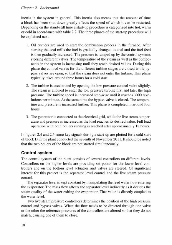
The relation between the stress amplitude ∆σ , the working temperature, and thelife length of a certain component is given by the Wöhler-curve [Meinke, 2012]. Infigure 2.7 the Wöhler-curve used for components of the Jänschwalde power plant isdisplayed for the working temperatures 100 ◦C and 550 ◦C.

It is required that the components of the power plant should withstand 4000start-ups. Together with the working temperatures, calculated as 0.75Tmax +0.25Tmin, a maximal stress amplitude can be determined for each component usingthe Wöhler-curve. This is compared with the maximal stress during a cycle foreach component to determine minimum stress constraints. The stress level reaches

23


102

103

104

105

106

102

103

104

Numberöoföcycles

2öxö

Str

essö

amp

litud

eö/öM

Pa

Wöhleröcurveö550ö°C

Wöhleröcurveö100ö°C

Figure 2.7: Life time calculation using the Wöhler-curve.

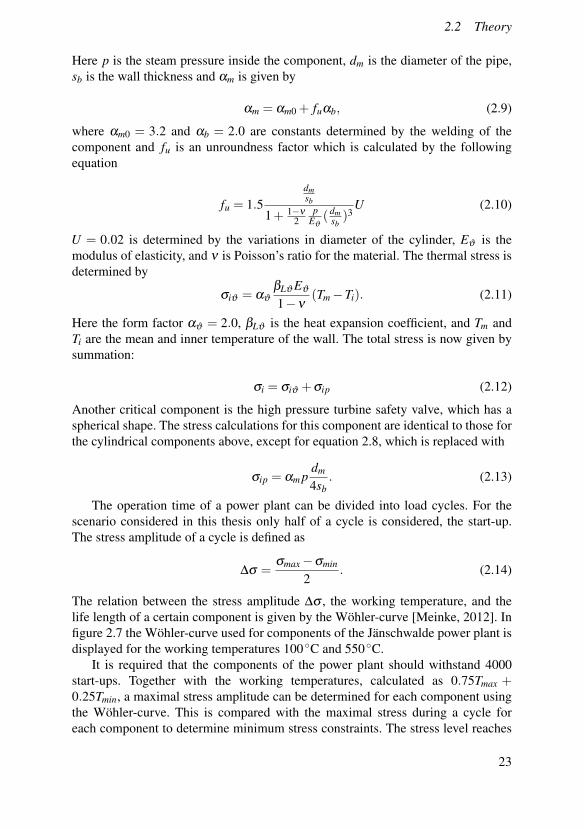
its minimal value during the start-up due to the increase in temperature that takesplace during this phase. This makes the inner temperature temporarily higher thanthe mean temperature in the walls, which according to equation 2.11 introduces anegative thermal stress component. As the increase in mechanical stress typically issmall compared to the changes in thermal stress a trough in the total stress is there-fore created. Figure 2.8 illustrates the relation between the minimal stress value, themaximal stress amplitude, and the stress constraint.

Stress

Time

2Δσ

Mechanical stressTotal stress

σmin

Figure 2.8: Maximal stress amplitude giving minimum stress constraint.

24

3Dynamic optimization

Several methods have been developed for solving dynamic optimization problems.The software used in this project uses a simultaneous approach to convert the prob-lem to a large-scale non-linear programming problem, which is solved using aninterior point method. More details about this procedure are presented below.

3.1 Differential algebraic equations

The equations which describe our plant model form a generalized system of dif-ferential equations called a differential algebraic equation (DAE) system. A DAEsystem consists of differential equations, such as equation 2.4 and algebraic equa-tions, such as equation 2.5. A general DAE system is as follows

F(x(t),x(t),u(t), t) = 0 (3.1)

where x(t) and F are vectors of variables and functions. The separation x(t) =(z(t),y(t))T , where z(t) is the differential variables and y(t) is the algebraic vari-ables is used to obtain the new formulation

F(z(t),z(t),y(t),u(t), t) = 0. (3.2)

A system of ordinary differential equations can be obtained by differentiating equa-tion 3.2. The number of differentiations needed, n, defines the differential index ofthe DAE [Ljung and Glad, 2004].

3.2 DAE optimization problem

By combining the DAE system with variable constraints and an objective function,we get a DAE optimization problem. This can be formulated in the following way,in accordance with [Biegler et al., 2001].

25

Chapter 3. Dynamic optimization

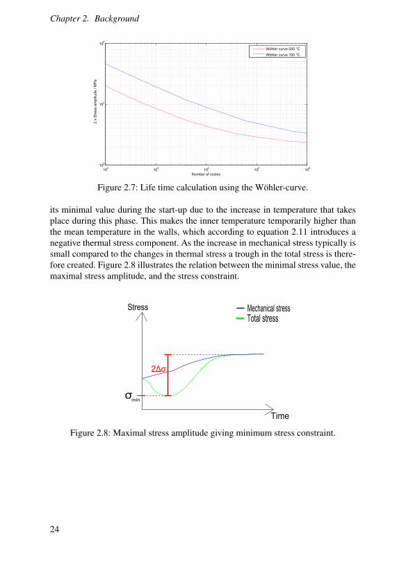
minz(t),y(t) t f ,p

ϕ(z(t f ),y(t f ),u(t f ), t f , p) (3.3a)

s.t.dz(t)

dt= F(z(t),y(t),u(t), t, p) (3.3b)

0 = G(z(t),y(t),u(t), t, p) (3.3c)

z(0) = z0 (3.3d)Hs(z(ts),y(ts),u(ts), ts, p) = 0 for s ∈ {1, . . . ,ns} (3.3e)

With the bounds:

zL ≤ z(t)≤ zU

yL ≤ y(t)≤ yU

uL ≤ u(t)≤ uU

pL ≤ p(t)≤ pU

tLf ≤ t f ≤ tU

f

where

ϕ is a scalar objective function,F are the right hand sides of differential equation constraints,

G are algebraic equation constraints, assumed to be index one,z are differential state profile vectors,

z0 are the initial values of z,y are the algebraic state profile vectors,

u are the control profile vectors,p is a time-independent parameter vector,

t f is the final time.

The objective function is typically on integral form and formulated so that devia-tions from the desired working conditions for the plant are punished. An exampleof such a function is

t f∫0

αu2 +β (T −Tre f )2dt (3.6)

where α and β are weights deciding how the objectives of keeping u close to zeroand T close to Tre f are prioritized. Alternatively a minimum time formulation canbe used. The constraints introduced in our optimization problem are inequality con-straints on control signals and stress levels.

26

3.3 Non-linear programming

3.3 Non-linear programming

t ti i+1q1 q2

Figure 3.1: An element with two collocation points q1 and q2.

To solve the DAE optimization problem numerically it is converted into a non-linear programming (NLP) problem. This is done through parameterization of stateand input profiles by Lagrange polynomials on finite elements. The elements dividethe optimization time horizon into smaller sections. For the state profiles a numberof Radau collocation points are placed inside each element. The polynomials arechosen so that they match the values and derivatives of the states at each collocationpoint, see figure 3.1. The last collocation point is placed at the end of the element.The resulting NLP can be formulated in the following way.

min f (x) (3.7a)s.t. c(x) = 0 (3.7b)

xL ≤ x≤ xU (3.7c)

3.4 Interior point method

We assume that the inequality constraints of 3.7 are on the form x ≥ 0. If they arenot this can be achieved by variable substitution and introduction of slack variables.To solve the NLP we will then introduce the following barrier problem.

min ϕµ(x) = f (x)−µ

n

∑i=1

ln(x(i)) (3.8a)

s.t. c(x) = 0 (3.8b)

27

Chapter 3. Dynamic optimization

where µ is a barrier parameter greater than zero. As the logarithmic function growstowards infinity when x goes to zero the solution to this problem will always be inthe interior of the set {x|x >= 0}. For this reason the inequality constraint can beremoved. By letting µ go to zero the solution to 3.8 will converge to the one of 3.7.For each value of µ the barrier problem is solved using the Karush-Kuhn-Tuckeroptimality conditions. These are first order necessary optimality conditions, whichfor the barrier problem according to [Biegler et al., 2001] becomes

∇ f (x)+∇c(x)y− z = 0 (3.9a)c(x) = 0 (3.9b)

XZe−µe = 0 (3.9c)x,z≤ 0, (3.9d)

where

∇ f (x) is the gradient of the objective function,∇c(x) is the gradient of the constrains,

y are the Lagrange multipliers for the equality constraints,z are the Lagrange multipliers for the bound constraints,

Z is a diagonal matrix with the elements of z,X is a diagonal matrix with the elements of x,

p is a time-independent parameter vector,e is a vector of ones.

Newton’s method is used to find a solution to this system of nonlinear equations.To verify that the found solution indeed is a minimum a method called Hessianregulation is used [Wächter, 2009].

28

4Programs and tools

The two main tools used in this project are Dymola and JModelica.org. Dymola isa commercial program for creating and simulating models written in the languageModelica, while the open cource platform JModelica.org is used for simulation andoptimization of Modelica and Optimica models.

4.1 Modelica and Dymola

The models developed within this project are written in the equation based languageModelica. It is a free standardized language where differential, algebraic, and dis-crete equations can be used to describe the models in an object-oriented way. Themain class in the language is the model class. Parameters and variables are definedin the model and in the equation section the relation between these are defined.A simple Modelica model from [JModelica.org User’s guide 2014] is displayedbelow.

model VDP

// State start values

parameter Real x1_0 = 0;

parameter Real x2_0 = 1;

// The states

Real x1(start = x1_0);

Real x2(start = x2_0);

// The control signal

input Real u;

equation

der(x1) = (1 - x2^2) * x1 - x2 + u;

der(x2) = x1;

end VDP;

Variables can have several attributes. Some of the most important ones are start,fixed, nominal, min, and max. With min and max a range for a variable can be

29

Chapter 4. Programs and tools

defined. The nominal attribute represents a nominal value used as a scaling factorto improve numerical properties. If the attribute fixed is set to true, the initialvalue of a variable is given by the start attribute. An alternative way to defineinitial values for the variables is provided by the initial equation section.

Dymola is a commercial program offering a modeling environment and a Mod-elica translator, used to transform the Modelica code into C-code which in turn isused for simulating the model. In the modeling environment models can be createdand navigated in both the text view, showing the Modelica code, and the diagramview, which is a graphical interface.

The typical way to use Dymola when creating a complex models is to arrangeand connect components in the graphical view in a way corresponding to the sys-tem one wants to represent. The connection lines represents the physical couplingbetween the components and a connector class is used to describe the equations cor-responding to the connection. The components can be found in different libraries,such as the open-source Modelica Standard library or commercial ones like theThermal power library from Modelon, but it is also possible to construct compo-nents of your own using Modelica code.

4.2 Optimica

Optimica is an extension of the Modelica language used for dynamic optimiza-tion of Modelica models. The main feature of it is the new specialized classoptimization, within which the optimization problem to be solved is defined.The attributes objective, startTime, finalTime, and static are addedto the optimization class. objective defines the type of objective function whichshould be used while startTime and finalTime define the boundaries in timefor the optimization problem. Another key element is the constraint sectionwhere equality, inequality, and point constraints can be defined . However these canalso be defined using the min and max attributes described in the previous section.For more information about Optimica, see [Åkesson et al., 2010].

4.3 JModelica.org

The open source platform JModelica.org has been used mainly for optimization, butalso simulation during the project. The optimization problem is solved by translat-ing it into a non-linear programming (NLP) problem. This is conducted by parame-terizing the state and input profiles by Lagrange polynomials [Åkesson et al., 2010]as explained in Chapter 3. The user interaction with the platform is done with thescripting language Python. Three different types of model objects can be created inJModelica.org; FMUModel, JMUModel, and CasadiModel. As the platform forusing CasadiModel was still under development during the the time the thesiswas conducted only the first two were used during this project.

30

4.3 JModelica.org

SimulationWhen simulating a model from the JModelica.org environment an FMUModel istypically used. To create such a model a functional mock-up unit (FMU), which is acompressed file following the FMI standard [FMI], is needed. The FMU is createdby compiling Modelica models, either in JModelica.org, or in some other tool thatsupport FMU export. The reason for using FMUs rather than JMUs for simulationis that the DAE of the model is converted into an ODE in the FMU, which resultsin better performance [JModelica.org User’s guide 2014]. For further informationabout the handling of FMU:s in JModelica.org see [Andersson et al., 2011]. Thepython commands used for compiling a Modelica model, loading the FMU andsimulating the resulting FMUModel are displayed below.

from pymodelica import compile_fmu

from pyfmi import load_fmu

fmu_name = compile_fmu("MyModel","MyModel.mo")

simMod = load_fmu(fmu_name)

simRes = simMod.simulate(final_time =1000)

OptimizationSimilar to the FMU, a JMU (JModelica.org model unit) is a compressed file whichcan be created through compilation of a Modelica model in JModelica.org. How-ever JMUs can also be, and usually are, created by Optimica models, as they aretypically used for optimization. By loading a JMU in JModelica.org a JMUModelis created. The following code displays how the optimization of an Optimica modelis conducted.

from pymodelica import compile_jmu

from pyfmi import JMUModel

jmu_name = compile_jmu("MyModel","MyModel.mop")

optMod = JMUModel(jmu_name)

optRes = optMod.optimize

IPOPTThe open-source software package IPOPT [IPOPT] is used to solve the non-linearprogramming problem created by JModelica.org. It uses the interior point methoddescribed in Chapter 3 and is suitable for large-scale problems. The solver producesoutput during each step of the iterative optimization procedure, a typical exampleof this can be seen in figure 4.1. Each row corresponds to one step in the iteration,while information such as step sizes, infeasibilities, and the value of the objectivefunction at each step can be found in the different columns. By interpreting thisoutput information about how to improve the optimization model can be gained.

31

Chapter 4. Programs and tools

Figure 4.1: IPOPT output

Information about the algorithms implemented in IPOPT can be found in [Wächter,2009].

32

5Modelling

The optimization model is created in Dymola. The structure of it is based on themodel created by [Andersson, 2013], but the components have been altered in sev-eral ways. Firstly, the units in all the components and the selected states in mostof them have been changed in order to make the complete model more optimiza-tion friendly. Secondly, the heat transfer model in the heat exchangers has beenimproved by the introduction of flow dependent heat transfer coefficients. There arefurthermore several new components and connections to describe the behaviour ofthe real plant better.

5.1 Detailed model

A highly complex model, attempting to describe the Jänschwalde plant and its con-trol system in a very detailed fashion, is developed in a collaboration between Vat-tenfall and Rostock University. Due to its high complexity is it not possible to usethis model for optimization purposes. It is instead used as a reference for modelstructure and parameters values. An overview of this model is displayed in figure5.1. Details about this projet can be found in [Hübel et al., 2014].

5.2 Media models

It is of great importance that the media properties of water at different pressuresand temperatures are implemented in the model with high accuracy. There are stan-dard water media models implemented in Modelica libraries for this purpose, butthese are not suitable for optimization. Therefore a library developed by ModelonAB called Water_Poly is used instead. This library contains functions to determinewater properties such as temperature. The functions are polynomial approxima-tions of standard water property functions, with enthalpy and pressure as typicalinputs. More details about this method to model water in two-phases can be foundin [Bauer, 1999]. For the flue gas no such model exists, instead constant parametersare used to model the properties.

33

Chapter 5. Modelling

Figure 5.1: Overview of the detailed plant model in Dymola.

5.3 Start-up optimization model

The optimization model of the Jänschwalde plant can be seen in figure 5.2. Manyof the key features of the steam cycle, explained in Chapter 2 are represented inthis model, as well as some thick-walled components where stress is calculated andtwo control loops. The model contains 260 equations and 40 states. The biggeststructural simplification of the optimization model is that a large part of the steamcycle is replaced with boundary conditions. The non-modelled parts include thepreheater and economizer section and the low pressure turbine. Parts that are highlysimplified are the coal mill and furnace, they are replaced with a simple gas source.

The most important components of the model are described below.

Evaporator, superheaters and reheatersThe superheaters and reheaters are together with the evaporator the most importantparts of the plant model. They are all heat exchangers with flow-dependent heattransfer coefficient on the gas side, except for the evaporator, where a constant heattransfer coefficient is used. Each heat exchanger contains three states; two describ-ing the steam, where the entire volume is lumped into one element, and one forthe wall, which also is assumed to have the same temperature throughout and isseparating the steam and the gas.

34

5.3 Start-up optimization model

Figure 5.2: The optimization plant model.

Header and high pressure safety valveThese components are modelled using a volume with a wall component attached toit. Stress on the wall is calculated using the equations described in Chapter 2. Thewalls are parametrized using three nodes in order to determine the mean tempera-ture.

Pressure drop model"Valves" are used to model the steam pressure drops that take place in the plant.They are all assumed to be linear and are situated in between other components. Forall other components (except the turbine) the steam pressure is the same at inlet andoutlet.

For the turbine bypass and pressure control loop, valves with variable conductiv-ity are used. These are used both to direct the steam flow and to control the pressurein the system.

35


TurbineIn the turbine component the steam pressure and enthalpy is decreased in accor-dance with Stodola’s law, a standard way to model steam turbines. It is a staticmodel where the mechanical power output is calculated based on the mechanicaland isentropic efficiencies.

SeparatorIn the separator the incoming water is separated into dry steam and liquid water.During normal operation two-phase water is entering the separator. The water leav-ing the blowdown at the bottom is then assumed to be saturated liquid while thewater exiting the drain is saturated steam. Balance equations are used to determinethe water level. It has a wall component with stress calculation attached to it justlike the header.

PI controllerControl loops are used in two places in the plant model; the separator level controland the live steam pressure control. The PI controller without anti-windup is chosendue to its simplicity, rather than to match the control system of the real plant exactly.For the separator level control the PI controller is implemented in a standard fashion.

For the live steam pressure control this is not possible as there are two valvesthat should determine both the live steam pressure and in which direction the steamshould flow. Therefore a solution with one controller manipulating both valves isused. An extra input is used to decide how the flowing steam is divided between thetwo routes. The following equations determine how the signal from the controlleraffects the valves.

obp =λ

100y (5.1a)

oturb =100−λ

100y (5.1b)

where y is the signal from the controller, obp and oturb are the levels of opening forthe bypass and turbine valve respectively, and λ the extra input deciding the relationbetween the valve openings. In this way each of the valves can be used for pressurecontrol, but also be closed while the other keeps the pressure.

PumpAn ideal pump model is used to create a constant flow from the blowdown of theseparator. It fixes the mass flow through it to a user defined value and the pressureof the steam is built up in the pump to correspond with this mass flow. The enthalpyis assumed to be constant.

36

5.4 Units

5.4 Units

For the optimization to work properly all important variables need to be properlyscaled. In Modelica nominal values are used for this purpose. A method that sim-plifies the effort to make sure that all variables are properly scaled is to use units,which are predefined types in the Modelica environment. Units also have the addedbenefit of an automatic check that the equations formulated in the model are physi-cally consistent. For our plant model new unit types were created. Like the units ofthe Water_Poly library these are extensions of the of the standard SI-units, but withnominal values chosen specifically to fit the conditions in our model. The methodfor deciding these values is described in Chapter 8.1.

5.5 Boundary conditions and model simplifications

As a significant part of the steam cycle is missing in the optimization plant andthe control system is highly simplified, several boundary conditions must be addedto this model. These conditions and how they have been determined are presentedbelow.

Reheat pressure boundaryIn the real plant the reheat steam pressure is decided by the low pressure turbineand bypass valves just like the high pressure turbine and bypass valves in the opti-mization plant. As the low pressure turbine system is not added in the optimizationmodel a pressure source is used instead. The profile for the pressure should ideallybe treated as optimization input, but to simplify the optimization predetermined ex-pressions were used instead. For phase 1 a linear dependency between the pressureand the steam mass flow was assumed, based on the pressure profiles of a cold startin the power plant handbook [Kraftwerk Jänschwalde 2012]. For phase 2 a constantvalue of 18 bar was used.

Flue gas enthalpyThe flue gas enthalpy was chosen so that the SH4 output temperature in the opti-mization model matched the real plant at full load. To account for the fact that thegas enthalpy is decreased for lower loads a linear dependency between gas massflow and enthalpy was assumed in accordance with equation 5.2, where the parame-ter values a=1342000 and b=1005 were chosen so to achieve a reasonable live steamtemperature for lower loads.

h = a+b · m (5.2)

Live steam pressureDuring phase 2 the live steam pressure is not used as input for the optimization,which is the case for phase 1. The reason for this is to reduce complexity of the

37


optimization problem. To obtain a ramping of the pressure during this phase a lineardependency between live steam pressure and mass flow is assumed, so that the initialand final pressure match the values from the real plant for this phase.

5.6 Calibration

Since the optimization model is highly simplified the behaviour of this plant modelwill not match the real plant exactly. However, to make the model as similar to thereal plant as possible, certain parameter values can be modified in order to minimizethe error. Ideally this task would be solved as an optimization problem, which couldbe handled by an optimization platform such as JModelica.org. A suitable techniquefor which a suitable set of free parameters and the optimal values of these wouldbe grey-box identification, details about how this method can be implemented inJModelica.org can be found in [Palmkvist, 2014]. To develop and solve such anoptimization problem is however not in the scope of this thesis. Therefore the pa-rameters are modified manually until a reasonable similarity between model andmeasurement is reached.

Heat transfer parametersThe most important experimentally determined parameter values are the heat trans-fer coefficients of the heat exchangers in the model. For each heat exchanger thesewere matched with data from the detailed plant model. However for the evaporatorthis was not possible as the evaporator of the detailed model is modelled differentlycompared to other heat exchangers. In the detailed model the main form of heattransfer is radiation, which together with recirculation of flue gas and coal combus-tion inside the component makes it very hard to compare the two models directly.Therefore the heat transfer parameters of the evaporator were chosen so that theentire system would match data from the detailed model.

ValidationFor the heat transfer parameter values of the superheaters and reheaters the valuesfrom the detailed model were used as initial guesses. Cases were created for eachheat exchanger with identical input signals (mass flow rates, pressures and so on) asthe corresponding heat exchanger in the detailed model the and the correspondingoutput signals were compared. Based on this parameter values were altered so thatthe signals matched to a reasonable degree.

For the water side mean values of the variable heat transfer coefficients in thedetailed model were used and they typically were not altered a lot. For the gas sidemean values of the different heat transfer parameters were used. The C1 parameterof equation 2.6 was then altered to reach good matching for each component. Fur-thermore, the choice C3 = 0.4 was used throughout the model, despite that this isnot the nominal value, as it seemed to get a better fit. A comparison between the

38

5.6 Calibration

Component αwall,steam / W/(m2 K) αwall,gas / W/(m2 K) C1 µ / Pa s λ / W/(m K)Evaporator 12000 195SHS 4500 0.11 5.0 ·10−5 0.092SH1 1800 0.25 3.2 ·10−5 0.053SH2 2819 0.077 3.8 ·10−5 0.065SH3 5600 0.066 4.6 ·10−5 0.084SH4 3896 0.068 4.2 ·10−5 0.072RH1A 2300 0.092 3.7 ·10−5 0.063RH1B 1800 0.105 4.0 ·10−5 0.069RH2 2200 0.074 4.4 ·10−5 0.078

Table 5.1 Heat transfer parameter values.

output of a heat exchanger from the detailed model and the optimization model canbe seen in figure 5.3, where the input gas mass flow (between 800 and 900 s) andtemperature (between 1200 and 1300 s) are ramped in separate stages. For the timespan 1000 to 1200 s the best fit can be observed, which is expected as this is theworking conditions which the chosen parameters values have been based on. In thefinal phase of the simulation there is a difference between the steam temperatures.The constant gas heat transfer properties not being accurate for this temperaturecould be a possible explanation for this.

For the evaporator the amount of transferred heat decides the water mass flow

Figure 5.3: Gas and steam output temperatures for superheater 1. The input gasmass flow and temperature are ramped in two separate stages.

39


Component Tsteam,detailed / ◦C Tsteam,opt / ◦C Tgas,detailed / ◦C Tgas,opt / ◦CEvaporator 357.8 1136.5 844.9SHS 357.9 354.9 1119.2 834.8SH1 423.3 422.8 448.2 465.4SH2 458.7 466.7 663.9 670.1SH3 504.0 501.0 972.8 812.0SH4 535.2 537.1 779.1 785.8RH1A 394.8 398.1 615.4 621.5RH1B 485.0 480.5 717.3 724.2RH2 540.0 532.5 871.1 813.4

Table 5.2 Full load heat exchanger temperature comparison.

indirectly though the separator level control. Therefore this value, together withthe gas enthalpy, was used to match the water mass flow and the superheater 4water output temperature to the corresponding values for a high load scenario of thedetailed model.

The chosen heat transfer parameter values for all heat exchangers are summa-rized in table 5.1. The steam and gas temperatures during a high load simulation ofthe detailed plant model and the optimization model are summarized in table 5.2.

For full load operation it can be noted that the steam temperatures match thedetailed plant with a precision of around 5◦C for all heat exchangers, while verylarge temperature differences can be noted on the gas side. No heat transfer throughradiation and missing heat transfer in between the modelled heat exchangers areprobably the main causes for this behaviour. The simplified modelling of the fluegas properties could also be contributing to this error. However, as the steam cycleis much more important than the behaviour of the flue gas, the mismatch in temper-atures on the gas side is acceptable.

40

6Optimization

In order to create an optimization friendly model, a large part of the total time in-vested in this project was spent investigating very simple models and optimizationcases, compared with the full plant model. The aim of this approach was to identifycomponents and parameters critical for the performance of the optimization algo-rithm and to handle the possible problems as early as possible. In the simplifiedmodels this task is much simpler than for the full plant, since the amount of param-eters and variables is much higher there. When the optimization of the simplifiedmodels worked satisfactorily, the model complexity was gradually increased withnew components. At the same time more challenging optimization cases were tried.

6.1 Building an optimization model

The first optimization case considered was to reach a certain steam temperature forone heat exchanger with the derivative of gas mass flow or temperature as input. Thenext step was to introduce a volume component with a wall with stress calculations.A constraint on the stress level was introduced in the optimization formulation. Theeffects of adding more heat exchangers and an additional volume were then in-vestigated. The number of components in the model was increased until a modeltopologically identical with the one created by [Andersson, 2013] was reached. Fi-nally, new components and connections were added to achieve a more realistic plantmodel.

Setting selectionWhile investigating simple optimization cases several optimization settings weredecided based on various tests. These choices were then used throughout the rest ofthe project. A presentation of the most important decisions can be found below.

States The formulation of the thermodynamical equations affects how suitable themodel is for optimization. For this reason a different set of states was chosen in thenew components compared to Andersson’s model. Instead of pressure and enthalpy

41

Chapter 6. Optimization

as states, density and internal energy were chosen. By doing this partial derivativeswhich in general takes on very small values were eliminated from the formulation.

By comparing the two different sets of states it can be observed that the choicedensity and internal energy leads to better performance during optimization. Thedifference is especially visible when variable scaling is not used. With pressureand enthalpy as states does scaling of the critical partial derivatives increase theconvergence speed significantly, but it is still worse than for the density and internalenergy state selection.

It can however not be said that it is always better to use density and internalenergy as states. If the water in a component mostly is in liquid phase could pressureand enthalpy be more suitable, as the in this case the changes in density are verysmall.

Scaling The choice of nominal values for variable scaling can be complicated asit is not necessarily better to scale down all variables to a magnitude around one,since the variation of the variable also needs to be considered. A better strategy isto base the scaling on the standard deviation of a variable, but this can vary betweendifferent components and optimization cases. Therefore different sets of scaling forthe different variables were tried and the setup with the best optimization conver-gence was chosen. The nominal values were in general introduced through the unitsof the variables. To cope with variables with the same unit taking different valuesextra units have been added in some instances.

Equation scaling have been necessary in two cases; in stress calculation equa-tions and equations describing the total internal energy in volumes. In both thesecases the large magnitude of the terms in the equations caused simulation problems.It has not been used otherwise.

Constraint formulation The constraints in a model are handled differently de-pending on if they are formulated as variable attributes or in the separate constraintsection, described in chapter 4.2. For the simple models no difference was observedbetween the two alternatives. However, for more complex models the optimizationperformance was clearly superior with the constraints as attributes.

A method where all min and max attributes introducing inactive constraints inthe model were removed, was tried. This idea had proven successful in anotherproject and it did affect the optimization convergence for this model too, but it didin general not improve the convergence speed.

Tolerance When optimizing models with steam pressures higher than approxi-mately 100 bar it proved necessary to increase the tolerance from the default valuein the optimization settings. The higher pressure apparently makes it harder to ob-tain solutions satisfying both optimality and the model equations with very smallerrors, which can be explained by the increased pressure makes the relative toler-ance smaller.

42

6.2 Constraint calculation

Component σmax / MPa Tmin / ◦C Tmax / ◦C ∆σ / MPa σmin / MPaSH4 header 97.5 246 537 346 -595HP safety valve 35.3 240 527 353 -671Separator 682 195 355 456 -230

Table 6.1 Critical component stress level calculations.

Convergence affecting componentsThe component causing the most difficulties during optimization was the separator.It is based on a component from the thermal power library, but altered to fit the op-timization model. The key modifications for getting the optimization to work withthe separator model included were exchanging a spline function from a hyperbolicto a polynomial function and improving the variable scaling for the water mass.The importance of scaling for the separator can be explained by the large volumeof liquid water this component contains, which makes the water mass much largerthan in other components. The liquid water also makes the selected states of den-sity and internal energy less suitable as explained in the states section above. Theintroduction of a pump connected to the blowdown might also have had a positiveresult.

It was anticipated that introducing control loops in the model would complicatethe optimization problem, as a fast start-up would require well trimmed loops. Thiswas however not observed during this project.

6.2 Constraint calculation

The constraints used in the optimization problem are very important as they defineboundaries for the operation of the plant.

Stress constraintsSimulations give the maximal stress levels for each of the critical components andtheir working temperatures. These are summarized in table 6.1, together with themaximal stress amplitudes, which are calculated with the Wöhler-curve based onthe temperatures. The corresponding minimum stress constraints can also be foundin the table, calculated in accordance with figure 2.8.

Flue gas mass flowThe speed of which the flue gas mass flow can be increased or decreased is also con-strained. To approximate how fast it is allowed to change simulation data from thedetailed plant model is used. By examining the changes in gas mass flow when theplant switches between different loads a constraint of ±0.15 kg/s2 is derived. How-ever, as this empirical value might not be the actual limit for the plant constraints of±0.26 kg/s2 and ±0.5 kg/s2 are also tried.

43


Pressure set pointIt also proved necessary for optimization purposes to constraint how fast the livesteam pressure setpoint could be changed. As it is not known how fast changes arefeasible in the real plant a value of ±0.03 bar/s was chosen.

Valve opening ratioThe constraints on the speed of valve opening ratio changes are chosen so that theyin general do not get active. The exception is cases where only monotonous ratiochanges are allowed, then the minimum constraint is set to zero.

6.3 Optimization cases

To simplify the optimization formulations the start-up scenario was split into twophases roughly corresponding to the last part of phase one and entire phase two ofthe start-up of the real plant.

Phase 1For phase 1 the temperature and pressure profiles are optimized with the live steamcontroller pressure setpoint and the gas mass flow as input. Deviations from objec-tive live steam pressure and temperature are included in the cost function as wellas the control signals. Minimum constraints are used on the wall stress of the SH4header and the separator. The turbine valve is closed during this phase and the wholeturbine section is therefore removed from the model. The initial live steam pressureand gas mass flow of the optimization scenario are chosen to be 15 bar and 26 kg/s.The desired live steam pressure and temperature are 80 bar and 618 K, respectively.

Phase 2In this phase the objectives are an increased live steam temperature and bypassvalve closing. The live steam pressure is chosen to be linearly dependent on the livesteam mass flow and is therefore also increased. A stress constraint on a safety valvein the turbine steam route is added, which prevents the bypass valve from closingimmediately. The start of the optimization scenario matches the final conditions ofphase 1, with a live steam pressure of 80 bar and a gas mass flow of 100 kg/s. Thegoal of this phase is to reach a live steam temperature of 808 K, with a correspondinglive steam pressure of 121 bar.

6.4 Initialization

In order to find a solution to the NLP problem the optimization algorithm is de-pendent on a good initialization. In this project an initial trajectory was created bysimulating the optimization model. The model was typically simulated twice, with

44

6.5 Optimization settings

Option Chosen value CommentMu strategy AdaptiveNumber of elements 10-16 Depending on optimization caseTolerance 5 ·10−6

Acceptable tolerance 3 ·10−5

Blocking factors Ones Control signal constant over each element

Table 6.2 Optimization solver options

the first results being discarded in order to avoid fast transients during the first partof the optimization. The initial values for the optimization and the initial trajectorieswere then taken from the second simulation. For phase 2 a steady state initial tra-jectory with all inputs at zero proved sufficient to obtain good convergence for theoptimization algorithm. For phase 1 constant non-zero inputs for both control sig-nals were used during initialization, bringing the system closer to the desired statefor the final time than zero inputs would do. It proved hard to achieve convergenceof the optimization without this ramping.

6.5 Optimization settings

There are many settings that need to be specified in order to achieve a good opti-mization results. These options range from solver options to specific formulations inthe actual model. Some of these are general while others need to be chosen manuallyto fit each specific optimization case. The two main goals when determining thesesettings have been to get the optimization algorithm to converge within a reasonableamount of time and to get a high result quality, which means a fine discretizationand low values on tolerances. The secondary goal is to modify the characteristics ofthe solution so that it is reasonable and that the right objectives are prioritized.

Solver optionsIn the Python environment several settings can be manipulated. These affect howthe optimization problem is solved. The changes from the default settings that wereused in this project are summarized in table 6.2. The tolerances were chosen as lowas possible while keeping convergence to a solution. The number of elements affectboth the time per iteration and the number of iterations needed to find a solution.For this value a compromise between high resolution and calculation time needs tobe made. The blocking factors are used to limit the freedom of the control signal.The notation in the table indicates that the control signals must be constant for eachelement.

45


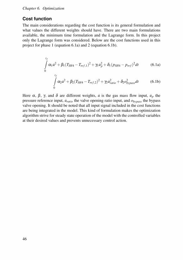
Cost functionThe main considerations regarding the cost function is its general formulation andwhat values the different weights should have. There are two main formulationsavailable, the minimum time formulation and the Lagrange form. In this projectonly the Lagrange form was considered. Below are the cost functions used in thisproject for phase 1 (equation 6.1a) and 2 (equation 6.1b).

t f∫0

α1u2 +β1(TSH4−Tre f ,1)2 + γ1u2

p +δ1(pSH4− pre f )2dt (6.1a)

t f∫0

α2u2 +β2(TSH4−Tre f ,2)2 + γ2u2

ratio +δ2o2bypassdt (6.1b)

Here α , β , γ , and δ are different weights, u is the gas mass flow input, up thepressure reference input, uratio the valve opening ratio input, and obypass the bypassvalve opening. It should be noted that all input signal included in the cost functionsare being integrated in the model. This kind of formulation makes the optimizationalgorithm strive for steady state operation of the model with the controlled variablesat their desired values and prevents unnecessary control action.

46

7Results

7.1 Phase 1

The components assumed to be critical for the first phase, the SH4 header and theseparator, proved uncritical during the start-up, as described in the section for case 1below. The most likely explanation for this result is that other components are moresensitive than the ones considered in this thesis. Therefore a stricter constraint on theSH4 header was introduced in order to illustrate how this phase of the optimizationcould be conducted. A minimum constraint of -30 MPa was used for the cases2 and 3. The optimization cases are summarized in table 7.1, while optimizationconvergence data can be found in table 7.2. The gas mass flow constraint is 0.15kg/s2 for all cases. No larger values were tried as this constraint rarely got active.Twelve elements were used in all cases, which created a NLP problem with 10592equations. For phase 1, with the more restrictive SH4 header stress constraint used,the final live steam conditions are reached in approximately 4000 seconds. One cannote that the calculation time for the solver is small compared to the start-up timeof the plant, making real time implementations possible.

Case α β γ δ Final time / s Stress reduced Monotonous gas flow1 0.0001 0.001 0.0001 0.0001 4000 No No2 0.0001 0.001 0.0001 0.0001 8000 Yes No3 0.0001 0.001 0.0001 0.0001 8000 Yes Yes

Table 7.1 The different optimization cases for phase 1. For the cases with reducedstress an SH4 header stress constraint of -30 MPa is used.

Case Iterations Tcalc / s Solution type1 51 69.4 Optimal2 48 61.7 Optimal3 39 48.6 Optimal

Table 7.2 Optimization convergence data for phase 1. Tcalc is the calculation timefor the solver IPOPT.

47

Chapter 7. Results

Case 1: stress constraint uncriticalResults for the first optimization case considered for phase 1 can be seen in figure7.1 together with simulation results with the calculated optimal input signals. Thegas mass flow and live steam pressure is ramped with maximal speed, with a largeovershoot in gas mass flow in order to reach the desired temperature fast. The min-imum stress level of -134 MPa for the SH4 header is far from the constraint andcorresponds to a stress amplitude of 116 MPa. The corresponding number of cy-cles, calculated with the Wöhler curve is 15700000. The comparison between theoptimization output and the simulation data provides an estimate of how well theoptimization algorithm manages to solve the DAE system that represents the opti-mization model. In general the signals match to a large degree, but some differencecan be observed for the SH4 header stress. The separator stress is also uncritical,with the increased temperature only giving a very small dip in stress during the first

Figure 7.1: The calculated optimal trajectories for phase 1, case 1 in blue togetherwith simulation results with the optimal control signals as input in green. Dashedin red and purple are the active constraints and the setpoints, respectively. One cannote that the optimization algorithm manages to represent the system model well,as the difference between the curves is small. The pressure and gas mass flow areramped at maximal speed. For the gas mass flow a large overshoot compared to thefinal steady state behaviour can be observed, which makes the temperature reach itssetpoint faster.

48

7.1 Phase 1

200 seconds.

Case 2: restrictive SH4 header constraintTrajectories and optimal control signals for this case, which has a more restrictiveSH4 header constraint of -30 MPa, are summarized together with case 3 in figure7.2. A large overshoot can be observed for the gas mass flow like in case 1. The gasflow is reduced to prevent the constraint from being violated, while the pressure isramped up at close to maximal speed until the desired value is reached.

Pres

sure

cont

rol s

ignal

0.02

0.01

0.00

0.01

0.02

0.03

0.04

Time / s

Time / s Time / s

Time / s

Figure 7.2: The calculated optimal trajectories for phase 1, case 2 in blue and case 3in green, together with the active constraints marked with dashed red and the desiredlevels in dashed purple. The active stress constraint forces a reduced increase in gasmass flow compared to case 1. For case 3 only monotonously increasing gas massflow is allowed. The most notable result for this case is that the live steam pressuredoes not remain at its desired value for the second half of the optimization time,while the gas mass flow is significantly higher than in case 2. The optimizationalgorithm prioritizes the faster increase in SH4 temperature the higher mass flowinduces over keeping the live steam pressure setpoint. A small deviaton from thetemperature setpoint can also be observed.

Case 3: monotonously increasing gas mass flowThe results for a case where only monotonously increasing gas mass flow is allowedcan be seen in figure 7.2. Interestingly the final conditions of the optimization re-sults are different from the desired working conditions. The live steam pressure isramped to higher value than the setpoint in order to achieve a faster increase in live

49

Chapter 7. Results

steam temperature. However, it is then decreased to a value of approximately 70bar, significantly lower than the setpoint of 80 bar. The gas mass flow is ramped toa value around 112 kg/s, which results in too high live steam temperature when thepressure is 80 bar, but gives a more correct temperature for the lower pressure. How-ever the temperature is also slightly too high. The reason for this strange result isthat the faster increase in temperature during the first part of the scenario the highermass flow results in compensates for the constant error in pressure during the lasthalf. However, this result obviously is not practically useful as the desired state forswitching to phase 2 is not reached. To avoid this problem additional constraints onpressure and temperature for the final time of the optimization can be implemented.

7.2 Phase 2

The different optimization cases for this phase are summarized in table 7.3. Threedifferent gas mass flow constraints are used, 0.15 kg/s2 , 0.26 kg/s2, and 0.5 kg/s2.Depending on the number of elements, 10 for the first four cases and 16 for case5 and 6, the number of equations in the NLP problems were 100098 and 15792,respectively. Optimization convergence data can be seen in table 7.4. The desiredlive steam conditions are reached in approximately 3000 seconds with restrictivegas flow changes and 2000 seconds otherwise. The calculated trajectories for thedifferent cases are explained in the following sections.

Case α β γ δ Final time / s Gas flow limit / kg/s2 Bypass valve reopening1 0.0006 0.002 14 0.001 7000 0.15 Yes2 0.00001 0.0005 40 0.001 7000 0.15 Yes3 0.00001 0.0005 40 0.001 4000 0.26 Yes4 0.00001 0.0005 40 0.001 4000 0.26 No5 0.00001 0.0005 40 0.001 4000 0.26 No6 0.00001 0.0005 40 0.001 4000 0.50 No

Table 7.3 Different cost function weights give different optimization cases. In case5 and 6 16 elements were used, while 10 elements were used in the rest of the cases.

Case Iterations Tcalc / s Solution type1 76 79.7 Optimal2 56 60.5 Optimal3 131 167.5 Optimal4 56 94.0 Optimal5 57 100.6 Optimal6 67 118.0 Optimal

Table 7.4 Optimization convergence data for phase 2. Tcalc is the calculation timefor the solver IPOPT.

50

7.2 Phase 2

Case 1: bypass valve reopeningIn figure 7.3 optimal control signals are visualized together with the most impor-tant model variable trajectories for case 1. The gas flow is increased with maximalcontrol action to reach the desired temperature fast. The stress constraint on the se-curity valve does not get active during this ramping, but the bypass valve is anywayreopened. The most likely reason for this unexpected behaviour is that the weight onthe bypass term in the cost function is relatively small, which makes the objectiveof bypass valve closing less important compared to the SH4 temperature objective.The cost function should still be reduced by closing the valve faster, but it is possiblethat the difference is smaller than the optimization tolerance.

Case 2: bypass valve prioritizedFor this case the weight on bypass valve opening is significantly larger comparedto case 1. The effects of this can be observed in the trajectories displayed in figure7.4. Due to the higher weight the reopening of the bypass valve is smaller in am-plitude and the initial closing is more complete. This results in a lower safety valvestress amplitude compared to case 1, as the pressure induced temperature changesare smaller when the valve is operated in a calmer fashion. To investigate if thesmall reopening of the bypass valve has any indirect affect on the SH4 temperature

7

Figure 7.3: The calculated optimal trajectories for phase 2, case 1 in blue, togetherwith constraints marked with dashed red, and the desired SH4 temperature in dashedpurple. The gas mass flow is ramped without any overshoot. The stress constraint isnot active, yet the bypass valve is reopened.

51

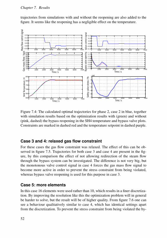
Chapter 7. Results

trajectories from simulations with and without the reopening are also added to thefigure. It seems like the reopening has a negligible effect on the temperature.

Figure 7.4: The calculated optimal trajectories for phase 2, case 2 in blue, togetherwith simulation results based on the optimization results with (green) and without(pink, dashed) the bypass reopening in the SH4 temperature and bypass valve plots.Constraints are marked in dashed red and the temperature setpoint in dashed purple.

Case 3 and 4: relaxed gas flow constraintFor these cases the gas flow constraint was relaxed. The effect of this can be ob-served in figure 7.5. Trajectories for both case 3 and case 4 are present in the fig-ure, by this comparison the effect of not allowing redirection of the steam flowthrough the bypass system can be investigated. The difference is not very big, butthe monotonous valve control signal in case 4 forces the gas mass flow signal tobecome more active in order to prevent the stress constraint from being violated,whereas bypass valve reopening is used for this purpose in case 3.

Case 5: more elementsIn this case 16 elements were used rather than 10, which results in a finer discretiza-tion. By improving the resolution like this the optimization problem will in generalbe harder to solve, but the result will be of higher quality. From figure 7.6 one cansee a behaviour qualitatively similar to case 4, which has identical settings apartfrom the discretization. To prevent the stress constraint from being violated the by-

52

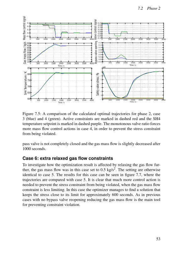
7.2 Phase 2

Figure 7.5: A comparison of the calculated optimal trajectories for phase 2, case3 (blue) and 4 (green). Active constraints are marked in dashed red and the SH4temperature setpoint is marked in dashed purple. The monotonous valve ratio forcesmore mass flow control actions in case 4, in order to prevent the stress constraintfrom being violated.

pass valve is not completely closed and the gas mass flow is slightly decreased after1000 seconds.

Case 6: extra relaxed gas flow constraintsTo investigate how the optimization result is affected by relaxing the gas flow fur-ther, the gas mass flow was in this case set to 0.5 kg/s2. The setting are otherwiseidentical to case 5. The results for this case can be seen in figure 7.7, where thetrajectories are compared with case 5. It is clear that much more control action isneeded to prevent the stress constraint from being violated, when the gas mass flowconstraint is less limiting. In this case the optimizer manages to find a solution thatkeeps the stress close to its limit for approximately 600 seconds. As in previouscases with no bypass valve reopening reducing the gas mass flow is the main toolfor preventing constraint violation.

53

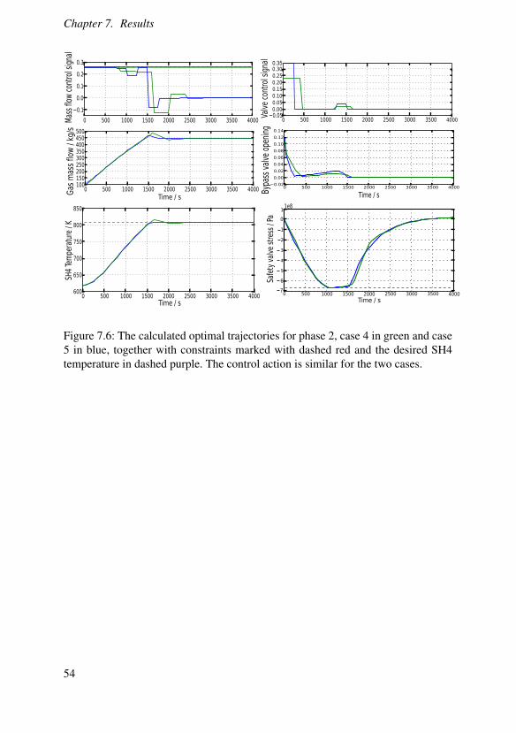
Chapter 7. Results

6

7

0.35

Figure 7.6: The calculated optimal trajectories for phase 2, case 4 in green and case5 in blue, together with constraints marked with dashed red and the desired SH4temperature in dashed purple. The control action is similar for the two cases.

54

7.2 Phase 2

6

7

0.35

Figure 7.7: The calculated optimal trajectories for phase 2, case 5 in blue and case6 in green, together with constraints marked with dashed red and the desired SH4temperature in dashed purple. In case 6 the further relaxed gas mass flow constraintresults in a slightly longer period with stress close to the limit compared to case 5.

55

8Discussion andConclusions

8.1 Modelling

The level of complexity of the optimization model is believed to capture most of therelevant behaviour of the real plant. However, as the number of matching parametersin the model is quite large, the parameter values chosen in this project are not theoptimal ones and therefore a clear difference can be observed for some variables,especially many of the gas temperatures. One could also argue that the cause forthis is that not all of the heat exchangers in the real plant have exact counterpartsin the optimization model, since the heat exchangers in the model in some casesrepresent not only the corresponding heat exchanger in the real plant, but also someheat exchange happening in between the heat exchangers.

Furthermore, the matching between the models is only verified for close to fullload. In order to get a more useful optimization model it is necessary to make surethat the behaviour of the model is also correct for lower loads.

Further workThere are two main directions for improving the optimization model so that the be-haviour gets more similar to the real plant. The first is to improve parameter values,such as heat transfer coefficients, boundary conditions and control system param-eters and setpoints. It would be desirable to decide these values in a systematicmanner with the objective of matching the real plant in the range of temperatures,pressures and mass flows that are present during the start-up. Grey-box identifica-tion could be a suitable technique for this purpose.

The second direction is to improve the components and structure of the plantmodel to improve its behaviour. There are many phenomena not accounted for in thecurrent model such as heat transfer through radiation, heat transfer in between heatexchangers, and the spray water cooling system. However, whenever new physicalphenomena are added to the model, it is important to verify that the increase in

56

8.2 Optimization

accuracy is large enough to compensate for the extra complexity in the optimization.For this reason another possible step in the modelling task would be to reduce thenumber of heat exchangers to investigate if the dynamics between input and outputfor the whole chain of heat exchangers could be described by a simpler system. Ifthe decrease in accuracy would not be too great this could be a way to simplifythe system, which would make the optimization problem less complex. However,having a model structure similar to the real plant has clear benefits apart from givingbetter accuracy, as it simplifies the choice of parameter values and improves thegeneral understandability of the model.

To develop a coal and flue gas media model suitable for optimization could alsoincrease the accuracy of the model. This would bring the extra benefit of removingat least some of the empiric parameters in the heat exchangers, as heat capacitiesand possibly other medium properties could be calculated automatically instead.Whether it is worthwhile to introduce a mill and combustion system is an interest-ing question. In the current model the change in gas mass flow is assumed to bedirectly controllable, something that is not true for the real plant. The question isif the proposed optimal mass flow schedule can be achieved by the correspondingsystem in the real plant. If this is the case it would be unnecessary to add these com-ponents as they have no other affect on the model. If it is not possible to achieve thismass flow one would need to consider adding extra components, or at least alter theconstraints on the gas mass flow to fit the behaviour of the real plant.

8.2 Optimization

Compared to the previous project regarding the Jänschwalde plant, great improve-ments have been achieved regarding the optimization despite a significantly greatermodel complexity. However, more work is needed before the control algorithmsdeveloped in this thesis could be applied to the real plant.

In this project variable scaling and state selection have both proven importantfor achieving good optimization results. Improvements in these areas are the biggestreason for the improved result quality. It is however still worth investigating the stateselection further, as density might not be optimal for components where only liquidwater is present.

By comparing different optimization cases it is clear that the optimal trajecto-ries are highly dependent on optimization settings such as cost function weights.This is desirable in the sense that it gives freedom to the user to manipulate the be-haviour of the plant during the start-up scenario, but it also means that more workis needed to decide which objectives that should be prioritized. If more constraintsare introduced into the model to account for the limitations of the real plant thisphenomenon would probably be reduced.

57

Chapter 8. Discussion and Conclusions

Possible improvementsAs there are many parameters to determine for the optimization problem, the setupchosen in this project is not the optimal. The general strategy when deciding theseparameter values has been to attempt to find good values for each parameter in-dependently. Due to the number of settings possible this is the only method onecould use within a reasonable time frame and by spending time finding better val-ues for these parameters better discretization and tolerance levels could probably beachieved.

A step that might result in a more optimal result would be to handle both thephases in the start-up as one optimization problem. The current setup, with a fixedpoint in which the optimization inputs and objectives are changed might not give anoptimal result. Firstly, the second part of the optimization is not considered duringphase one. Secondly, there might be a better switching point. However, one needs tobe careful when deciding whether to change this, as it might get harder to implementthe control in the real plant if the calculated start-up schedule is too different fromthe current scheme.

To get better optimization results one could also try using the optimization soft-ware on a system with more computational power. This would increase the speedof the optimization, which would make it possible to run optimizations with moreiterations or with more calculations (meaning finer discretization or more complexmodel) per iteration. However, during this project the computational time can notbe said to have been a too limiting factor.

The optimization problem formulation could also be improved. The objectiveof the optimization would be better defined by including terms such as generatedpower or fuel consumption in the cost function. By doing this the environment andfinancial gains from optimizing the start-up procedure would be clearer and thechoice of cost function weights would become less arbitrary. A minimum time for-mulation could also be evaluated, something that has not been tried during thisthesis.

8.3 Experiences with JModelica.org

The JModelica.org platform has proven very powerful for optimization purposesduring this thesis. Solutions to all reasonable optimization problem formulationstried in the project have eventually been found and in general the optimization soft-ware has not been a limiting factor. However, some aspects of the platform couldbe improved. Currently much time needs to be spent on issues such as scaling andin many cases the convergence of the optimization algorithm is very sensitive toparameter changes and the working conditions of the model.

If some of this work could be handled automatically by the tool and if the inter-action with the program could be simplified for the user it would be less time con-suming to investigate different optimization cases. Some suggested improvements

58

8.4 Conclusion

are therefore a better handling of variable scaling and equation scaling. To introduceshifting of variables could also be considered, as well as a general improvement ofthe user interaction, possibly with a graphical interface. Some of these issues mighthowever be resolved with the introduction of the CasADi platform.

The following specific problems with the software were encountered throughoutthe course of the project:

• Poorly scaled equations caused problems, when trying to simulate FMU mod-els with JModelica.org for certain versions of the platform.

• Certain formulations of initial equations made it impossible to simulate FMUmodels.

8.4 Conclusion

The results of this thesis show that it is possible to develop reasonably complexoptimization cases for thermal power plant start-ups using JModelica.org and Dy-mola. However, to achieve this, one needs to focus on adapting every part of themodel so that it is suitable for optimization. As JModelica.org is a platform underdevelopment some aspects of this process might be simplified in the future.

During the project it has also been observed that the matching of a simplifiedmodel to a more complex one is a difficult task to perform by hand for models ofthis complexity. Changing one parameter value typically affects the model in morethan one way, which makes it hard to decide correct values as the parameters cannot be treated independently.

A big remaining step between the function of the current optimization modeland the usage of it in the real plant is the matching of the two systems. Despite thesimilarities between the two systems there are also large differences, both in termsof the physical modelling and the control systems. In order to implement controlstrategies developed with JModelica.org more work is needed. The optimizationmodel needs to be developed further and some alterations of the control of the realplant are probably also needed. A suitable next step towards this goal would beto use an optimization model to calculate the control signals during a simulationof a start-up scenario of the detailed plant model. By doing this one would get avery good indication of how an implementation for the real plant would work. An-other possible approach would be to use optimal trajectories calculated with JMod-elica.org to develop the start-up strategy off line. This method would be simpler asit does not require any direct interaction between the systems.

59

Bibliography

Åkesson, J., K.-E. Årzén, M. Gäfvert, T. Bergdahl, and H. Tummescheit (2010).“Modeling and optimization with Optimica and JModelica.org—languages andtools for solving large-scale dynamic optimization problems”. Computers andChemical Engineering 34:11, pp. 1737–1749.

Alvarez, H. (2006a). Energiteknik del 1. Studentlitteratur, Lund.Alvarez, H. (2006b). Energiteknik del 2. Studentlitteratur, Lund.Andersson, C., J. Åkesson, C. Führer, and M. Gäfvert (2011). “Import and export

of functional mock-up units in jmodelica.org”. In: 8th International ModelicaConference. Dresden, Germany.

Andersson, E. (2013). Development of a dynamical model for start-up optimizationof coal-fired power plants. MA thesis. KTH. URL: http://www.control.lth.se/documents/1999/5629.pdf.

Bauer, O. (1999). Modelling of two-phase flows with Modelica. MA thesis. Depart-ment of Automatic Control, Lund University, Sweden. URL: http://www.control.lth.se/documents/1999/5629.pdf.

Biegler, L. T., A. M. Cervantes, and A. Wächter (2001). “Advances in simultaneousstrategies for dynamic process”. Chemical Engineering Science 57, pp. 575–593.

Casella, F, M Farina, F Righetti, R Scattolini, D Faille, F Davelaar, A Tica, HGueguen, and D Dumur (2011). “An optimization procedure of the start-up ofcombined cycle power plants”. In: 18th IFAC world congress. Milano, Italy,pp. 7043–7048.

Dietl, K, S Gallardo Yances, A Johnsson, J Åkesson, K Link, and S Velut (2014).“Industrial application of optimization with modelica and optimica using intel-ligent python scripting”. In: 10th International Modelica Conference. Lund.

FMI. https://www.fmi-standard.org/. Accessed 2014-05-06.

60

Bibliography

Hübel, M, A Berndt, S Meinke, M Richter, P Mutschler, E Hassel, H Weber, MSander, and J Funkquist (2014). “Modelling a lignite power plant in modelicato evaluate the effects of dynamic operation and offering grid services”. In: 10thInternational Modelica Conference. Lund.

IPOPT. https://projects.coin-or.org/Ipopt. Accessed 2014-05-06.JModelica.org User’s guide (2014). http://www.jmodelica.org/page/6212.

Accesed 2014-05-10.Kraftwerk Jänschwalde (2012). Plant handbook, internal document. Vattenfall.Lind, A. and E. Sällberg (2012). Optimization of the Start-up Procedure of a Com-

bined Cycle Power Plant. MA thesis. Department of Automatic Control, LundUniversity, Sweden.

Ljung, L. and T. Glad (2004). Modellbygge och simulering. Studentlitteratur, Lund.Meinke, S. (2012). Modellierung thermischer Kraftwerke vor dem Hintergrund

steigender Dynamikanforderungen aufrund zunehmender Windenergie- undPhotovoltaikeinspeisung. PhD thesis. Rostock University.

MODRIO. https://itea3.org/project/modrio.html. Accessed 2014-04-28.Palmkvist, E. (2014). Implementation of grey-box identification in JModelica.org.

MA thesis. Department of Automatic Control, Lund University, Sweden. URL:http://www.control.lth.se/documents/2014/5941.pdf.

Saarinen, L., K. Boman, and J. Funkquist (2011). “Dynamic model of a boiler at thejänschwalde plant”. Vattenfall Research and Development AB. Älvkarleby.

Sundén, B. (2006). Värmeöverföring. Studentlitteratur, Lund.Vattenfall. http://powerplants.vattenfall.com/node/288. Accessed 2014-

03-06.Wächter, A. (2009). Short Tutorial: Getting Started With Ipopt in 90 Minutes.

IBM T.J. Watson Research Center, New York, USA. URL: http://drops.dagstuhl.de/volltexte/2009/2089/pdf/09061.WaechterAndreas.

Paper.2089.pdf.

61

Lund UniversityDepartment of Automatic ControlBox 118SE-221 00 Lund Sweden

Document nameMASTER´S THESISDate of issueAugust 2014Document NumberISRN LUTFD2/TFRT--5950--SE

Author(s)

Håkan RunvikSupervisorStéphane Velut, Modelon ABAnders Robertsson, Dept. of Automatic Control, Lund University, Sweden (examiner)Sponsoring organization

Title and subtitle

Modelling and start-up optimization of a coal-fired power plant

Abstract

In the German electrical market, where almost no hydro power is present, the demand for regulating power is rising. The main reason for this is the expansion of solar and wind power, which is desirable from an environmental standpoint, but also introduces large and fast variations in production. To keep the necessary balance between production and consumption, the operation of thermal power plantsis changing, both in terms of stand still time and load variations. For this reason the start-upprocedure of the Vattenfall owned German lignite power plant Jänschwalde is investigated in this thesis.A model is created that is complex enough to describe the behaviour of the real plant reasonably accurately, while at the same time simple enough so that optimization of it can be performed with the optimization platform JModelica.org. A detailed plant developed in another thesis is used to determine parameter values and validate the behaviour of the optimization model during simulation. The startup procedure is handled as an optimal control problem, with constraints on stress in order to avoid damage and maximize the life length of components. Results for different optimization cases are finally calculated and compared.

KeywordsJModelica.org, Dynamic optimization, Modelica, Control, Modelling, Thermal power plants

Classification system and/or index terms (if any)

Supplementary bibliographical information

ISSN and key title0280-5316

ISBN

LanguageEnglish

Number of pages1-61

Recipient’s notes

Security classification

http://www.control.lth.se/publications/

modelling and start-up optimization of a coal-fired power...

Documents