Modelisation and Dynamical Analysis of Modelisation and Dynamical Analysis of Genetic Regulatory NetworksGenetic Regulatory Networks

Claudine ChaouiyaDenis Thieffry

LGPD Laboratoire de Génétique et

Physiologie du Développement Marseille

Brigitte MosséElisabeth Remy

IMLInstitut de Mathématiques de

LuminyMarseille

S

M

G2G1

Solving the puzzle: the role of mathematical modellingSolving the puzzle: the role of mathematical modelling

Modelisation of Genetic Regulatory NetworksModelisation of Genetic Regulatory Networks

Generally, interaction networks are represented by directed graphs:nodes genes arcs interactions (oriented)

Discrete-state approach the node assumed to have a small number of discrete states the regulatory interactions described by « logical » functions(Thomas et al, Mendoza,….)

Continuous-state approach level of expression assumed to be continuous fonction of time evolution within a cell modeled by differential equation (Reinitz & Sharp, von Dassow,…)

Other approach: PLDE level of expression assumed to be continuous fonction of time Hyp: exp. level of gene products follow sigmoid regulation functions =>The parameters of the differential equations are discrete (de Jong et al)

SummarySummary Modelling framework

Biological application

Focussing on isolated regulatory circuits

Conclusions and perspectives

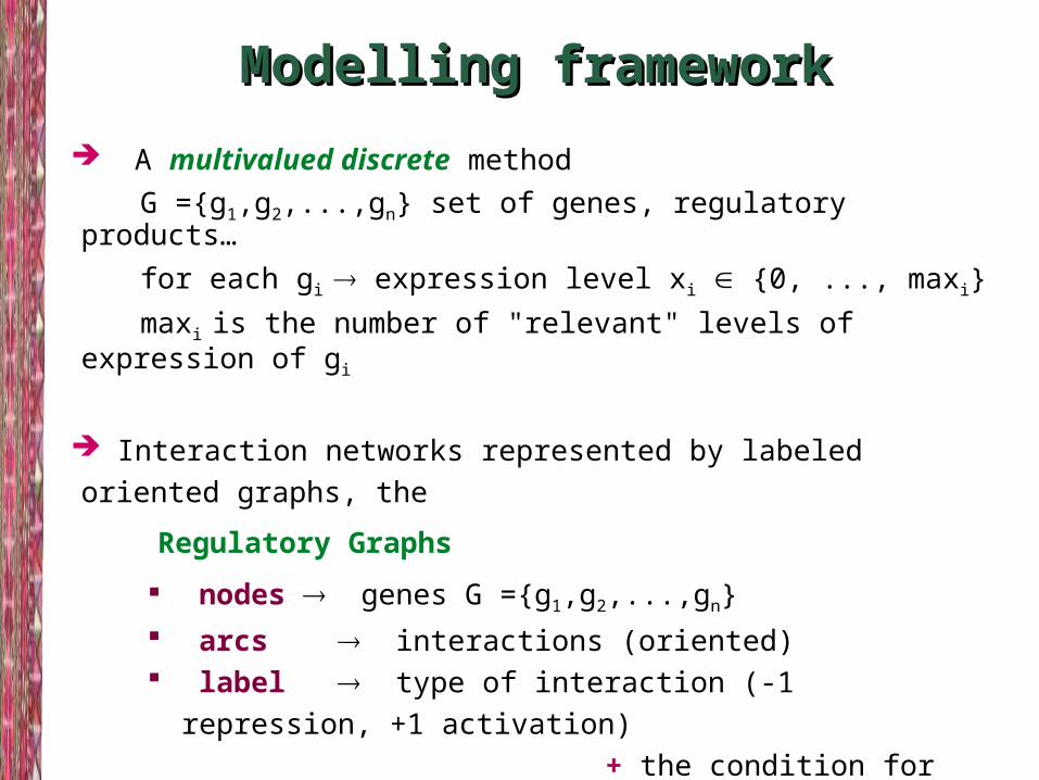
Modelling frameworkModelling framework A multivalued discrete method G ={g1,g2,...,gn} set of genes, regulatory products… for each gi expression level xi {0, ..., maxi} maxi is the number of "relevant" levels of expression of gi

Interaction networks represented by labeled oriented graphs, the

Regulatory Graphs nodes genes G ={g1,g2,...,gn} arcs interactions (oriented) label type of interaction (-1 repression, +1 activation)

+ the condition for which the interaction is operating

Modelling framework (2)Modelling framework (2)A simple illustrationA simple illustration

Interactions: T1= ( g1, g2, 1, [1])

T2=(g1,g2,-1,[2])T3=(g2,g2,1,[1])T4=(g2,g3,1,[1])T5=(g3,g1,-1,[1])

T1 T 2

T4

T5

T3

g1

g3

g2

source target type condition

Nodes Values

g1 0, 1, 2

g2 0, 1

g3 0, 1

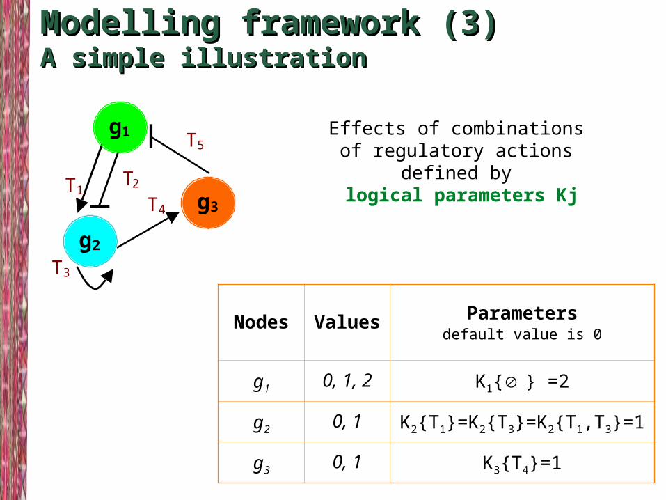
Modelling framework (3)Modelling framework (3)A simple illustrationA simple illustration

Nodes Values Parametersdefault value is 0

g1 0, 1, 2 K1{ } =2

g2 0, 1 K2{T1}=K2{T3}=K2{T1,T3}=1

g3 0, 1 K3{T4}=1

T1 T 2

T4

T5

T3

g1

g3

g2

Effects of combinations of regulatory actions

defined by logical parameters Kj

Modelling framework (4)Modelling framework (4) given x=(x1,x2,...,xn) a state, Kj(x) precises to which value gene gj

should tend if Kj(x) xj gene gj receives a call for updating

xj denotes that Kj(x) > xj call to increase

xj denotes that Kj(x) < xj call to decrease

Two dynamics: Synchronous: 100 210

Asynchronous: 100

Dynamical behaviour of the system represented by oriented graphs Dynamical Graphs

nodes states of the system arcs transitions between two "consecutive" states

+

-

200

110

++

++

Modelling framework (5)Modelling framework (5)A simple illustrationA simple illustration

Nodes Values Parametersdefault value is 0

g1 0, 1, 2 K1{ } =2

g2 0, 1 K2{T1}=K2{T3}=K2{T1,T3}=1

g3 0, 1 K3{T4}=1

+ +1 0 0

_ _

2 0 1 _ +2 1 0

0 0 0+

1 1 1_

2 0 0

_ _2 1 1

_ +2 1 0

_ _2 0 1

_ + _1 0 1

+ +1 1 0

0 0 0

0 0 1 _

1 0 0+ +

0 1 1

+A/ synchronous B/ asynchronous

T1 T 2

T4

T5

T3

g1

g3

g2

Source: Wolpert et al. (1998)

D. melanogaster :D. melanogaster :from embryofrom embryo

to adult to adult

Source: Wolpert et al. (1998)

3 cross-regulatory modules initiating segmentation

Gap Pair-ruleSegment-polarity

Anterior-Anterior-posterior posterior

patterning in patterning in DrosophilaDrosophila

Multipleasynchronous

transitions

Input:Initial maternal gradients

BCD

HBmat

BCD

HBmat

BCD

CAD CAD

Head Trunk Telson

Output:For expression patterns for the gap genes

BCD

HB

BCD

HB

BCD

CAD CAD

GT KRKNI

KR GTHB

Simulation of the Gap ModuleSimulation of the Gap Module

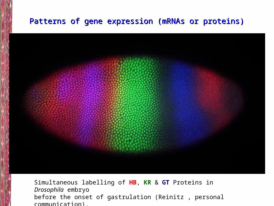
Simultaneous labelling of HB, KR & GT Proteins in Drosophila embryo before the onset of gastrulation (Reinitz , personal communication).

Patterns of gene expression (mRNAs or proteins)Patterns of gene expression (mRNAs or proteins)

Gt

Bcd

Hbzyg

Hbmat

Cad

KrKni

Maternal

Zygotic gap

Collaboration withLucas SANCHEZ (CIB, Madrid)Gap ModuleGap Module

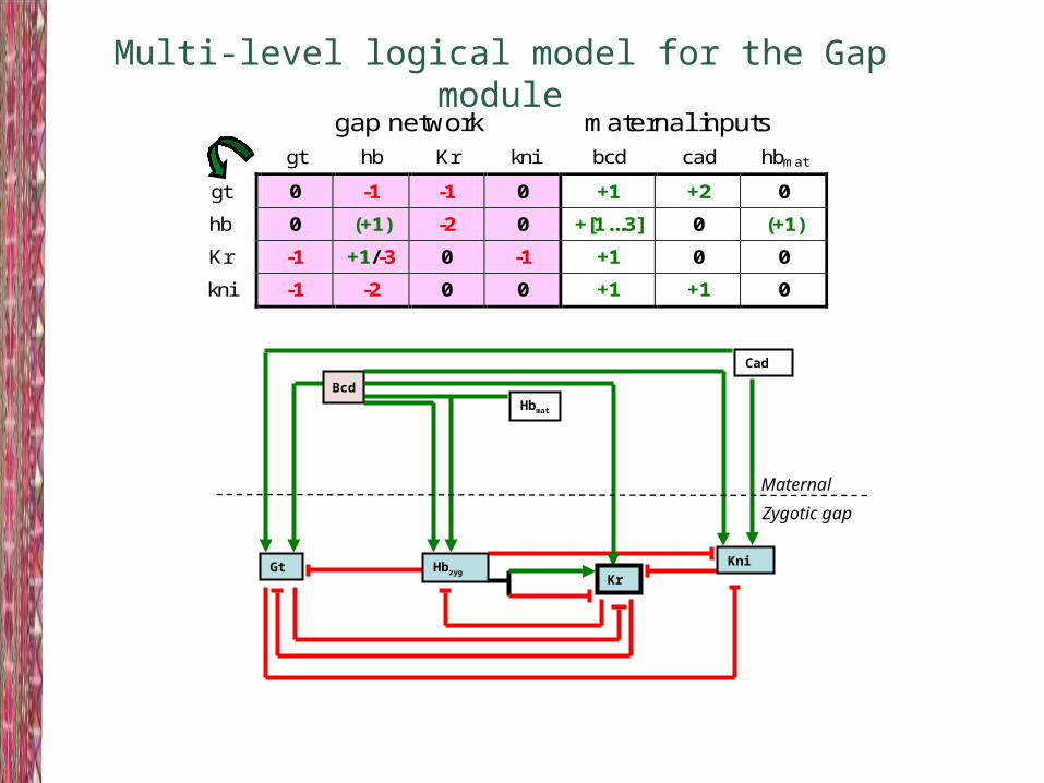
gap network maternal inputs gt hb Kr kni bcd cad hbmat

gt 0 -1 -1 0 +1 +2 0 hb 0 (+1) -2 0 +[1...3] 0 (+1) Kr -1 +1/-3 0 -1 +1 0 0 kni -1 -2 0 0 +1 +1 0

Multi-level logical model for the Gap module

Gt

Bcd

Hbzyg

Hbmat

Cad

KrKni

Maternal

Zygotic gap

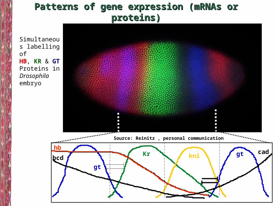
Simultaneous labelling of HB, KR & GT Proteins in Drosophila embryo

Patterns of gene expression (mRNAs or proteins)Patterns of gene expression (mRNAs or proteins)

Source: Reinitz , personal communication

gt

gthb

Kr knibcdcad

Gt KGt{Ø}=1, KGt{T3,T8}=1 Hb KHb{Ø}=3, KHb{T4}=3 Kr KKr{T5}=2, KKr{T5,T10}=1, KKr{T1,T5}=1

T10

Gt Hb

Kr

KniT2

T1

T3

T5 T6

T7

T8 T9

T4

Region A

gt

hbbcd

Regulatory graph

Patterns observed in region A Asynchronous dynamical graph

Parametrisation

Logical modelling of the GAP moduleLogical modelling of the GAP moduleSource : Sanchez & Thieffry 2001

gt, hbzyg, Kr, kni

Bcd=3, hbmat=2, cad=0 Bcd=2, hbmat=2, cad=0 Bcd=1, hbmat=0, cad=1 Bcd=0, hbmat=0, cad=2

0000

[1000] 0001+

1001-

+   +

0001

0000++ +

[0111]

0100

0110 0101

+ ++

+ +++

++

[0220]

0200+ +

0210+

[1300]

0200+++

1200 0300++ +

gt hb Kr kni

Gap Module - SimulationGap Module - Simulation ( ( gtgt,, hbhbzygzyg,, Kr,Kr, kni kni ))

gt

gthb

Kr knibcdcad

4 trunk domainsAnterior pole Posterior pole

Final state (GT, HB, KR, KNI) Genetic background

A B C D Observations/predictions

Wildtype 1300 0220 0111 1000

Bicoid 0001 0001 0001 1000 loss of GT in region A

loss of HB in ABC and of KR in BC KNI expands anteriorly into region AB

Hunchbackmat 1300 0220 0111 1000 no significant effect

caudal 1300 0220 0120 0000 increase of KR in region C

loss of KNI in region C loss of GT in region D

giant 0300 0220 0111 0001 KNI expands posteriorly into D

Krüppel 1300 1200 1100 1000 GT expands into regions B and C

Loss of KNI in region C knirps 1300 0220 0120 1000 increase of KR in region C Hunchbackmat&zyg

1000

1000

1000

1000

GT expands into regions B and C loss of KR in regions B and C

loss of KNI in region C giant-Krüppel 0300 0200 0101 0001 KNI expands posteriorly into region D Krüppel-knirps 1300 1200 1100 1000 GT expands into regions B and C giant-knirps 0300 0220 0120 0000 increase of KR in region C

Simulation of maternal and gap loss-of-function mutationsSimulation of maternal and gap loss-of-function mutations

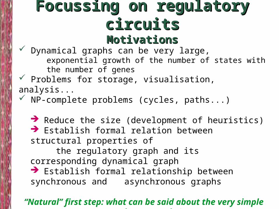
Focussing on regulatory circuitsFocussing on regulatory circuitsMotivationsMotivations

Dynamical graphs can be very large, exponential growth of the number of states with the number of genes

Problems for storage, visualisation, analysis... NP-complete problems (cycles, paths...)

Reduce the size (development of heuristics) Establish formal relation between structural properties of the regulatory graph and its corresponding dynamical graph Establish formal relationship between synchronous and asynchronous graphs

“Natural” first step: what can be said about the very simple regulatory graphs?

Focussing on regulatory circuitsFocussing on regulatory circuitsRegulatory circuits are simple structures and play a crucial role in the dynamics of biological systems :

Characteristics Positive circuits Negative circuits

Number of repressions Even Odd

Dynamical property

Biological property Differentiation Homeostasis

Simplified modelling:each gene is the source of a unique interaction and the target of a unique interaction boolean caseonly one set of parameters leads to an "interesting" behaviour (functional circuit)

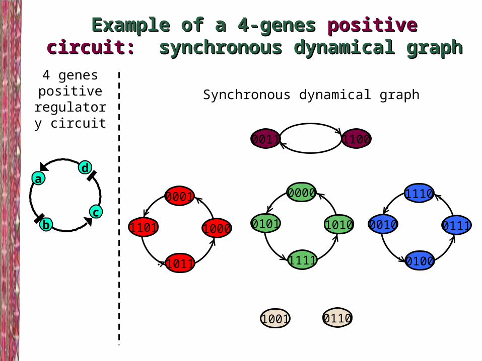
Example of a 4-genes Example of a 4-genes positivepositive circuit:circuit: synchronous dynamical graphsynchronous dynamical graph

01101001

10001101

0001

1011

11000011

10100101

0000

1111

01110010

1110

0100

d

cb

a

4 genes positive

regulatory circuit

Synchronous dynamical graph

a

d

c

b

10001101

0001

1011

10100101

0000

1111

01110010

1110

0100

01101001

k = 4

k = 2

k = 0

11000011

d

cb

a Example of a 4-genes Example of a 4-genes positivepositive circuit:circuit: synchronous dynamical graphsynchronous dynamical graph

+

+

+

--

- -

+

configuration

k=3

0111 0100

10001011

0011

k=10010

1110 1101

0001

0110 1001

0000

1111

1100

1010

0101

Example of a 4-genes Example of a 4-genes negativenegative circuit:circuit: synchronous dynamical graphsynchronous dynamical graph

d

cb

a

4 genes negative

regulatory circuit

Synchronous dynamical graph

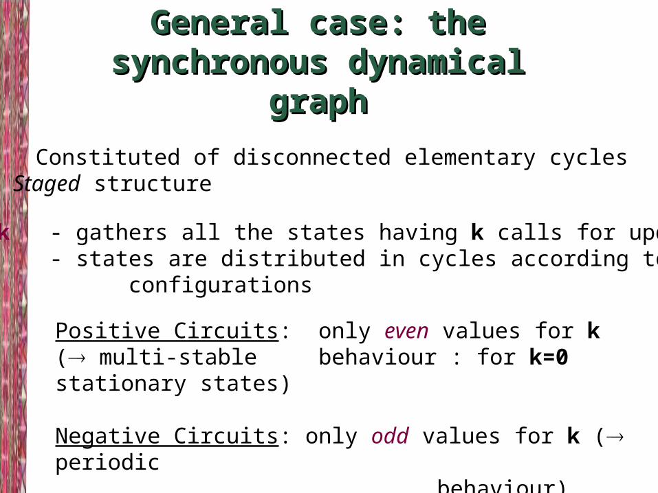
General case: the synchronous General case: the synchronous dynamical graphdynamical graph

Stage k - gathers all the states having k calls for updating - states are distributed in cycles according to their configurations

Constituted of disconnected elementary cycles Staged structure

Positive Circuits: only even values for k ( multi-stable behaviour : for k=0 stationary states)

Negative Circuits: only odd values for k ( periodic behaviour)

k=4

k=2

k=0

Example of a 4-genes positive circuit: the asynchronous dynamical graph

The synchronous version

k=4

k=2

k=0

Example of a 4-genes positive circuit: the asynchronous dynamical graph

The synchronous version

k=3

k=1

The synchronous version Example of a 4-genes negative circuit: the asynchronous dynamical graph

0010

1110 1101

0110 1001

1111

00010000

General case: the asynchronous General case: the asynchronous dynamical graphdynamical graph

Connected graph The staged structure can be conserved At stage k, each state has exactly k successors

either at the same stage k or at the stage below k-2

k=4

k=2

k=0

A compacted view of the asynchronous graphA compacted view of the asynchronous graphexample of the 4-genes positive circuit

Conclusions and PerspectivesConclusions and Perspectives Mathematical analysis

extension to more complex regulatory networks (intertwined circuits…) deeper understanding of the role of circuits embedded in regulatory networks specification of information about transition delay

Computational developments GINML: a dedicated standard XML format GINsim: a software which implements our modelling framework

Biological applications Drosophila development T Lymphocyte differentiation progressive increase of network size (~ 30 genes)