Modeling the Tail Distribution and Ratemaking: An Application of Extreme Value Theory

Jianqiang Hao, Arne Bathke, and Jerry Skees1

Selected Paper prepared for presentation at the American Agricultural Economics Association Annual Meeting, Providence, Rhode Island, July 24-27, 2005

Copyright 2005 by Jianqiang Hao, Arne Bathke, and Jerry Skees. All rights reserved. Readers may make verbatim copies of this document for non-commercial purposes by any means, provided that this copyright notice appears on all such copies. 1 Hao is a former Ph.D. student in the Department of Agricultural Economics at the University of Kentucky; Bathke is Assistant Professor in the Department of Statistics at the University of Kentucky; Skees is H.B. Price Professor in the Department of Agricultural Economics at the University of Kentucky.

1

Modeling the Tail Distribution and Ratemaking: An Application of Extreme Value Theory

Abstract

Economic analysis of weather risk often depends on accurate assessment of the

probability (P) of tail quantiles (Q). Traditional statistics mostly focuses on laws

governing the average and such methods might be misleading or biased when modeling

tail risks since the primary statistics are often driven by the data clustered in the center.

Extreme value theory can provide a promising estimation of the tail risk since it concerns

the quantification of the largest events, the smallest events, or events over the threshold in

a sample and derives the laws governing tail part events. This paper applies extreme

value theory to quantify excess rainfall across selected regions in India during the 1871 to

2001 period, and provides evidence for the feasibility and effectiveness of applying an

extreme value model in modeling and assessing weather tail risk over alternative

parametric methods.

Introduction

Economic analysis of weather risk often depends on an accurate estimation of the

probability (P) or patterns depicting the stochastic nature of a random weather variable,

especially the tail quantiles (Q). For example, accurate actuarial rates, which depend on a

precise measurement of low tail risk, are essential elements of an actuarially sound

insurance program. A few low-probability but high-consequence events often have

dominant impacts in risk assessment and thus commercial investors often use the Value-

at-Risk method to assess the portfolio risk with a low probability at the tail part.

2

Accurate ratemaking and efficient risk assessment depend on the precise

forecasting of a future occurrence, especially for the tail part risk. Technology is bringing

some certainty to predictions associated with weather events -- the field that has always

been considered unpredictable. However, until today, the most common method of

forecasting is still to use historic records of meteorological variables to derive the

probability distribution of related variables (e.g., temperature, precipitation, etc)

associated with various weather events (Podbury et al., 1998), that is, the probabilistic or

statistical method. Thus, modeling the underlying risk distribution and assessing the

impact on economic analysis are essential to weather risk management.

Considerable disagreement exists about the most appropriate characterization of

risk distributions. A variety of approaches that have been used to represent risk

distributions can be segmented into two primary groups: parametric methods and non-

parametric methods.

Under the parametric approach, a specific family of distributions (e.g., normal,

beta, gamma) is selected and parameters of this family are estimated based on the

observed data using the maximum likelihood method or the generalized method of

moments. This approach works well when the underlying population distribution family

is correctly assigned. In agriculture, parametric techniques have been extensively applied

for estimating crop-yield distributions and premium ratemaking, such as the normal

distribution (e.g., Botts and Boles, 1958; Day, 1965), the beta distribution (e.g., Babcock

and Hennessy, 1996; Kenkel, Busby, and Skees, 1991; Nelson and Preckel, 1989;

Tirupattur, Hauser, and Chaherli, 1996), the gamma distribution (e.g., Gallager, 1986),

the lognormal distribution (e.g., Jung and Ramirez, 1999; Stokes, 2000), the Su family

3

(e.g., Ramirez, Misra, and Field, 2003), and a mixture of several parametric distributions

(Goodwin and Ker, 2002). Different parametric distributions vary in terms of their

flexibility and ability to capture the crop-yield process, therefore, Sherrick, et al. (2004)

discussed the modeling of alternative distributional parameterization (i.e., the beta, the

logistic, the lognormal, the normal, and the Weibull distribution) and their economic

importance on crop insurance valuation.

Parametric techniques are also commonly used in catastrophic risk modeling. For

example, the Poisson distribution is often used to model rare and random events (i.e.,

earthquake occurrence), the Pareto distribution is used to estimate the flood frequency or

fire loss, and the lognormal distribution is frequently used to track the earthquake motion,

raindrop size, or Tornado path (Woo, 1999).

The prerequisites of functional form and distribution assumptions for the

parametric approach may result in an imprecise prediction and misleading inference

when the underlying distribution choice is incorrect. That is, parametric methods are

susceptible to specification errors and their statistical consequences.

Nonparametric methods have been developed for the situation where we do not

assume any knowledge of a specific distribution family of the underlying population. The

simplest nonparametric technique is the histogram and the most commonly used

nonparametric methods are based on the empirical distribution. Compared to the

parametric approach, the nonparametric approach is free of functional forms and

distribution assumptions (distribution free) and relatively insensitive to outliers.

Therefore, this approach is impervious to specification errors and might result in more

accurate and robust models (Featherstone and Kastens, 1998). However, some

4

nonparametric procedures (e.g., the kernel procedure) have a relatively slow rate of

convergence to the true density (Silverman, 1986) and a potential difficulty in measuring

rare events. Some efficiency might also be lost when prior knowledge of the underlying

distribution form is available. Furthermore, it is problematic to use the nonparametric

approach in analyzing multiple variables with small samples.

In agriculture, in addition to the empirical distribution and histograms, a variety of

kernel functions have been used in estimating crop-yield distribution and rating crop

insurance contracts, such as Turvey and Zhao (1999), Goodwin and Ker (1998), Ker and

Goodwin (2000), and Ker and Coble (2003).

Traditional statistics, including both parametric and nonparametric methods,

mostly focus on the laws governing averages. Basic statistical measures of risk are all

based on the centered data. When modeling weather risk, our interest is not in estimating

the whole distribution but the tail risk. The use of standard parametric or nonparametric

methods might be misleading or biased in modeling the tail risk since the primary

statistics are driven by the data clustered in the center. This bias can further cause

imprecise ratemaking when designing a weather-based contingent claims. To overcome

the disadvantage of applying standard methods in modeling tail risk, extreme value

theory could provide a promising solution since it is primarily concerned with the

quantification of the stochastic behavior of a process at usually the largest, the smallest,

or the events over a threshold in a sample and derives the laws governing tail events.

This paper applies statistical techniques to quantify weather tail risk and compares

the results from standard statistical distributions with an innovative approach – extreme

value theory with risk estimation and premium setting. The objective of this essay is to

5

provide evidence for the feasibility of applying extreme value models in modeling

weather tail risk and investigating its effectiveness over other alternative distributions on

economic importance of premium ratemaking and risk assessment. Four parts are

included in this essay. First, the essentials of tail distribution estimation is emphasized for

modeling and assessing weather risk in the first part; Secondly, the statistical model for

modeling the tail distribution – extreme value theory - is introduced along with the

statistical properties; The third part develops a research procedure that compares the

estimation and actuarial performance of the standard distributions and the extreme value

model using monthly rainfall data across different regions in India over the period from

1871 to 2001. The power and efficiency of the Extreme Value Model are further

demonstrated by modeling the tail risk. Finally, conclusions and recommendations are

developed.

Tail Estimation -- Let the tails speak for themselves!

Traditional statistics mostly looks at the laws governing the average. Basic

statistical measures of risk, mean, variance, and the third or fourth central moments, are

all based on the center of the observed data. For example, consider a sample of n

observations, iy , for i=1 to n. The population mean is estimated from the sample

average, i.e., ∑=

=n

iiy

ny

1

1 ; The population variance that is used to measure the spread of

the distribution is estimated by the sample variance ∑=

−−

=n

ii yy

ns

1

22 )(1

1 ; The

skewness is used to measure the symmetry of the distribution. The sample estimate of the

skewness is 31

3

)1(

)(

sn

yya

n

ii

−

−=∑= ; The kurtosis is based on the fourth central moment, which

6

is a measure of the “peakiness” of the distribution. The sample estimate of the kurtosis is

41

4

)1(

)(

sn

yyk

n

ii

−

−=∑= . It is obvious that the basic statistical measures of risk are all based on

the center of the data ( y ), and they may not be able to truly reflect the tail characteristics.

However, in weather risk estimation, a few low probability events will exert a

high, or even dominant impact on risk assessment and the quantification of (P, Q)

combinations needs to rely on the (asymptotic) form of tail distribution. Estimation and

inference based on the whole distribution might be inaccurate since the data clustered in

the center of the distribution will have too much influence over the estimators.

Misspecification of the distribution family can, in turn, bias the calculation of the

insurance premiums and indemnity payments.

The reasons behind applying tail estimation are summarized as follows: 1) Model

estimation and assessment of the model fit using standard statistical procedures are often

driven by the centered values of the data; 2) A trend in frequency or magnitude might be

confined to one or both tails of a distribution; 3) Alternative distributions that fit the

observed data well might have different performance in a tail estimation; 4) Accurate

ratemaking of weather contracts relies on tail part estimation.

Recently, some researchers (e.g., Ker and Coble, 2003) have noticed this problem

and suggest modeling the conditional risk distribution instead of the whole distribution in

risk assessment. However, the risk estimation and economic analysis of alternative

distribution specifications on modeling conditional weather risk have not been well

documented. Specifically, the performance of alternative distributions on conditional tail

part risk valuation has not been addressed in most of the literature.

7

Extreme Value Model

Extreme value theory (EVT) dates back to the late 1920s to early 1940s following

the pioneering work of Fisher and Tippett (1928), and Gnedenko (1943). In 1958 Gumbel

laid out the theoretical framework of the extreme value model in his classical book.

Extreme value techniques have been extensively applied in many disciplines during the

last several decades, including meteorology (e.g., wind speeds, ocean wave,

precipitation), engineering (e.g., quality control, wind engineering, alloy strength

prediction), catastrophic phenomena (e.g., thermodynamics of earthquakes, floods,

storms, hurricanes), and non-life actuaries (e.g., risk assessment, loss estimation). From

the early 1990s, applications of EVT in modeling financial extremes have become more

and more popular, especially measuring Value at Risk (VaR) on the tails of the Profit &

Loss (P&L) distribution (Chen and Chen, 2002).

Generally, there are two principal kinds of approaches in modeling extreme

values, the block maxima model (BMM) and the peak over threshold model (POT). The

first approach models the largest or the smallest values for a series of identically

distributed observations. For example, annual maximum sea level, the fastest race times

in sport, daily minimum temperature, the largest claim in insurance, etc. This approach

can be further extended to model the (r) largest order statistics. On the other hand, the

peak-over-threshold approach models all large (small) observations that exceed (fall

below) a high (low) threshold. This approach might be more useful for practical

applications since it is more efficient to use limited resources on extreme values instead

of only the largest or smallest observation. In some realistic situations, the extreme value

8

approach may involve a loss of information and the accuracy of estimation of a small

sample size might be compromised.

Block Maxima Model (BMM)

The BMM approach focuses on the statistical behavior of the largest or smallest

value in a sequence of independent random variables. In modeling weather risk and

designing an efficient risk management system, it might be of particular interest when

asking such a question as: “What is the probability that the maximum event for next year

will exceed all previous levels?” In the actuarial industry, such information might be

especially important in determining the buffer fund and probability of ruin that can

jeopardize the position of the insurance or reinsurance company due to catastrophic loss.

Statistically, assume nM be the maximum of the process over n independent

random variables with a common distribution function F.

},,max{ 1 nn XXM L=

In theory, the distribution of nM can be derived by

(1) nnn zFzXzXPzMP )}({},,()( 1 =≤≤=≤ L

Since the exact distribution of nM depends on F(z) which is unknown, the

asymptotic distribution of nM is of particular interest. However, 0)( →zF n as ∞→n ,

the distribution of nM degenerates to a point. Thus, the extreme value ( )nM needs to be

normalized in order to have a non-degenerate limiting distribution.

(2) n

nnn a

bMW −=

where nb (>0) and na (>0) are the location and scale parameters respectively.

9

The Fisher-Tippet Theorem proves the existence of the limiting distribution of the

normalized extreme value nW .

(3) )()(lim zGza

bMPn

nn

n=≤

−∞→

where G is a non-degenerate distribution and a generalized extreme value (GEV)

family can be used to capture the above distribution.

(4) })](1[exp{)( /1 ξ

σμξ −

+−

+−=zzG

Here, μ and )0(>σ are location and scale parameters, and ξ is a shape

parameter. Three families of limit distributions can be obtained from the GEV family:

I (Gumbel): ∞<<∞−−

−−= zzzG )]},(exp[exp{)(σμ as 0lim →ξ

II (Frechet): ⎪⎩

⎪⎨⎧

>−

−

≤= − μ

σμ

μξ zforz

zforzG },)(exp{

,0)( as 0>ξ

III (Weibull): ⎪⎩

⎪⎨⎧

≥

<−

−=−

μ

μσμ ξ

zrfo

zforzzG

,1

},)(exp{)( as 0<ξ

The GEV family can be easily transformed to modeling the smallest value by

changing the sign. Assume },,min{ 11 nXXM K= , let ii XY −= and },,max{ 1 nn YYM K= ,

then 1MM n −= and nM can be fitted by the GEV family. The maximum likelihood

estimate of the parameter )ˆ,ˆ,ˆ( ξσμ for the asymptotic distribution of nM corresponds

exactly to that of the asymptotic distribution of 1M , except for the sign change of the

location parameter. Furthermore, the GEV family can be extended to model the rth largest

or smallest order statistics and the parameters of the GEV family can be estimated in the

10

presence of covariates, such as trends, cycles, or actual physical variables (e.g., the

Southern Oscillation Index in the rainfall process).

Maximum likelihood procedures can be employed to estimate the GEV

parameters ξσμ ,, . These estimators are unbiased, consistent, and asymptotically

efficient. Although there is not always a straightforward analytical solution, the

estimators can be found using standard numerical optimization algorithms.

Peak over Threshold Model (POT)

Modeling only maxima or minima can only be applied when the particular interest

is in the largest or smallest event, and this method is also an inefficient approach if other

data on the tail are available and of interest. Therefore, the BMM approach is too narrow

to be applied to a wide range of problems. Generally, a question such as “what is the

probability that the occurrence of the next event will exceed a predetermined level u

(threshold)?” is more useful for weather risk analysis.

POT can compensate such shortcomings and be used to model all large (small)

observations that exceed (fall below) a high (low) threshold. These exceedances are

important in determining the insurance or reinsurance premium rates, claims, buffer fund,

ruin probability, and may even be helpful when design preventive strategies for risk

management.

Let’s assume u is the threshold and the tail events are regarded as those of iX that

exceed u }},,{ 1 uXX r >L . Then the stochastic behavior of these events whose values

are greater than the pre-specified threshold value u can be represented by the following

conditional probability function.

11

(5) 0,)(1

)(1)|( >−

+−=>+> y

uFyuFuXyuXP

)(1)()(

)(1)()()|()(

uFuFrF

uFuFyuFuXyuXPyF

−−

=−

−+=>≤−=μ

Where r denotes these excess of iX above u and F is the marginal distribution of

the sequence of random variables Xi..

Pickands (1975), Balkema and de Haan (1974) have shown that if block maxima

have an approximate GEV distribution, then threshold excesses have a corresponding

approximate distribution within the Generalized Pareto Distribution family (GPD) and

the parameters of GPD are uniquely determined by those of the associated GEV

distribution of block maxima. For a large enough threshold u , the distribution function

of )( uX − conditional on uX > can be approximated by

(6) ξ

σξ /1)1(1)( −+−=

u

yyH

where )( μξσσ −+= uu

If 0<ξ (Weibull), the distribution of excesses has an upper bound; If

0>ξ (Frechet), the distribution of excesses has no upper limit. If 0→ξ (Gumbel), the

distribution can be simplified. It is exactly an exponential distribution with

parameter uσ/1 .

Similar to the GEV distribution, maximum likelihood procedures can be utilized

to estimate the GPD parameters given the threshold u.

The determination of the threshold u is crucial to perform the POT method. There

exists a tradeoff between bias and variance in determining the threshold. For example,

too low a threshold is likely to violate the asymptotic basis of the model and may lead to

12

a bias; too high a threshold will generate too few observations left to estimate the

parameters of the tail distribution function and may cause high variance. Coles (2001)

suggests adopting as low a threshold as possible, subject to the limit model providing a

reasonable approximation. Graphically, the mean residual life plot and Hill-plot (Coles,

2001; Chen, 2002) can be performed to determine the crucial threshold u. The goodness-

of-fit test suggested by Gumble (1958), and the Bootstrap methods suggested by Dekkers

and de Haan (1989) can also be used to approach this problem.

Whether the fitted models are good enough to model the observed data is

particularly important in statistical inference. Probability plots, quantile plots, and return

level plots are often used to assess the quality of fitted GEV and GPD models. Details

concerning the extreme value theory can be found in Coles (2001), and Embrechts,

Kluppelburg and Mikosch (1997).

Research Design

This study provides an empirical analysis of modeling weather risk using

alternative parametric distributions and extreme value theory. Premium rates of a

hypothetical weather index with varying strikes are calculated and a statistical

comparison is performed.

Data

Indian agriculture accounts for 24 percent of the GDP and provides work for

almost 60 percent of the population. Monsoons in India can bring damaging cyclones and

floods to the coastal plain. Heavy flooding in 2000 caused about 1,200 deaths in Southern

India and Bangladesh (Swiss Re, 2001). Officials in Andhra Pradesh reported that by

August 30, 2000 the floods had affected 3,080 villages and towns and submerged

13

177,987 hectares of farmland, causing damage officially estimated at 7.7 billion rupees.

The real destruction far exceeded these figures.2

Parchure (2002) estimates that about 90 percent of the variation in the crop

production of India is due either to inadequate rainfall or to excess rainfall. Generally,

excess rain is concentrated in the months of June to September. However, the

performance of the current crop insurance program in India can be considered

disappointing (Kalavakonda and Mahul, 2003; Mishra, 1996; Parchure, 2002; Skees and

Hess, 2003), and developing rainfall-based insurance can be considered an economically

viable instrument. For example, Veeramani, Maynard and Skees (2003) suggest rainfall-

based indices and options as a replacement for the current expensive area crop-yield

programs for Indian rice farmers.

In this study, historic monthly rainfall from the months of June to September over

1871 to 2000 period is used across fourteen different subdivisions. The data is collected

from the Indian Institute of Tropical Meteorology.

The use of time series data to estimate an underlying distribution needs the data to

be identical and independent, thus a series of tests are necessary.

1) Deterministic trend or stochastic trend

The augmented Dickey Fuller (ADF) and Phillips-Perron (PP) tests were used to

test for the existence of a stochastic trend on a region-by-region basis. All of the fourteen-

rainfall series were found to be trend stationary and the unit root tests were rejected in all

cases. The results suggest that a deterministic trend might be appropriate for the rainfall

series.

2) Linear trend or higher order trend 2 Source: http://www.wsws.org/articles/2000/sep2000/ind-s06.shtml

14

The possible trend order was examined by regressing time series rainfall data

against a possible time trend (e.g., linear, quadratic, cubic, or higher order) based on the

significance of the F-test. Greene (2003) notes the conservative nature of this test in cases

of non-normal errors.

The results indicated that only two of the fourteen regions were found to have

significant linear trends (Region COAPR with a 10% significant level and Region

SASSM with a 5% significant level). Region TELNG has a significant quadratic term

and a fifth order term at the 10% level and the fourth term at the 5% level. Regions

WMPRA and SHWBL have significant cubic terms at the 5% level and the 10% level,

respectively. But none of them have significant lower order terms.

3) Autocorrelation and Normality

Durbin-Watson tests are used to indicate the incidence of the first order

autocorrelation for lag one series (monthly autocorrelation) and lag four series (yearly

autocorrelation). The results showed that the DW test was only rejected in one region,

SASSM, at a 5% significant level. A normality test3 failed to reject in only one region,

NASSM, at a 5% significant level and in two regions, BHPLT and SASSM, at a 10%

significant level. Since only two regions have a deterministic trend (CORPA and

SASSM), a heteroscedasticity test is not performed in this study.

Given the sporadic violations of the i.i.d. assumptions, a linear trend was imposed

for regions COAPR and SASSM and the time series rainfall data were detrended by a

linear term to a base year of 2001. The raw rainfall data were used for the twelve other

regions. The summary statistics of rainfall data are shown in Table 1.

3 the Kolmogorov-Smirnov test.

15

The mean of monthly cumulative rainfall during the period from June to

September across the fourteen regions average 2800mm, indicating that excess rainfall

can be a significant risk. The sample means vary considerably ranging from a low of

1784mm (TELNG) to a high of 5014mm (SHWBL). Sample medians are slightly smaller

than sample means in all regions except EUPRA and NASSM, ranging from 1707mm

(TELNG) to 4896mm (SHWBL) with an average of 2736mm. The variability of monthly

rainfall is also different across the regions, with standard deviations ranging from 779

(TELNG) to 1655 (SHWBL). The coefficients of skewness range from 0.139 (EMPRA)

to 0.743 (TELNG), with an average of 0.41 across all regions. Positive skewness calls

into question the use of symmetric distribution (e.g., normal distribution) to model

rainfall. The coefficients of sample kurtosis range from -0.905 (WUPRL) to 0.783

(TELNG), with an average of -0.089. Both negative kurtosis (sub-Gaussian) and positive

kurtosis (super-Gaussian) appear across the different regions, showing the possibility of

both “less peaked” and “more peaked” density functions. Monthly cumulative rainfall

levels vary significantly across regions. For example, the maximum rainfall ranges from

as low as 4894mm in COAPR to 10129mm in SHWBL; the minimum rainfall fluctuates

from 4mm in WUPRL to 1531mm in SASSM. The summary statistics indicate that

rainfall across regions displays significantly different distributions but predominantly

positive skewness.

Research Procedure

Our interest is to provide evidence for the feasibility of applying the extreme

value theory in modeling weather tail risk and to investigate its efficiency over other

alternative distributions on economic importance of premium ratemaking and risk

16

assessment. Therefore, the focus is to compare the statistical estimation and premium

ratemaking based on standard statistical methods and extreme value theory. In this study,

four alternative distributions are selected as the parametric candidates and the GPD

model is chosen as the extreme value candidate. Our research procedure includes the

following five steps.

Step 1. Estimate the rainfall series using parametric distributions

Four parametric distributions, including the beta distribution, the gamma

distribution, the lognormal distribution, and the Weibull distribution, are chosen as

parametric candidates, and the maximum likelihood method is used to estimate the

parameters. The actuarially fair premium rates were further calculated for a hypothetical

weather-based contingent claim based on these four candidate distributions.

Step 2. Rank parametric candidates

For each of the fourteen rainfall series, four parametric candidates are ranked

from the best to the worst based on several goodness of fit tests (e.g., the Kolmogorov-

Smirnov test, the Cramer-von Mises test, the Anderson-Darling test, and the Chi-Square

test) and the visual QQ plot. The weighted rank for each candidate is further calculated.

Step 3. Estimate the rainfall series using EVT model

The GPD model is chosen to estimate the excess rainfall distribution for each

region and an actuarially fair premium rate is calculated further for the weather-based

contingent claim.

17

Step 4. Compare the economic importance of estimations based on two methods

The calculated premium rates from the extreme value theory and the best

candidate from the standard statistical distributions are tested for equality of mean using a

couple of nonparametric paired tests, e.g., the sign test and the Wilcoxon signed rank test.

Step 5. Sensitivity analysis of different strike levels

Different feasible strikes are applied and the robustness of our results is then

discussed through the sensitivity analysis.

Fitting the Alternative Parametric Distributions

Parametric techniques fit the observed data to one of the standard distributions

(e.g., the beta distribution, the gamma distribution, etc) by some statistical methods (e.g.,

by the maximum likelihood method or the generalized moment method). In selecting the

parameterization of rainfall distributions, several considerations were given to 1) Stylized

features of cumulative rainfall (i.e., non-negativity, skewness); 2) Flexible parameters to

adequately characterize cumulative precipitation over time periods across different

regions; 3) Previous studies and empirical evidence from climatological, hydrological,

and agronomical research (Barger and Thom, 1949; Thom, 1958; Ison, et al., 1971;

McWhorter, et al., 1966). Four candidate distributions are considered in this study: the

beta distribution4, gamma distribution, lognormal distribution, and weibull distribution.

Maximum likelihood methods were applied to solve for the parameters of the four

distributions for each region sample. The log-likelihood functions and MLEs for the

gamma distribution are illustrated as follows. The likelihood function for the parameters

of the gamma distribution can be specified as follows:

4 The upper bound parameter, to guarantee x to be between zero and one, was set to 5% above the maximum rainfall recorded in this study.

18

(7) βααβα

βαβα /1

11

)()(1),;();,( ∑

Γ== −−

==∏∏ ix

n

iinn

n

ii exxfxL

The log-likelihood function to be maximized is written as

(8) βαβααβα /log)1(log))(log();,(11∑∑==

−−+−Γ−=n

ii

n

ii xxnnxLogL

βα , can be obtained from the first derivative of the above equation and MLEs of

βα , are unbiased, consistent and asymptotically efficient.

If any of the cumulative precipitation observations in the historical data serials are

equal to zero, a censoring estimation suggested by Wilks (1990), and Martin, Barnett and

Coble (2001), could be applied. The log-likelihood function for the censoring function

can be written as

(8’) βαβαβαβα /)1(]log))([log()],;(log[);,(11∑∑==

−−++Γ−=n

ii

n

iiwC xxnNCFNxLogL

Where C is the censoring point, for example, a small number C=0.01 inch; Nc

denotes censored years in which cumulative precipitation over the contract time is

recorded as zero; Nw denotes non-censoring years; and N = Nc + Nw.

The parameters for all four distributions were estimated separately using the

rainfall data from region a, and then for region b, and so on through each sample. The

summary statistics of the four candidate distributions are provided in Table 2. The results

further indicate that the distributions differ meaningfully across regions.

Rank Alternative Distributions

Each of the alternative distributions has two parameters to be estimated in this

study and we thus have the same degrees of freedom when performing the maximum

likelihood functions for the rainfall series.

19

Alternative distributions can be ranked for the goodness-of-fit according to some

standard tests and visual QQ plot. SAS 8.2 provides several goodness-of-fit tests for the

appropriateness of candidate distribution, such as the Kolmogorov-Smirnov test, the

Cramer-von Mises test, the Anderson-Darling test, and the Chi-Square test. Under each

test, the null hypothesis is set as: The empirical distribution is equal to the best candidate

within the respective parametric family of distributions. A large p-value fails to reject the

null hypothesis suggesting that the candidate distribution might be appropriate to fit the

sample data. However, these goodness-of-fit tests are not optimal for comparing the tail

behavior of the distributions. Therefore, also QQ plots have been generated.

The QQ plot provides the visual evidence for the goodness-of-fit of the candidate

distribution. If F̂ is a reasonable model for the population distribution, the quantile plot

should be close to the unit diagonal. Since there is particular interest in the goodness-of-

fit of the tail part risk rather than the whole distribution, the QQ plots may be more

appropriate than the standard tests when assessing the performance of the tail part

estimation.

Based on the standard goodness-of-fit tests and QQ plot, we can rank the

appropriateness of the four distributions in fitting the rainfall series for each region. The

following example illustrates how to rank alternative distributions for the rainfall series

using the region of WMPRA. The plot of alternative distributions is shown in Figure 1.

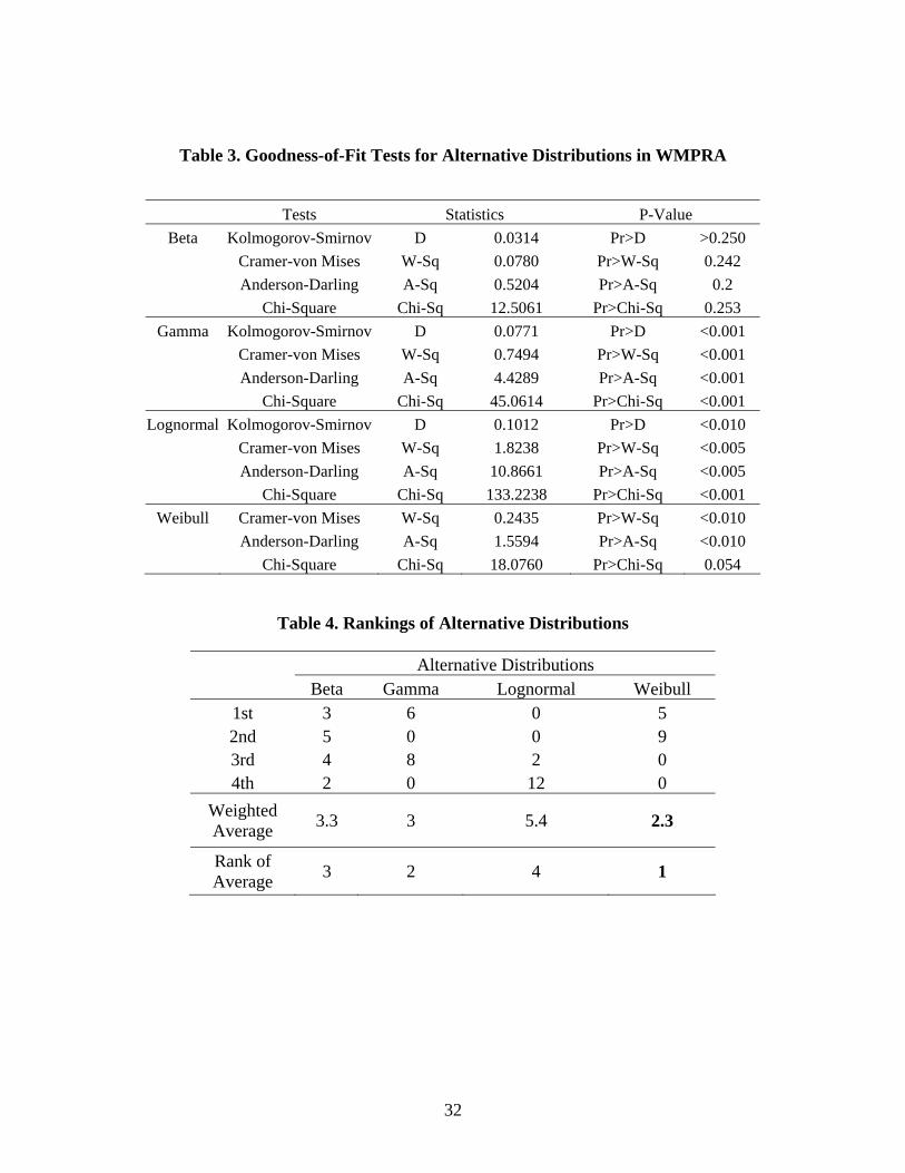
The statistics of standard goodness-of-fit tests are reported in Table 3. QQ plots of

alternative distributions are provided in Figure 2.

Both the QQ plot and the standard goodness-of-fit tests suggest that the beta

distribution should be the most appropriate candidate in modeling the rainfall series since

20

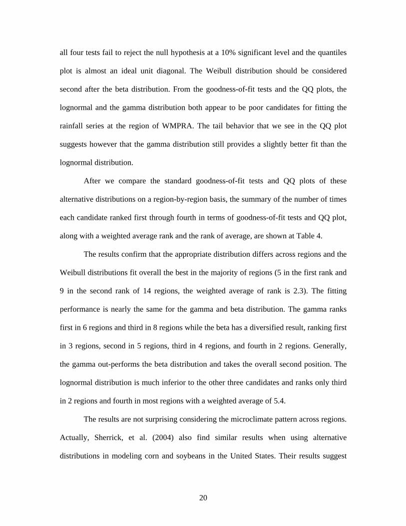
all four tests fail to reject the null hypothesis at a 10% significant level and the quantiles

plot is almost an ideal unit diagonal. The Weibull distribution should be considered

second after the beta distribution. From the goodness-of-fit tests and the QQ plots, the

lognormal and the gamma distribution both appear to be poor candidates for fitting the

rainfall series at the region of WMPRA. The tail behavior that we see in the QQ plot

suggests however that the gamma distribution still provides a slightly better fit than the

lognormal distribution.

After we compare the standard goodness-of-fit tests and QQ plots of these

alternative distributions on a region-by-region basis, the summary of the number of times

each candidate ranked first through fourth in terms of goodness-of-fit tests and QQ plot,

along with a weighted average rank and the rank of average, are shown at Table 4.

The results confirm that the appropriate distribution differs across regions and the

Weibull distributions fit overall the best in the majority of regions (5 in the first rank and

9 in the second rank of 14 regions, the weighted average of rank is 2.3). The fitting

performance is nearly the same for the gamma and beta distribution. The gamma ranks

first in 6 regions and third in 8 regions while the beta has a diversified result, ranking first

in 3 regions, second in 5 regions, third in 4 regions, and fourth in 2 regions. Generally,

the gamma out-performs the beta distribution and takes the overall second position. The

lognormal distribution is much inferior to the other three candidates and ranks only third

in 2 regions and fourth in most regions with a weighted average of 5.4.

The results are not surprising considering the microclimate pattern across regions.

Actually, Sherrick, et al. (2004) also find similar results when using alternative

distributions in modeling corn and soybeans in the United States. Their results suggest

21

that the Weibull and beta distributions are overall ranked first and second in fitting corn

yield and the logistic and Weibull distributions perform first and second in modeling

soybean yield for selected farms at the University of Illinois.

Distributional choice has a tremendous impact on the risk assessment and the

selection of an appropriate underlying distribution can directly determine the economic

effectiveness of risk hedging. Since the appropriate distribution differs across regions due

to microclimate patterns, it might be best to find an appropriate candidate for each region

based on the specification tests. However, such a method is time-consuming and costly

for a large area. For example, crop-yield distributional modeling involves thousands of

counties in the United States and rainfall series estimation includes hundreds of regions

in most developing countries. Therefore, it is common to adopt the overall best

distribution used in current crop insurance programs and weather index design.

Unfortunately, even the overall best distribution can lead to misleading risk assessments

and inaccurate premium ratemakings in some regions. For example, the Weibull

distribution ranked best overall but only fitted best in 5 regions. We might lose some

efficiency in the other 9 regions when applying the Weibull distribution to model the

rainfall series across regions.

Fitting the POT Model

The EVT model is considered a promising alternative when modeling tail risk and

can be applied in weather risk modeling when designing a weather-based contingent

claim. In this part, the POT model is used to model the excess rainfall risk and the GPD is

chosen as the candidate distribution.

22

First, the threshold (u) is decided, based on the mean residual plot on a region-by-

region basis. As discussed earlier, an ideal mean excess plot should be approximately a

straight line against the threshold. Next, the scale and shape parameters are estimated by

the maximum likelihood method, based on the procedures provided above. Finally, a

variety of statistical techniques, such as the PP plot, the QQ plot, the return level, and the

density function, are plotted to check the appropriateness of the GPD in modeling excess

rainfall. The parameters of GPD across regions are provided in Table 5.

Since the estimated shape parameter is 0ˆ <ξ for all regions, the excess monthly

rainfall follows the type III class of extreme value distribution, that is, the Weibull

distribution. The various diagnostic plots for assessing the appropriateness of the GPD

model fitted to the rainfall data across regions. None of these plots calls into question the

validity of the fitted models.

Weather Index Design and Premiums Ratemaking

A weather derivative is a contract between two parties that stipulates how

payment will be exchanged between the parties depending on certain meteorological

conditions during the contract period. Zeng (2000) suggested that seven parameters

should be specified for a weather derivative contract: 1) Contract type (call or put); 2)

Contract period; 3) An official weather station from which the meteorological record is

obtained; 4) Definition of the weather index underlying the contract; 5) Strike; 6) Tick or

constant payment for a linear or binary payment scheme; 7) Premium.

Weather-based contingent claims provide a cross-hedging mechanism against the

variability of a firm’s revenue or costs. For example, extreme heat or excess humidity can

cause increased death for livestock and/or higher cooling costs. Therefore, a contingent

23

claim based on THI (temperature-humidity-index) can provide a viable, though not

perfect, cross-hedging mechanism for livestock producers.

The contract should have a relatively simple structure but be flexible enough to

capture adequate coverage and protection. In this study, the design of the weather index

follows the European precipitation options proposed by Skees and Zeuli (1999) but it is

in the form of call options, that is, indemnity payments are triggered when the actual

monthly precipitation is above the pre-specified strike. The indemnity function is given

by

(9) )0),(()~(c

c

xxXMaxwI −

×= θ

where cx is the the predetermined trigger for obtaining the indemnity. and θ is the

the liability, that is, the maximum possible indemnity.

To formalize this study, the strike cx is defined as a fraction of the proven

precipitation level, x 5, that is,

(10) xhxc *=

The available fractions of proven precipitation vary from 1.2 to 1.5 in this study.

The pure premium rate is the standard basis for establishing insurance actuarial policy

and can be calculated based on the expected loss cost using a time series of historical

data. Here, the break-even premium rate can be calculated as the average of the

percentage shortfalls above the strike following Skees, Barnett and Black (1997) and Ker

and Coble (2003).

(11) c

cccw i

c

ci x

xxxXExXPxdFx

xXPc

))|()(()()( −>>=

−=∫

∞

5 In this study, the mean of monthly rainfall during 1871 to 2001 is chosen as the proven precipitation level.

24

where the expectation operator and probability measure are taken with respect to

the underlying distribution (i=1 means the beta distribution, i=2 means the gamma

distribution, i=3 means the lognormal distribution, i=4 denotes the Weibull distribution,

and i=5 denotes GPD).

Therefore, given a risk distribution and strike level, the pure premium rates can be

easily obtained from Eqn (11). Table 6 reports actuarially fair premium rates estimated

for each region across five rainfall distributions with varying strike levels. The paired t-

tests for equality of means of alternative parametric distributions and GPD are also

provided in this table.

Among the four alternative distributions, the Weibull distribution, the overall best

fitting candidate, tends to have lower pure premium rates while the lognormal

distribution, the overall worst fitting candidate, tends to have higher premium rates. Due

to the diversified performance of the beta and gamma distribution, the pure premium

rates obtained from these two candidates are generally between the lowest level obtained

from the Weibull distribution and the highest level obtained from the lognormal

distribution. The results suggest that some parametric distributions might underestimate

the tail risk (i.e., the Weibull distribution) while other might overestimate it (i.e., the

lognormal distribution). On the other hand, the pure premium rates obtained from the

GPD lie in-between those from the Weibull distribution and those from the beta and

gamma distributions, suggesting that the GPD might be more appropriate in modeling tail

part risk. However, further statistical tests are needed.

The strike levels that trigger the indemnity payment vary when h equals 1.2, 1.3,

1.4, and 1.5, respectively. The premium rates tend to be lower with a higher strike and

25

higher with a lower strike level. Furthermore, paired t-tests are performed where the GPD

is chosen as the reference sample. The results show that the premium rates obtained from

the Weibull distribution at h =1.5 and h=1.2, and the beta distribution at h=1.2 are

insignificant from those obtained from the GPD. Others are all significant different than

those obtained from the GPD. The results suggest that alternative candidates have

significantly different performances in economic implications.

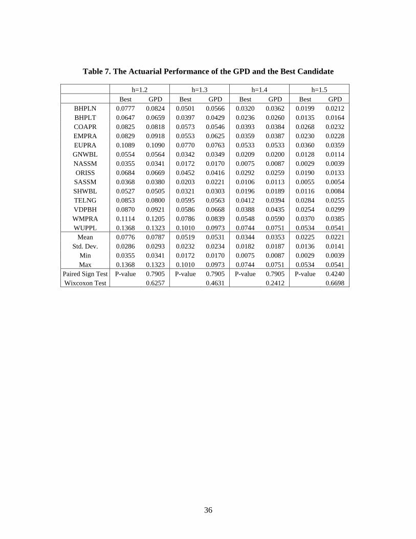
Next, we compare the premium rates from the GPD and those from the first

ranked candidate based on the goodness-of-fit test and the Q-Q plot. For each region, the

pure premium rate based on the best candidate among the beta distribution, the gamma

distribution, or the Weibull distribution, is chosen as the base case and compared with the

performance of the GPD in modeling the tail risk. Nonparametric sign test and Wilcoxon

signed rank test are applied to test the equality of means and Table 7 shows the results.

The means and variability of pure premium rates from the GPD are very close to

those from the best candidate across different strike levels. Furthermore, all of these tests

fail to reject the null hypothesis of the equality of pure premium rates based on the GPD

and the best candidate with a high p value, demonstrating that the GPD performs as good

as the best standard parametric method, and it is effective and robust in modeling and

assessing tail risk, and premium ratemaking

Conclusion

Accurate estimation of tail events may be of particular interest to decision makers.

The EVT can be considered the-state-of-the-art procedure for estimating the downside

risk of a distribution and provides promising potential for risk assessment and premium

ratemaking of weather-based contingent claims.

26

The results also demonstrate that large differences in actuarially fair premium

rates for a rainfall-based contingent claim can arise solely from the parameterization

chosen to represent the underlying risk distributions and misspecification in the risk

distribution (e.g., the lognormal distribution) may lead to economically significant errors

in weather index premium ratemaking and assessment of expected risks.

Furthermore, when modeling the tail risk, the GPD model is promising since it

performs close to the best candidate chosen by different parametric distributions. What is

evident from this study is that the distributional choice has a significant impact on rating

and assessing weather-based contingent claims, and so the GPD model might be effective

in modeling the tail risk.

However, this study addresses a limited set of parametric distributions and only

one potential weather-based contingent claim (the rainfall index). Future work could

consider a wide set of distributional choices, especially nonparametric techniques, and

demonstrate the effectiveness of the GPD in a general case.

27

References

Babcock, B., and D. Hennessy. “Input Demand under Yield and Revenue Insurance.” American Journal of Agricultural Economics 78(May 1996): 416-27.

Barger, G., and H. Thornm. “Evaluation of Drought Hazard.” Agronomy Journal 41(November 1949): 519-26.

Balkema, A. A., and L. deHaan. “Residual Lifetime at Great Age.” Annals of Probability 2(1974): 792-804.

Botts, R. R., and J. N. Boles. “Use of Normal-Curve Theory in Crop Insurance Rate Making.” Journal of Farm Economics 40(May 1958): 733-40.

Chen, M. J., and J. Chen. “Application of Quantile Regression to Estimation of Value at Risk” Working Paper, Department of Economics, National Chung-Cheng University, Taiwan, 2002.

Chen, M. J. “Estimating Values at Risk: Extreme Value Theory.” Working Paper, Department of Economics, National Chung-Cheng University, Taiwan, 2002.

Coles, S. An Introduction to Statistical Modeling of Extreme Values London: Springer, 2001.

Day, R. H. “Probability Distributions of Field Crop Yields.” Journal of Farm Economics 47(1965): 713-41.

Dekkers, A. L. M., and L. deHaan. “On the Estimation of the Extreme-Value Index and Large Quantile Estimation.” Annals of Statistics 17(1989): 1795-1832.

Embrechts, P., C. Kluppelburg, and T. Mikosch. Modeling Extremal Events for Insurance and Finance New York: Springer, 1997.

Featherstone, A. M., and T. L. Kasens. “Nonparametric Estimation of Crop Yield Distributions: Implications for Rating Group-Risk Crop Insurance Contracts.” American Journal of Agricultural Economics 80(February 1998): 139-53.

Fisher, R. A., and L. H. C. Tippett. “On the Estimation of the Frequency Distributions of the Largest or Smallest Member of a Sample.” Proceedings of the Cambridge Philosophical Society 24(1928): 180-90.

Gallagher, P. “U.S. Corn Yield Capacity and Probability: Estimation and Forecasting with Non-symmetric Disturbances.” North Central Journal of Agricultural Economics 8(1986): 109-22.

Gnedenko, B. V. “Sur La Distribution Limite Du Terme Maximum d’une serie aleatoire.” Annals of Mathematics 44(1943): 423-53.

28

Goodwin, B. K., and A. P. Ker. “Nonparametric Estimation of Crop Yield Distributions: Implications for Rating Group-Risk Crop Insurance Contracts.” American Journal of Agricultural Economics 80(February 1998): 139-53.

Goodwin, B. K., and A. P. Ker. “Modeling Price and Yield Risk.” A Comprehensive Assessment of the Role of Risk in US Agriculture Just, R. and R. Pope, ed., pp 289-323, Norwell Maryland: Kluwer, 2002.

Greene, W. H. Econometric Analysis 5th ed. Upper Saddle River, New Jersey: Prentice Hall, 2003.

Gumbel, E. J. Statistics of Extremes New York and London: Columbia University Press, 1958.

Ison, N. T., A. M. Feyerherm, and L. D. Bark. "Wet Period Precipitation and the Gamma Distribution." Journal of Applied Meteorology 10(1971):658-65.

Jung, A. R., and C.A. Ramezani. “Valuing Risk Management Tools as Complex Derivatives: An Application to Revenue Insurance.” Journal of Financial Engineering 8(1999): 99-120.

Kalavakonda, V., and O. Mahul. “Karnataka Crop Insurance Study”. Report to the South Asia Region World Bank, Washington D.C., September 1, 2003.

Kenkel, P. I., J. C. Busby, and J. R. Skees. “A Comparison of Candidate Probability Distributions for Historical Yield Distributions.” Presented for presentation at the 1991 Annual Meeting of the SAEA, Fort Worth TX, February 1991.

Ker, A. P., and K. Coble. “Modeling Conditional Yield Densities.” American Journal of Agricultural Economics 85(May 2003): 291-304.

Ker, A. P., and B. K. Goodwin. “Nonparametric Estimation of Crop Insurance Rates Revisited.” American Journal of Agricultural Economics 83(May 2000): 463-78.

Martin, S. W., B. J. Barnett, and K. H. Coble. “Developing and Pricing Precipitation Insurance.” Journal of Agricultural and Resource Economics 26(April, 2001): 261-74.

Mishra, P. Agricultural Risk, Insurance and Income: A Study of the Impact and Design of India’s Comprehensive Crop Insurance Scheme Brookfield: Avebury Press, 1996.

Monthly Subdivisional Rainfall Data 1871-2000, Indian Institute of Tropical Meteorology, Pune, India.

29

Nelson, C. H., and P. V. Preckel. “The Conditional Beta Distribution as a Stochastic Production Function.” American Journal of Agricultural Economics 71(1989): 370-78.

Parchure, R. “Varsha Bonds and Options: Capital Market Solutions for Crop Insurance Problems.” National Insurance Academy Working Paper Balewadi, India. http://www.utiicm.com/rajaskparchure.html, 2002.

Pickands, J. “Statistical Inferences Using Extreme Order Statistics.” Annals of Statistics 3(1975): 119-31.

Podbury, T., T. C. Sheales, I. Hussain, and B. S. Fisher. “Use of El Nino Climate Forecasts in Australia.” American Journal of Agricultural Economics 80(November 1998): 1096-1101.

Ramirez, O. A., S. Misra, and J. Field. “Crop-Yield Distributions Revisited.” American Journal of Agricultural Economics 85(February 2003): 108-20.

Sherrick, B. J., F. C. Zanini, G. D. Schnitkey, and S. H. Irwin. “Crop Insurance Valuation Under Alternative Yield Distributions.” American Journal of Agricultural Economics 86(May 2004): 406-19.

Silverman, B. W. Density Estimation for Statistics and Data Analysis London: Chapman and Hall, 1986.

Skees, J. R., B. J. Barnett, and R. Black. “Designing and Rating an Area Yield Crop Insurance Contract.” American Journal of Agricultural Economics 79(May 1997): 430-38.

Skees, J. R., and U. Hess. “Evaluating India’s Crop Failure Policy: Focus on The Indian Crop Insurance Program.” Delivered to the South Asia Region of the World Bank, November 2003.

Skees, J. R., and K. A. Zeuli. “Using Capital Markets to Increase Water Market Efficiency.” Presented at the 1999 International Symposium on Society and Resource Management, Brisbane, Australia, 8 July 1999.

Stokes, J. R. “A Derivative Security Approach to Setting Crop Revenue Coverage Insurance Premiums.” Journal of Agricultural and Resource Economics 25(2000): 159-76.

Swiss Re. “Capital Market Innovation in the Insurance Industry.” Sigma No.3/2001.

Thom, H. C. S. "A Note on the Gamma Distribution." Monthly Weather Review 86(April 1958):117-21.

30

Tirupattur, V., R. J. Hauser, and H. M. Chaherli. “Crop Yield and Price Distributional Effects on Revenue Hedging.” Working paper series: Office of futures and Options Research 96-05, (1996): 1-17.

Turvey, C. G., and J. Zhao. “Parametric and Nonparametric Crop Yield Distributions and Their Effects on All-Risk Crop Insurance Premiums.” Working paper WP99/05, Department of Agricultural Economics and Business, University of Guelph, Ontario, Canada.

Veeramani, V., L. Maynard, and J.R. Skees. “Assessment of the Risk Management Potential of a Rainfall Based Insurance Index and Rainfall Options in Andhra Pradesh, India.” Presented at the annual meetings of the American Agricultural Economics Association, Montreal Canada, July 2003.

Wilks, D. S. “Maximum Likelihood Estimation for the Gamma Distribution Using Data Containing Zeros.” Journal of Climate 3(December 1990): 1495-1501.

Woo, G. The Mathematics of Natural Catastrophes London: Imperial College Press, 1999.

Zeng, L. “Weather derivatives and weather insurance: concept, application, and analysis.” Bulletin of the American Meteorological Society 81(9): 2075-2082. 2000.

31

Table 1. Summary Statistics of Rainfall in Selected Regions of India

N Mean Median Standard

DeviationSkewness Kurtosis Maximum Minimum

BHPLN 524 2592 2457 1098 0.440 -0.193 5949 355 BHPLT 524 2750 2725 1051 0.340 0.273 7309 340 COAPR 524 1905 1827 818 0.678 0.395 4894 382 EMPRA 524 2983 2961 1325 0.139 -0.753 6780 177 EUPRA 524 2269 2298 1151 0.271 -0.414 5845 109 GNWBL 524 2887 2775 987 0.573 0.135 6158 700 NASSM 524 3628 3648 1038 0.212 0.040 7307 845 ORISS 524 2916 2842 1084 0.368 -0.218 6038 552 SASSM 524 3919 3749 1107 0.591 0.393 7892 1531 SHWBL 524 5014 4896 1655 0.444 -0.065 10129 1241 TELNG 524 1784 1707 779 0.743 0.783 5107 255 VDPBH 524 2357 2225 1068 0.388 -0.224 5969 170 WMPRA 524 2283 2277 1175 0.307 -0.496 5824 108 WUPPL 524 1915 1912 1142 0.244 -0.905 4949 4 Average 2800 2736 1106 0.410 -0.089 6439 484

Minimum 1784 1707 779 0.139 -0.905 4894 4 Maximum 5014 4896 1655 0.743 0.783 10129 1531

Table 2. Summary Statistics of Alternative Distributions in Selected Regions of

India

Beta Distribution Gamma Distribution Lognormal Dist Weibull Distribution

θ α β α β μ σ α β BHPLN 6246 2.87 3.99 5.07 511.11 7.76 0.48 2.54 2924.20 BHPLT 7674 3.88 6.94 5.96 461.55 7.83 0.45 2.81 3085.90 COAPR 5139 3.11 5.20 5.26 362.11 7.45 0.46 2.49 2151.00 EMPRA 7119 2.55 3.55 4.13 721.74 7.87 0.55 2.42 3365.20 EUPRA 6137 2.00 3.43 2.97 764.00 7.55 0.68 2.05 2554.80 GNWBL 6466 4.26 5.21 8.44 341.93 7.91 0.36 3.12 3227.50 NASSM 7672 5.84 6.48 11.33 320.09 8.15 0.31 3.80 4010.00 ORISS 6340 3.41 3.95 6.64 439.44 7.90 0.41 2.91 3272.00 SASSM 8287 5.92 6.53 12.67 309.41 8.23 0.29 3.72 4332.30 SHWBL 10635 4.32 4.79 8.85 566.69 8.46 0.35 3.26 5592.90 TELNG 5362 3.22 6.38 5.07 351.60 7.39 0.47 2.44 2015.00 VDPBH 6267 2.64 4.36 4.15 567.72 7.64 0.54 2.35 2660.10 WMPRA 6115 1.97 3.30 2.97 767.93 7.56 0.67 2.02 2573.10 WUPPL 5196 1.38 2.40 1.96 979.06 7.28 0.89 1.64 2127.90

32

Table 3. Goodness-of-Fit Tests for Alternative Distributions in WMPRA

Tests Statistics P-Value Beta Kolmogorov-Smirnov D 0.0314 Pr>D >0.250

Cramer-von Mises W-Sq 0.0780 Pr>W-Sq 0.242 Anderson-Darling A-Sq 0.5204 Pr>A-Sq 0.2 Chi-Square Chi-Sq 12.5061 Pr>Chi-Sq 0.253

Gamma Kolmogorov-Smirnov D 0.0771 Pr>D <0.001 Cramer-von Mises W-Sq 0.7494 Pr>W-Sq <0.001 Anderson-Darling A-Sq 4.4289 Pr>A-Sq <0.001 Chi-Square Chi-Sq 45.0614 Pr>Chi-Sq <0.001

Lognormal Kolmogorov-Smirnov D 0.1012 Pr>D <0.010 Cramer-von Mises W-Sq 1.8238 Pr>W-Sq <0.005 Anderson-Darling A-Sq 10.8661 Pr>A-Sq <0.005 Chi-Square Chi-Sq 133.2238 Pr>Chi-Sq <0.001

Weibull Cramer-von Mises W-Sq 0.2435 Pr>W-Sq <0.010 Anderson-Darling A-Sq 1.5594 Pr>A-Sq <0.010 Chi-Square Chi-Sq 18.0760 Pr>Chi-Sq 0.054

Table 4. Rankings of Alternative Distributions

Alternative Distributions Beta Gamma Lognormal Weibull

1st 3 6 0 5 2nd 5 0 0 9 3rd 4 8 2 0 4th 2 0 12 0

Weighted Average 3.3 3 5.4 2.3

Rank of Average 3 2 4 1

33

Table 5. The Parameter of GPD in Modeling Excess Rainfall across the Fourteen

Regions

Generalized Pareto Distribution u σ ξ

BHPLN 2500 1329.21 -0.3376 BHPLT 3000 914.53 -0.1517 COAPR 1800 885.10 -0.2080 EMPRA 3000 1519.32 -0.3853 EUPRA 2000 1383.37 -0.3278 GNWBL 2500 1207.12 -0.2689 NASSM 4000 747.14 -0.1106 ORISS 2000 1800.78 -0.4205 SASSM 3500 1348.45 -0.2461 SHWBL 4000 2421.84 -0.3654 TELNG 2000 683.34 -0.1092 VDPBH 2000 1339.04 -0.3050 WMPRA 2000 1539.36 -0.3774 WUPPL 2000 1292.68 -0.4154

34

Table 6. Pure Premium Rate of Weather Index across Regions under Alternative Distributions at Varying Strikes

GPD Gamma Dist Beta Dist Lognormal Dist Weibull Dist BHPLN. h=1.2 0.0824 0.0862 0.0804 0.1067 0.0777

h=1.3 0.0566 0.0595 0.0522 0.0791 0.0501 h=1.4 0.0362 0.0409 0.0325 0.0592 0.0320 h=1.5 0.0212 0.0285 0.0192 0.0447 0.0199

BHPLT. h=1.2 0.0659 0.0748 0.0683 0.0961 0.0647 h=1.3 0.0429 0.0503 0.0429 0.0697 0.0397 h=1.4 0.0260 0.0335 0.0259 0.0511 0.0236 h=1.5 0.0164 0.0225 0.0151 0.0377 0.0135

COAPR. h=1.2 0.0818 0.0825 0.0829 0.0990 0.0807 h=1.3 0.0546 0.0573 0.0542 0.0728 0.0530 h=1.4 0.0384 0.0393 0.0346 0.0535 0.0340 h=1.5 0.0232 0.0268 0.0213 0.0397 0.0213

EMPRA. h=1.2 0.0918 0.0997 0.0839 0.1359 0.0829 h=1.3 0.0625 0.0722 0.0550 0.1051 0.0553 h=1.4 0.0387 0.0516 0.0350 0.0820 0.0359 h=1.5 0.0228 0.0375 0.0210 0.0646 0.0230

EUPRA. h=1.2 0.1090 0.1269 0.1089 0.1916 0.1059 h=1.3 0.0763 0.0960 0.0770 0.1553 0.0753 h=1.4 0.0533 0.0736 0.0533 0.1276 0.0532 h=1.5 0.0359 0.0553 0.0360 0.1045 0.0375

GNWBL. h=1.2 0.0564 0.0554 0.0544 0.0635 0.0537 h=1.3 0.0349 0.0342 0.0310 0.0418 0.0308 h=1.4 0.0200 0.0209 0.0164 0.0277 0.0167 h=1.5 0.0114 0.0128 0.0079 0.0188 0.0087

NASSM. h=1.2 0.0341 0.0413 0.0367 0.0492 0.0355 h=1.3 0.0170 0.0236 0.0180 0.0304 0.0172 h=1.4 0.0087 0.0131 0.0079 0.0188 0.0075 h=1.5 0.0039 0.0071 0.0030 0.0115 0.0029

ORISS. h=1.2 0.0669 0.0684 0.0636 0.0837 0.0614 h=1.3 0.0416 0.0452 0.0381 0.0591 0.0370 h=1.4 0.0259 0.0292 0.0212 0.0419 0.0214 h=1.5 0.0133 0.0190 0.0111 0.0302 0.0117

SASSM. h=1.2 0.0380 0.0368 0.0371 0.0414 0.0372 h=1.3 0.0221 0.0203 0.0181 0.0242 0.0183 h=1.4 0.0113 0.0106 0.0078 0.0142 0.0081 h=1.5 0.0054 0.0055 0.0029 0.0082 0.0032

SHWBL. h=1.2 0.0505 0.0527 0.0504 0.0611 0.0495

35

h=1.3 0.0303 0.0321 0.0276 0.0406 0.0275 h=1.4 0.0189 0.0196 0.0138 0.0267 0.0144 h=1.5 0.0084 0.0116 0.0062 0.0175 0.0070

TELNG. h=1.2 0.0800 0.0853 0.0854 0.1033 0.0829 h=1.3 0.0563 0.0595 0.0570 0.0759 0.0548 h=1.4 0.0394 0.0412 0.0369 0.0567 0.0359 h=1.5 0.0255 0.0284 0.0234 0.0422 0.0228

VDPBH. h=1.2 0.0921 0.0994 0.0903 0.1345 0.0870 h=1.3 0.0668 0.0718 0.0608 0.1027 0.0586 h=1.4 0.0435 0.0519 0.0397 0.0800 0.0388 h=1.5 0.0299 0.0372 0.0256 0.0632 0.0254

WMPRA. h=1.2 0.1205 0.1275 0.1114 0.1866 0.1082 h=1.3 0.0839 0.0964 0.0786 0.1513 0.0776 h=1.4 0.0590 0.0723 0.0548 0.1222 0.0550 h=1.5 0.0385 0.0553 0.0370 0.1010 0.0389

WUPPL. h=1.2 0.1323 0.1691 0.1368 0.3047 0.1409 h=1.3 0.0973 0.1341 0.1010 0.2597 0.1079 h=1.4 0.0751 0.1066 0.0744 0.2224 0.0822 h=1.5 0.0541 0.0852 0.0534 0.1904 0.0623

h=1.2. Mean 0.0787 0.0861 0.0779 0.1184 0.0763 Std. Dev. 0.0293 0.0368 0.0288 0.0706 0.0292

Min 0.0341 0.0368 0.0367 0.0414 0.0355 Max 0.1323 0.1691 0.1368 0.3047 0.1409

h=1.3. Mean 0.0531 0.0609 0.0508 0.0906 0.0502 Std. Dev. 0.0234 0.0317 0.0239 0.0631 0.0250

Min 0.0170 0.0203 0.0180 0.0242 0.0172 Max 0.0973 0.1341 0.1010 0.2597 0.1079

h=1.4. Mean 0.0353 0.0432 0.0324 0.0703 0.0328 Std. Dev. 0.0187 0.0267 0.0191 0.0559 0.0205

Min 0.0087 0.0106 0.0078 0.0142 0.0075 Max 0.0751 0.1066 0.0744 0.2224 0.0822

h=1.5. Mean 0.0221 0.0309 0.0202 0.0553 0.0213 Std. Dev. 0.0141 0.0222 0.0145 0.0490 0.0163

Min 0.0039 0.0055 0.0029 0.0082 0.0029 Max 0.0541 0.0852 0.0534 0.1904 0.0623

Paired t-test h=1.2 2.8438** -0.7391 3.3454*** -1.7576 h=1.3 2.9118** -2.6339 3.3207*** -2.3237 h=1.4 3.2401 -6.2201 3.3816*** -3.1136 h=1.5 3.7676*** -6.4180 3.4638*** -1.0549

*: Significant at 10% level; **: Significant at 5% level; ***: Significant at 1% level

36

Table 7. The Actuarial Performance of the GPD and the Best Candidate

h=1.2 h=1.3 h=1.4 h=1.5 Best GPD Best GPD Best GPD Best GPD

BHPLN 0.0777 0.0824 0.0501 0.0566 0.0320 0.0362 0.0199 0.0212 BHPLT 0.0647 0.0659 0.0397 0.0429 0.0236 0.0260 0.0135 0.0164 COAPR 0.0825 0.0818 0.0573 0.0546 0.0393 0.0384 0.0268 0.0232 EMPRA 0.0829 0.0918 0.0553 0.0625 0.0359 0.0387 0.0230 0.0228 EUPRA 0.1089 0.1090 0.0770 0.0763 0.0533 0.0533 0.0360 0.0359 GNWBL 0.0554 0.0564 0.0342 0.0349 0.0209 0.0200 0.0128 0.0114 NASSM 0.0355 0.0341 0.0172 0.0170 0.0075 0.0087 0.0029 0.0039 ORISS 0.0684 0.0669 0.0452 0.0416 0.0292 0.0259 0.0190 0.0133 SASSM 0.0368 0.0380 0.0203 0.0221 0.0106 0.0113 0.0055 0.0054 SHWBL 0.0527 0.0505 0.0321 0.0303 0.0196 0.0189 0.0116 0.0084 TELNG 0.0853 0.0800 0.0595 0.0563 0.0412 0.0394 0.0284 0.0255 VDPBH 0.0870 0.0921 0.0586 0.0668 0.0388 0.0435 0.0254 0.0299 WMPRA 0.1114 0.1205 0.0786 0.0839 0.0548 0.0590 0.0370 0.0385 WUPPL 0.1368 0.1323 0.1010 0.0973 0.0744 0.0751 0.0534 0.0541

Mean 0.0776 0.0787 0.0519 0.0531 0.0344 0.0353 0.0225 0.0221 Std. Dev. 0.0286 0.0293 0.0232 0.0234 0.0182 0.0187 0.0136 0.0141

Min 0.0355 0.0341 0.0172 0.0170 0.0075 0.0087 0.0029 0.0039 Max 0.1368 0.1323 0.1010 0.0973 0.0744 0.0751 0.0534 0.0541

Paired Sign Test P-value 0.7905 P-value 0.7905 P-value 0.7905 P-value 0.4240 Wixcoxon Test 0.6257 0.4631 0.2412 0.6698

37

Figure 1. Fitting Rainfall at WUPPL by Alternative Distributions in WMPRA

Figure 2. QQ-plots of Alternative Distributions for Rainfall in WMPRA