modeling of active control on kstar - general atomics · pdf filemodeling of active control on...

MHD Mode Control Mtg. 2007 O. Katsuro-Hopkins 0

Modeling of Active Controlon KSTAR

Oksana Katsuro-Hopkins1, S.A. Sabbagh1, J.M. Bialek1, H.K.Park2, J.Y. Kim3, K.-I. You3, A.H. Glasser4, L.L. Lao5

1Department of Applied Physics, Columbia University, New York, NY, USA2Plasma Physics Laboratory, Princeton University, Princeton, NJ, USA

3Korea Basic Science Institute, Daejeon, Korea 4Los Alamos National Laboratory, Los Alamos, NM, USA

5General Atomics, San Diego, CA, USA

Workshop on Active Control of MHD Stability

November 18-20, 2007

Columbia University, New York, NY


Numerical design study to optimize advanced stability ofKSTAR merging present experimental results & machine design

• Motivation Design optimal global MHD stabilization system for KSTAR

with application to future burning plasma devices

• Outline Free boundary equilibrium calculations Ideal stability operational space for experimental profiles RWM stability and VALEN-3D modeling Advanced feedback control algorithm and performance

*O.Katsuro-Hopkins at al., Nucl. Fusion 47 (2007) 1157-1165.


Parameters:• R 1.8m• a 0.5 m• Bto 3.5 T• τpulse 300 s• Ip 2.0 MA• Ti 100~300MC• Magnet:

TF : Nb3Sn, PF : NbTi

Korea Superconducting Tokamak Advanced Researchwill study steady-state advanced tokamak operation & technology


KSTAR configuration used in EFIT calculations

• EFIT industry-standard tool Free-boundary equilibria

Expandable range ofequilibria

• Data from KSTAR designdrawings

• Passive stabilizers/vacuumvessel included. Important for start up studies Reconstructions during

events that change edgecurrent (e.g. ELMs)


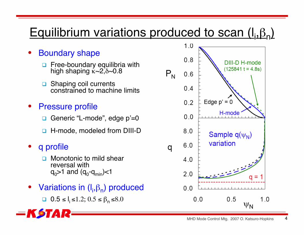
Equilibrium variations produced to scan (li,βn)• Boundary shape

Free-boundary equilibria withhigh shaping κ~2,δ~0.8

Shaping coil currentsconstrained to machine limits

• Pressure profile Generic “L-mode”, edge p’=0 H-mode, modeled from DIII-D

• q profile Monotonic to mild shear

reversal withq0>1 and (q0-qmin)<1

• Variations in (li,βn) produced 0.5 ≤ li ≤1.2; 0.5 ≤ βn ≤8.0


Ideal stability(DCON): conducting wall allows significantpassive stabilization for n=1 H-mode pressure profile

• “inner” wall used• Wall-Stabilized βn is a factor

of two greater then forequilibrium without wall atli ~ 0.7

• Wall-Stabilized βn from DCON agreeswith VALEN-3D value

• “outer” wall used• Wall-Stabilized βn > 6.5 (larger

than the result using “inner” wall at li ~ 0.7)

• Optimistic, but does not agree withVALEN-3D. “Inner” wall is more realisticand should be used in DCON analysis


L-mode pressure profile has largen=1 stabilized region

• “inner” wall used• Wall-Stabilized region

at lowest li (Unfavorablefor n=0 stabilization)

• Possible difficulty toaccess with L-mode confinement.

• n=2 stability has higher no-wall& lower with-wall limits than n=1for H-mode and L-modepressure profile Internal n=2 modes were

observed in NSTX duringn=1 active RWMstabilization.


Conducting hardware, IVCC set up in VALEN-3D*

based on engineering drawings• Conducting structures

modeled Vacuum vessel with

actual port structure Center stack back-

plates Inner and outer

divertor back-plates Passive stabilizer PS Current bridge

• Stabilization currentsdominant in PS 40 times less

resistive than nearbyconductors.

n=1 RWM passive stabilization currents

*Bialek J. et al 2001 Phys. Plasmas 8 2170


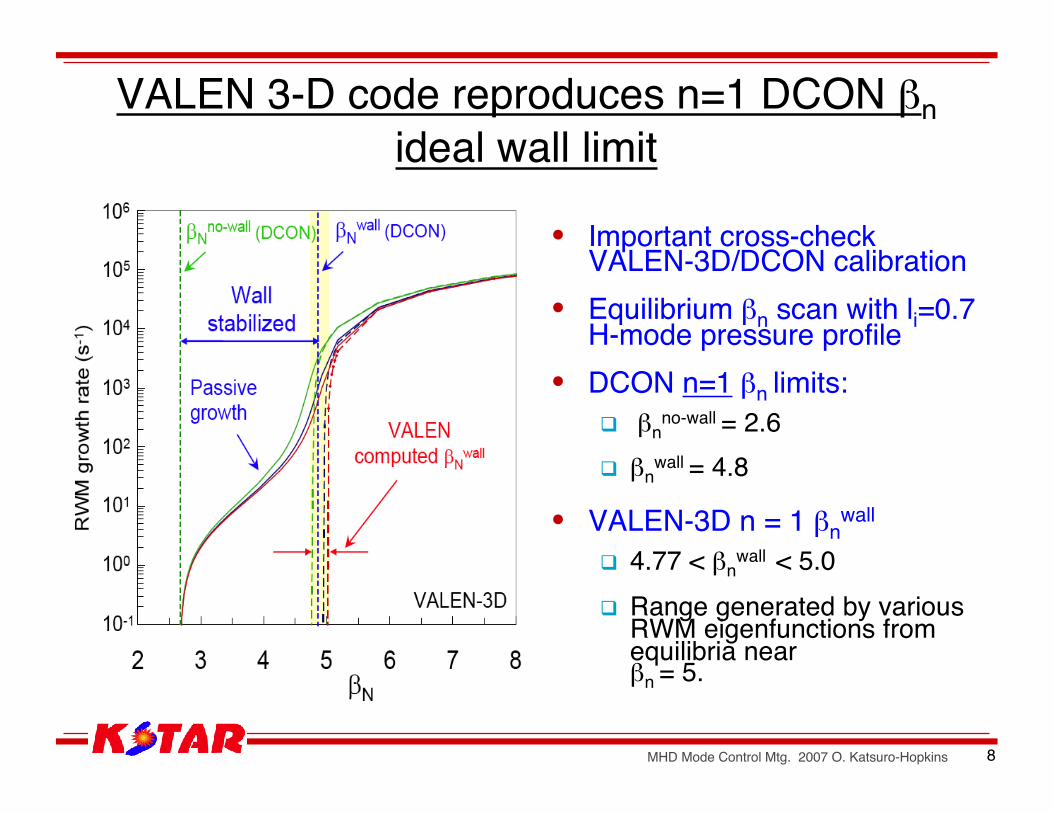
VALEN 3-D code reproduces n=1 DCON βnideal wall limit

• Important cross-checkVALEN-3D/DCON calibration

• Equilibrium βn scan with li=0.7H-mode pressure profile

• DCON n=1 βn limits: βn

no-wall = 2.6 βn

wall = 4.8

• VALEN-3D n = 1 βnwall

4.77 < βnwall < 5.0

Range generated by variousRWM eigenfunctions fromequilibria nearβn = 5.


IVCC allows active n=1 RWM stabilizationnear ideal wall.

• Active n=1 RWMstabilization capability with

Optimal ability for modestabilization

Mid-plane IVCC used

• Equilibrium βn scan withli=0.7 H-mode pressureprofile

• Computed βn limits βn

no-wall = 2.56 βn

wall = 4.76

€

Cβ =βn −βn

no wall

βnwall −βn

no wall > 98%


Power estimates bracket needs for KSTAR RWM control

Unloaded IVCCL=10µHR=0.86mOhmL/R=12.8ms

FAST IVCC circuitL=13µHR=13.2mOhmL/R=1.0ms

Proportional gaincontroller

White noise (1.6-2.0G RMS)

(RMS values)

NSTX 120047 ΔBp sensors

(RMS values)Cβ IIVCC(A) VIVCC(V) PIVCC(W) IIVCC(A) VIVCC(V) PIVCC(W)80% 30 1.6 45 362 0.7 25395% 41 2.0 82 430 0.8 307

80% 20.9 1.56 30.0 1.9e3 24.9 62e395% 28.3 1.78 50.6 9e3 119 1.8e6


Power estimates bracket needs for KSTAR RWM control

• Initial results using advanced Linear Quadratic Gaussian (LQG) controller yieldfactor of 2 power reduction for white noise.

• LQG controller consists of two steps: Balanced Truncation of VALEN state-space for fixed βn Optimal controller and observer design based on the reduced order system

Unloaded IVCCL=10µHR=0.86mOhmL/R=12.8ms

FAST IVCC circuitL=13µHR=13.2mOhmL/R=1.0ms

LQGcontroller

Proportional gaincontroller

White noise (1.6-2.0G RMS)

(RMS values)

NSTX 120047 ΔBp sensors

(RMS values)Cβ IIVCC(A) VIVCC(V) PIVCC(W) IIVCC(A) VIVCC(V) PIVCC(W)

80% 30 / 29 1.6 / 0.8 45 / 24 362 0.7 25395% 41 / 35 2.0 / 0.9 82 / 34 430 0.8 307

80% 20.9 1.56 30.0 1.9e3 24.9 62e395% 28.3 1.78 50.6 9e3 119 1.8e6


State-space control approach may allowsuperior feedback performance

• VALEN circuit equations after including plasma stability effects the fluxes at thewall, feedback coils and plasma are given by

• Equations for system evolution are given by

• In the state-space form

where& measurements are sensor fluxes. State-space dimension ~1000elements!

• Classical control law with proportional gain defined as

€

r Φ w =

t L ww ⋅

r I w +

t L wf ⋅

r I f +

t L wp ⋅ Id

r Φ f =

t L fw ⋅

r I w +

t L ff ⋅

r I f +

t L fp ⋅ Id

Φp =t L pw ⋅

r I w +

t L pf ⋅

r I f +

t L pp ⋅ Id

€

t L ww

t L wf

t L wpt

L fwt

L fft

L fpt L pw

t L pf

t L pp

⋅

ddt

r I wr I fId

=

t R w 0 00

t R f 0

0 0t R d

⋅

r I wr I fId

+

r 0 r V f0

€

r ˙ x =t A

r x +

t B

r u

r y = C

r x

€

r x =

r I w

r I f Id( )

T;

t A = −

t L −1 ⋅

t R ;

t B =

t L −1 ⋅

t I cc;

r u =

r V f

€

r u = −

t G p

r y

€

r y =

r Φ s


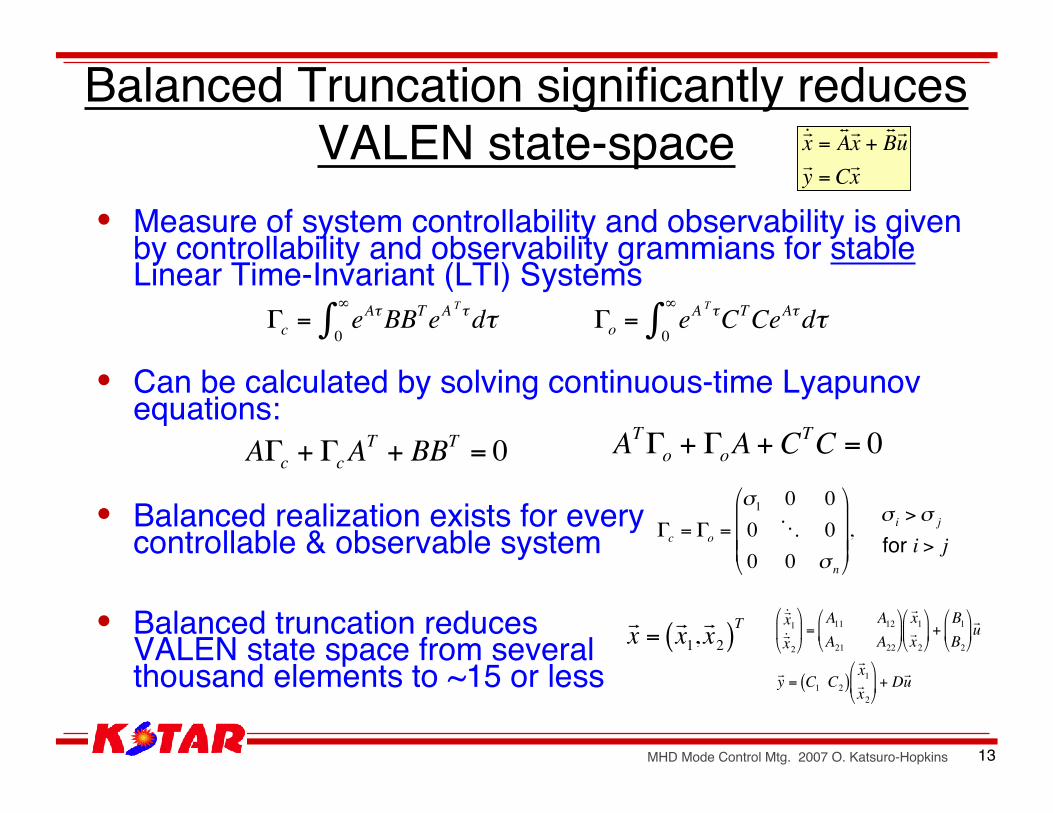
Balanced Truncation significantly reducesVALEN state-space

• Measure of system controllability and observability is givenby controllability and observability grammians for stableLinear Time-Invariant (LTI) Systems

• Can be calculated by solving continuous-time Lyapunovequations:

• Balanced realization exists for everycontrollable & observable system

• Balanced truncation reducesVALEN state space from severalthousand elements to ~15 or less

€

Γc = eAτBBT0

∞

∫ eATτdτ

€

Γo = eATτCTCeAτ

0

∞

∫ dτ

€

AΓc + ΓcAT + BBT = 0

€

ATΓo + ΓoA + CTC = 0

€

Γc = Γo =

σ1 0 00 O 00 0 σ n

,

σ i >σ j

for i > j

€

r ˙ x 1r ˙ x 2

=

A11 A12

A21 A22

r x 1r x 2

+

B1

B2

r u

r y = C1 C2( )

r x 1r x 2

+ D

r u

€

r x =

r x 1,

r x 2( )T

€

r ˙ x =t A

r x +

t B

r u

r y = C

r x


HSV spectrum of KSTAR VALEN state-space suggests areduction of stable part of the system to just 2 balanced states

• LQG controller uses 4 central IVCC & 16 mid-plane poloidal sensors

• Clear gap in HSV spectrum

• Largest SV includes the full system frequency response up to an RWMpassive growth rate.

# of modes

HSV

i

Sing

ular

Val

ues

Frequency rad/sec

___ Full system- - - Reduced system (Nr=3)

€

} Gap ⇒ Nr = 1 RWM + 2


Closed System Equations with Optimal Controller and OptimalObserver based on Reduced Order Model

€

˙ x ˆ ˙ x

=

A −BKcCr

K f C F

xˆ x

+

0K f

ω

F = Ar −K f Cr − (Br −K f Dr )KcCr

€

x = Ax + Buy = Cx +ω

€

ˆ x = Ar ˆ x + Bru + K f (y − ˆ y )ˆ y = Cr ˆ x + Dru

€

u = −Kc ˆ x €

y

€

ˆ x

€

u

€

ωMeasurementnoise

Full order VALENmodel

Optimal observer

Optimal controller

⇐Closed loop continuous systemallows to Test if Optimal controller and observer

stabilizes original full order model Verify robustness with respect to βn

Estimate RMS of steady-state currents,voltages and power


Advanced controller methods planned to be testedon NSTX with future application to KSTAR

• VALEN NSTX Model includes Stabilizer plates for kink

mode stabilization External mid-plane control

coils closely coupled tovacuum vessel

Upper Bp sensors in actuallocations

Compensation of controlfield from sensors

Experimental Equilibriumreconstruction (includingMSE data)

• Present control system onNSTX uses Proportional Gain

RWM active stabilization coils

RWM sensors (Bp)

Stabilizerplates


Advanced control techniques suggests significant feedbackperformance improvement for NSTX up to = 95%

• Classical proportionalfeedback methods VALEN modeling of

feedback systems agreeswith experimental results

RWM was stabilized up toβn = 5.6 in experiment.

• Advanced feedbackcontrol may improvefeedback performance Optimized state-space

controller can stabilize upto Cβ=87% for upper Bpsensors and up to Cβ=95%for mid-plane sensors

Uses only15 modes foroptimal observer andcontroller design 1.E+00

1.E+01

1.E+02

1.E+03

1.E+04

4 4.5 5 5.5 6 6.5 7 7.5

βn

Gro

wth

rate

1/

sec Passive

Ideal Wall

Active Feedback

MC NR=13 Midplanesensors

MC NR=15 s=0.15849Upper Bp sensors

Gro

wth

rate

(1/s

)

βN

DCONno-wall

limit

Experimental (control off)(β collapse) With-wall limit

active controlpassivegrowth

activefeedback

Experimental (control on)

AdvancedFeedback

Bp sensors

AdvancedFeedback

M-P sensors

€

βn βnwall


Next steps and future work on the KSTARstability analysis

• Expand equilibrium / ideal stability analysis as needed Collaborate on equilibrium reconstructions of first

plasmas

• Closer definition of RWM control system circuit byinteraction with KSTAR engineering team

• Improved noise model for KSTAR sensor noise• LQG controller with plasma rotation for KSTAR• LQG controller tests on NSTX with application to KSTAR

RWM control system design• Critical latency testing for KSTAR RWM control


KSTAR is capable of producing long-pulse, high βn stability research

• Machine designed to run high βn plasmas with low li andsignificant plasma shaping capability

• Large wall-stabilized region to kink/ballooning modes withβn/ βn

no-wall = 2 at highest βn predicted for the device Co-directed NBI, passive stabilizers allow kink stabilization

• Active IVCC mode control system provide strong RWMcontrol IVCC design allows active n= 1 RWM stabilization at very

high Cβ> 98%

• Fast IVCC circuit for stabilization is possible at reasonablepower levels


Optimal controller and observer based on reduced orderVALEN model reduce power and achieve higher βn

Minimize Performance Index:

- state and control weighting matrix,Controller gain for the steady-state can be calculated aswhere is solution of the controllerRiccati equation

Minimize error covariance matrixwhere is Kalman Filter gain and is solution of observerRiccati equation

plant and measurement noise covariance matrix.

€

J =r ˆ x '(τ )Qr (τ )r ˆ x (τ ) +

r u '(τ )Rr(τ )r u (τ )( )dτ

t

T

∫ →min

€

Qr,Rr

€

SAr + ArT S - SBrRr

−1BrT S +Qr = 0

€

Kc = R−1BrT S

€

S

€

K f = PC'W −1

€

P

€

ArP + PArT − PCr

TW −1CrP +VT = 0

€

V , W

Controller:

Observer:

€

E (x − ˆ x )(x − ˆ x )T y(τ ),τ ≤ t{ }→min

€

u = −Kc ˆ x

€

ˆ ˙ x = Ar ˆ x + Bru + K f y −Cr ˆ x ( )


Noise on RWM sensors sets control system power• Gaussian white noise

~1.5Gauss RMS, based on noise inDIII-D RWM Bp sensors

Minimum estimate of control powerconsumption

• Perfect response to RWM• No other coherent modes

• Experimental sensor input NSTX Bp sensor during RWM active

stabilization Maximum estimate of control system

power consumption• DC offset from resonant field

amplification; stray field from passiveplate currents

• The ΔB/B0 larger in ST than at higherapsect ratio

modeling of active control on kstar - general atomics · pdf filemodeling of active control on...

Documents