modeling oceanography food web interactions

Oceanography Vol.22, No.1128

Modeling Food Web Interactions in Benthic Deep-Sea Ecosystems

H E R M E S S P E C I A L I S S U E F E AT U R E

B y K A R L I N E S o E TA E R T A N D D I C K V A N o E V E L E N

Benthic filter-feeding community of brachiopods, bivalves, anemones, and sponges at 1600-m water depth in the Whittard Canyon, Northeast Atlantic. Image courtesy NOCS/JC10, 2007

A Practical Guide

This article has been published in O

ceanography, Volume 22, N

umber 1, a quarterly journal of Th

e oceanography Society. ©

2009 by The o

ceanography Society. All rights reserved. Perm

ission is granted to copy this article for use in teaching and research. Republication, systemm

atic reproduction, or collective redistirbution of any portion of this article by photocopy m

achine, reposting, or other means is perm

itted only with the approval of Th

e oceanography Society. Send all correspondence to: info@

tos.org or Th e o

ceanography Society, Po Box 1931, Rockville, M

D 20849-1931, U

SA.

Oceanography March 2009 129

ABSTR ACT. Deep-sea benthic systems are notoriously difficult to sample. Even more than for other benthic systems, many

flows among biological groups cannot be directly measured, and data sets remain incomplete and uncertain. In such cases,

mathematical models are often used to quantify unmeasured biological interactions. Here, we show how to use so-called linear

inverse models (LIMs) to reconstruct material and energy flows through food webs in which the number of measurements

is a fraction of the total number of flows. These models add mass balance, physiological and behavioral constraints, and diet

information to the scarce measurements. We explain how these information sources can be included in LIMs, and how the

resulting models can be subsequently solved. This method is demonstrated by two examples—a very simple three-compartment

food web model, and a simplified benthic carbon food web for Porcupine Abyssal Plain. We conclude by elaborating on recent

developments and prospects.

INTRoDUCTIoNDeep-water sediments are among the largest and most elusive of Earth’s ecosys-tems. Compared to other ecosystems, we know little about the taxonomy, natural history, and trophic linkages among the organisms that inhabit deep-sea sedi-ments. This limitation makes it difficult to predict the impact of human activities on deep ecosystems, but such predictions are greatly needed because human pres-sures on this ecosystem are increasing rapidly (Glover and Smith, 2003).

The interaction of deep-sea benthic ecosystems with and their impact on global-change phenomena are related to two important functions—biogeochem-ical and biological. On the one hand, sediments are sites of organic matter burial, and nutrient regeneration and removal, and thus play an important role in the ocean’s biogeochemical cycles

frameworks have been applied to analyze and understand the processes in sedi-mentary systems (Soetaert et al., 2002). Diagenetic models focus on the role sediments play in the global cycles of essential elements (C, N, P…) and con-sider sediments to be shaped by physical processes and biochemical reactions. In contrast, benthic food web models study the flows of energy or matter between biological functional groups.

There are several good reviews and recent books that deal with diagenetic modeling and its applications (e.g., Burdige, 2006). In contrast, texts on food web modeling are typically case studies with only short introductions to the methodology employed. In this paper, we focus on the latter types of models and give a practical account of their applications and results.

(Sarmiento and Gruber, 2006) and long-term removal of CO2 (Middelburg and Meysman, 2007). On the other hand, processing of organic matter through the food web and resulting secondary production ultimately fuels commer-cially interesting demersal fish com-munities (Graf, 1992).

The potential significance of deep-sea regions has directed considerable scientific and technological effort to better understanding of both functions of this remote environment. Although the information gathered through these efforts has markedly enhanced our knowledge of the deep-water benthos, most of the research is reductionist in nature, investigating isolated parts of the ecosystem. Mathematical models can merge this fragmentary information into a realistic integrative framework.

At least two different theoretical


BENTHIC FooD WEBSWith the exception of hydrothermal vent and cold seep environments, which are driven by chemosynthetic energy, deep-sea benthic systems ultimately depend on an allochtonous food sup-ply in the form of detritus derived from primary production in the euphotic zone (Figure 1). Before detritus becomes incorporated into the sediment, part of the food is consumed by suspension feeders that filter organic matter from the water mass overlying the bottom (Gage and Tyler, 1991) or by sediment-dwelling deposit-feeders (Blair et al., 1996; Drazen et al., 1998). The remain-der of the food is ingested by sediment-inhabiting detritivores of various sizes (e.g. Graf, 1992) and by bacteria (Lochte and Turley, 1988) that respond rapidly to the supply of particulate organic matter in terms of increased metabolic activity (Witte et al., 2003; Moodley et al., 2005) or growth and reproduction (Tyler et al., 1982; C.R. Smith et al., 2008; K.L. Smith et al., 2008). The detritivores are con-sumed by predators, which may them-selves be preyed upon by larger animals such as fish. The waste products of all consumers become food for detritivores and bacteria (detritus) or are exchanged with the water column (CO2, nutrients).

The flows of food to the primary benthic consumers and the recycling of matter from one biotic component to

another comprise the benthic food web. How benthic communities process the primary material and convert organic matter as it passes through each trophic link has significant consequences for ecosystem properties, such as food web stability (e.g., Rooney et al., 2006), and for linking benthic secondary produc-tion with higher trophic levels that are eventually harvestable by humans (Pauly et al., 1998). In addition, food web structure and functioning affects biogeochemical properties such as carbon sequestration (Middelburg and Meysman, 2007), carbon turnover (Meysman and Bruers, 2007), and nutri-ent regeneration (Vanni, 2002). Thus,

the identification and quantification of energy pathways through the major ecosystem components is a basic element of food web studies. The ultimate goal is to achieve a quantitative understanding of the functional interactions between biological components in order to even-tually predict the response of deep-water systems to global change phenomena.

Quantification of biological interac-tions in terms of carbon or organic matter flows is strongly hampered by the lack of sufficient high-quality empiri-cal data (Brown, 2003). This is because the elucidation of food web flows from direct measurement or experimenta-tion is notoriously difficult, even for

Karline Soetaert (k.soetaert@nioo.

knaw.nl) is Senior Researcher, Center for

Estuarine and Marine Ecology, Netherlands

Institute of Ecology (NIOO-KNAW), Yerseke,

The Netherlands. Dick van Oevelen

is Postdoctoral Researcher, Center

for Estuarine and Marine Ecology,

NIOO-KNAW, Yerseke, The Netherlands.

CO2

phytoplankton

zooplankton

suspension and epibenthic feeders

bacteria

(phyto)detritus meiobenthos

deposit feeders

predators

burial

102 - 10

3 m10

-2 - 100 m

CO2

Figure 1. Scheme of a simplified deep-sea benthic food web.


comparatively well-studied shallow-water benthic systems (e.g., van Oevelen et al., 2006a,b). The inaccessibility of deep-sea ecosystems adds an extra level of complexity, rendering deep-water data sets archetypical examples of undersam-pled food webs. Most deep-water data sets consist of biomass estimates of large functional groups and an occasional rate measurement only. Given the complexity of food webs, the knowledge based on field measurements alone is insufficient to derive a coherent picture of carbon flows in these systems.

To overcome these data limitations and extract as much information from them as possible, so-called linear inverse models (LIM) have been developed. The linear inverse modeling methodology allows quantifying biological interac-tions in a complex food web from an incomplete and uncertain data set. In what follows, we first explain how linear inverse models are developed and solved, and then we elaborate on recent devel-opments and prospects.

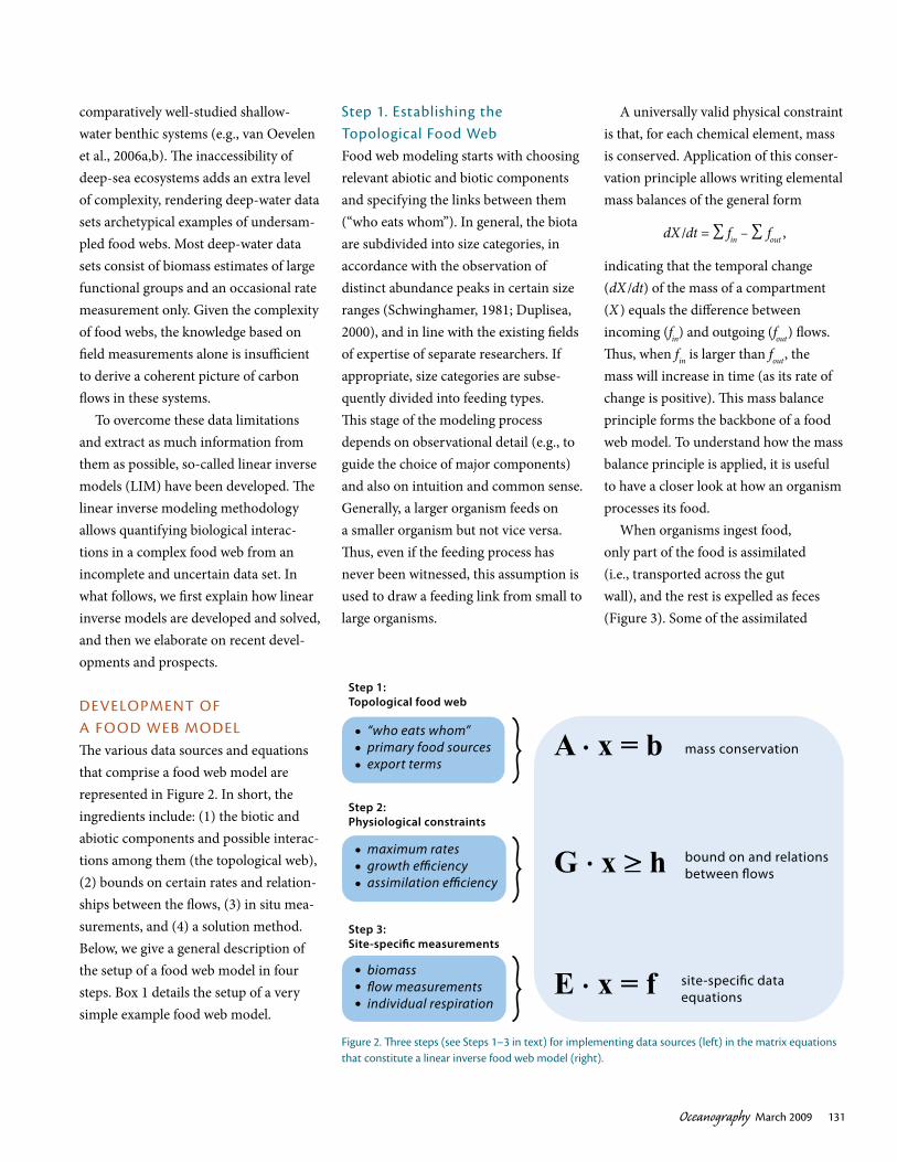
DEVELoPMENT oF A FooD WEB MoDELThe various data sources and equations that comprise a food web model are represented in Figure 2. In short, the ingredients include: (1) the biotic and abiotic components and possible interac-tions among them (the topological web), (2) bounds on certain rates and relation-ships between the flows, (3) in situ mea-surements, and (4) a solution method. Below, we give a general description of the setup of a food web model in four steps. Box 1 details the setup of a very simple example food web model.

Step 1. Establishing the Topological Food WebFood web modeling starts with choosing relevant abiotic and biotic components and specifying the links between them (“who eats whom”). In general, the biota are subdivided into size categories, in accordance with the observation of distinct abundance peaks in certain size ranges (Schwinghamer, 1981; Duplisea, 2000), and in line with the existing fields of expertise of separate researchers. If appropriate, size categories are subse-quently divided into feeding types.This stage of the modeling process depends on observational detail (e.g., to guide the choice of major components) and also on intuition and common sense. Generally, a larger organism feeds on a smaller organism but not vice versa. Thus, even if the feeding process has never been witnessed, this assumption is used to draw a feeding link from small to large organisms.

A universally valid physical constraint is that, for each chemical element, mass is conserved. Application of this conser-vation principle allows writing elemental mass balances of the general form

dX /dt = ∑ fin – ∑ fout ,

indicating that the temporal change (dX /dt) of the mass of a compartment (X) equals the difference between incoming (fin) and outgoing (fout) flows. Thus, when fin is larger than fout, the mass will increase in time (as its rate of change is positive). This mass balance principle forms the backbone of a food web model. To understand how the mass balance principle is applied, it is useful to have a closer look at how an organism processes its food.

When organisms ingest food, only part of the food is assimilated (i.e., transported across the gut wall), and the rest is expelled as feces (Figure 3). Some of the assimilated

mass conservation

bound on and relations between flows

site-specific data equations

“who eats whom”primary food sourcesexport terms

maximum ratesgrowth efficiencyassimilation efficiency

biomassflow measurementsindividual respiration

Step 1: Topological food web

Step 2: Physiological constraints

Step 3:Site-specific measurements

A x = b .

G x > h .

E x = f .

Figure 2. Three steps (see Steps 1–3 in text) for implementing data sources (left) in the matrix equations that constitute a linear inverse food web model (right).


Consider a very simple food web model comprised of three components (in the figure at right): Blue boxes represent (1) detritus, (2) bacteria growing on detritus, and (3) fauna grazing on bacteria. The system is driven by an external import of detritus (f0). There are two consumption flows (f1 and f2), one feces production flow (f3), and two respiration flows (f4 and f5); demersal fish graze on the fauna (f6). Neither Co2 (the respira-tion product) nor the fish are modeled explicitly as food web compart-ments; rather, they are considered external compartments. The three mass balance equations relate the rate of each compart-ment’s change to the seven source and sink flows. If we assume that the compartments are invariant in time, they can be written as

dDetritus = 0 = f0 – f1 – f3dt

dBacteria = 0 = f1 – f2 – f4dt

dFauna = 0 = f2 – f3 – f5 – f6dt

These equations can be written in a more general way as:

0 = 1 • f0 – 1 • f1 + 0 • f2 + 1 • f3 + 0 • f4 + 0 • f5 + 0 • f6

0 = 0 • f0 + 1 • f1 – 1 • f2 + 0 • f3 – 1 • f4 + 0 • f5 + 0 • f6

0 = 0 • f0 + 0 • f1 + 1 • f2 – 1 • f3 + 0 • f4 – 1 • f5 – 1 • f6

to relate the rate of change (left-hand side, assumed 0) to a sum of prod-ucts, where each product is composed of the flow times a coefficient. It is convenient to collect these coefficients in a matrix, leading to the following notation:

0 =

1 −1 0 1 0 0 0

0 1 −1 0 −1 0 0

0 0 1 −1 0 −1 −1

•

f0

f1

f2

f3

f4

f5

f6

orwritten with x=[ f0… f6] as A • x = 0.

The positivity of the flows is written as

x ≥ 0.

Physiological considerations (Step 2 in Figure 2) are implemented through the inequality constraints. For example, bacterial carbon is high quality food for benthic fauna; therefore, a reasonable assumption is that feces production (f3) is small, between 10% and 30% of faunal ingestion (f2). This gives the following two inequalities:

f3 ≥ 0.1 • f2f3 ≤ 0.3 • f2

0 0 −0.1 1 0 0 0

0 0 0.3 −1 0 0 0

• x ≥

0

0

or .

Growth respiration is assumed to be between 20% and 40% of assimi-lated detritus (bacteria) or assimilated bacteria (fauna):

and .f4 ≥ 0.2 • f1

f4 ≤ 0.4 • f1

f5 ≥ 0.2 • ( f2 − f3)

f5 ≤ 0.4 • ( f2 − f3)

Site-specific flow measurements can be directly included. Suppose that detritus deposition has been measured with sediment traps at f0 = 1 g C m-2 yr-1. This measurement gives the following equation:

1 0 0 0 0 0 • x = 1 .

Box 1. Setting up a Simplified Food Web

FaunaBacteria

Detritus

FaunaBacteria

Detritus

FaunaBacteria

Detritus

FaunaBacteria

Detritus

f0 f6

f3f1

f4 f5

f2


fraction of the food is used as building blocks for growth and reproduction (sec-ondary production), and some of it is oxidized to provide the energy required to maintain basal metabolism, form new biomass, reproduce, and move. For het-erotrophic organisms, the energy needed for growth and for maintenance is paid by respiration, that is, the oxidation of simple organic compounds, while other, so-called chemo-autotrophic organisms produce biomass from chemical energy and inorganic compounds. From the modeler’s point of view, the functioning of an organism is analogous to a chemi-cal “factory” that uses raw materials

(food) to produce valuable goods (bio-mass), while consuming energy (respira-tion) and producing waste (feces) in the production process (Figure 3).

The principle of mass conservation states that, if the organism is not pre-dated upon, then the ingested food is either respired, defecated, or will serve biomass increase because of growth (Figure 3). We write this as

Growth = dC /dt = ingestion – predation mortality – defecation – respiration,

where C is the biomass of the organism, and dC /dt is its growth (i.e., the rate at which this biomass changes in time).

This so-called mass-balance equation equates biomass changes to feeding flows minus loss terms (respiration, feces production, mortality).

The mass balances of all food web components are intimately linked: if spe-cies A feeds on species B, not only will there be a flow of biomass from B to A, but also a loss of similar magnitude from species B. In addition, feces will be produced, inducing a flow from B to detritus. The coupled set of mass balance for several functional groups considered together forms the backbone of the food web model.

If a flux from functional group i to

bacteria

meiobenthos

deposit feeders

predators

The factory analogue

ingestion production

defecation

The organism level

f3

f2f1 f6 f7

f4

f5

(phyto)detritus

The mass balance

dB dt

= f1 + f2 + f3 - f4 - f5 - f6 - f7

ingestion defection predation basal respiration

growth respiration

respiration

Figure 3. The mass balance of one organism from the food web (left) and the factory analogue (right).


functional group j is denoted as dCidt

Fj → i –= Fi → j – Fecesi – Respi.∑n

j = 1∑n

j = 1,

then the mass balance for a biotic food web component (i = 1,..n) is given by

dCidt


j = 1∑n

j = 1

This equation can be made more com-pact by denoting detritus as component “0” and carbon dioxide as component -1, so that we obtain

dCidt

Fj → i –= Fi → j i = 0,..n.∑n

j = 0∑n

j = –1

In food web models, the flows dCidt


j = 1∑n

j = 1 and dCidt


j = 1∑n

j = 1 are the unknowns (x) to be quanti-fied. The mass-balance equations are just sums and subtractions of these unknown quantities. These linear equations are conveniently cast into matrix notation as

A • x = b (1)

in which x is a vector with the unknown flows, and b is a vector with the rates of change of the components.

Because flows have a direction (i.e., they are non-negative quantities), the following inequalities also hold:

x ≥ 0. (2)

Step 2. Physiological and Behavioral ConstraintsThe physiology and behavior of organ-isms imposes lower and upper limits on their feeding and growth rates. When organisms search for food, the encounter

rate and external handling time deter-mines maximal foraging capacity (Holling, 1966). The ingested food is hydrolyzed and assimilated, but these processes are limited by physiologi-cal and digestive constraints (Jumars, 2000). Consequently, animals can only process a finite amount of food per unit of time (i.e., there are upper bounds on weight-specific ingestion rates). Often, these maximal weight-specific rates scale inversely with organism size (Peters, 1983). When combined with biomass estimates (see below), these maximum rates impose an upper bound on grazing flows, providing important constraints on the magnitudes of the ingestion flows in the food web model.

Similar allometric rules (allometry is the study of the relative growth of a part of an organism in relation to the growth of the whole) apply for respiration flows (e.g., Mahaut et al., 1995), although it is customary here to impose respiration rates as lower bounds (i.e., a minimal basal respiration required to ensure basic metabolic integrity of the organism).

Other physiological considerations impose relationships between flows. The production of biomass and/or reproduc-tive tissue costs energy. As a simplifica-tion, it can be assumed that these costs are paid by respiring part of the ingested food, and hence the feeding and respi-ration flows are directly related. This

relationship is determined by the amount of energy required to build a specific amount of biomass (recall the factory analogue in Figure 3, where respiration delivers the energy to produce a certain amount of goods). Classically, this is rep-resented by growth efficiency—the ratio of secondary production (growth) to assimilated food, which is generally on the order of 60–70% (Calow, 1977) and at most 80% (Schroeder, 1981).

In addition, there is a similar relation-ship between feeding and defecation: organisms cannot produce more feces than the amount of food they ingest, but they have to assimilate a certain fraction to balance the loss terms. Depending on the quality of the food, a small or large fraction of it will be expelled as feces (Calow, 1977; Schroeder, 1981). Most often, this dependency is expressed by the so-called assimilation efficiency—the ratio of assimilated food (the food that is not defecated) to ingested food (Conover, 1966), which is roughly on the order of 20%, 60%, and 80% for detritivores, herbivores, and carnivores, respectively (Hendriks, 1999). Rather than assuming that growth and assimila-tion efficiencies are exactly known, it is more realistic to impose upper and lower bounds on these efficiencies.

The constraints on ingestion rates mentioned above as well as growth and assimilation efficiency put bounds

ALTHoUGH THE INFoRMATIoN GATHERED THRoUGH ENVIRoNMENTAL STUDIES HAS MARKEDLy ENHANCED oUR KNoWLEDGE oF THE DEEP-WATER BENTHoS, MoST oF THE RESEARCH IS REDUCTIoNIST IN NATURE, INVESTIGATING ISoLATED PARTS oF THE ECoSySTEM. MATHEMATICAL MoDELS CAN MERGE THIS FRAGMENTARy INFoR-MATIoN INTo A REALISTIC INTEGRATIVE FRAMEWoRK.

“”


on various flows and on relationships between flows. These constraints can also be cast in a matrix equation, comprising inequality conditions:

G • x ≥ h. (3)

Step 3. In Situ MeasurementsThe data types mentioned above make use of general biological principles that apply to most ecosystems. To tailor the model to a food web of a specific loca-tion, in situ measurements are indis-pensable. These specific data are of great importance: without them, the model would make the fairly unrealistic predic-tion that the food web is exactly the same at every place on Earth! Fortunately, many different data types that are col-lected by deep-sea ecologists can be directly used.

For instance, biomasses of organisms when multiplied with estimated minimal or maximal weight-specific rates (see above) provide important bounds on respiration and feeding flows.

Some food web flows can be measured directly, such as the respiration rate of a single biotic component, food con-sumption rates (e.g., of deep-sea fishes; Bulman and Koslow, 1992), and bacterial mortality (e.g., induced by viral lysis; Mei and Danovaro, 2004; Danovaro et al., 2008). Such flow measurements can be directly added to the food web model.

Other in situ rate measurements may represent simple combinations of mul-tiple flows in the food web. For instance, bacterial production is the net effect of bacterial uptake of dissolved organic car-bon (DOC) minus bacterial respiration; the influx of oxygen across the sediment-water interface is the summed respira-tion of all the food web components.

Finally, the diet composition of a

grazer imposes relationships among the different ingestion flows of the grazer. To quantify these relationships requires information on the importance of certain diet constituents with respect to one another. Diet information can come from gut analysis of large animals (e.g., for deep-sea fishes), or from the use of biomarkers, such as stable isotopes of nitrogen (δ15N) and carbon (δ13C) (Vander Zanden and Rasmussen, 1999; Iken et al., 2001; Polunin et al., 2001) or fatty acids (Howell et al., 2003). Stable isotope values from different food sources mix proportionally in the con-sumer, and such a mixing formulation fits seamlessly in food web linear inverse models (Van Oevelen et al., 2006b,c; Eldridge et al., 2005). Similarly, deriving diet information from fatty acid com-positions relies on the same assumption (Iverson et al., 2004).

Important data can also come from ecological stoichiometry, in which food web interactions are constrained because empirical data in one currency (e.g., C) are coupled to data in another currency (e.g., N, P, or O2) (e.g., Vézina and Platt, 1988; Jackson and Eldridge, 1992; Gaedke et al., 2002).

Because of the valuable information contained in site-specific measurements, the available in situ measurements are generally adopted as they are (i.e., with-out uncertainty) and implemented as equality equations, which can be written in a matrix form that is identical to the mass balance equation

E • x = f. (4)

Step 4. Model SolutionThe measurement and compilation of the data in Steps 1–3 depends on the expertise of the field and experimental

biologist. It is only in the last step that the mathematically inclined personality, the modeler, comes in. This person puts all of the acquired information into a mathematical framework to find a solu-tion to the mathematical model.

The entire model, consisting of mass balance equations and positivity constraints (Step 1), physiological con-straints (Step 2), and in situ data (Step 3), is combined in Step 4 using appallingly simple, linear equations (equations 1–4). In Box 1, we show how to compose these equations for a very simple food web.

The solution to this model is a set of flow values (x) that is consistent with the four sets of equations. Depending on the number of equations relative to the number of unknowns, different methods of solution are used. These model solution methods bear a strong resemblance to linear regression and are intimately linked to the determi-nacy state of the model (this concept is explained in Box 2).

Ideally, the equations lead to only one solution that perfectly fits the data, called the even-determinacy state (Box 2). This state is achieved when the number of equations is equal to the number of unknown flows (and the equations are internally consistent). Alas, it is very unlikely that, by mere coincidence, the number of equations and unknowns will match; in general, there are too few equations, and there is no unique solu-tion to the model. Thus, some modelers add data from the literature to the site-specific observations to reach the state of even-determinacy. This practice is common in many ECOPATH applica-tions, one of the most-used frameworks for linear inverse modeling (Christensen and Pauly, 1992). However, it is doubtful


whether such artificial inflation of the site-specific data set with data from other locations can be justified.

The most commonly encountered situation is the under-determinacy state—the number of equations is less than the number of unknowns (Box 2), and there is no unique solution that perfectly fits the data. There are two pos-sible outcomes when trying to solve such under-determined models.

First, if some data are “in conflict” with other data, the model is unsolvable and no solution exists that fits all data simultaneously. This situation would be the case when the measured total input of organic matter is insufficient to meet the minimum respiration requirements

(e.g., estimated from physiological con-siderations) of the benthic community (e.g., Smith et al., 2001). This result (albeit undesirable) is important, as it shows that data that seem plausible when evaluated individually may be incon-sistent when viewed in the perspective of the entire food web. Therefore, this outcome may prompt reconsideration of the reliability of the data and/or the food web model.

In contrast, when the data in the under-determined model are internally consistent, there exists an infinite num-ber of valid solutions. In this case, the linear equations define an “ensemble” of plausible webs—a multidimensional solution space containing food web

configurations that do not violate the equations (Figure 4). From this solution space, modelers either extract one set of food web flows, or try to quantify the uncertainty, for example, via the ranges or probability density functions of all flows (see below).

Early modeling studies usually selected one food web from the infinite number of solutions. The principle of parsimony has often been applied as selection criterion (Vézina and Platt, 1988), which implies that the solution for which the sum of squared flows is minimal is selected (Figure 4a). Whereas the parsimony principle provides fairly robust estimates of the food web struc-ture (Vézina and Pahlow, 2003; Vézina

Solving a linear food web model requires finding values for flows (x) that are consistent with the four matrix equations comprising the model (see Box 1). Depending on the determinacy state of the model, it is solved using different methods. The determinacy state is evaluated using the dimensions of the matrices Ax = b and Ex = f. These dimensions are the number of independent equations (rows in A + rows in E) and the number of unknown flows (elements in vector x). The determinacy state can be under-determined if there are fewer equations than unknowns, even-determined if the number of equations and unknowns is equal, or over-determined if there are more equations than unknowns. The solution procedure is very similar to fitting a straight line through data points, and it is instructive to discuss this familiar analogy. A straight line is characterized by two unknown parameters: the slope and intercept. These parameters are quantified by fitting to a data set so that the data are optimally reproduced. With one observation and two unknown parameters, the model is under-determined, and there are infinite numbers of different straight lines that all exactly pass through that single data point (A in the figure at left). Similarly, under-determined food web models will have an infinite number of solutions. With two data points, the model is even-determined, as there are also two parameter values to derive. only one straight line passes exactly through two points. Similarly, even-determined food webs will have one unique solu-tion (B in the figure at left). The over-determined state is encountered when there are more data points than unknowns. Not all data points can be exactly reproduced due to unavoidable measurement error, but a unique parameter combination repro-duces the data optimally (C in the figure at left).

Box 2. Determining the Determinacy State of a Model

X

A

B

C

Y


et al., 2004), it has often been criticized because it lacks a sound ecological justification (Niquil et al., 1998; Kones et al., 2006). Moreover, the parsimoni-ous web often takes extreme values (i.e., it lies at the boundaries of the solu-tion space) (Diffendorfer et al., 2001; Kones et al., 2006).

Alternatively, the uncertainty of flow values can be explored, for example, by estimating the range (min-max) of all flow values (Figure 4b; see Klepper and Van de Kamer, 1987; Van Oevelen et al., 2006c). More recently, a method has been developed in which mean values and standard deviations of the flow values are calculated from a representa-tive set of solutions that were sampled

via Monte Carlo methods (Figure 4; see Kones et al., 2006).

As there is not much to be gained by investing in additional data on flows that are already well constrained, the estimation of flow uncertainty provides essential information about which flows need to be measured preferentially. Note that it may be difficult to ascertain the most critical knowledge gaps in the data without the use of a model. Thus, measurements and modeling are complementary: field data act as input for reducing model uncertainty, while models may be used to improve the cost-effectiveness of field campaigns by pinpointing the essential measurements that should be acquired.

BENTHIC FooD WEBS IN HERMESWithin the HERMES project, food web reconstructions are prepared or have been created for Nazaré Canyon, a Rockall Bank cold-water coral com-munity, an Arctic food web in Fram Strait (Hausgarten observatory of the Alfred Wegener Institute for Polar and Marine Research), and several open slope food webs in the western and central Mediterranean. In addition, a modeling study on the complete food web of the Porcupine Abyssal Plain is in preparation and will include data from the isotope labeling experiment using an addition of fresh algal carbon to the sediment from Witte et al. (2003). A simplified benthic carbon food web for this system is presented in Box 3 and Figures 5 and 6.

x 1

x 2

x 3

x 1

x 2

x 3 B A C - > M A C

M A C - > D E T

B A C - > C O 2

x 1

x 2

x 3

Ensemble of solutions

Parsimonious solution Range estimation Bayesian sampling

selects one solution estimate of flow range flow distribution in ensemble

Figure 4. Solution methods for an under-determined food web model. There exists an ensemble of food webs that are all equally likely (upper). Either one food web is taken from this ensemble (lower left), or the ranges of food webs are estimated (lower middle), or a representa-tive sample of the ensemble is taken (lower right).


The Porcupine Abyssal Plain (Northeast Atlantic), located at ~ 4850 m depth, is one of the best-studied deep-sea sites. Here we give a simpli-fied model of this ecosystem (Figures 5 and 6). A more elaborate model is under construction. Detritus from the water column (det_w) adds to the sedimentary detritus compartment (det), where it is taken up directly by nematodes (nem) and macrobenthos (mac), and dissolves to become dissolved organic carbon (doc). Part of the dissolved organic carbon is taken up by bacteria (bac), and the other part effluxes to the water column (doc_w). Bacteria in turn are grazed upon by nematodes and macrobenthos or may lyse (e.g., by viruses). Respiration by the biotic compartments induces a flux to the dissolved inorganic carbon pool in the water column (dic_w). Nematodes and macrobenthos produce feces that add to the detritus compartment. Nematodes are preyed upon by macrobenthos. Finally, nematodes and macrobenthos are preyed upon by megabenthic predators, but because they are not considered

in this model, these grazing fluxes are described as export fluxes from the food web. Site-specific data on stock sizes of the biotic and abiotic compartments and process rates from the literature (Tables 1 and 2) are combined with generic physiological constraints (Van oevelen et al., 2006c) (Table 3) and added to the model. The implemented data are internally consistent, and the model is solved (Figure 6) by estimating the parsimonious (simplest) solution, the Monte Carlo solution, and the associated flow ranges (Figure 6A) (see Figure 4 for conceptual visualization). overall, the flow ranges are relatively small, indicating that, notwithstanding the limited amount of data, the flows in the food web are well constrained. However, some flows (e.g., det → nem and nem → det) are highly uncertain (Figure 5), and strongly positively cor-related (Figure 6). This result indicates that it is possible to quantify the net flux from detritus to nematodes, but not the separate flows.

Table 1. Data on carbon stocks used for the Porcupine Abyssal Plain case study. Data are for the upper

5 cm of the sediment and expressed in mgC m-2.

Compartment Stock Reference

Detritus 28654* Danovaro et al., 2001

Dissolved organic carbon 234 Ståhl et al., 2004

Bacteria 1695 Pfannkuche and Soltwedel, 1998

Nematodes 5 Witte et al., 2003

Macrobenthos 157 Flach et al., 2002

* Sum of biopolymeric (i.e., fatty acids, amino acids, and carbohydrates) carbon equivalents.

Table 2. Data on fluxes used for the Porcupine Abyssal Plain case study. Process rates are in mgC m-2 d-1. The expression in flows indicates which flow (or sum of flows) should equate to the measured process rate.

Process Expression in Flows Value Reference

Efflux of dissolved organic carbon doc → doc_w 0.83 Lahajnar et al., 2005

Sediment community respiration bac → dic + nem → dic + mac → dic 5.43 Witbaard et al., 2000

Box 3. The Benthic Food Web at Porcupine Abyssal Plain


Table 3. Generic physiological constraints used in the Porcupine Abyssal Plain case study. A flow is designated as (source → sink) and standings stocks (Table 1) are designated with compartmentss.

Process Expression in Flows Min Max

Bacterial growth efficiency (–) 1

(doc → bac) – (bac → dic)(doc → bac)

= 0.06 0.32

Detritus degradation rate (d-1) 2

(det → doc) + (det → nem) + (det → mac)detss

= 0.00025 0.016

Assimilation efficiency: nematodes (–) 3

(det → nem) + (bac → nem) – (nem → det)(det → nem) + (bac → nem)

= 0.06 0.30

Net growth efficiency: nematodes (–) 3

[(det → nem) + (bac → nem)] – (nem → det) – [(nem → dic) – nemMR](det → nem) + (bac → nem) – (nem → det)

=

with: nemGR = (nem → dic) – nemMRnemMR = Tlim • 0.01 • nemss

Tlim = Q10 • exp((T-20)/10) = 0.35, with Q10 = 2 and T = 2.5

0.60 0.90

Growth rate: nematodes (d-1) 3

[(det → nem) + (bac → nem)] – (nem → det) – nemGRnemss

= Tlim • 0.05 Tlim • 0.40

Assimilation efficiency: macrobenthos (–) 3

[(det → mac) + (bac → mac) + (nem → mac)] – (mac → det)(det → mac) + (bac → mac) + (nem → mac)

= 0.40 0.75

Net growth efficiency: macrobenthos (–) 3

[(det → mac) + (bac → mac) + (nem → mac)] – mac → det – [mac → dic – macMR][(det → mac) + (bac → mac) + (nem → mac)] – mac → det

=

with:macGR = mac → dic – macMRmacMR = Tlim • 0.01 • macss

0.50 0.70

Growth rate: macrobenthos (d-1)

[(det → mac) + (bac → mac) + (nem → mac)] – (mac → det) – macGRmacss

= Tlim • 0.01 Tlim • 0.05

1del Giorgio and Cole, 1998; 2Henrichs and Doyle, 1986; and 3Van oevelen et al., 2006c


RECENT DEVELoPMENTS AND PRoSPECTSRecent developments in solving linear inverse models tend towards quantifica-tion of residual uncertainty rather than selecting one solution (Kones et al., 2006; Kones et al., 2009). Some research is also directed toward finding a stronger selec-tion criterion rooted in ecological theory, for example, maximizing ascendancy, or maximizing growth (Vézina and Pahlow, 2003; Vézina et al., 2004).

The most important progress will, however, be achieved by the inclusion of better, novel, and different data into

the food web model. As more and dif-ferent types of in situ information are acquired and implemented, the model’s solution space narrows until the flow uncertainties are deemed to be within acceptable ranges.

Currently, most data in inverse food web models are either biomasses or mea-sures of total carbon cycling (e.g., total community respiration or carbon deposition). Information on cycling rates among components in the food web is much more difficult to obtain and therefore much scarcer. Stable isotopic data have provided valuable information

on deep-sea food webs (e.g., Iken et al., 2001; Van Gaever et al., 2006), and for intertidal areas these have proven to be ideal data sources to further constrain the magnitude of carbon flows (Van Oevelen et al., 2006c). However, to be applicable, different food sources should have different signatures and—more importantly—the signatures of food sources should be measurable. The most important challenge will be to increase our ability to distinguish among the dif-ferent sources on which animals actually feed. The (phyto)detritus deposited on the seafloor mixes with the sedimentary

det−>doc

det−>nem

det−>mac

doc−>bac

bac−>doc

bac−>nem

bac−>mac

nem−>det

nem−>mac

mac−>det

det

doc

bac

nem

mac

det_w doc_w dic_w

exp

det

doc

bac

nem

mac

Figure 5. (Upper right) Schematic food web of the (simplified) Porcupine Abyssal Plain model. det_w is detritus in the water column, det is

detritus in the sediment, doc is dissolved organic carbon, bac is bacteria, nem is nematodes, mac is macrobenthos, dic_w is

dissolved inorganic carbon in the water column, doc_w is dissolved organic carbon in the water column, and exp

is export (e.g., predation by megabenthos). Internal flows are black; exchange with external is grey.

(Lower left) The pair-wise set of solutions obtained by the Monte Carlo sampling

method (for internal flows only); each dot is a valid flow value. The histo-

gram on the diagonal represents the distribution of flow

values in the sampled set of solutions.


pool, such that sediment detritus con-stitutes a complex mixture of organic matter with different origins, composi-tion, age, and reactivity (Middelburg, 1989; Middelburg and Meysman, 2007). Certain organisms select only specific fractions of this detritus, so that the stable isotope signature or fatty acid composition of their food may not be simply quantified.

A way around this problem is to manipulate the isotope signature of a food source. For example, when iso-topically labeled algae are amended to in situ or onboard incubation cores,

the organisms that feed on this food will incorporate the elevated isotope signal. The timing and magnitude of isotope enrichment in the consumer provides information on the importance of this food in the consumer’s diet. Notwithstanding the difficulty of car-rying out such replicated experiments in the deep sea, an increasing amount of work that focuses on the transfer of fresh phytodetritus into benthic deep-sea food webs is performed in these environments (e.g., Blair et al., 1996; Moodley et al., 2002; Aberle and Witte, 2003; Witte et al., 2003; Moodley et al.,

2005; Nomaki et al., 2005). In principle, it is also possible to trace the bacterial pathway by isotope enrichment of the dissolved organic carbon pool in the sediment or amending enriched cultured bacteria into sediment cores. Although this method has so far only been applied in intertidal mudflats (Carman, 1990; Van Oevelen et al., 2006a,b; Pascal et al., 2008), only technical difficulties ham-per application of this methodology to deep-sea sediments.

Because the transient data of such isotope tracer experiments cannot be directly entered into the linear equations of the food web model, the solution of the food web model (i.e., the quantified food web flows) needs to be translated into rate constants for each flow. These rates govern dynamic equations that allow simulation of the transfer of the isotope tracer through the food web. Comparing the model simulation results to the data then allows us to select the most likely food web (e.g., Van Oevelen et al., 2006c). A model that couples a lin-ear inverse model with the enrichment experiments performed by Witte et al. (2003) at the Porcupine Abyssal Plain is under construction.

CoNCLUSIoNInverse modeling is a tool that inte-grates scattered information on carbon cycling, diet, stable isotope signatures, and organic matter processing. Such integration will lead to better insight into the structure and functioning of deep-sea food webs, which is much needed because empirical data on deep-sea eco-systems is expensive to gather. Although inverse modeling quantifies a snapshot of the magnitude of food web flows, it is also possible to analyze temporal and/or

●

●

●

●

●

●

●

●

●

●

●

●

●

●

●

●

●

0 5 10 15 20Flow value (mg C/m2/d)

● ParsimoniousMonte Carlo averageRange

Porcupine Abyssal Plain food web

mac → exp

mac → det

mac → dic

nem → exp

nem → mac

nem → det

nem → dic

bac → mac

bac → nem

bac → doc

bac → dic

doc → bac

doc → doc_w

det → mac

det → nem

det → doc

det_w → det

Figure 6. Plot with the parsimonious (simplest)-averaged and Monte Carlo-averaged solutions encompassed by the range for each flow.


spatial dynamics of the food web struc-ture. For example, Donali et al. (1999) reconstructed pelagic food web struc-tures in spring, summer, and autumn to identify temporal dynamics. However, the inverse modeling formalism is not easily used for prediction, because the model does not include the mechanisms that shape food web flows. Nevertheless, if food web quantification is repeated frequently enough and for different sites, certain patterns may emerge that provide clues to the factors that shape the deep-sea food webs. Based on these results, it may then become possible to quantify truly kinetic parameters of mechanisti-cally inspired models that are better suited for prediction (Gaedke, 1995).

ACKNoWLEDGEMENTSThe polychaete drawing in Figure 3 is taken from http://www.formsmostbeautiful.net with kind permission from the artist. This research was supported by the HERMES project (EC contract number GOCE-CT-2005-511234) under the European Commission’s Framework Six Programme.

REFERENCESAberle, N., and U. Witte. 2003. Deep-sea macrofauna

exposed to a simulated sedimentation event in the abyssal NE Atlantic: In situ pulse-chase experi-ments using 13C-labelled phytodetritus. Marine Ecology Progress Series 251:37–47.

Blair, N.E., L.A. Levin, D.J. DeMaster, and G. Plaia. 1996. The short-term fate of fresh algal carbon in continental slope sediments. Limnology and Oceanography 41:1,208–1,219.

Brown, J.H., and J.F. Gillooly. 2003. Ecological food webs: High-quality data facilitate theoretical unification. Proceedings of the National Academy of Sciences of the United States of America 100:1,467–1,468.

Bulman, C.M., and J.A. Koslow. 1992. Diet and food consumption of deep-sea fish, orange roughy Hoplostethus atlanticus (Pisces: Trachichthyidae), off southeastern Australia. Marine Ecology Progress

Series 82:115–129.Burdige, D.J. 2006. Geochemistry of Marine Sediments.

Princeton University Press, 630 pp.Calow, P. 1977. Conversion efficiencies in het-

erotrophic organisms. Biological Reviews of the Cambridge Philosophical Society 52:385–409.

Carman, K.R. 1990. Mechanisms of uptake of radioac-tive labels by meiobenthic copepods during graz-ing experiments. Marine Ecology Progress Series 68:71–83.

Christensen, V., and D. Pauly. 1992. ECOPATH-II: A software for balancing steady-state ecosystem models and calculating network characteristics. Ecological Modelling 61:169–185.

Conover, R.J. 1966. Factors affecting the assimila-tion of organic matter by zooplankton and the question of superfluous feeding. Limnology and Oceanography 11:346–354.

Danovaro, R., A. Dell’Anno, C. Corinaldesi, M. Magagnini, R. Noble, C. Tamburini, and M. Weinbauer. 2008. Major viral impact on the func-tioning of benthic deep-sea ecosystems. Nature 454:1,084–1,087.

Danovaro, R., A. Dell’Anno, and M. Fabiano. 2001. Bioavailability of organic matter in the sediments of the Porcupine Abyssal Plain, northeastern Atlantic. Marine Ecology Progress Series 220:25–32.

del Giorgio, P.A., and J.J. Cole. 1998. Bacterial growth efficiency in natural aquatic systems. Annual Review of Ecology and Systematics 29:503–541.

Diffendorfer, J.E., P.M. Richards, G.H. Dalrymple, and D.L. DeAngelis. 2001. Applying linear pro-gramming to estimate fluxes in ecosystems or food webs: An example from the herpetological assemblage of the freshwater Everglades. Ecological Modelling 144:99–120.

Donali, E., K. Olli, A.S. Heiskanen, and T. Andersen. 1999. Carbon flow patterns in the planktonic food web of the Gulf of Riga, the Baltic Sea: A recon-struction by the inverse method. Journal of Marine Systems 23:251–268.

Drazen, J.C., R.J. Baldwin, and K.L. Smith. 1998. Sediment community response to a temporally varying food supply at an abyssal station in the NE Pacific. Deep-Sea Research Part II 45:893–913.

Duplisea, D.E. 2000. Benthic organism biomass size-spectra in the Baltic Sea in relation to the sedi-ment environment. Limnology and Oceanography 45:558–568.

Eldridge, P.M., L.A. Cifuentes, and J.E. Kaldy. 2005. Development of a stable isotope constraint system for estuarine food web models. Marine Ecology Progress Series 303:73–90.

Flach, E., A. Muthumbi, and C. Heip. 2002. Meiofauna and macrofauna community structure in relation to sediment composition at the Iberian margin compared to the Goban Spur (NE Atlantic). Progress in Oceanography 52(2–4):433–457.

Gaedke, U. 1995. A comparison of whole-community and ecosystem approaches (biomass size distribu-tions, food web analysis, network analysis, simula-tion models) to study the structure, function and

regulation of pelagic food webs. Journal of Plankton Research 17:1,273–1,305.

Gaedke, U., S. Hochstadter, and D. Straile. 2002. Interplay between energy limitation and nutri-tional deficiency: Empirical data and food web models. Ecological Monographs 72:251–270.

Gage, J.D., and P.A. Tyler. 1991. Deep-Sea Biology: A Natural History of Organisms at the Deep-Sea Floor. Cambridge University Press, Cambridge, UK, 524 pp.

Glover, A.G., and C.R. Smith. 2003. The deep-sea floor ecosystem: Current status and prospects of anthro-pogenic change by the year 2025. Environmental Conservation 30:219–241.

Graf, G. 1992. Benthic-pelagic coupling: A benthic view. Oceanography and Marine Biology: An Annual Review 30:149–190.

Hendriks, A.J. 1999. Allometric scaling of rate, age and density parameters in ecological models. Oikos 86:293–310.

Henrichs, S.M., and A.P. Doyle. 1986. Decomposition of 14C-labelled organic substances in marine sedi-ments. Limnology and Oceanography 31:765–778.

Holling, C.S. 1966. The functional response of inver-tebrate predators to prey density. Memoirs of the Entomological Society of Canada 48:1–86.

Howell, K.L., D.W. Pond, D.S.M. Billett, and P.A. Tyler. 2003. Feeding ecology of deep-sea seastars (Echinodermata: Asteroidea): A fatty-acid bio-marker approach. Marine Ecology Progress Series 255:193–206.

Iken, K., T. Brey, U. Wand, J. Voigt, and P. Junghans. 2001. Food web structure of the benthic commu-nity at the Porcupine Abyssal Plain (NE Atlantic): A stable isotope analysis. Progress in Oceanography 50:383–405.

Iverson, S.J., C. Field, W.D. Bowen, and W. Blanchard. 2004. Quantitative fatty acid signature analysis: A new method of estimating predator diets. Ecological Monographs 74:211–235.

Jackson, G.A., and P.M. Eldridge. 1992. Food web analysis of a planktonic system off Southern California. Progress in Oceanography 30:223–251.

Jumars, P.A. 2000. Animal guts as ideal chemical reactors: Maximizing absorption rates. American Naturalist 155:527–543.

Klepper, O., and J.P.G. Van de Kamer. 1987. The use of mass balances to test and improve the estimates of carbon fluxes in an ecosystem. Mathematical Biosciences 85:37–49.

Kones, J., K. Soetaert, D. van Oevelen, and J. Owino. 2009. Are network indices robust estima-tors of food web functioning? A Monte Carlo approach. Ecological Modelling, doi:10.1016/ j.ecolmodel.2008.10.012

Kones, J.K., K. Soetaert, D. van Oevelen, J.O. Owino, and K. Mavuti. 2006. Gaining insight into food webs reconstructed by the inverse method. Journal of Marine Systems 60:153–166.

Lahajnar, N., T. Rixen, B. Gaye-Haake, P. Schäfer, and V. Ittekkot. 2005. Dissolved organic carbon (DOC) fluxes of deep-sea sediments from the Arabian


Sea and NE Atlantic. Deep-Sea Research Part II 52:1,947–1,964.

Lochte, K., and C.M. Turley. 1988. Bacteria and cyanobacteria associated with phytodetritus in the deep-sea. Nature 333:67–69.

Mahaut, M.L., M. Sibuet, and Y. Shirayama. 1995. Weight-dependent respiration rates in deep-sea organisms. Deep-Sea Research Part I 42:1,575–1,582.

Mei, M.L., and R. Danovaro. 2004. Virus production and life strategies in aquatic sediments. Limnology and Oceanography 49:459–470.

Meysman, F.J.R., and S. Bruers. 2007. A thermody-namic perspective on food webs: Quantifying entropy production within detrital-based ecosys-tems. Journal of Theoretical Biology 249:124–139.

Middelburg, J.J. 1989. A simple rate model for organic matter decomposition in marine sediments. Geochimica et Cosmochimica Acta 53:1,577–1,581.

Middelburg, J.J., and F.J.R. Meysman. 2007. Ocean science: Burial at sea. Science 316:1,294–1,295.

Moodley, L., J.J. Middelburg, H.T.S. Boschker, G.C.A. Duineveld, R. Pel, P.M.J. Herman, and C.H.R. Heip. 2002. Bacteria and foraminifera: Key play-ers in a short-term deep-sea benthic response to phytodetritus. Marine Ecology Progress Series 236:23–29.

Moodley, L., J.J. Middelburg, J. Soetaert, H.T.S. Boschker, P.M.J. Herman, and C. Heip. 2005. Similar rapid response to phytodetritus deposition in shallow and deep-sea sediments. Journal of Marine Research 63:457–469.

Niquil, N., G.A. Jackson, L. Legendre, and B. Delesalle. 1998. Inverse model analysis of the planktonic food web of Takapoto Atoll (French Polynesia). Marine Ecology Progress Series 165:17–29.

Nomaki, H., P. Heinz, T. Nakatsuka, M. Shimanag, and H. Kitazato. 2005. Species-specific ingestion of organic carbon by deep-sea benthic foraminifera and meiobenthos: In situ tracer experiments. Limnology and Oceanography 50:134–146.

Pascal, P.Y., C. Dupuy, P. Richard, J. Rzeznik-Orignac, and N. Niquil. 2008. Bacterivory of a mudflat nem-atode community under different environmental conditions. Marine Biology 154:671–682.

Pauly, D., V. Christensen, J. Dalsgaard, R. Froese, and F. Torres. 1998. Fishing down marine food webs. Science 279: 860–863.

Peters, R.H. 1983. The Ecological Implications of Body Size. Cambridge University Press, 329 pp.

Pfannkuche, O., and T. Soltwedel. 1998. Small benthic size classes along the NW European continental margin: Spatial and temporal variability in activity and biomass. Progress in Oceanography 42:189–207.

Polunin, N.V.C., B. Morales-Nin, W.E. Pawsey, J.E. Cartes, J.K. Pinnegar, and J. Moranta. 2001. Feeding relationships in Mediterranean bathyal assemblages elucidated by stable nitrogen and carbon isotope data. Marine Ecology Progress Series 220:13–23.

Rooney, N., K. McCann, G. Gellner, and J.C. Moore.

2006. Structural asymmetry and the stability of diverse food webs. Nature 442:265–269.

Sarmiento, J.L., and N. Gruber. 2006. Ocean Biogeochemical Dynamics. Princeton University Press, 526 pp.

Schroeder, L.A. 1981. Consumer growth efficiencies: Their limits and relationships to ecological energet-ics. Journal of Theoretical Biology 93:805–828.

Schwinghamer, P. 1981. Characteristic size dis-tributions of integral benthic communities. Canadian Journal of Fisheries and Aquatic Sciences 38:1,255–1,263.

Smith, C.R., F.C. De Leo, A.F. Bernardino, A.K. Sweetman, and P.M. Arbizu. 2008. Abyssal food limitation, ecosystem structure and climate change. Trends in Ecology and Evolution 23(9):518–528.

Smith, K.L., R.S. Kaufmann, R.J. Baldwin, and A.F. Carlucci. 2001. Pelagic-benthic coupling in the abyssal eastern North Pacific: An 8-year time-series study of food supply and demand. Limnology and Oceanography 46:543–556.

Smith, K.L., H.A. Ruhl, R.S. Kaufmann, and M. Kahru. 2008. Tracing abyssal food supply back to upper-ocean processes over a 17-year time series in the northeast Pacific. Limnology and Oceanography 53(6):2,655–2,667.

Soetaert, K., J. Middelburg, J. Wijsman, P. Herman, and C. Heip, 2002. Ocean margin early diagenetic processes and models. Pp. 157–177 in Ocean Margin Systems. G. Wefer, D. Billett, D. Hebbeln, B.B. Jørgensen, and Tj. Van Weering, eds, Springer Verlag, Berlin.

Ståhl, H., A. Tengberg, J. Brunnegård, P.O.J. Hall. 2004. Recycling and burial of organic carbon in sedi-ments of the Porcupine Abyssal Plain, NE Atlantic. Deep-Sea Research Part I 51:777–791.

Tyler, P.A., A. Grant, S.L. Pain, and J.D. Gage. 1982. Is annual reproduction in deep-sea echinoderms a response to variability in their environment? Nature 300:747–750.

Vander Zanden, M.J., and J.B. Rasmussen. 1999. Primary consumer δ13C and δ15N and the trophic position of aquatic consumers. Ecology 80:1,395–1,404.

Van Gaever, S., L. Moodley, D. de Beer, and A. Vanreusel. 2006. Meiobenthos at the Arctic Håkon Mosby Mud Volcano, with a parental-caring nema-tode thriving in sulphide-rich sediments. Marine Ecology Progress Series 321:143–155.

Vanni, M.J. 2002. Nutrient cycling by animals in fresh-water ecosystems. Annual Reviews of Ecology and Systematics 33:341–370.

Van Oevelen, D., J.J. Middelburg, K. Soetaert, and L. Moodley. 2006a. The fate of bacterial carbon in an intertidal sediment: Modeling an in situ isotope tracer experiment. Limnology and Oceanography 51:1,302–1314.

Van Oevelen, D., L. Moodley, K. Soetaert, and J.J. Middelburg. 2006b. The trophic significance of bacterial carbon in a marine intertidal sediment: Results of an in situ stable isotope labeling study. Limnology and Oceanography 51:2,349–2,359.

Van Oevelen, D., K. Soetaert, J.J. Middelburg, P.M.J. Herman, L. Moodley, I. Hamels, T. Moens, and C.H.R. Heip. 2006c. Carbon flows through a benthic food web: Integrating biomass, isotope and tracer data. Journal of Marine Research 64:1–30.

Vézina, A.F., F. Berreville, and S. Loza. 2004. Inverse reconstructions of ecosystem flows in investigating regime shifts: Impact of the choice of objective function. Progress in Oceanography 60:321–341.

Vézina, A.F., and M. Pahlow. 2003. Reconstruction of ecosystem flows using inverse methods: How well do they work? Journal of Marine Systems 40:55–77.

Vézina, A.F., and T. Platt. 1988. Food web dynamics in the ocean. I. Best-estimates of flow networks using inverse methods. Marine Ecology Progress Series 42:269–287.

Witbaard, R., G.C.A. Dunieveld, J.A. Van der Weele, E.M. Berghuis, and J.P. Reyss. 2000. The benthic response to the seasonal deposition of phytopig-ments at the Porcupine Abyssal Plain in the North East Atlantic. Journal of Sea Research 43:15–31.

Witte, U., F. Wenzhofer, S. Sommer, A. Boetius, P. Heinz, N. Aberle, M. Sand, A. Cremer, W.R. Abraham, B.B. Jorgensen, and O. Pfannkuche. 2003. In situ experimental evidence of the fate of a phytodetritus pulse at the abyssal sea floor. Nature 424:763–766.

modeling oceanography food web interactions

Documents