1

Modeling Energy Consumption of DataTransmission over Wi-Fi

Yu Xiao, Yong Cui, Petri Savolainen, Matti Siekkinen, An Wang, Liu Yang, Antti Yla-Jaaski andSasu Tarkoma

Abstract—Wireless data transmission consumes a significant part of the overall energy consumption of smartphones, due to thepopularity of Internet applications. In this paper we investigate the energy consumption characteristics of data transmission over Wi-Fi,focusing on the effect of Internet flow characteristics and network environment. We present deterministic models that describe theenergy consumption of Wi-Fi data transmission with traffic burstiness, network performance metrics like throughput and retransmissionrate, and parameters of the power saving mechanisms in use. Our models are practical because their inputs are easily availableon mobile platforms without modifying low-level software or hardware components. We demonstrate the practice of model-basedenergy profiling on Maemo, Symbian and Android phones, and evaluate the accuracy with physical power measurement of applicationsincluding file transfer, web browsing, video streaming and instant messaging. Our experimental results show that our models are ofadequate accuracy for energy profiling and are easy to apply.

Index Terms—Power modeling, Wi-Fi, smartphone

F

1 INTRODUCTION

ENERGY consumption caused by wireless data trans-mission on smartphones is increasing rapidly with

the growing popularity of applications that require net-work connectivity. This results in shrinking battery life,as the development of battery technology is unable tokeep up with the energy demand of applications. Whilewaiting for breakthroughs in battery technology, we cantry and make the networked applications more energy-efficient.

In order to develop energy-efficient networked appli-cations on smartphones, the developers need to knowthe factors that affect the energy-efficiency in wirelessdata transmission and to be able to evaluate the jointeffects of these factors on battery life. Although manyof these factors, such as the inactivity timers in 3Gnetworks [1], the network throughput [2], and the trafficpatterns [3], have been identified through measurementstudies, the joint impact of these factors has not beenthoroughly quantified. We still lack models that canaccurately estimate the data-transmission-related energyconsumption of wireless applications in varying networkenvironments.

To remedy the situation, we have built practical powermodels that utilize traffic characteristics to estimate the

• Y. Xiao and M.Siekkinen are with Aalto University, Finland. E-mail:firstname.lastname@aalto.fi

• Y. Cui is with Tsinghua University, China.• P. Savolainen and S. Tarkoma are with Helsinki Institute for Information

Technology (HIIT) / University of Helsinki and Aalto University, Finland.• A. Wang is with Tsinghua University and Beijing University of Posts and

Telecommunications.• L. Yang is with Tsinghua University and Beijing JiaoTong University.• A. Yla-Jaaski is with Helsinki Institute for Information Technology(HIIT)

/ Aalto University.

energy consumption of Wi-Fi data transmission. Ourmodels can be used for power analysis of networkapplications, as well as for runtime power estimation inenergy-aware applications that utilize technologies suchas computation offloading [4], [5] or traffic shaping [6],[7].

We base our models on deterministic power modelingwhere the basic idea is to estimate the energy con-sumption of hardware components with the help of pre-defined state machines. In our case, we have build a statemachine that models the standard behavior of an 802.11WNI. Since the operating systems on most commercialdevices do not expose the durations the WNI spendsin each power state, we propose using traffic traces toestimate these durations.

The inputs of our models, mainly the traffic statis-tics such as the burst durations and sizes, are accessi-ble without modifying low-level hardware or softwarecomponents. While exploring the trade-off between themodel accuracy and the granularity of the inputs wefind that the burst-level traffic information is enoughfor power modeling purposes. When high-sampling-frequency power meters are not available, burst-levelanalysis becomes especially interesting as means of re-ducing the negative impact of the the low sampling fre-quency on the accuracy of model-based energy profiling.

Our models are applicable to both TCP and UDPtransmission. Due to limited space, we use the morecomplex TCP transmission in model evaluation. Thischoice can also be justified by the fact that more than 70%of all IP traffic has been measured to be TCP-based [8].We evaluate our models with TCP download/upload atdifferent data rates in both fairly and heavily congestednetworks. Our test cases cover the scenarios where thedata is delivered in regularly repeated bursts as often

2

seen in streaming applications, as well as the scenarioswhere the data is delivered in bursts with random sizesand intervals as seen in web browsing and instant mes-saging. We compare the estimation of our models againstphysical power measurement on Nokia N810, NokiaN95, HTC G1, and Samsung Nexus S. The experimentalresults show that the Mean Absolute Percentage Error(MAPE) of our estimation varies between 1.1% and 9.1%.

Our contributions presented in this paper include:• Presenting simple and practical power models of

Wi-Fi data transmission based on Internet flow char-acteristics and network environment context.

• Evaluating the proposed power models throughthorough empirical experiments on three mobileplatforms and in different network environments.

Compared to the preliminary version of this paper [9],this extended version includes significant new results.We have extended our models to profile the transmissionenergy consumption of traffic that does not show regularpatterns, and to estimate the overhead caused by MAClayer retransmissions in congested networks. Moreover,we have analyzed the impact of the choice of the burstdetection threshold and of the the general granularity ofthe inputs on the resulting power estimation accuracy.

The rest of this paper is organized as follows. Section 2covers the relevant background of power modeling. Sec-tion 3 presents our power models. We discuss the prac-tical issues of model-based energy profiling in Section 4and present the evaluation of our models in Section 5.The applicability of our models to the emerging 802.11standards is discussed in Section 6 before we concludeour work in Section 7.

2 BACKGROUND

Power modeling has been widely used for investigatingthe factors that influence the energy consumption ofsmartphones. In this section, we first introduce the twomain modeling methodologies used in the discipline,and then introduce the power saving mechanisms thatare often used in Wi-Fi network interfaces (WNIs).

2.1 Statistical Power Modeling of SmartphonesStatistical power modeling employs statistical methodssuch as linear regression for estimating the relationshipbetween the power consumption and some measuredvariables such as transmission rate or processor clockspeed. These methods have been applied in analyzingthe power consumption of software components as im-plemented in PowerScope [10], as well as in model-ing the system-level power consumption of the smart-phone hardware. Examples of the latter include Power-Tutor [11], Sesame [12], and the work presented in [13].

In these system-level power models, power consump-tion of Wi-Fi data transmission was studied as part of theoverall power consumption. We find that the variablesused in these models for modeling the Wi-Fi data trans-mission only provide coarse-grained information, such

as uplink channel rate and network throughput, whichcannot well describe the impact from traffic patternsand the network environment. For example, accordingto [11], PowerTutor estimates the power consumption ofthe WNI using the model shown in (1).

PWi−Fi = Pbaseline + (48− 0.768×Rchannel)× rdata, (1)

where Pbaseline is the baseline power corresponding tothe power state of the WNI, Rchannel is uplink channelrate ranging from 1Mbps to 54Mbps, and rdata is packetrate. The WNI is assumed to switch between two powerstates according to the packet rate of the Wi-Fi datatransmission. Except Pbaseline which is constant andhardware-specific, Rchannel and rdata are collected fromthe phones during runtime.

2.2 Deterministic Power Modeling of SmartphonesFrom software point of view, a hardware component canconduct different operations, each of which correspondsto an operating mode. For example, a WNI has at leastthree operating modes, corresponding to the operationsof sending, receiving and waiting for traffic, respectively.In most cases where one operating mode corresponds toexactly one power state, the power consumption of thehardware component can be derived from the operatingmode, and vice versa.

There are also exceptions where the hardware compo-nents auto adapt their operation to their current work-load, and thus something the software sees as one singleoperating mode can in fact include several hardwarepower states. For example, Pathak et al. [14] observedthat on HTC Tytn2 running Windows Mobile 6, theWNI can switch to a power state with higher powerconsumption when the packet rate gets over 50 packetsper second. Another example is the 802.11 Power SavingMode (PSM) [18] which will be described in Section 2.3.

Deterministic power models describe the power con-sumption behavior of a hardware component with apower state machine. The total energy cost of a hardwarecomponent over time is composed of the energy that thecomponent spends in each of its power states and of theenergy spent during the transitions between the powerstates. It can be formally presented as follows.

E(t) =∑j

Ej(tj) +∑j

∑k

Ej,k × Cj,k(t), (2)

where E(t) is the total energy consumed by the hard-ware component over the duration t, t =

∑j tj , tj is

the duration spent in power state j and Ej(tj) is theenergy spent during tj . Assuming that Pj , the rate ofenergy consumption in power state j, is constant duringtj , Ej(tj) can be calculated as the product of tj and Pj .Ej,k is the overhead caused by the transition from powerstate j to k, while Cj,k(t) shows how many times thistransition has occurred during t.

Deterministic power modeling has been used forstudying energy consumption of Wi-Fi [15], 3G [16],

3

LTE [17] and Bluetooth [2]. The operating mode of ahardware component can be tracked using three meth-ods. First is to directly read the information about the op-erating mode from the hardware component via a devicedriver of the OS. For instance, Quanto [19], a network-wide energy profiler for embedded network devices,adopts this method. However, as standard device driversdo not usually expose the operating mode information,Quanto requires modifications to device drivers.

Second is to estimate the operating mode based onsystem call traces, as proposed by Pathak et al. [14].However, the smartphones must be flashed with cus-tomized kernel images to enable the system-call tracing.

Third is to derive operating mode from measuredworkload. For example, the workload of network trans-mission can be described with libpcap1 packet traces.These traces can tell if the WNI is sending, receiving orwaiting for packets. Moreover, they can provide trafficstatistics, such as throughput and packet rate, whichare useful for detecting workload-driven power statetransition. In practice, a power state machine of the WNIcan be built by empirically correlating changes in thepacket traces to physically measured changes in powerlevels. With the help of such a state machine, tj andCj,k(t) could be derived from a libpcap packet trace. Weadopted the third method in this work.

2.3 Wi-Fi transmission costThe total energy consumption of Wi-Fi data transmissionconsists of two parts, the energy consumption of theWNI and that of the CPU and memory during datacopying and processing operations [20]. According toour measurement on Samsung Nexus S, data copyingoperations consumed up to 15% of the overall energyconsumption during Wi-Fi data transmission. In thispaper we focus on the former part, also called thetransmission cost.

The power state machine of a hardware component in-cludes the state transitions defined by the power savingmechanisms in use. An 802.11 WNI has three defaultoperating modes, namely, TRANSMIT, RECEIVE andIDLE. The 802.11 PSM [18] introduces another operatingmode called SLEEP. When the WNI stays in the SLEEPmode, the WNI only wakes up at a granularity of beaconintervals (e.g. 100ms) to check for incoming traffic. Asa result, it costs much less energy than in any othermode. However, it may cause performance degradation,because the traffic that arrives between beacons is eitherbuffered at the access point or simply dropped if thebuffer overflows. To solve this issue, an adaptive versionof PSM, also known as PSM Adaptive, has been pro-posed and widely adopted in commercial products. InPSM Adaptive, after receiving or transmitting a packet,the WNI will stay in the IDLE mode for a period of timebefore going to sleep. We call the length of this period

1. libpcap is a portable C/C++ library for network traffic capture. Itis available on www.tcpdump.org.

Fig. 1. Burst definition.

the PSM timeout, whose default value varies from deviceto device. In the remainder of this paper, we will use theabbreviation PSM to refer to PSM Adaptive.

3 POWER MODELING

Using the method outlined in Section 2.2, we pro-pose modeling the Wi-Fi transmission cost using easily-accessible traffic information. As presented in [21], Inter-net traffic is bursty on a small, typically less than 100-1000ms scale. We utilize this burstiness phenomenon inestimating the power state of the WNI, and build powermodels that define variables with burst size/duration,and data rate. The definition of traffic burst is given inSection 3.1.

We model a complete TCP/UDP session as a combina-tion of upstream and downstream traffic. We first studythe power consumption of one way traffic (Section 3.2),and then explain how the combination of the developedmodels can be used for modeling power consumptionof TCP download and upload sessions (Section 3.3). Weprovide simplified forms of the models in Section 3.4and discuss the energy consumption overhead causedby MAC layer retransmission in Section 3.5.

Two important metrics used in this paper are Powerand Energy Utility. Power is the energy consumption perunit time expressed in Watts, while Energy Utility is theaverage throughput per unit energy [22]. The notationused in this section is summarized in Table 1.

3.1 Burst Definition

An Internet flow can be considered as a train of packets.According to the definition of “train burstiness” in [23],“a burst can be defined as a train of packets with a packetinterval less than a threshold θ”. An Internet flow canthen be divided into bins with one burst in each bin.One burst includes one or more packets, depending onthe distribution of packet intervals and the value of θ.

Due to the difference in Power between the TRANS-MIT and the RECEIVE modes, we add one constraintto the definition of “train burstiness” [23]. We define aburst as a train of packets with the same transmissiondirection and with each packet interval smaller than thethreshold θ. As shown in Fig. 1, burst duration TB is“the time elapsed between the first and the last packetsof a burst” [23], while burst size SB is the amount ofthe data sent or received during TB . Burst interval TI isthe time elapsed between the last packet of a burst and

4

TABLE 1Summary of notation

SB burst size TB burst duration TI burst intervalEB energy cost of a bin E0(r) energy utility at data rate r T bin durationr bin data rate Pactive average power in active mode PS power in the SLEEP modePR power in RECEIVE mode PT power in TRANSMIT mode PI power in the IDLE modePd(r) power of downlink at data rate r Pu(r) power of uplink at data rate r rc threshold of data rateE energy cost of an Internet flow Tsleep time spent in SLEEP mode within Td total duration of downlink

a bin burstsTu total duration of uplink bursts Sdb downlink burst size Sack size of ACKTs total duration in SLEEP mode Ttimeout the value of the PSM timeout Eretransmit cost of retransmitting packetsRr retransmission ratio Tir retransmitted packet interval r throughput over a flowrmax maximum processing capacity θ maximum packet interval within

of downstream traffic of WNI a burst

the first packet of the following burst. Bin duration Tincludes the burst duration and the burst interval.

Given an Internet flow, we can detect all the bursts andthen use the burst information to calculate the averagenetwork throughput r over the Internet flow following

r =

∑SB∑T

=

∑SB∑

TB +∑

TI. (3)

From (3) we can see that given a fixed amount of dataand a fixed data rate limit, the data can be delivered indifferent traffic patterns in terms of distributions of burstsize and interval. We use the standard deviation of burstinterval and that of burst size to describe the regularityof the bursts. If Internet flows consist of bursts withsmall standard deviations, such as those caused by audiostreaming, we consider these flows to be regularly burstytraffic and to be randomly bursty traffic otherwise. Wewill describe the power models that fit these two kindsof traffic in Section 3.2.2.

3.2 Downlink/Uplink Power ConsumptionAccording to our definition of train burstiness, a down-link or an uplink flow can be divided into bins. We pro-pose aggregating the energy spent in each bin (Section3.2.1) into the transmission cost of a flow (Section 3.2.2).

We assume that the threshold value θ is always smallerthan the PSM timeout Ttimeout when the PSM is enabled.This means that the transition from the IDLE to theSLEEP mode may only happen during burst intervals.Let Tsleep be the duration spent in the SLEEP modeduring a burst interval. As described in (4), only whenthe value of TI is greater than that of Ttimeout can theWNI switch to the SLEEP mode. Let r be bin data rate.In (5) we define a threshold rc as the bin data rate whenTI is equal to Ttimeout.

Tsleep = TI − Ttimeout, when TI > Ttimeout. (4)

rc =SB

TB + Ttimeout. (5)

To evaluate the effect of the PSM, we define thefollowing two scenarios. The WNI is expected to alwaysstay in the IDLE mode during burst intervals in Scenario1. Thus only in Scenario 2 can the PSM save energy.

• Scenario 1: PSM is disabled, or r is not smaller thanrc with PSM enabled.

• Scenario 2: r is smaller than rc with PSM enabled.

3.2.1 Energy per binWe denote by PT , PR, PI and PS the Power whenthe WNI stays in the TRANSMIT, RECEIVE, IDLEand SLEEP mode, respectively. As some modern smart-phones may support transmit power control, we makethe simplifying assumption that the transmit powerstays the same within one burst and only can changebetween the bursts. We estimate the Power within oneburst to be fixed to either PT or PR, depending on thetransmission direction. Our estimation ignores the tran-sition into the IDLE mode during the packet intervalssmaller than the threshold value θ. The potential errorcaused by it will be analyzed in Section 4.

Downlink power consumption is the power consumedwhen receiving data. Let EB denote the transmissioncost of a bin in Joule, and Pd(r) denote the averagedownlink Power in Watts. In Scenario 1, the WNI oper-ates in the RECEIVE mode when receiving data and inthe IDLE mode otherwise. Thus EB includes the energyspent in the RECEIVE and the IDLE modes. In Scenario1, the value of Pd(r) can increase linearly with the bindata rate r, as shown in (6).

Pd(r) =EB

T=

PRTB + PITI

SB

r

= PI + rTB

SB(PR − PI).

(6)

In Scenario 2, TI is divided into two parts, Ttimeout andTsleep. The WNI can be in the IDLE mode for a durationof Ttimeout after receiving the last packet of data, andin the SLEEP mode after this until the end of the bin.EB can then be divided into 3 parts as shown in (7).Accordingly, the definition of Pd(r) is refined into (8).

EB = PRTB + PITtimeout + PSTsleep. (7)

Pd(r) = Ps + r[TB

SB(PR − PS) +

Ttimeout

SB(PI − PS)]. (8)

3.2.2 Power over an Internet flowIf the bursts included in an Internet flow are regularlyrepeated, SB and TB can be considered to be fixed, while

5

the length of the burst interval TI varies with the bin rater, for example, TI increases when r decreases2. In thatcase, the Internet flow can be compared to one singlebin that repeats itself over and over again for the wholeduration of the flow. Thus (6) and (8) can be used forestimating the average power over the Internet flow byreplacing r with the r defined in (3).

According to (6) and (8), Power increases linearly withdata rate for regularly bursty traffic. We denote theEnergy Utility of the Internet flow by E0(r) and defineit in (9). Similarly with Power, we can see that E0(r)increases with r, which means it is more energy-efficientto transfer regularly bursty traffic at a higher rate.

E0(r) =r

Pd(r). (9)

If the bursts included in an Internet flow are notregularly repeated, which means the burst sizes andintervals vary over time, the total energy consumptionE can be aggregated from the energy spent in each bin.When the PSM is disabled, E and Pd(r) can be calculatedfollowing (10) and (11) respectively.

E =∑

EB =∑

TBPR +∑

TIPI . (10)

Pd(r) =E∑T

= PR −∑

TI∑T

(PR − PI). (11)

When the PSM is enabled, let TS denote the totalduration spent in the SLEEP mode, and c be the totalnumber of burst intervals. Pd(r) in this case can beobtained from (12).

Pd(r) = PR−∑

TI − TS∑T

(PR−PI)−TS∑T(PR−PS), (12)

where,

TS = (∑

TI>Ttimeout

TI)−cTtimeout(1−∑

TI≤Ttimeout

TI)). (13)

The above equations (10) - (12) can be applied forestimating average uplink Power Pu(r) by replacingPd(r) with Pu(r), and PR with PT .

3.3 TCP Download/Upload Power ConsumptionWe model TCP transmission as a combination of separatedownlink and uplink transmissions. Let rd be the down-link data rate, and ru be the uplink data rate. Take TCPdownload as example, rd is the data rate of downloadingthe files, while ru is the data rate of sending ACKs.

We first discuss the power consumption of TCP down-load. We assume that a downlink burst includes n pack-ets, and is followed by uplink bursts that consists of intotal m ACKs.3 Let the downlink burst size be Sdb and

2. Keeping the burst size and burst duration constant and varyingthe length of the burst interval according to the desired networkthroughput is a data-rate-limiting mechanism utilized in many trafficshaping utilities such as Trickle [24]

3. Depending on the TCP version, there may be one ACK for eachreceived packet, or one ACK for multiple received packets. Dependingon the intervals between ACKs and the threshold value in the burstdefinition, the ACKs may be divided into more than one uplink burst.

the size of one ACK be Sack. The uplink data rate ru canbe obtained from (14).

ru =mSackrd

Sdb. (14)

We extend the definition of a bin here to have abin including one downlink burst and all the uplinkbursts sent before the beginning of the next downlinkburst. The bin duration is the duration from the firstpacket in the downlink burst until the first packet of thenext downlink burst. We assume that the downlink anduplink bursts do not overlap.

We denote the downlink burst duration by Td, andthe uplink burst duration by Tu. In the cases of TCPdownload/upload, we redefine the threshold of networkthroughput rc in (15). Having the data rate smaller thanrc is a necessary condition for the WNI to go to sleepduring a bin. Whether the WNI will go to sleep and howmany times the WNI will switch into the SLEEP modewithin a bin depends on each value of the burst intervalswithin the bin.

rc =Sdb

Td + Tu + Ttimeout. (15)

Let the average Power during the TCP download beP (rd). It consists of both downlink and uplink power.In the Scenario 1 defined in Section 3.2, P (rd) can becalculated based on (6), as follows.

P (rd) = Pd(rd) + Pu(ru)− PI

= PI +rdTd

Sdb(PR − PI) +

ruTu

mSack(PT − PI)

= PI +rdSdb

[Td(PR − PI) + Tu(PT − PI)].

(16)

In the Scenario 2 defined in Section 3.2, P (rd) can beestimated following (17).

P (rd) = Ps +rdSdb

[Td(PR − PS)

+ Tu(PT − PS) + αTtimeout(PI − PS)],(17)

where αTtimeout is the total duration the WNI will spendin the IDLE mode during all the burst intervals withina bin. The factor α is calculated as follows: Assume thatthere are X burst intervals within the bin, out of whichY intervals are longer than Ttimeout. In the beginningof each of these Y intervals the WNI stays in the IDLEmode for the duration of Ttimeout before going to sleep.Additionally, the WNI stays in IDLE mode during thecomplete duration of the X−Y intervals that are shorterthan Ttimeout. The factor α is thus:

α = Y +1

Ttimeout

X−Y∑i=1

Ti : Ti < Ttimeout. (18)

Similarly with the TCP download, the power con-sumption of the TCP upload can be calculated as pre-sented in (16) and (17) by replacing rd with ru, andSdb with the data size of the uplink data burst. Whenconsidering the power consumption of multiple TCP

6

TABLE 2Different forms of power models

Information required Parameters Eq. Accuracypacket size, arrival time, burst size, duration, (16) high

transmission direction interval, and (17)transmission direction

packet arrival time, burst duration, (20) hightransmission direction transmission direction

throughput throughput (21) low

connections, the aggregate network data rate has to betaken into consideration. In practice, we replace the rdand ru in (16) and (17) with the aggregate data rate ineach direction. The extra protocol processing cost of mul-tiple TCP connections can be ignored when compared tothe uplink and downlink transmission cost.

3.4 Simplified Power Models

As listed in Table 2, the models presented in Section 3.3require information including packet size, arrival timeand transmission direction. In this section we providetwo simplified power models that require less informa-tion for the Scenario 1 defined in Section 3.2.

The first one is to estimate the average Power overthe Internet flow based on the average Power in activemode. Here we define active mode as the operating modeof the WNI when it stays in either the TRANSMIT orthe RECEIVE mode. We denote the average Power inactive mode by Pactive. It can be calculated based on thedurations of uplink and downlink bursts as shown in(19). The average Power over the Internet flow can thenbe transformed from (11) into (20) by replacing PR withPactive. (20) can be applied to any traffic pattern and canbe applied for both TCP/UDP download and upload.

Pactive =

∑Tu × PT +

∑Td × PR∑

Tu +∑

Td. (19)

P = Pactive −∑

TI∑T

× (Pactive − PI). (20)

The second one is to simplify the power models byignoring ACKs. Due to the small sizes of ACKs, receiv-ing/sending an ACK in a modern smartphone usuallycosts less than 1ms. The energy cost of sending ACKsis so small compared to the cost of transmismitting datapackets. Thus the energy cost of ACKs can be droppedfrom (16) and (17) for practical usage if a higher errorrate is acceptable. In addition, the packet intervals ineach burst are limited by the threshold θ. If we assumethat the packet intervals can be ignored, the data rate ofa downlink burst can be considered to be equal to themaximum processing capacity of downlink traffic of theWNI. We denote it by rmax. When the PSM is disabled,(16) can be simplified into (21).

P (rd) = PI +rd

rmax(PR − PI). (21)

0 0.1 0.2 0.3 0.4 0.5 0.6 0.7 0.8 0.9 10

500

1000

1500

2000

2500

Time(s)

Aver

age

powe

r(mW

)

0 0.1 0.2 0.3 0.4 0.5 0.6 0.7 0.8 0.9 10

500

1000

1500

2000

2500

Pack

et S

ize(K

B)

PowerTraffic

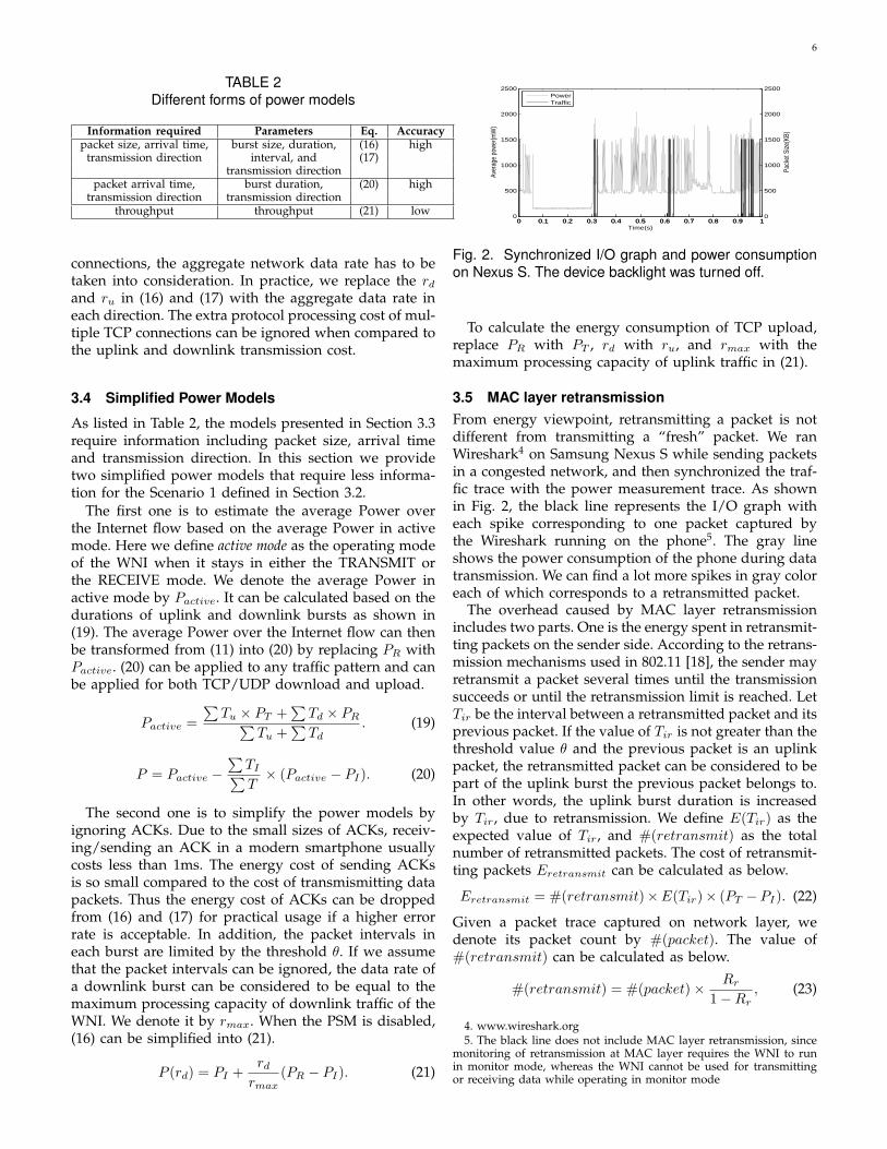
Fig. 2. Synchronized I/O graph and power consumptionon Nexus S. The device backlight was turned off.

To calculate the energy consumption of TCP upload,replace PR with PT , rd with ru, and rmax with themaximum processing capacity of uplink traffic in (21).

3.5 MAC layer retransmissionFrom energy viewpoint, retransmitting a packet is notdifferent from transmitting a “fresh” packet. We ranWireshark4 on Samsung Nexus S while sending packetsin a congested network, and then synchronized the traf-fic trace with the power measurement trace. As shownin Fig. 2, the black line represents the I/O graph witheach spike corresponding to one packet captured bythe Wireshark running on the phone5. The gray lineshows the power consumption of the phone during datatransmission. We can find a lot more spikes in gray coloreach of which corresponds to a retransmitted packet.

The overhead caused by MAC layer retransmissionincludes two parts. One is the energy spent in retransmit-ting packets on the sender side. According to the retrans-mission mechanisms used in 802.11 [18], the sender mayretransmit a packet several times until the transmissionsucceeds or until the retransmission limit is reached. LetTir be the interval between a retransmitted packet and itsprevious packet. If the value of Tir is not greater than thethreshold value θ and the previous packet is an uplinkpacket, the retransmitted packet can be considered to bepart of the uplink burst the previous packet belongs to.In other words, the uplink burst duration is increasedby Tir, due to retransmission. We define E(Tir) as theexpected value of Tir, and #(retransmit) as the totalnumber of retransmitted packets. The cost of retransmit-ting packets Eretransmit can be calculated as below.

Eretransmit = #(retransmit)×E(Tir)× (PT −PI). (22)

Given a packet trace captured on network layer, wedenote its packet count by #(packet). The value of#(retransmit) can be calculated as below.

#(retransmit) = #(packet)× Rr

1−Rr, (23)

4. www.wireshark.org5. The black line does not include MAC layer retransmission, since

monitoring of retransmission at MAC layer requires the WNI to runin monitor mode, whereas the WNI cannot be used for transmittingor receiving data while operating in monitor mode

7

where Rr is the retransmission ratio calculated fromMAC layer traffic information. For example, if we cap-ture N packets on MAC layer including M retransmis-sion attempts, the value of Rr is equal to M

N .The other part of the retransmission overhead is

caused by the increase in the baseline cost, due to theDynamic Voltage Frequency Scaling (DVFS) mechanismof CPUs. The basic idea of DVFS is to adapt the CPUfrequency to the processing workload. The extra work-load caused by retransmission may lead to an increase inthe CPU frequency, with the result that the baseline costrepresented by the values PT , PR, PI and PS increasesaccordingly. For example, in Fig. 2, the Power in theIDLE mode during 0.1s and 0.3s is only 0.177W, whereasit gets close to 0.5W during the interval between 0.8s and0.85s. Meanwhile, the Power while sending packets in-creases by around 0.3W when the retransmission starts.This change in Power is consistent with the change inthe CPU frequency from 100MHz to 200MHz. Hence,to estimate the transmission cost in congested networks,fine-grained CPU frequency measurement is necessaryfor providing the right inputs for the power models.

4 PRACTICAL ISSUES

The power models presented in Section 3 require twodifferent kinds of inputs. The first type are the hardwareparameters such as PT and PR, while the other type rep-resent the burst information derived from traffic traces.In this section we describe the methods of obtainingthe values of these inputs, and analzye the impact ofthese values on the resulting estimation accuracy ofour power models. We will leave the errors of powermeter calibration out of the scope of this work, and willfocus on the errors that come from the processing of thereadings obtained from power meters.

4.1 Measurement of Hardware ParametersWe measured the values of PT and PR and the maximumthroughput of the WNI while sending/receiving back-to-back packets. First, we sent fixed-size packets as fast aspossible from the phone at a given CPU frequency, andused the average power over a period (e.g. 60 seconds)as the corresponding value of PT . Second, we calculatedthe maximum uplink throughput as the packet sizedivided by the mean of the measured packet intervals.Similarly, we measured PR and the maximum downlinkthroughput while receiving packets to the phone.

We measured the power in the IDLE mode of theWNI, PI , by first transmitting packets from the device,and then measuring the power after stopping the trans-mission. On devices with the 802.11 PSM feature, theWNI went to the SLEEP mode after the PSM timeouthad passed from the stopping of the transmission, andwe could then measure the value of PS . On the deviceswith the DVFS feature, such as Samsung Nexus S, thehardware parameter values needed to be measured forall the possible CPU frequencies.

The way we measure PT and PR is based on theassumption that the WNI always stays in either theTRANSMIT or the RECEIVE mode during back-to-backpacket delivery. However, due to the delays causedby the data transmission over the air and the packetprocessing, true back-to-back packet delivery of packetsis not possible. This means that there always will besmall intervals between the packets, and it is possiblethat the WNI may switch into the IDLE mode duringthese small intervals. Because the power consumptionin the IDLE mode is lower than that in the TRANSMITor the RECEIVE modes, the measured power may belower than the correct value would be.

In order to analyze this measurement error in theTRANSMIT case, we denote the measured value of PT

with P′

T , the duration of the measurement with Tm, andthe actual duration spent in the IDLE mode during Tm

with Te. Now, the proportion d = Te

Tmgives an estimate of

the measurement error. Further, the relationship betweenthe correct PT and the measured P

′

T can be expressed as

P′

T =PT (1− d)Tm + PIdTm

Tm= PT − d(PT − PI). (24)

Similiar analysis can also be applied in the RECEIVEcase, but the equations are omitted due to space restric-tions.

4.2 Error in Power Estimation of Bursts

When using our power models for runtime power esti-mation, we make the assumption that the WNI alwaysstays in the TRANSMIT mode during uplink bursts, andin the RECEIVE mode during downlink bursts. Thisassumption is similar to the assumption that the WNIalways stays in either the TRANSMIT or the RECEIVEmode during back-to-back packet delivery, which wemade when measuring the hardware parameters. Thesimilarity of the assumptions implies that they mightalso carry a similar error source, and this is indeed thecase. Even within a burst, there are intervals between thepackets, and during these intervals the WNI may enterthe IDLE mode.

We now analyse this error in the case of uplink bursts,but the analysis can be trivially applied to downlinkbursts as well. The actual energy consumption of WNIduring the total duration of uplink bursts Tu consists oftwo parts, the energy spent in the TRANSMIT mode andthe energy spent in the IDLE mode during the packetintervals. We denote the proportion of the time spent inthe IDLE mode to Tu with d

′. The actual Power during

uplink bursts can be calculated following (25).

P =PT (Tu − d

′Tu) + d

′TuPI

Tu= PT − d

′(PT − PI). (25)

Because we use P′

T as the value of PT in our model-based power estimation, by comparing the values of P

′

T

and P we can get an estimate of the error in power

8

estimation of uplink bursts. We denote this error witheu, and it can be calculated following (26).

eu = P − P′

T = (d− d′)(PT − PI). (26)

Similar analysis can also be applied in analyzing ed,the error in power estimation of downlink bursts, byreplacing PT with PR and d

′with the proportion of the

time spent in the IDLE mode to Td in (26).

4.3 Impact of the Threshold ValueA packet trace can be divided into different numberof bursts with different packets included in each burst,depending on the value of the threshold θ that is usedfor burst detection. The distribution of packet intervalswithin bursts and further the value of d

′vary with the

value of θ. In an extreme case where the value of θ is0, each burst only includes one packet and the value ofd

′is 0. The probability of getting a higher value of d

′

increases with the value of θ. According to (26), if weincrease the value of θ starting from 0, the values of euand ed will first decrease until the value of d

′becomes

equal to that of d. After that, the values increase with θ.We define the MAPE of the power estimation of a flow

as below.

MAPE =|Pm − Pe|

Pm=

|euTu + edTd|PmTflow

(27)

where Pm is the measured power, Pe is the estimatedpower, and Tflow is the flow duration. The burst du-rations, Tu and Td, do not decrease with the value of θ.However, the values of eu and ed may decrease with θ, ifθ is small enough. In that case, the value of MAPE wouldincrease or not, depending on whether the increase in Tu

and Td can overtake the decrease in eu and ed. When θis big enough, the value of MAPE will always increasewith θ.

To evaluate these features, we take TCP down-load/upload on Samsung Nexus S as an example. Giventhe same set of packet traces and power measurementresults, we tune the value of θ and compare the resultingestimation accuracy. As shown in Fig. 3, the value ofMAPE first decreases together with the value of θ, andthen increases. The threshold value of 5ms providesgenerally the best accuracy for all the three cases. Ac-cording to our experience6, given the same values ofthe hardware parameters, a threshold value chosen tobe optimal for one of the test cases (e.g. concurrent TCPflows) usually also provides reasonable good accuracyin the other test cases as well.

5 EVALUATION

We chose TCP transmission as an example and evaluatedthe power models presented in Section 3 with physicalpower measurement on four smartphones, Nokia N810,

6. When evaluating the power models for Samsung Nexus S, we setthe value of θ to be 5ms for all the test cases.

1 2 3 4 5 6 7 8 9

10

3 4 5 6 8

MA

PE

(%)

Packet Interval Threshold(ms)

2 TCP download flows2 TCP upload flows1 TCP upload flow and 1 TCP download flow

Fig. 3. Comparison of MAPE with different thresholdvalues in the test case 4) defined in Table 3.

Fig. 4. Experimental setup.

Nokia N95, HTC G1 and Samsung Nexus S. As listedin Table 3, we evaluated our models in TCP transmis-sion scenarios at various data rates with various trafficpatterns and in different network environments. Morespecifically, we first conducted the experiments in anideal network environment where the processing latencyand packet loss can be ignored. We measured the powerconsumption of TCP download/upload with the datarate ranging from 16KBps to over 2MBps, and repeatedthe measurement with the data transmission using anumber of separate TCP flows. After that, we conductedTCP download/upload experiments in a congested net-work environment, with the retransmission ratio varyingbetween 10% and 30%. We also compared our estimationwith the physical measurement of four real Androidapplications. The traffic generated by these Androidapplications had different characteristics, in terms ofboth traffic size and pattern. The experimental setup andthe results of each test case are explained in this section.

5.1 Experimental SetupOur experimental setup is illustrated in Fig. 4, includingTCP download/upload setup, and power measurementand traffic capturing tools.

5.1.1 TCP download/upload setupWe used an open source TCP utility, netcat7, as theTCP server running on a Linux server, and our owncustom netcat-based mobile applications as the TCPclients. To avoid the energy cost of data copy operations,the downloaded files were written to /dev/null insteadof phone memories, and to the same end, the TCP clients

7. http://netcat.sourceforge.net/

9

TABLE 3List of test cases

No. Description No.flows Data rate limit TCP window scaling Phone models Equations1) TCP download/upload with PSM enabled 1 Enabled Disabled N810, N95 (17)2) TCP download/upload 1 Enabled Disabled N810,N95 (16)

HTC G13) TCP download/upload 1 Enabled/Disabled Enabled Nexus S (20)4) Concurrent TCP download/upload 2/4/8 Enabled/Disabled Enabled Nexus S (20)5) TCP download/upload in congested network 1 Enabled/Disabled Enabled Nexus S (22)6) Web browser, Fengxing(video streaming), 1 Disabled Enabled Nexus S (16),(17),

Dropbox(file upload), QQ(instant messenger) (21)

TABLE 4Experimental setup

Phone model OS Power meter Samplingfrequency

Nokia N810 Maemo 4.1 Fluke 189 logging 20Hz?multimeter

Nokia N95 Symbian S60 Nokia Energy Profiler 4HzHTC G1 Android 1.6 Fluke 189 logging 20Hz?

multimeterSamsung Android 2.3 Monsoon Power 5000HzNexus S Monitor9

? The logging interval in FlukeView is 1 second. The system logs theaverage of the 20 samples taken during each second.

on the phones generated all the data they uploaded on-the-fly instead of reading it from mass memory.

The TCP clients always try to send/receive data asfast as possible if no data rate limit is applied. In thatcase, the actual throughput is limited by the availablenetwork bandwidth and the processing capacity of thesmartphones. To conduct data transmission at a fixedrate, we ran Trickle [24], an utility for bandwidth throt-tling, on the same Linux server with the TCP server. Inaddition, apart from Nexus S, the TCP window scalingoption was disabled and the MTU was set to 1500 Bytes,so that the protocol processing cost for each packet couldbe considered to be fixed [25]. Moreover, disabling theTCP window scaling can increase the probability thatthe transmission rate would be limited by the receiverwindow, and hence, maximum window size would beused and that would generate bursts of equivalent size.

5.1.2 Power measurement

As described in Table 4, apart from Nokia N95, for whichwe used the power measurement software, Nokia En-ergy Profiler8, we connected all the other tested phonesto an external DC power supply and used physicalpower meters to measure the instant power consump-tion. The readings of the physical meters were loggedfrom the PC software provided by the manufacturers.

We measured the power consumption with the WNIoperating in different states, as described in Section 4.1.The results are listed in Tables 5 and 6. During themeasurements, only the basic components of the devices

8. http://www.developer.nokia.com/Resources/Tools anddownloads/Other/Nokia Energy Profiler/

TABLE 5Parameter values for N810, N95 and G1

Phone model Display PT (W) PR(W) PI (W) PS (W)Nokia N810 off 1.258 1.181 0.884 0.042Nokia N95 off 1.687 1.585 1.038 0.088

HTC G1 off 1.097 0.900 0.650 -

TABLE 6Parameter values for Nexus S

CPU Display PT (W) PR(W) PI (W) Data ratefrequency (KBps)100MHz off 1.094 0.867 0.177 ≤ 128100MHz off 1.130 0.903 0.213 160 - 256200MHz off 1.245 1.021 0.435 ≥ 512100MHz on 1.217 0.887 0.742 512200MHz on 1.376 1.050 0.800 1024400MHz on 1.549 1.208 0.890 ≥ 1536

were in use. We also note that the measured values of PT

and PR include the cost of network protocol processing.Because the Android phones we used did not provide

any interface for adjusting PSM parameters, we mea-sured them using the default settings. The measurementresults seem to fit the “PSM disabled” version of ourpower models. Therefore, we did not provide the valueof PS for these Android phones. In addition, we ob-served from Nexus S that its CPU frequency varied withthe transmission rate. For instance, when the display wasturned off, the CPU frequency increased from 100MHzto 200MHz whenever the data sending rate of the phoneincreased from 256KBps to 512KBps10. Therefore, we listin Table 6 the parameter values separately for each CPUfrequency. The listed data rate information is to showwhich values were used in our calculations. They arenot necessarily the exact thresholds used in DVFS.

5.1.3 Traffic capturingThe smartphones were connected to 802.11g accesspoints (APs) with beacon intervals set to 100ms. On thephones that support fine-tuning the PSM settings, NokiaN810 and N95, the PSM timeout was set to be 100ms.

During the experiments of TCP download/upload, thenetwork traffic was monitored by running Wiresharkon the Linux server that the smartphones connected to.

10. Due to the partial wake up mechanism in Android, the CPUworked at a reduced frequency when the display was turned off.

10

Except in the test case 5), the cross traffic in our APswas assumed to be insignificant. In the test case 5),we ran Kismet11 on a separate laptop to capture MAClayer traffic information from the WNI operating in themonitor mode. The captured information was later usedfor calculating MAC layer retransmission rate and theexpected value of the packet retransmission interval.

5.2 TCP download/upload with a Single FlowWe first evaluated our models with regularly repeatedbursty traffic. On N810, N95 and G1, we repeated TCPdownload/upload with data rate ranging from 16KBpsto 256KBps. The traffic was shaped by Trickle into regu-lar bursts with size of 4KB. As N810 and N95 supportsPSM, we measured their power consumption with PSMenabled and disabled, respectively. The measured valueswere compared with the model-based estimation fromthe traffic captured from the Linux server.

We empirically set the threshold value for burst de-tection in our models to be between 6 and 10ms, inorder to minimize the standard deviation of the detectedburst sizes. This allowed us to use 4KB as the data burstsize estimate for both TCP download and TCP upload.We calculated the average downlink and uplink burstdurations over the detected bursts. The burst durationsare listed in Table 7. For N810 and N95 that supportPSM, the burst size and duration information was usedfor calculating the threshold value of the network datarate rc, as described in (15). The value of rc was 37KBpsfor N810 and 36KBps for N95 in both TCP downloadand upload cases.

We estimated the transmission cost from the burstinformation and the parameter values listed in Table 5.The estimated values were calculated following (16) or(17), depending on which conditions of the two scenariosdefined in Section 3.2 were satisfied. The value of α in(17) was set to 2 when estimating the power consump-tion of N95 at the data rate of 16KBps12. In all othercases, it was set to 1.

On Nexus S we enabled the TCP window scaling toallow the burst sizes and burst intervals to vary. Weused the traffic traces collected from our Linux serveras input and calculated the aggregated energy cost withthe threshold value of burst definition set to 5 ms. Thisthreshold value was chosen as described in Section 4.3.We applied the model presented in (20) to estimate thepower consumption from the burst information and thehardware parameter values listed in Table 6.

11. http://www.kismetwireless.net/12. In the case of TCP download at 16KBps we observed from the

traffic trace of N95 that there were two uplink bursts in a bin withthe interval bigger than one PSM timeout. In the case of TCP uploadat 16KBps on N95, the intervals between ACK and the followingdata packet was longer than the ACK timeout, which caused theretransmission of ACK. The retransmission wakes up the WNI andincreases the duration spent in the IDLE mode. In both cases, theduration spent in the IDLE mode is longer than the PSM timeout, butno bigger than twice of the PSM timeout. For the sake of simplicity,we set the value of α to 2.

TABLE 7Burst durations observed on N810, N95 and G1

Test case Link N810(ms) N95(ms) G1(ms)TCP download downlink 8 10 10

uplink 0.5 0.35 0.5TCP upload uplink 6 12 8

downlink 0.1 0.2 0.1

TABLE 8MAPE of power models for N810, N95 and G1

Test case PSM N810 N95 G1TCP download On 4.3%±5.9% 4.9%±7.3% -

(single flow) Off 1.1%±0.7% 1.8%±2.9% 4.8%±2.7%TCP upload On 5.7%±4.9% 3.9%±5.5% -(single flow) Off 2.2%±1.7% 2.3%±2.3% 1.3%±1.4%

We compared the estimated Power with the physicalpower measurement, and measured the estimation accu-racy using MAPE as a metric. As listed in Table 8 and9, the average MAPE of TCP download/upload with asingle flow was at most 5.7%. We note that the results ofNexus S include the measurements in scenarios wherethe data is delivered with/without data rate limit.

We also calculated the energy utility for each test casefollowing (9). As shown in Fig. 5 and 6, the energy utilityof TCP download/upload is nearly proportional to thenetwork data rate. Thus it is more energy-efficient totransmit/receive data at a higher rate. In addition, whensending data at a rate lower than rc, it is more energy-efficient if the PSM is enabled.

5.3 TCP Download/Upload with Multiple Flows

Since there can be one or multiple TCP flows transferringdata from/to a mobile device, we extended our experi-ment from single TCP flow to multiple flows. Accordingto the burst definitions in Section 3, packets belongingto different TCP flows are included in the same burstif they satisfy the two conditions of packet interval andtransmission direction.

Assuming that there are N TCP flows running on onephone, we measured the power consumption of NexusS in the following three scenarios: 1. All N flows down-loading, 2. all N flows uploading, and 3. half of the flowsdownloading, other half uploading. For each scenario,we first ran the experiments without any data rate limit.After that, we used Trickle to set the limit of aggregatedata rate to various values ranging from 512KBps to2048KBps. The display was turned on with brightness setto 30% during the experiments. The experiments wererepeated with N set to 2, 4 and 8, respectively.

We estimated the Power following (20), using theaggregated traffic information as input. The MAPE ofour estimation was at most 9.1%, as shown in Table 9.We also calculated the mean and standard deviationof the energy utility at each data rate. Each data setcorresponding to a data rate included all the results fromthe experiments using 2, 4 and 8 TCP flows respectively.

11

10

15

20

25

30

35

40

45

50

16 16(PSM) 32 32(PSM) 16 16(PSM) 32 32(PSM)

Ene

rgy

Util

ity(K

B/J

)

Data rate(KB/s)

Measured(N810)Estimated(N810)

Measured(N95)Estimated(N95)

(a) On N810 and N95(16-32KBps).

40

60

80

100

120

140

160

180

200

220

240

64 96 128 160 192 224 256

Ene

rgy

Util

ity(K

B/J

)

Data rate(KB/s)

Measured(N810)Estimated(N810)Measured(N95)Estimated(N95)

(b) On N810 and N95(64-256KBps).

0

100

200

300

400

500

600

700

16 32 64 96 128 160 192 224 256

Ene

rgy

Util

ity(K

B/J

)

Data rate(KB/s)

Measured(G1)Estimated(G1)Measured(Nexus S)Estimated(Nexus S)

(c) On HTC G1 and Nexus S

Fig. 5. Energy utility of TCP download with single flow at rate between 16KBps and 256KBps.

10

15

20

25

30

35

40

45

50

16 16(PSM) 32 32(PSM) 16 16(PSM) 32 32(PSM)

Ene

rgy

Util

ity(K

B/J

)

Data rate(KB/s)

Measured(N810)Estimated(N810)

Measured(N95)Estimated(N95)

(a) On N95 and N810(16-32KBps).

40

60

80

100

120

140

160

180

200

220

240

260

64 96 128 160 192 224 256

Ene

rgy

Util

ity(K

B/J

)

Data rate(KB/s)

Measured(N810)Estimated(N810)Measured(N95)Estimated(N95)

(b) On N95 and N810(64-256KBps).

0

100

200

300

400

500

600

700

16 32 64 96 128 160 192 224 256

Ene

rgy

Util

ity(K

B/J

)

Data rate(KB/s)

Measured(G1)Estimated(G1)Measured(Nexus S)Estimated(Nexus S)

(c) On HTC G1 and Nexus S.

Fig. 6. Energy utility of TCP upload with single flow at data rate from 16KBps to 256KBps.

500

1000

1500

2000

2500

512 1024 1536 2048 2854(no-trickle)

Ene

rgy

Util

ity(K

B/J

)

Data rate(KBps)

MeasuredEstimated

(a) TCP download.

500

1000

1500

2000

2500

512 1024 1536 2048 2854(no-trickle)

Ene

rgy

Util

ity(K

B/J

)

Data rate(KBps)

MeasuredEstimated

(b) TCP upload.

500

1000

1500

2000

2500

512 1024 1536 2048 2854(no-trickle)E

nerg

y U

tility

(KB

/J)

Data rate(KBps)

MeasuredEstimated

(c) TCP download and upload.

Fig. 7. Energy utility of TCP download/upload on Nexus S. The X-axis represents the aggregated data rate of all theTCP flows. The biggest value on the X-axis is the maximum throughput achieved without any rate limit. Each datapoint shows the mean and the standard deviation of the measured or the estimated Power.

TABLE 9MAPE of power models for Nexus S

No. No. MAPE No. No. MAPEdownlink uplink (%) downlink uplink (%)

1 0 3.4±2.0? 0 1 2.6±1.5?4.2±1.7 4.1±4.4

2 0 3.3±1.7? 0 2 2.9±2.0?2.4±1.1 0 2 5.1±4.0

4 0 2.9±2.0 0 4 5.1±1.58 0 2.2±1.4 0 8 5.9±1.81 1 2.1±1.8? 1 1 2.7±1.92 2 5.0±2.8 4 4 4.8±2.1

? The display was turned off. The data rate was between 16 and256KBps.

As shown in Fig. 7, the standard deviation is very smallcompared to the value of the mean. As the processingoverhead for maintaining more TCP flows is includedin the measured Power, the small standard deviation ofthe measured Power shows that the processing overheadcan be safely ignored. Fig. 7 also shows that the powermodels presented in Section 3 can provide generally ac-curate energy estimation of TCP transmission, regardless

of the number of TCP flows.

5.4 TCP Download/Upload in Congested Network

We connected the Nexus S to a public AP in our cam-pus and measured the power consumption during TCPdownload and upload. The phone tried to send/receivedata as fast as possible without any data rate limit ortraffic shaping. Due to the interference caused by theneighbouring APs, MAC layer retransmissions couldnot be left ignored. Based on the collected MAC layertraffic traces, we calculated the retransmission ratio Rr

and the expected value of retransmitted packet intervalE(Tir). The samples of retransmitted packet intervalsused for calculating E(Tir) seem to follow the InverseGaussian distribution. The overhead of retransmittingpackets was computed following (22). Because the CPUfrequency was always 400MHz during the measurement,no extra cost was caused by DVFS. The final resultsare shown in Table 10. In upload cases, taking intoaccount the retransmission overhead can improve thepower estimation accuracy by almost 50%.

12

TABLE 11Description of the experiments with Android apps

App Description Display Throughput(KBps) Duration(s) App overhead(mW)? MAPEFengxing video player Stream videos from youku.com on 7.9 3054 103 5.4%Dropbox android app Upload files to dropbox.com on 18.9 1578 112 5.3%

Web browser Open web pages on dalong.net off 13.8 509 41 4.3%QQ instant messenger Receive random text messages off 0.04 1068 127 8.6%

? when the CPU is active

TABLE 10MAPE of power estimation in congested networks

Test case Rr(%) E(Tir)(ms) MAPE(%)Download 11.2±1.5 - 2.4±1.2

Upload 20.6±2.3 0.8±0.2 5.2±4.1 (11.0±1.4?)? The retransmission overhead is not counted.

5.5 Real life applicationsWe evaluated the accuracy of the complete power mod-els (Eq.(16), (17)), and the simplified one (Eq.(21)) withfour real-life applications running on Nexus S. Accord-ing to our measurements, the phone does not seem toimplement the traditional 802.11 PSM/PSM adaptivewith the WNI SLEEP mode, but does instead have aDVFS-induced low-power state that is entered uponexpiration of an inactivity timer. This mechanism worksin a manner similar enough to the 802.11 PSM that Eq.(17) can be applied with good results by replacing PS

with the measured power of the DVFS-induced low-power state, and the value of PSM timeout with thelength of the inactivity timer.

The descriptions of the tested applications are listed inTable 11 along with experiment parameters and results.During the experiments, we ran Wireshark directly onthe phone to capture the network layer traffic traces. Thepacket interval threshold used for burst detection wasset to 5ms, and the overhead caused by the applicationsthemselves13 was included in the estimated values. Wedetermined empirically the length of the inactivity timerto be about 1.35s when the display was off, and to be400ms when the display was on. As shown in Fig. 8, allthe models gave reasonable results, except in the caseof the QQ messenger where only model (17) was able toestimate the power with good accuracy. This was causedby the exceptionally long burst intervals in the QQmessenger traffic, during which the DVFS put the phoneinto the low-power-state, which was only accounted forin model (17). Indeed, the traffic generated by the other3 applications had at least 87% of the burst intervalsshorter than 400ms. In the case of QQ messenger, only21% of burst intervals were shorter than 400ms, whilethe WNI was estimated to stay in the SLEEP mode formore than 22% of the burst intervals.

5.6 Comparsion with PowerTutorWe chose the test case 3) defined in Table 3 as exampleand compared the accuracy of our approach with that

13. Measured Power with the app running without any data transfer.

of the readings from the PowerTutor [11] Android ap-plication. From Fig. 9 and 10 we can see that whereasthe estimations of our model closely predict the mea-sured values, the original PowerTutor readings deviatefrom the absolute measured values, and fail to followthe trends seen in the physical measurement. The higherror rate can be explained by the fact the PowerTutormodels had not been trained for the device in question(Nexus S), with the result that the value of the hardware-specific parameter Pbaseline might have been incorrect.Additionally, PowerTutor did not take into account theimpact of CPU DVFS on the baseline power consump-tion. To reduce the bias caused by inaccurate Pbaseline,we calibrated PowerTutor by configuring the value ofPbaseline, which is hardcoded in the PowerTutor androidapplication, with the values of PI listed in Table 6. Whenthe display was turned on, the PowerTutor androidapplication estimated the power consumption of thedisplay to be 183.6mW in our test cases. Because thepower consumption of the display if available is alreadyincluded in the value of PI , we deducted 183.6mW fromthe calibrated results of PowerTutor in cases where thedisplay was turned on.

Although the calibrated results of PowerTutor pro-vided much better accuracy than the original ones, theystill under-estimated the proportional effect of data rateon the power consumption. The MAPE of the calibratedPowerTutor readings is 20.74±12.96% in download casesand 12.93±10.86% in upload cases, which is higher thanthe MAPE of our models as listed in Table 9. This mightindicate that the Wi-Fi power model of PowerTutor thataccording to [11] only takes into account the packetrate and the uplink channel rate as measured variablesis too minimalistic to accurately describe the powerconsumption behaviour of real-life data transfer, whereother variables such as traffic shape and CPU frequencyalso matter.

6 DISCUSSIONThe most recently commercialized standard 802.11nfeatures several new features and enhancements com-pared to 802.11g. These features include MIMO support,channel bonding, and two power-saving mechanisms,namely Spatial Multiplexing Power Save (SMPS) andPower Save Multi-Poll (PSMP).

MIMO can be used either for spatial diversity bysimultaneously transmitting redundant data streams en-coded in a special way in order to increase range and ro-bustness of data transmission or for spatial multiplexing

13

0

0.15

0.3

0.45

0.6

0.75

0.9

1.05

Fengxing Dropbox Web Browser QQ

Pow

er(W

)Measured

Estimated(Eq.(16))Estimated(Eq.(21))Estimated(Eq.(17))

Fig. 8. Power consumption of 4 An-droid applications on Nexus S.

0

0.2

0.4

0.6

0.8

1

1.2

1.4

1.6

16 32 64 96 128 224 256 512 1024 1536

Pow

er(W

)

Data rate(KB/s)

MonsoonPowerTutor(Original)PowerTutor(Calibrated)Our Approach

Fig. 9. Power consumption of TCPdownload with single flow on Nexus S.

0

0.2

0.4

0.6

0.8

1

1.2

1.4

1.6

16 32 64 96 128 224 256 512 1024 1536

Pow

er(W

)

Data rate(KB/s)

MonsoonPowerTutor(Original)PowerTutor(Calibrated)Our Approach

Fig. 10. Power consumption of TCPupload with single flow on Nexus S.

by transmitting multiple separate spatial data streamssimultaneously in order to increase the transmission rate.In [26], the authors measured the energy consumptionof 802.11n and discovered that only the number ofactive RF chains has a significant impact on the powerdraw and it does not matter much whether they areused for spatial diversity or multiplexing. Therefore, itis necessary to add the number of RF chains active ata given time instant as a parameter to capture MIMOcharacteristics in a power model.

Channel bonding allows to combine two adjacent 20MHz channels into a single 40 MHz channel therebydoubling the bandwidth and transmission rate. Usinga wider channel in this way has negligible impact onpower consumption according to [26], which means thatthis feature can be also neglected by power models.

SMPS and PSMP do not alter the basic behaviour ofthe power saving mechanism of 802.11. Both reduce theenergy consumed during idle periods. SMPS reduces thepower draw when client is not receiving by switching offall but one RF chain. PSMP effectively makes it possiblefor the client to sleep as much of the idle time as possible.Considering our models, the impact of both of thesemechanisms is reflected in the power levels measuredfor idle and sleep states and do not require specificmodifications to the models.

The upcoming 802.11ac standard promises data ratesbeyond a gigabit per second which are achieved bytaking advantage of more of the same above mentionedfeatures of 802.11n. Specifically, 802.11ac can use widerchannels (up to 160 MHz) and up to 8 spatial streams forMIMO operations. Thus, we have reason to expect thatthe same modelling approach will work for this familyof products as well.

Our power models would serve well also in networksimulators, such as NS-3. Integrating the models intosuch discrete event simulators is possible since the basicinput to the models, namely packet headers, are readilyavailable in such simulators. However, the support foraccurate node models is presently limited [27]. For thisreason, it is not possible to directly obtain DVFS relatedinformation of the simulated node. However, the differ-ent CPU frequency and voltage levels could be mappedto other measurable variables such as MAC level frametransmission/reception rate which the authors in [28]found to be highly accurate. Such mapping requires

specific calibration for each different node device.

7 CONCLUSION

In this paper we present accurate and practical powermodels of Wi-Fi data transmission in infrastructuremode. To the best of our knowledge, our work is the firstone that introduces traffic burstiness into power model-ing of Wi-Fi data transmission. Our models quantify theimpact from traffic patterns and network performance onthe transmission cost, mainly caused by the operationsof the WNI. These models can be used for estimating thepower consumption of various network applications thatare implemented with one to multiple TCP/UDP flowswhile being executed in varying network environments.We evaluate our models with physical power mea-surement of TCP-based data transmission on Maemo,Symbian and Android phones. The experimental re-sults show that the MAPE of our power models isat most 9.1%, which is high enough for practical use.Furthremore, the characteristics of the transmission costrevealed in our power models do provide necessarymotivation and insight into new solutions of energy-efficient Wi-Fi data transmission.

REFERENCES

[1] F. Qian, Z. Wang, A. Gerber, Z. Mao, S. Sen, and O. Spatscheck,“Profiling resource usage for mobile applications: A cross-layerapproach,” in Proc. of MobiSys ’11, June 2011, pp. 321–334.

[2] R. Friedman, A. Kogan, and K. Yevgeny, “On power and through-put tradeoffs of wifi and bluetooth in smartphones,” in Proc. ofINFOCOM’11, April 2011, 2011.

[3] M. Hoque, M. Siekkinen, and J. K. Nurminen, “On the energyefficiency of proxy-based traffic shaping for mobile audio stream-ing,” in Proc. of CCNC ’11, January 2011, pp. 891–895.

[4] A. Saarinen, M. Siekkinen, Y. Xiao, J. K. Nurminen, M. Kemp-painen and P. Hui, “Can offloading save energy for popularapps?,” in Proc. of MobiArch ’12, August 2012, pp. 3–10.

[5] E. Cuervo, A. Balasubramanian, D.-k. Cho, A. Wolman, S. Saroiu,R. Chandra, and P. Bahl, “Maui: Making smartphones last longerwith code offload,” in Proc. of MobiSys ’10, June 2010, pp. 49–62.

[6] E. Tan, L. Guo, S. Chen, and X. Zhang, “Psm-throttling: Minimiz-ing energy consumption for bulk data communications in wlans,”in Proc. of ICNP’07, October 2007, pp. 123–132.

[7] S. Mohapatra, N. Dutt, A. Nicolau, and N. Venkatasubramanian,“Dynamo: A cross-layer framework for end-to-end qos and en-ergy optimization in mobile handheld devices,” IEEE J. Select.Areas Commun, vol. 25, no. 4, pp. 722–737, May 2007.

[8] J. Garcia-Dorado, A. Finamore, M. Mellia, M. Meo, and M. Mu-nafo, “Characterization of isp traffic: Trends, user habits, andaccess technology impact,” Network and Service Management, IEEETransactions on, vol. 9, no. 2, pp. 142 –155, June 2012.

14

[9] Y. Xiao, P. Savolainen, A. Karppanen, M. Siekkinen, and A. Yla-Jaaski, “Practical power modeling of data transmission over802.11g for wireless applications,” in Proc. of e-Energy ’10, April2010, pp. 75–84.

[10] J. Flinn and M. Satyanarayanan, “Managing battery lifetime withenergy-aware adaptation,” ACM Trans. Comput. Syst., vol. 22, pp.137–179, May 2004.

[11] L. Zhang, B. Tiwana, Z. Qian, Z. Wang, R. P. Dick, Z. M. Mao, andL. Yang, “Accurate online power estimation and automatic batterybehavior based power model generation for smartphones,” inProc. of CODES/ISSS ’10, October 2010, pp. 105–114.

[12] M. Dong and L. Zhong, “Self-constructive high-rate system en-ergy modeling for battery-powered mobile systems,” in Proc. ofMobiSys ’11, June 2011, pp. 335–348.

[13] Y. Xiao, R. Bhaumik, Z. Yang, M. Siekkinen, P. Savolainen, andA. Yla-Jaaski, “A system-level model for runtime power estima-tion on mobile devices,” in Proc. of GreenCom ’10, Dec. 2010, pp.27–34.

[14] A. Pathak, Y. C. Hu, M. Zhang, P. Bahl, and Y.-M. Wang, “Fine-grained power modeling for smartphones using system call trac-ing,” in Proc. of EuroSys ’11, April 2011, pp. 153–168.

[15] H. Singh, S. Saxena, and S. Singh, “Energy consumption of tcp inad hoc networks,” Wirel. Netw., vol. 10, pp. 531–542, Sep. 2004.

[16] F. Qian, Z. M. Mao, Z. Wang, S. Sen, A. Gerber, and O. Spatscheck,“Characterizing radio resource allocation for 3g networks,” inProc. of IMC ’10, Nov. 2010, pp. 137–150.

[17] J. Huang, F. Qian, A. Gerber, Z. M. Mao, S. Sen, and O. Spatscheck,“A close examination of performance and power characteristics of4g lte networks,” in Proc. of MobiSys ’12. June 2012, pp. 225–238.

[18] “IEEE Standard for Information Technology - Telecommunica-tions and Information Exchange Between Systems - Local andMetropolitan Area Networks - Specific Requirements - Part 11:Wireless LAN Medium Access Control (MAC) and Physical Layer(PHY) Specifications,” IEEE Std 802.11-2007 (Revision of IEEE Std802.11-1999), pp. C1 –1184, June 2007.

[19] R. Fonseca, P. Dutta, P. Levis, and I. Stoica, “Quanto: Trackingenergy in networked embedded systems,” in Proc. of OSDI’08,Dec. 2008, pp. 323–338.

[20] B. Wang and S. Singh, “Analysis of tcp’s computational energycost for mobile computing,” SIGMETRICS Perform. Eval. Rev.,vol. 31, pp. 296–297, June 2003.

[21] H. Jiang and C. Dovrolis, “Why is the internet traffic bursty inshort time scales?” in Proc. of SIGMETRICS ’05, June 2005, pp.241–252.

[22] L. Guo, X. Ding, H. Wang, Q. Li, S. Chen, and X. Zhang, “Ex-ploiting idle communication power to improve wireless networkperformance and energy efficiency,” in Proc. of INFOCOM’06,April 2006, pp. 1–12.

[23] K.-c. Lan and J. Heidemann, “A measurement study of correla-tions of internet flow characteristics,” Comput. Netw., vol. 50, no. 1,pp. 46–62, 2006.

[24] M. A. Eriksen, “Trickle: A userland bandwidth shaper for unix-like systems,” in Proc. of USENIX ATC’ 05, April 2005, pp. 61–70.

[25] S. Agrawal and S. Singh, “An experimental study of tcp’s energyconsumption over a wireless link,” in Proc.of EPMCC’01, 2001.

[26] D. Halperin, B. Greenstein, A. Sheth, and D. Wetherall, “Demys-tifying 802.11n power consumption,” in Proc. of HotPower’10, Oct.2010.

[27] S. Kristiansen, T. Plagemann, and V. Goebel, “Towards scalableand realistic node models for network simulators,” SIGCOMMComput. Commun. Rev., vol. 41, no. 4, pp. 418–419, Aug. 2011.

[28] A. Garcia-Saavedra, P. Serrano, A. Banchs, and G. Bianchi, “En-ergy consumption anatomy of 802.11 devices and its implicationon modeling and design,” in Proc. of CoNEXT ’12, Dec. 2012, pp.168–180.

Yu Xiao received the PhD degree in com-puter science from Aalto University in 2012.She is currently a postdoc researcher at thedepartment of computer science and engineer-ing, Aalto University. Her current research inter-ests include energy-efficient wireless network-ing, crowd-sensing and mobile cloud computing.

Yong Cui Ph.D., Professor in Tsinghua Univer-sity, Council Member in China CommunicationStandards Association, Co-Chair of IETF IPv6Transition WG Softwire. Having published morethan 100 papers in refereed journals and confer-ences, he is also the winner of Best Paper Awardof ACM ICUIMC 2011 and WASA 2010. Hismajor research interests include mobile wirelessInternet and computer network architecture.

Petri Savolainen received his M.Sc from Uni-versity of Helsinki in 2004. He is currently apost-graduate student at department of com-puter science, University of Helsinki and also aresearcher at Helsinki Institute for InformationTechnology. His current research interests in-clude peer-to-peer networking, energy-efficientcomputing, and mesh networking.

Matti Siekkinen obtained M.Sc. in computerscience from Helsinki University of Technologyand in Networks and Distributed Systems fromUniversity of Nice Sophia-Antipolis in 2003, andPh.D from Eurecom / University of Nice Sophia-Antipolis in 2006. He is currently a senior re-search scientist at the department of computerscience and engineering, Aalto University. Hisresearch interests include energy efficiency inICT, network measurements, and Internet pro-tocols.

An Wang received B.Sc in computer sciencefrom Beijing University of Posts and Telecommu-nications in 2010. He is currently pursing M.Sc.His research interests include energy-efficientwireless networking.

Liu Yang is an undergraduate student from Bei-jing JiaoTong University. Her research interestsinclude energy-efficient wireless networking.

Antti Yla-Jaaski received his PhD in ETHZuerich 1993. Antti has worked with Nokia 1994-2009 in several research and research man-agement positions with focus on future Inter-net, mobile networks, applications, services andservice architectures. He has been a professorfor Telecommunications Software, Departmentof Computer Science and Engineering, AaltoUniversity since 2004. His current research in-terests include green ICT, mobile computing,service and service architecture.

Sasu Tarkoma received his M.Sc. and Ph.D. de-grees in Computer Science from the Universityof Helsinki, Department of Computer Science.He is full professor at University of Helsinki,Department of Computer Science and Head ofthe networking and services specialization line.He has over 100 scientific publications, and hasauthored three books. His interests include mo-bile computing, Internet technologies, and mid-dleware.