Modeling Drilling & Fluidization

Processes with DEM

Alex Read, Dr Oleh Baran

DEM for modeling rock drilling

– Breaking rock challenges

– Relevant capabilities in STAR-CCM+®

– Example without coupling to fluid flow

– Using overset mesh to model drill-bit motion

DEM for modeling flow of solids in fluidized beds

– Coarse-grain model in STAR-CCM+

– Industrial scale fluidized bed example

• Simulation results for large particle size distribution

Summary

Outline

2

Rock Cutting Complexity

Rock cutting:

– Complex non-equilibrium and non-

steady-state processes

– Wide range of length-scales

• From grain scale

• To bore-hole / reservoir dimensions

– Wide range of time-scales

• From sound waves period in solids

• To hours of advancing drill-bit

through inhomogeneous rock

Can numerical modeling help?

– In improving drill-bit design

– In optimizing operation parameters

(rpm, ROP, WOB)

– Reduce bit balling

3

Modeling Rock using DEM

DEM models individuals grains in

rock

– Accurate grain scale physics

• Resolution of grains-cutter contacts

• Can reproduce removing cuttings

– Limited to smaller length scales

and timescales

Model inputs

– Bit Design

• Nozzle selection

• Teeth configuration, etc

– Operation parameters

• Weight on Bit (or ROP), RPM…

– Rock properties

Observables

– Rate of penetration (or WOB)

– Torque

– Cuttings attached to drill bit

– Stand pipe pressure

Model challenges

– Simulation time

– Far Boundaries

– Calibrating model of rock

– Simulating flow of drilling fluid in borehole

– Reproducing bit balling

– Reproducing realistic cutting flows

4

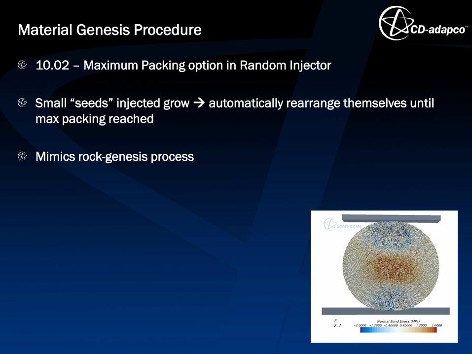
10.02 – Maximum Packing option in Random Injector

Small “seeds” injected grow automatically rearrange themselves until

max packing reached

Mimics rock-genesis process

Material Genesis Procedure

The Parallel Bonds model introduces attractive inter-particle forces to the particle system

Model uses the concept of a massless bar connecting a pair of bonded particles

The bar(bond) can transmit force and torque between particles and it is also subject to breaking under load

– The stress limit values are calculated based on beam theory

Reference: Potyondy, D.O, and Cundall, P.A. 2004. “A bonded-particle model for rock”, Int. J. Rock Mechanics & Mining Sciences 41 pp. 1329–1364.

DEM Parallel Bonds Model in STAR-CCM+

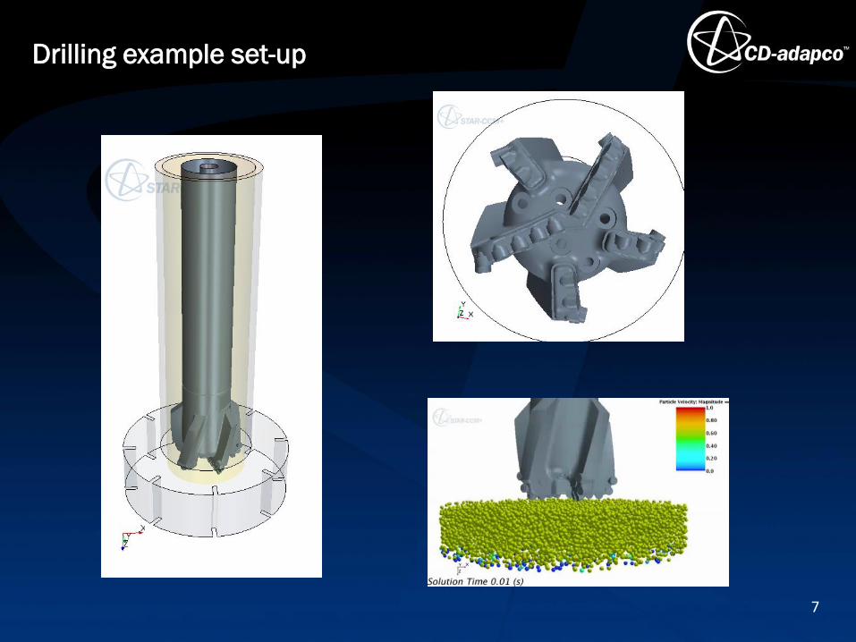
Drilling example set-up

7

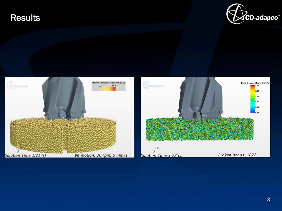
Results

8

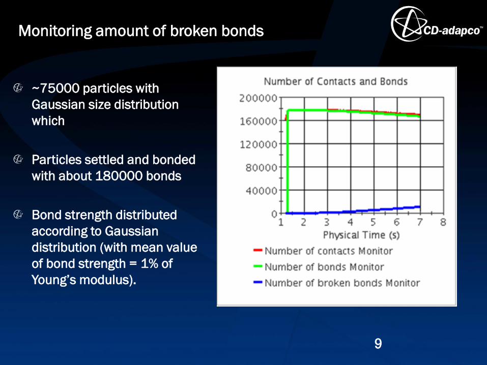
~75000 particles with

Gaussian size distribution

which

Particles settled and bonded

with about 180000 bonds

Bond strength distributed

according to Gaussian

distribution (with mean value

of bond strength = 1% of

Young’s modulus).

Monitoring amount of broken bonds

9

Contact network

10

Contact colored by ‘Bond State’

11

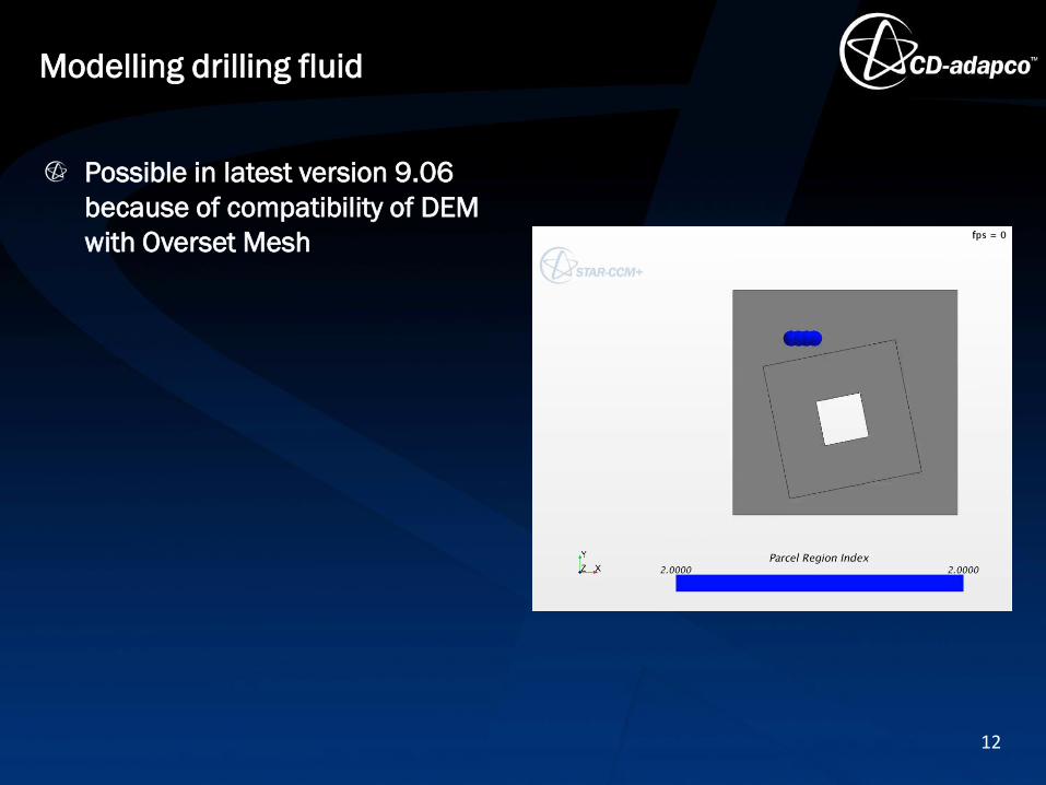
Modelling drilling fluid

Possible in latest version 9.06

because of compatibility of DEM

with Overset Mesh

12

Results with overset mesh

Rock is permeable with void

fraction =0.4

Solution for drilling fluid flow was

obtained using 2-way coupling

model

Jet flow form nozzles results in

large drag forces on bonded

grains

13

After drilling – before Chemical processing

14

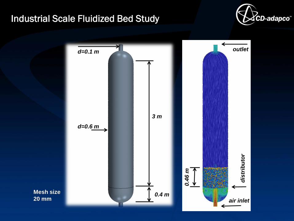
Industrial Scale Fluidized Bed Study

15

3 m

d=0.6 m

0.4 m

d=0.1 m

0.4

6 m

outlet

air inlet

dis

trib

uto

r

Mesh size

20 mm

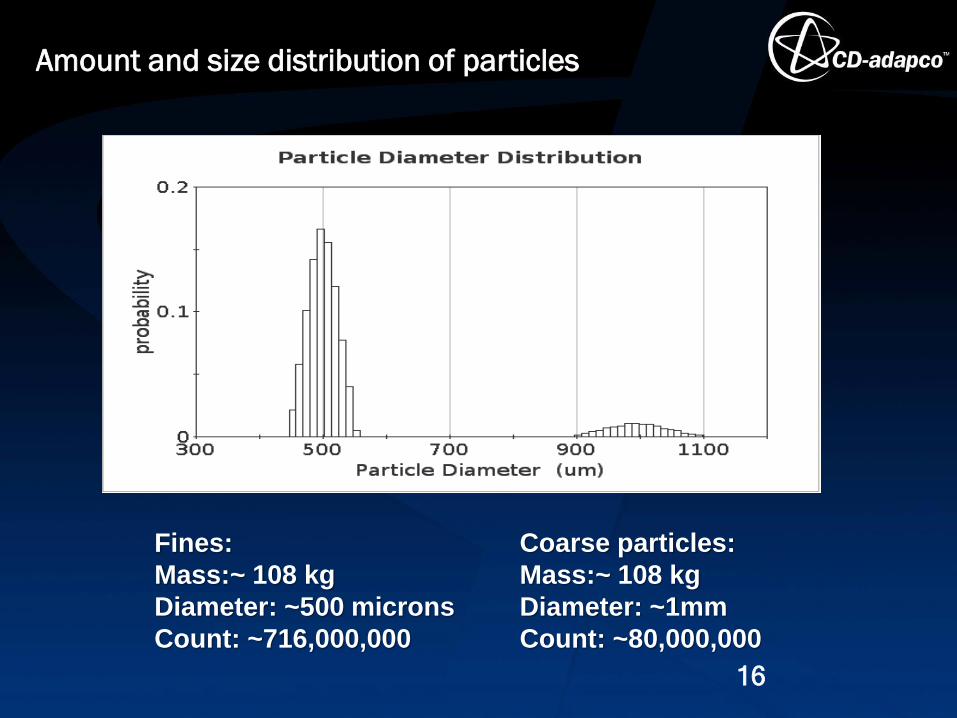
Amount and size distribution of particles

16

Fines:

Mass:~ 108 kg

Diameter: ~500 microns

Count: ~716,000,000

Coarse particles:

Mass:~ 108 kg

Diameter: ~1mm

Count: ~80,000,000

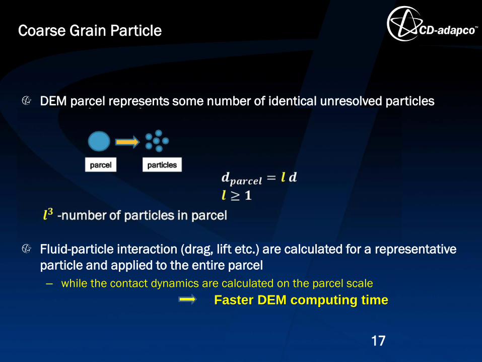
DEM parcel represents some number of identical unresolved particles

dparcel

l3 -number of particles in parcel

Fluid-particle interaction (drag, lift etc.) are calculated for a representative

particle and applied to the entire parcel

– while the contact dynamics are calculated on the parcel scale

Coarse Grain Particle

17

particlesparcel

Faster DEM computing time

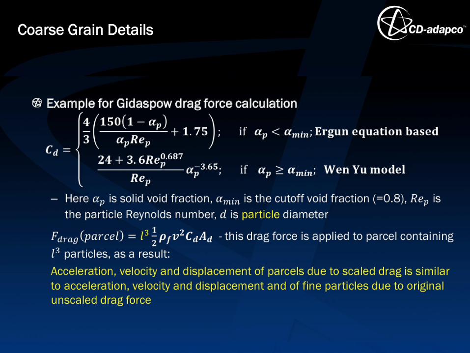
Example for Gidaspow drag force calculation

𝑪𝒅 =

𝟒

𝟑

𝟏𝟓𝟎 𝟏 − 𝜶𝒑

𝜶𝒑𝑹𝒆𝒑+ 𝟏. 𝟕𝟓 ; if 𝜶𝒑 < 𝜶𝒎𝒊𝒏; 𝐄𝐫𝐠𝐮𝐧 𝐞𝐪𝐮𝐚𝐭𝐢𝐨𝐧 𝐛𝐚𝐬𝐞𝐝

𝟐𝟒 + 𝟑. 𝟔𝑹𝒆𝒑𝟎.𝟔𝟖𝟕

𝑹𝒆𝒑𝜶𝒑

−𝟑.𝟔𝟓; if 𝜶𝒑 ≥ 𝜶𝒎𝒊𝒏; 𝐖𝐞𝐧 𝐘𝐮 𝐦𝐨𝐝𝐞𝐥

– Here 𝛼𝑝 is solid void fraction, 𝛼𝑚𝑖𝑛 is the cutoff void fraction (=0.8), 𝑅𝑒𝑝 is the

particle Reynolds number, 𝑑 is particle diameter

𝐹𝑑𝑟𝑎𝑔 𝑝𝑎𝑟𝑐𝑒𝑙 = 𝑙3𝟏

𝟐𝝆𝒇𝒗

𝟐𝑪𝒅𝑨𝒅 - this drag force is applied to parcel containing 𝑙3

particles, as a result:

Acceleration, velocity and displacement of parcels due to scaled drag is similar to

acceleration, velocity and displacement and of fine particles due to original

unscaled drag force

Coarse Grain Details

18

Parcel Size distribution

19

Fine:

9 mm; 109,000

Coarse:

18 mm; 14,000

Fine:

12 mm; 46,000

Coarse:

12 mm; 46,000

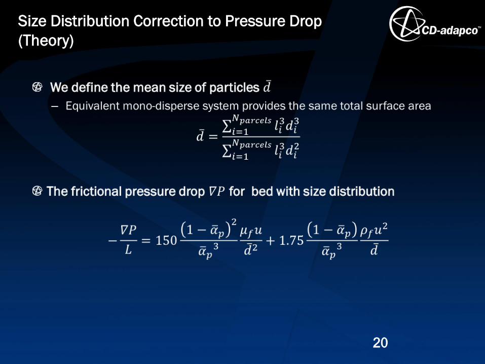
We define the mean size of particles 𝑑

– Equivalent mono-disperse system provides the same total surface area

𝑑 =

𝑖=1

𝑁𝑝𝑎𝑟𝑐𝑒𝑙𝑠 𝑙𝑖3𝑑𝑖

3

𝑖=1

𝑁𝑝𝑎𝑟𝑐𝑒𝑙𝑠 𝑙𝑖3𝑑𝑖

2

The frictional pressure drop 𝛻𝑃 for bed with size distribution

−𝛻𝑃

𝐿= 150

1 − 𝛼𝑝2

𝛼𝑝3

𝜇𝑓𝑢

𝑑2+ 1.75

1 − 𝛼𝑝

𝛼𝑝3

𝜌𝑓𝑢2

𝑑

Size Distribution Correction to Pressure Drop

(Theory)

20

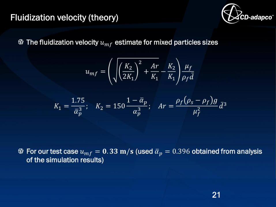
The fluidization velocity estimate for mixed particles sizes

For our test case (used obtained from analysis of the simulation results)

Fluidization velocity (theory)

21

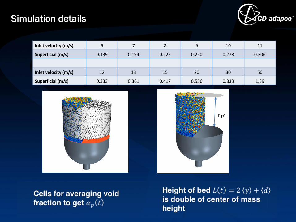
Inlet velocity (m/s) 5 7 8 9 10 11

Superficial (m/s) 0.139 0.194 0.222 0.250 0.278 0.306

Inlet velocity (m/s) 12 13 15 20 30 50

Superficial (m/s) 0.333 0.361 0.417 0.556 0.833 1.39

Simulation details

22

L(t)

Cells for averaging void

fraction to get

Height of bed 𝐿 𝑡 = 2 𝑦 + 𝑑is double of center of mass

height

Results for bed height and void fraction

23

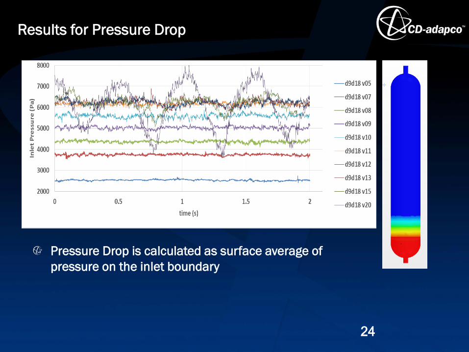
Pressure Drop is calculated as surface average of

pressure on the inlet boundary

Results for Pressure Drop

24

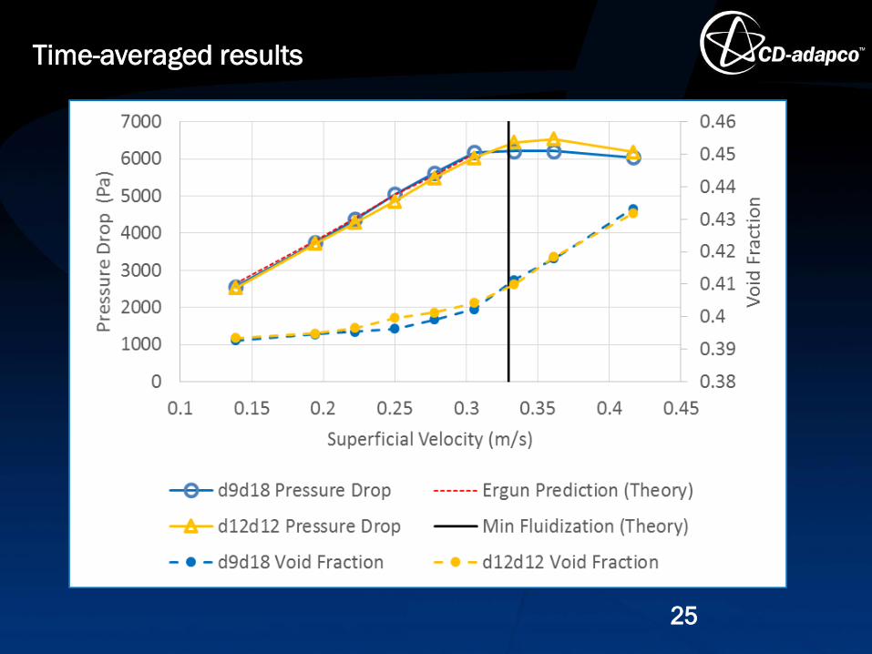
Time-averaged results

25

Fluidization Animations d9d18

26

0.25 m/s 0.31 m/s 0.33 m/s 0.36 m/s 0.56 m/s

Superficial = 1.39 m/s

Freeboard

27

d9d18 d12d12

Segregations

28

d9d18 d12d12

Summary

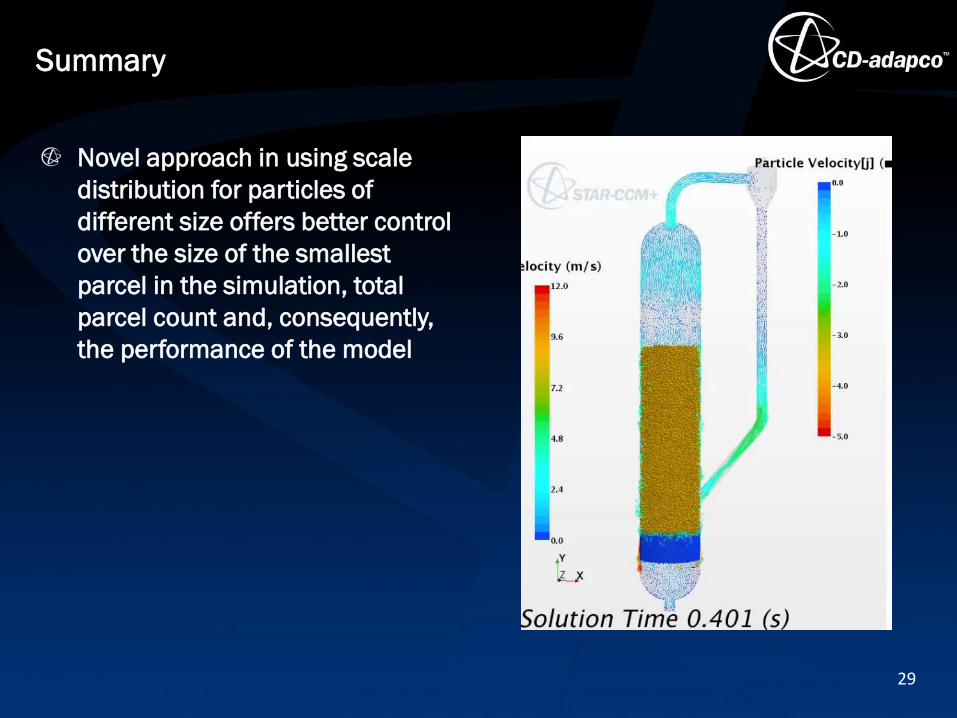
Novel approach in using scale

distribution for particles of

different size offers better control

over the size of the smallest

parcel in the simulation, total

parcel count and, consequently,

the performance of the model

29