modeling, development, and testing of an integral dose...
TRANSCRIPT

IIS Integrated Systems Laboratories & DEI Department of Information Engineering
Modeling, Development, and Testing of an Integral Dose
Calorimeter for the Characterization of Electron Beam
Crosslinking Processes in Industrial Environment
Supervisor UNIPD: Prof. Gaudenzio Meneghesso
Supervisor ETHZ: Dr. Mauro Ciappa, Dipl. Phys. Luigi Mangiacapra
Master Student: Alexandra Lupi
Matriculation Number: 601512 – IL
Master Degree in Electrical Engineering
Academic Year 2009-2010


1
Diplomarbeit im Studiengang Elektrotechnik und Informationstechnologie
Frühling 2010
für
Alexandra LUPI E ras m u s s tu d e n t (U n ive rs ity of Pad ova, Italy)
Modeling, Development, and Testing of an Integral Dose C alorimeter for the C haracterizationof Electron
Beam C rosslinking Processes in Industrial Environment Supervisor ETH Z: D r. M auro C iappa, D ipl. Phys. Luigi M angiacapra Supervisor U NIPD : Prof. Gaudenzio M eneghesso, U nivers ity of Padova Ausgabe: February 22, 2010 Abgabe: August 27, 2010
Institut für Integrierte Systeme Integrated Systems Laboratory

2
I . Introduction One among the main challenges in electron beam processing of polymers is the set up the ideal irradiation conditions to deliver a uniform dose in the isolation layer of cables and thus to obtain the best degree of polymer crosslinking, which satisfy the required specifications. At the IIS, this problem is solved by three-dimensional Monte Carlo simulation. Together with the accelerator geometry, electron beam energy is one of the main parameters that affect the final dose uniformity. During processing, cables are span through dedicated conveyors and pass several times across the irradiation field in different positions and fluence values. This involves several irradiations with different spatial dose distributions. For a fine dose calculation, the simulation has to be subdivided into multiple steps to reproduce the real geometry. Then, all contributions are added to obtain the spatial distribution of the cumulated dose. For this scope, a three-dimensional Monte Carlo simulation flow is used to calculate automatically the cumulated dose distribution for accelerator geometries of whatever complexity.
An iterative procedure have been already developed to calculate the beam energy for optimum dose uniformity. As usual in Monte Carlo simulations, the calculation time can become a relevant issue, unless proper parallelization schemes are used, which make possible to produce a solution within some few minutes.
In this framework, a major challenge is the calibration of Monte Carlo models by suitable experi-mental procedures.
II . Purpose The present master thesis work consists of a first part, where an integral dose calorimeter has to be designed and manufactured, and of a second part, where the calorimeter is used in an in-dustrial plant to measure the average energy of the electrons imping at the surface of the target.
In the first part, the material (e.g. C, Cu, Al H2O, Polyethylene), the size, and the time constant of the calorimeter has to be optimized on the base of transient thermal (Ansys Workbench 14.0) and dose deposition (EBXLINK 1D/3D) simulations. A design has to be chosen that minimizes the heat losses and the electron energy absorption through the barrier layers. The sources of systematic errors have to be identified and procedures to correct the measurement developed accordingly. The overall measurement error after correction of the systematic contribution has to be less than 1%. The temperature acquisition system (datalogger, acquisition software, temperature sensor) has to be configured to cope with these specifications. Drawings have to be available as in a suit-able form in order to be manufactured at the D-ITET workshop.
In the second part, measurements will be perfomed at an industrial plant, with the scope to assess the performance of the developed system. Cables and electronic systems have to be shielded properly in order to avoid degration through the ambient radiation (high energy electrons, X-rays). The obtained data have to processed and represented according to the standard protocols.

3
I I I . Tasks The task breakdown of present Thesis work is as follows:
1. Get acquainted with the thermal simulator Ansys Workbench 14.0 and with EBXLINX1D/3D. Calculate the time to the steady-state for different materials (eventually by using also compact thermal models), geometries based on realistic dose distributions in the absorber.
2. Optimize the system design, in particular taking into account
a. Package
b. Absorber (material, geometry)
c. Thermal isolation
d. Select datalogger and related control software
e. Select temperature sensor
f. Conceive a dedicated forced convection system in the case of the water calorimeter
3. Prepare drawings to be forwarded to the mechanical workshop
4. Assembly and testing of the calorimeter
5. Identify and quantify systematic (to be corrected) and random error sourc
6. Develop the control software for the temperature acquisition system and find an accurate mathematical expression to convert the resistance value into temperature for the tem-perature sensor.
7. Plan, prepare, and execute two measurements campaign at a remote industrial site.
8. Process and discuss the experimental results
9. Writing of the Thesis
IV. Detailed Specifications
1. Integral Dose Calorimeter (non-standard) 2. Low Energy Range 0.5 – 2 MeV (usually over 4 MeV) 3. Overall Accuracy ± 1% 4. Typical Time Constant < 1 second 5. Remote PC Control (Operated within Shelter) 6. Use Tabulated Cp Data 7. Radiation Resistant (1000 kGy at 100 kGy/s) 8. Overall Thickness: 30 mm 9. Lateral Width: typ. 10 – 15 cm
4
V. Report and Presentation The research activity and its results will be documented in a final report (2 copies for IIS). The con-tents of this report will be the topic of an oral presentation to be held at ETHZ. The receipt of the Thesis is acknowledged once the laboratory and the building keys are returned to the ETZ house-keeping manager.
Zürich, August 2010 Prof. Wolfgang Fichtner Dr. Mauro Ciappa
7
Table of contents
Diplomarbeit im Studiergang Elektrotechnik und Informationstechnologie Frühling 2010
für Alexandra Lupi ............................................................................................................. 3
Table of contents ............................................................................................................... 7
Abstract ........................................................................................................................... 11
Sommario ........................................................................................................................ 13
Introduction ..................................................................................................................... 15
Chapter 1 – Motivation and Novelty of the Work ............................................................. 17
Basic principles of heat transfer processes ............................................................................... 17
Conduction .................................................................................................................................................. 18
Convection .................................................................................................................................................. 18
Radiation ..................................................................................................................................................... 19
Radiation Dosimetry ................................................................................................................ 19
Principles of Calorimetry .......................................................................................................... 20
Application of Standard Calorimetry Techniques ..................................................................... 22

8
Industrial Accelerators ............................................................................................................. 23
Simulation Tool: ANSYS Workbench 12.1 ................................................................................. 24
Thermal Analysis in ANSYS Workbench .................................................................................... 25
Steady‐State Thermal Analysis ................................................................................................................... 26
Transient Thermal Analysis ........................................................................................................................ 26
Novelty of the Approach .......................................................................................................... 27
Chapter 2 – Specifications for a new calorimeter .............................................................. 29
Calorimeter Geometry ............................................................................................................. 29
Monte Carlo Simulations for longitudinal dimensions .............................................................. 30
Absorber Materials .................................................................................................................. 32
Analytical expression ......................................................................................................... 33
Thermal Simulations through Ansys WB .................................................................................. 34
Final Simulation: Aluminum Calorimeter .................................................................................. 44
Material Time Constants .......................................................................................................... 45
Equivalent Compact Thermal Model ........................................................................................ 47
Equivalent Electrical model: Spice simulations ......................................................................... 49
Chapter 3 – Hardware Design through Monte Carlo Simulations ...................................... 55
Design Assisted by Dose Simulations: Monte Carlo simulator ................................................... 55
Monte Carlo simulations: final model ...................................................................................... 62
Aluminum Calorimeter ............................................................................................................................... 62
Water Calorimeter ..................................................................................................................................... 69
Chapter 4 – Global System Design .................................................................................... 77
Hardware design ...................................................................................................................... 77
9
Instrumentation Description .................................................................................................... 79
Micro‐BetaCHIP Thermistor Probe MCD series .......................................................................................... 80
NI ENET‐9219 .............................................................................................................................................. 81
Remote Control Software: LabVIEW SignalExpress ................................................................... 82
Thermal Sensor Calibration ...................................................................................................... 84
Electron Energy Extrapolation .................................................................................................. 85
Systematic and Random Errors ................................................................................................ 85
Mylar Absorption ........................................................................................................................................ 86
Electron Backscattering .............................................................................................................................. 87
Boundary Escapes ....................................................................................................................................... 88
Bremsstrahlung Emission (Radiation Yield) ................................................................................................ 89
Micro‐BetaCHIP Tolerance .......................................................................................................................... 90
Interpolation Error ...................................................................................................................................... 90
Chapter 5 – Experimental Results and Discussion ............................................................. 91
Data Acquisition ...................................................................................................................... 91
Data Processing ....................................................................................................................... 97
Experiment Reproducibility ................................................................................................... 103
Results & Discussion .............................................................................................................. 106
Expanded Polystyrene Overheating ....................................................................................... 108
Conclusions .................................................................................................................... 113
Appendix – A.1 ............................................................................................................... 115
CSDA Graphs .......................................................................................................................... 115

10
Appendix – A.2 ............................................................................................................... 119
Calorimeter Cad Plots ............................................................................................................ 119
Appendix – A.3 ............................................................................................................... 123
Matlab file ............................................................................................................................. 123
Appendix – A.4 ............................................................................................................... 129
Extended Abstract ................................................................................................................. 129
Bibliography ................................................................................................................... 131
11
Abstract
This work deals with the design and manufacture of an Integral Dose Calorimeter for the
determination of the average electron beam energy in an industrial electron accelerator which
is used for polymers crosslinking processes.
The whole project can be divided into two parts: modeling through simulations and
experimental tests in industrial plant for the determination of the average energy of the
electrons impinging at the surface of the target.
In the first phase the thermal, geometry, timing characteristics, and specifications of the
calorimeter through simulation tools such as ANSYS Workbench 12.1 and EBXLINK 1D/3D
for Monte Carlo simulations are carried out.
A proper design to minimize heat losses and the electron energy absorption through barrier
layers is needed. The sources of systematic and random errors have been identified in order
to correct the experimental measurements. The temperature acquisition system has been
configured through a high resolution NTC thermistor and a data-logger with a remote PC-
control given by LabVIEW SignalExpress interface. The developed system has 1% precision
of the measured energy.
In the second phase the device has been tested in an industrial plant, verifying good
agreement for the designed system and excellent performance in the electron beam energy
measurements.

12

13
Sommario
Questo lavoro di tesi tratta in modo approfondito della progettazione e della realizzazione di
un Calorimetro a Dose Integrale per la determinazione dell’energia media degli elettroni in
un acceleratore di elettroni per la reticolazione di polimeri.
Il progetto consta principalmente di una parte dedicata all’ingegnerizzazione del calorimetro
mediante tecniche simulative e di una seconda parte volta a caratterizzare sperimentalmente
il dispositivo realizzato.
La prima fase prevede l’analisi e lo studio delle caratteristiche termiche e geometriche, delle
costanti di tempo e delle specifiche del calorimetro. La modellizzazione è stata basata su
strumenti standard (ANSYS Workbench 12.1, modelli termici compatti) e dedicati
(EBXLINK 1D/3D).
Questa prima fase ha permesso di progettare un sistema che minimizzi la dispersione del
calore depositato nel calorimetro e l’assorbimento degli elettroni incidenti sulle barriere
termiche. Sono state inoltre identificate e quantificate le sorgenti degli errori sistematici e
statistici per la correzione dei dati sperimentali. Il sistema di acquisizione della temperatura è
stato realizzato con un sensore NTC ad alta risoluzione, congiuntamente ad un data-logger
veloce pilotato in remoto con un’interfaccia programmata in LabVIEW SignalExpress. Il
sistema così ottenuto presenta una precisione intrinseca dell’ordine dell’uno per cento
dell’energia misurata.
Durante la seconda fase si sono verificate sperimentalmente le caratteristiche del calorimetro
in ambiente industriale, constatandone un corretto funzionamento ed un’ottima precisione
nell’acquisizione dell’energia del fascio elettronico.

14

15
Introduction
Radiation Dosimetry is a physical science, whose main aim is to evaluate the energy deposed
on matter by radiation. One of most reliable and most common radiation measurement of all
standard dosimetric methods is Calorimetry. This technique is basically employed in the
determination of the Absorbed Dose in a small volume of an irradiated medium called
absorber through its temperature increase.
In recent theses Dosimetry and Calorimetry are used for industrial applications, in particular
for cables and wires crosslinking processes. Polymer crosslinking strongly depends on the
deposited dose, which has to be optimized in order to obtain an improvement of: mechanical
properties, lifetime, and reliability of the irradiated items.
Radiation sources in electron beam crosslinking are usually electrostatic accelerators, whose
working conditions depend on the applications. Typical values for the crosslinking of cables
and wires are 0.5 3 electron beam energy, up to 100 beam current, and 50
100 power.
Since a calorimeter has to be designed, all relevant components have to be identified and
quantified. In particular, the calorimeter to be designed is intended to measure the average
electron beam energy. In addition, the calorimeter will enable the user to quantitatively
assess the behavior and performances of the accelerator.
This work, which is divided into five chapters, describes the modeling, development, and
testing activities of a dedicated integral dose calorimeter.
Motivations and novelty of the approach are presented in the first chapter focusing on the
necessity of an integral dose calorimeter.

16
The second chapter deals with the specifications of the absorber, whose chemical
composition, thermal characteristics, and geometry are optimized on the base of transient
thermal simulations carried out by ANSYS Workbench 12.1 simulation tool.
In the third chapter, 1D and 3D Monte Carlo dose simulation is used to quantitatively predict
the response of the system.
Chapter four presents the final layout of the system, including the calorimeter itself, the
temperature measurement, and the data acquisition flow. This is completed by the
identification of the main sources of systematic and random experimental errors and the
development of procedure for their correction.
Finally, chapter five is devoted to experimental measurement carried out under industrial
conditions, as well as to the analysis and discussion of the experimental data.
17
Chapter 1 – Motivation and Novelty of the Work
Basic principles of heat transfer processes
The accuracy of the design of calorimeters strongly depends on knowledge of the
mechanisms of heat transfer within and outside the absorber, on the definition of the relation
between temperature increase and dose deposition, and on the technique of temperature used
for the measurement of the instantaneous temperature of the absorber.
As in this work we have to carry out a thermal analysis of the calorimeter, it is useful to give
a brief overview of heat transfer processes.
Heat transfer is a physical process [1], which involves the flow of energy due to the existence
of a temperature gradient. Heat flows by three distinct mechanisms or modes, namely
Conduction, Convection, and Radiation. Most real world heat transfer problems involve a
combination of these mechanisms and the degree to which heat flows by each of these
mechanisms is problem dependent. For example radiation heat transfer generally involves
elevated temperature differences and in many common engineering problems the amount of
heat transfer by radiation is negligible and can be safely ignored, so that one heat mechanism
appears the most relevant than the others. This is not the case of present calorimeter.
Summarizing:
Conduction occurs inside a solid body from the high temperature region to the low
temperature region.
Convection occurs when heat is transferred by movement of a heated fluid such as air or
water.
Radiation occurs between a body and the surroundings without the presence of a medium.

18
Conduction
Conduction or heat flow in a solid body is governed by Fourier’s law, which states that “The
rate of heat flow per unit area in a solid is proportional to the temperature gradient in the
direction normal to the heat flow”, that can be mathematically expressed by ( 1 ).
where is the heat flux , is the heat transfer rate , is thermal conductivity ·
,
and is the surface area .
Convection
Convection is the exchange of heat between a surface and the surrounding fluid, which is
mathematically expressed by ( 2 ).
ℎ
where is the heat transfer rate , ℎ is the convection heat transfer coefficient ·
, is
the surface area , is the surface temperature , and is the ambient fluid
temperature .
Convection heat transfer can occur as natural, also referred to as free convection, or forced
convection.
Natural convection occurs when the fluid is originally stationary and heat transfer to it causes
it to expand and rise (if heat is removed from the fluid, the opposite situation occurs and the
removal of heat from the fluid results in its contraction and increase in density). The decrease
in the density of the fluid adjacent to the surface where the heat transfer occurs induces a
natural motion whereby the heated fluid rises and is replaced by a fluid initially unaffected
by the heat transfer process. This process induces a motion in the fluid adjacent to a solid
body called natural or free convection.
( 1 )
( 2 )
19
Forced convection refers to situations where a fan or other means are used to cause the fluid
to flow over a solid surface. The fluid exchanges heat with the solid surface as it flows over
it, lowering or increasing the temperature of the fluid.
Radiation
Radiation heat exchange occurs between the surface of a body and the atmosphere and
objects not in contact with the radiating body. The situation where a body with a surface
temperature is exchanging heat via radiation with the environment at is shown with the
equation ( 3 ):
where is the heat transfer rate , is the emissivity, is Stefan Boltzmann constant
·, is the surface area , is the temperature .
In present calorimeter, a corresponding countermeasure is considered for each heat transfer
mechanism. In particular, an insulation layer is needed (expanded polystyrene) to limit the
conduction, which takes place at the interface between absorber and the surrounding body of
the calorimeter. Heat losses though convection that takes place mainly at the top surface of
the absorber are eliminated by a barrier layer (mylar foil) at the calorimeter surface. Finally,
heat losses through radiations from the absorber towards the surrounding environment are
minimized by the use of an infra-red reflecting layer (aluminized mylar foil).
Radiation Dosimetry
Radiation Dosimetry is a physical science, which originates in the medical application of
ionizing radiation, whose main purpose is to determine the radiation energy deposed in
matter.
( 3 )
20
A very large field of application is certainly the clinical one (biological effects of radiation
on tissues), but also in the industrial environment a lot of effort is made for different
purposes. In fact in the industrial field one of the most important aims is to find out the
effects of radiation in polymers because of the property of molecules crosslinking, where
cross-links are bonds that link one polymer chain to another, so that a difference in the
polymers physical properties is promoted. The cross-links can be formed by chemical
reactions that are initiated by heat, pressure, or radiation. For example the more a polymer is
irradiated, the more the crosslinking process is activated, in a way that the polymer network
becomes stronger and more resistant, improving: mechanical properties, lifetime and
reliability.
The word Dosimetry holds the meaning of the whole process of interaction between radiation
and matter. The Dosimetry reference measure is the Absorbed Dose; its measure unit is Gray
[Gy], whose name was given by the British physicist Hal Gray. Absorbed Dose identifies the
energy deposed in a medium by ionizing radiation. One Gray deposits one Joule of energy in
one kilogram of irradiated matter, mathematically expressed in equation ( 4 ):
1 1
1
The usual dose absorption for industrial crosslinking processes is in 150 200 range
(electron deposed dose), while for nuclear medicine, for instance for a thorax x-ray, the
absorbed dose value is 0.1 (x-ray deposed dose). Comparing these two absorbed dose
values we can observe that they differ in 6 orders of magnitude, so that a crosslinking process
corresponds to two millions thorax x-rays.
Principles of Calorimetry
According to [2] Calorimetry is a basic method for the determination of the Absorbed Dose
in a small volume of an irradiated medium. The radiation source considered in this thesis is
an electron beam, whose acceleration energy can be set in the range from 0.5 3 and
the beam current up to 70 .
( 4 )

21
The basic structure of a calorimeter is quite simple [3]. The system consists of three parts: the
absorber, the temperature sensor with wiring, and the thermal insulation. The scope of the
absorber, in which a temperature sensor is embedded, is to absorb the incident radiation and
to convert it into heat possibly without losses. The temperature sensor can be a thermistor, a
thermocouple, or a platinum resistance, that is supposed to detect the temperature rise in the
absorber in conjunction with an accurate A/D converter coupled with a high-speed
datalogger. Finally, the insulation material (usually plastic foam), which holds the role of
envelope, also works as package of the system. In this respect, the shape of the isolation has
to be chosen in such a way that it does not interfere with a correct temperature measurement.
This is especially critical in the case of beam energies below 4 MeV.
The temperature of the absorber is detected both during irradiation, before and after
irradiation. Furthermore, the instantaneous temperature of the absorber is influenced by the
heat losses by the different mechanisms. This results into a time-dependent temperature level,
which needs to be properly modeled and corrected.
Referring to [4], the fundamental relation of the average Absorbed Dose in the
calorimeter absorber is given by ( 5 ):
where is the energy absorbed in the calorimeter body , and is its mass .
Assuming that all absorbed energy is converted into heat, the temperature rise Δ
produced as a consequence of the energy absorption is given by equation ( 6 ).
Δ ·
where ·
is the specific heat capacity of the calorimeter body material, i.e. the amount
of energy required to raise 1 of material by the temperature of 1 .
Thus the absorbed dose can be calculated as the product of the temperature increase Δ
and the specific heat capacity of the absorber, as shown in ( 7 ).
( 6 )
( 5 )
( 7 )

22
· Δ
However, in practice, equation ( 7 ) is only a starting point, because the radiation processing
involves the heat transfer to and from the surroundings and different interactions among
particles and matter (i.e. electron back-scattering, bremsstrahlung, secondary electrons
emission). Further, the value is often a function of temperature for many absorber
materials, and the knowledge of this function may provide useful information when the
calibration function of a calorimeter is evaluated.
Application of Standard Calorimetry Techniques
Calorimeters for measurements of absorbed dose have been constructed for a wide range of
applications [2] and the materials used for the calorimeter absorbers have been chosen among
different substances.
The traditional approach towards calorimeters, described in [3], consists of designing the
absorber thickness less than the range of the irradiating electrons, typically not exceeding 1 3
of the electron range for a specified material. This fact limits the variation of the dose
gradients within the calorimetric body. This thin design is mandatory for the standard
calorimetry application, as in the fine calorimetric body, the absorbed dose may be assumed
to be constant. Consequently it can be achieved the initial absorbed dose value in the
normalized absorbed dose curve.
Calorimeters have been employed to measure the activity of radioactive sources and to
calibrate radiation chemical reaction yields [5]. Thus suitably designed calorimeters used for
these purposes have the fundamental merit that they directly measure energy deposition. This
fact obviously constitutes a primary advantage over other dosimetric methods that utilize
secondary processes. Such methods require conversion factors that rest on physical
interpretation of the absorption processes and involve such consideration as: geometry, dose
rates, relative stopping power, incident radiation spectrum, local secondary electron
spectrum, atomic number, and density.
In t
dete
Ind
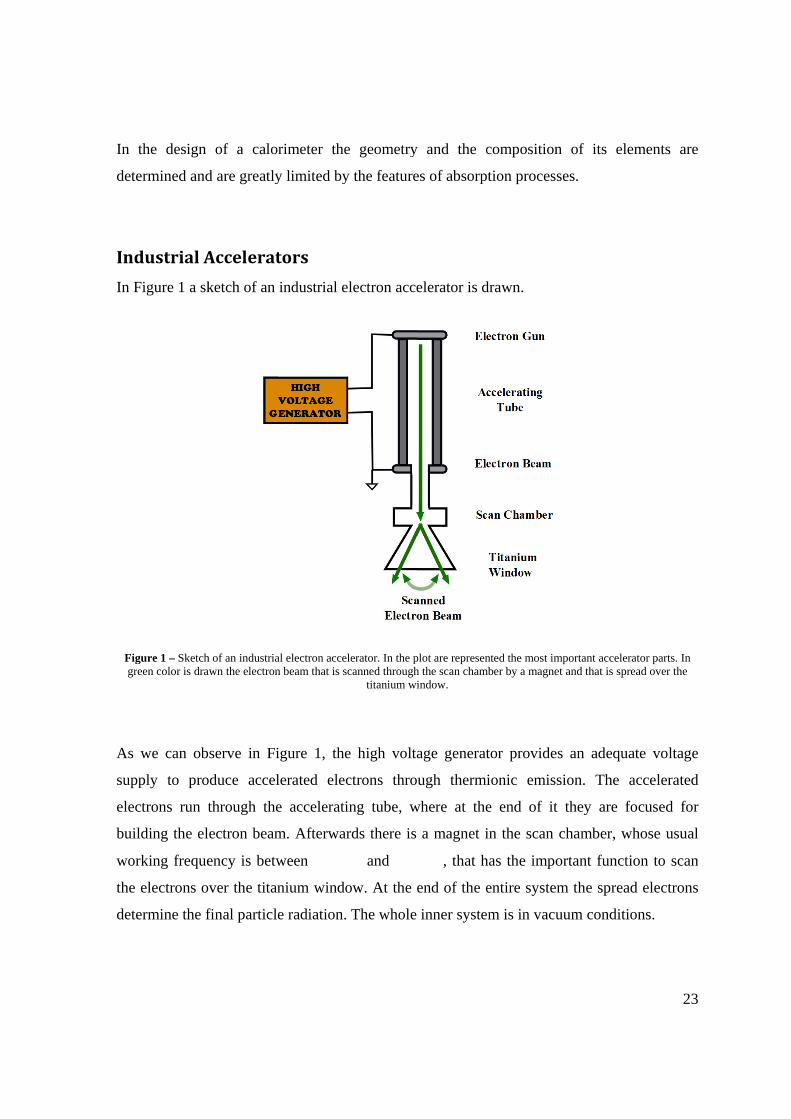
In F
Figgre
As
supp
elec
buil
wor
the
dete
the design
ermined and
dustrial A
Figure 1 a sk
gure 1 – Sketcheen color is dra
we can ob
ply to pro
ctrons run t
lding the el
rking freque
electrons o
ermine the f
of a calor
d are greatly
Accelerat
ketch of an
h of an industriaawn the electron
serve in Fi
oduce accel
through the
ectron beam
ency is betw
ver the titan
final particle
rimeter the
y limited by
tors
industrial e
al electron acceln beam that is sc
igure 1, the
lerated elec
e accelerati
m. Afterwar
ween
nium windo
e radiation.
e geometry
y the feature
electron acce
lerator. In the pcanned through
titanium wi
e high volta
ctrons thro
ing tube, w
rds there is
and
ow. At the e
The whole
y and the c
es of absorp
elerator is d
plot are represenh the scan chamindow.
age generat
ugh thermi
where at the
a magnet i
, that h
end of the e
inner syste
composition
ption proces
drawn.
nted the most immber by a magne
tor provide
ionic emis
e end of it
in the scan
has the impo
entire syste
em is in vacu
n of its el
ses.
mportant acceleet and that is sp
es an adequ
sion. The
t they are f
chamber, w
ortant funct
m the sprea
uum condit
23
lements are
erator parts. In pread over the
uate voltage
accelerated
focused for
whose usual
tion to scan
ad electrons
ions.
3
e
e
d
r
l
n
s
24
The accelerator we deal with has a 40 titanium scanner window and the scanning area is
120 4.5 540 . During the crossliking processes cables pass under the electron
beam at a speed of several / , while our calorimeter will be passing under the accelerator
window at about 18 distance, set on a conveyor with a constant speed of 3.3 , that is
5.5 .
Simulation Tool: ANSYS Workbench 12.1
Engineers routinely use Solid Modelers together with the Finite Element Method (FEM) to
solve everyday problems of modeling for form/fit/function, stress deformation, heat transfer,
fluid flow, electromagnetic, etc. using commercial as well as special purpose software.
ANSYS Workbench is one of the most versatile and widely used of the commercial solid
modeling, simulation and optimization programs, as we can see in [1].
Finite element analysis, on which ANSYS WB is based on, is a computer-based numerical
technique that is used to solve stress analysis, heat transfer, fluid flow and other types of
engineering problems. It is based on solving a system of equations that describe some
parameters over the domain of a continuous physical system. The real power of the finite
element method lies in its ability of analyzing physical parts that are of any shape or size
having arbitrarily located loads and supports.
As the name implies, finite element analysis involves the partitioning (also called
discretizing) of a structure into a finite number of elements. Elements are connected to one
another at their corner points. These corner points are called nodes or nodal points. Each
element is a simple geometric shape, such as a triangle or a quadrilateral. Being a standard
shape (triangle, quadrilateral) facilitate the development of the governing equations that
relate to displacement and stress behavior within the element.
In order to completely determine a finite element model, nodal points, elements, loads,
supports and element related data (such as material properties) must be defined. Once these
data have been defined, they are submitted to a finite element program for the actual
computational process. The program then formulates a set of simultaneous equations, which

25
are the equilibrium equations corresponding to each degree of freedom (directions in which
movement can occur) at each nodal point. A nodal point can have up to six degrees of
freedom – translation in the x, y and z directions and rotation about each of these axes.
In ANSYS WB there are a lot of useful applications, but, as the use of this software has the
aim to perform thermal simulations, only the Design Modeler – to sketch the geometric
model – and the Mechanical Simulation – which performs the thermal simulation – are
relevant functions for the considered system.
Thermal Analysis in ANSYS Workbench
A thermal analysis calculates the temperature distribution and related thermal quantities in a
system or component. Typical thermal quantities of interest are:
• Temperature distributions;
• Amount of lost or gained heat;
• Thermal gradients;
• Thermal fluxes.
The first step in setting a thermal analysis is to understand whether the simulation loads vary
over time or not. If the imposed magnitudes are kept constant, the analysis that should be
selected is the steady-state one; otherwise the transient thermal is needed. ANSYS WB
supports both steady-state and transient analyses, which are briefly described in the following
paragraphs. We have to specify that the first approach towards the resolution of the thermal
problem has been of steady-state type. But, to give the simulations a more realistic view and
to reproduce the physical aspects of the electron beam (source of irradiation in the
experiment), the final run simulations are of transient thermal type. In the end we need
transient thermal simulations, as the calorimeter does not have a fixed position, in facts it is
moved past the electron beam window by a conveyor, so that we can think that the
calorimeter moves with a constant speed (3.3 or 5.5 ).
26
SteadyState Thermal Analysis
A steady-state thermal analysis calculates the effects of steady thermal loads on a system or
on a component. Engineers and analysts often perform a steady-state analysis before doing a
transient thermal one, to help establish initial conditions.
A steady-state thermal analysis can be used to determine temperatures, thermal gradients,
heat flow rates and heat fluxes in an object. All these properties are caused by thermal loads
that do not vary over time. Such loads include the following:
• Convection;
• Radiation
• Heat flow rate;
• Heat flux (heat flow per unit area);
• Heat generation rate (heat flow per unit volume).
A steady-state thermal analysis may be either linear, with constant material properties, or
nonlinear, with material properties that depend on temperature.
Transient Thermal Analysis
A transient thermal analysis determines temperatures and other significant thermal quantities
that vary over time. Engineers commonly use temperatures that a transient thermal analysis
calculates, as input to structural analyses for thermal stress evaluations.
A transient thermal analysis basically follows the same procedures as a steady-state one. The
main difference is that the applied loads are functions of time.
In ANSYS Workbench to specify time-dependent loads, we have to enter the number of steps
in the “Analysis Settings” menu and we have to write the duration of each step in the
respective “Tabular Data”. Afterwards we need to attribute the correct load values to each
step.
27
Novelty of the Approach
As defined in [5], the calorimetric method, which is analyzed in this work, is a quasi-
adiabatic system. By thermodynamic definition, an object is in adiabatic equilibrium if there
is no net heat exchange with its environment. In principle a situation whereby there is no net
heat exchange can be achieved if the temperatures of the object and its surroundings are in
equilibrium all the time. In our case the absorber is at first heated more than the surrounding
envelope, so that we can talk about a quasi-adiabatic system, where the heat losses are
reduced as much as possible thanks to the insulation layers.
The standard approach towards radiation dosimetry through calorimetry is to measure the
superficial dose with a very thin absorber, as previously explained. This goal can be
achieved, because the normalized deposed dose shape is represented by a known fit curve,
driven by experimental data. This experimental curve is the starting point for standard
calorimetry, through which the radiation characteristics can be reconstructed. Indeed, when
the superficial dose has been achieved, i.e. the value that can be set as initial value of the
normalized absorbed dose, the most relevant characteristics of interaction between matter and
radiation driven by the fit curve are known. Instead of using the traditional method of the
fitting curve, we use EBXLINK 1D/3D Monte Carlo simulator, which means that we impose
the general characteristics of the radiation system, such as the geometry and material
properties, so that we get the right information concerning the absorbed dose by matter.
Our approach is different from the usual one, as our key aim is to measure the net average
electron beam energy originated from the accelerator source. Therefore we do not need a thin
calorimeter; on the contrary our method may be called “Integral dose calorimeter”. This
name renders the new idea of our calorimetric system. In fact we need to have information
about the integral absorbed dose curve, which means that we require the area defined by the
absorbed dose curve, i.e. the average dose, so that we can obtain the average electron beam
energy, using equation ( 7 ). Eventually our calorimeter is totally absorbing, meaning that its
thickness is greater than 1 3 of the electron range.
The most evident difference between the standard method and ours consist of the thickness of
the calorimetric body, but also on the new scope, which we deal with. In fact the thicknesses

28
of our absorbers, anticipating what is described in the next chapter, are evaluated considering
a reasonable thickness value, for which the absorbed dose falls to zero (electron range
estimate) – data obtained by simulation of the absorbed dose material that may constitute the
calorimetric body.
In these circumstances we want to establish the energy characteristic of the electron beam
through the temperature rise within the absorber body and the general accelerator behavior
related to the radiation, as we want to provide the accelerator main features.

29
Chapter 2 – Specifications for a new calorimeter
Calorimeter Geometry
At the beginning of the entire problem analysis one of the first questions that has to be
answered consists of the shape of the calorimetric body.
For the choice of the absorber shape, we base our considerations regarding some articles
available in the radiation dosimetry field, such as [3], [6], [7], [8], [9], achieving that the
most used model is defined by a circular shape, so that the absorber is a solid cylinder.
Our problem may be considered one dimensional, in the thickness direction (z axis), because
the most important part of the whole system is the absorbed dose in the third dimension. If
we assume that the calorimeter is wide enough to consider small boundary effects, the two
longitudinal dimensions have only little relevance in the whole subject matter, because of the
integral approach. For this reason we can select the geometry of the absorber without any
constraints concerning the solution itself, but we can choose its shape taking into account
other features for the modeling, such as practical realization and compatibility with the entire
system that has to be built – for instance wires, connections, and temperature sensors.
As one dimension problem, we decide to test the simplest geometrical shapes that can be
constructed: we simulate both the cylinder and the parallelepiped as absorber bodies. There is
no apparent difference between the two shapes, but, as one of the absolute reference
calorimeter is the water one – the water is put in a vessel, usually a Petri dish, whose shape is
round – we settle on modeling a cylinder absorber. Another reason for this choice can be
found in the fact that the circular symmetry is more suitable to a more uniform heat
distribution in reaching the steady-state.
30
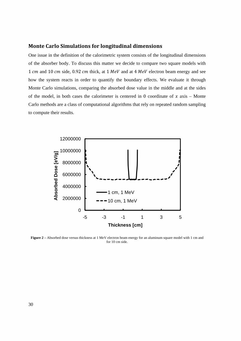
Monte Carlo Simulations for longitudinal dimensions
One issue in the definition of the calorimetric system consists of the longitudinal dimensions
of the absorber body. To discuss this matter we decide to compare two square models with
1 and 10 side, 0.92 thick, at 1 and at 4 electron beam energy and see
how the system reacts in order to quantify the boundary effects. We evaluate it through
Monte Carlo simulations, comparing the absorbed dose value in the middle and at the sides
of the model, in both cases the calorimeter is centered in 0 coordinate of axis – Monte
Carlo methods are a class of computational algorithms that rely on repeated random sampling
to compute their results.
Figure 2 – Absorbed dose versus thickness at 1 MeV electron beam energy for an aluminum square model with 1 cm and for 10 cm side.
0
2000000
4000000
6000000
8000000
10000000
12000000
-5 -3 -1 1 3 5
Abs
orbe
d D
ose
[eV/
g]
Thickness [cm]
1 cm, 1 MeV
10 cm, 1 MeV
31
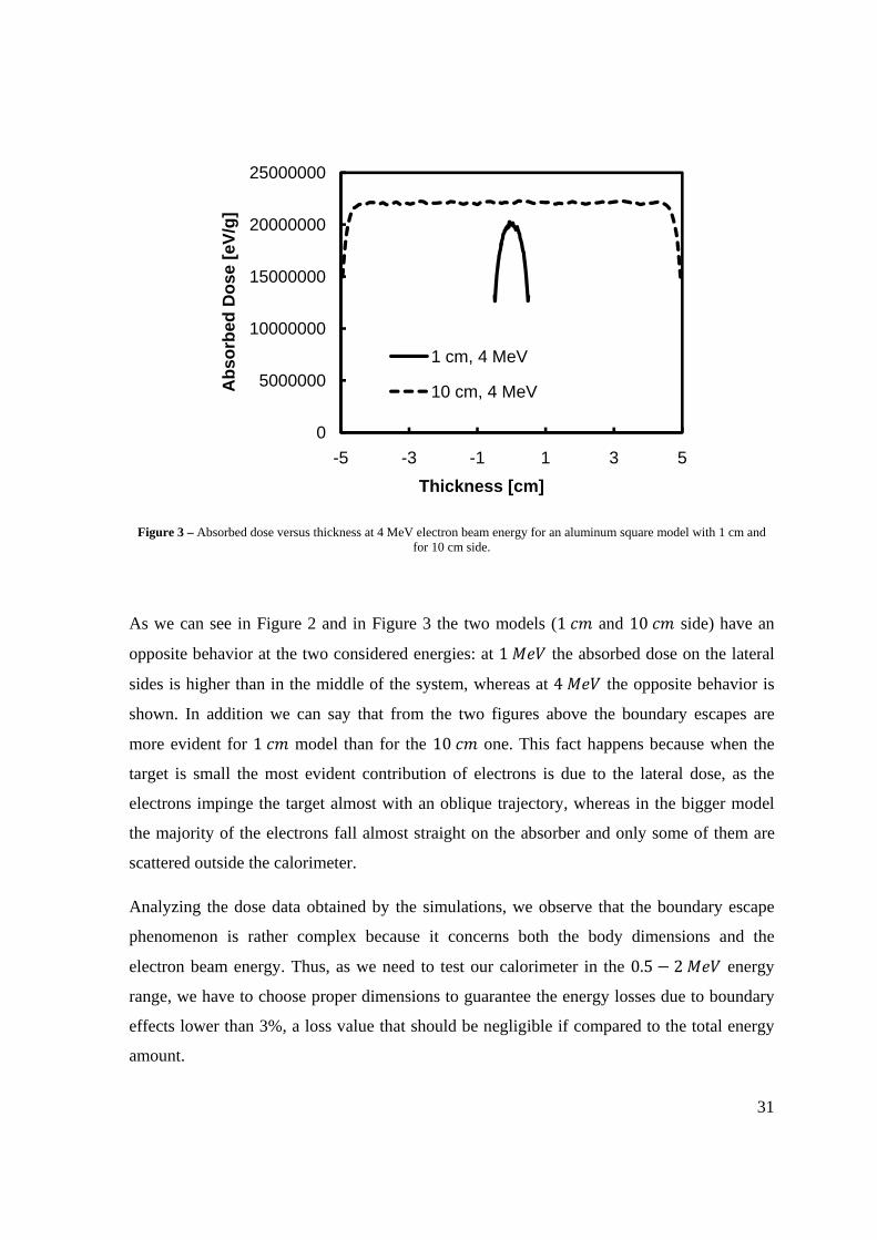
Figure 3 – Absorbed dose versus thickness at 4 MeV electron beam energy for an aluminum square model with 1 cm and for 10 cm side.
As we can see in Figure 2 and in Figure 3 the two models (1 and 10 side) have an
opposite behavior at the two considered energies: at 1 the absorbed dose on the lateral
sides is higher than in the middle of the system, whereas at 4 the opposite behavior is
shown. In addition we can say that from the two figures above the boundary escapes are
more evident for 1 model than for the 10 one. This fact happens because when the
target is small the most evident contribution of electrons is due to the lateral dose, as the
electrons impinge the target almost with an oblique trajectory, whereas in the bigger model
the majority of the electrons fall almost straight on the absorber and only some of them are
scattered outside the calorimeter.
Analyzing the dose data obtained by the simulations, we observe that the boundary escape
phenomenon is rather complex because it concerns both the body dimensions and the
electron beam energy. Thus, as we need to test our calorimeter in the 0.5 2 energy
range, we have to choose proper dimensions to guarantee the energy losses due to boundary
effects lower than 3%, a loss value that should be negligible if compared to the total energy
amount.
0
5000000
10000000
15000000
20000000
25000000
-5 -3 -1 1 3 5
Abs
orbe
d D
ose
[eV/
g]
Thickness [cm]
1 cm, 4 MeV
10 cm, 4 MeV
32
Thereby we opt for a cylinder model with 9 diameter, to render the boundary escapes as
small as possible.
Absorber Materials
Even though any material could be selected as calorimetric absorber, we find out that the
most used materials are: water, polystyrene and graphite – as we can see in several
references: [3], [4], [6], [7], [8], [9], [10], [11].
In [3] are described the calorimeters used for industrial electron accelerators: they are
constructed in graphite, polystyrene or with a Petri dish filled with water as calorimetric
body. In addition polymeric materials other than polystyrene may be used for calorimetric
measurements, but polystyrene is usually chosen because it is known to be resistant to
radiation and because no exo- or endothermic reactions take place.
The typical water, graphite, and polystyrene calorimeter equipments, illustrated in [3], have
similar features. Both the graphite and the polystyrene calorimeters are composed of a disc
placed in a thermally-insulating material such as foamed plastic. A calibrated thermistor or
thermocouple is embedded inside the disc. A water calorimeter is a sealed polystyrene Petri
dish filled with water and placed in thermally-insulating foamed plastic. A calibrated
temperature sensor (thermistor) is placed through the side of the dish into the water.
At first we leave the water calorimeter aside – since the water absorber is the reference model
because it has the most well-known and stable – and we decide to test through Ansys WB
simulator five different materials that could constitute the final calorimeter absorber. The
chosen elements are: graphite, aluminum, copper, polyethylene, and polystyrene. Among all
the different materials that could have been selected we decide to investigate the just
mentioned materials for the following reasons:
• Graphite (Union Carbide AGOT) [4] is used because its irradiation does not lead to
chemical reactions that consume or release significant energy and its atomic number
is comparable to water. Furthermore its thermal diffusivity leads to an even
distribution of heat in the calorimeter absorber, and the graphite is easy to machine;
33
• Aluminum is suggested by [12], as their results agree quite well with simulations;
• Copper is tested because is another metal, like aluminum, that can be easily found and
bought (in this case we want to stress the practical matter of constructing the final
object);
• Polyethylene (PE) is taken into account since it is another polymeric material which
is easily available, above all in the industrial field (for instance cable insulation);
• Polystyrene (PS) is tested because there is plenty available quantities of it and for its
properties described by [3].
Analytical expression
Before approaching the simulative part, it is necessary to have an analytical confirmation of
the temperature difference. The analytical expression we deal with is derived and rearranged
through ( 7 ), where we have to insert the accelerator and calorimeter parameters; the formula
is given by ( 8 ):
Δ · · Δ
· · ·
where Δ is the difference of temperature , is the beam voltage [V], is the beam
current [A], is the irradiated area defined by the scanner , is the calorimeter
thickness , and is the material density .
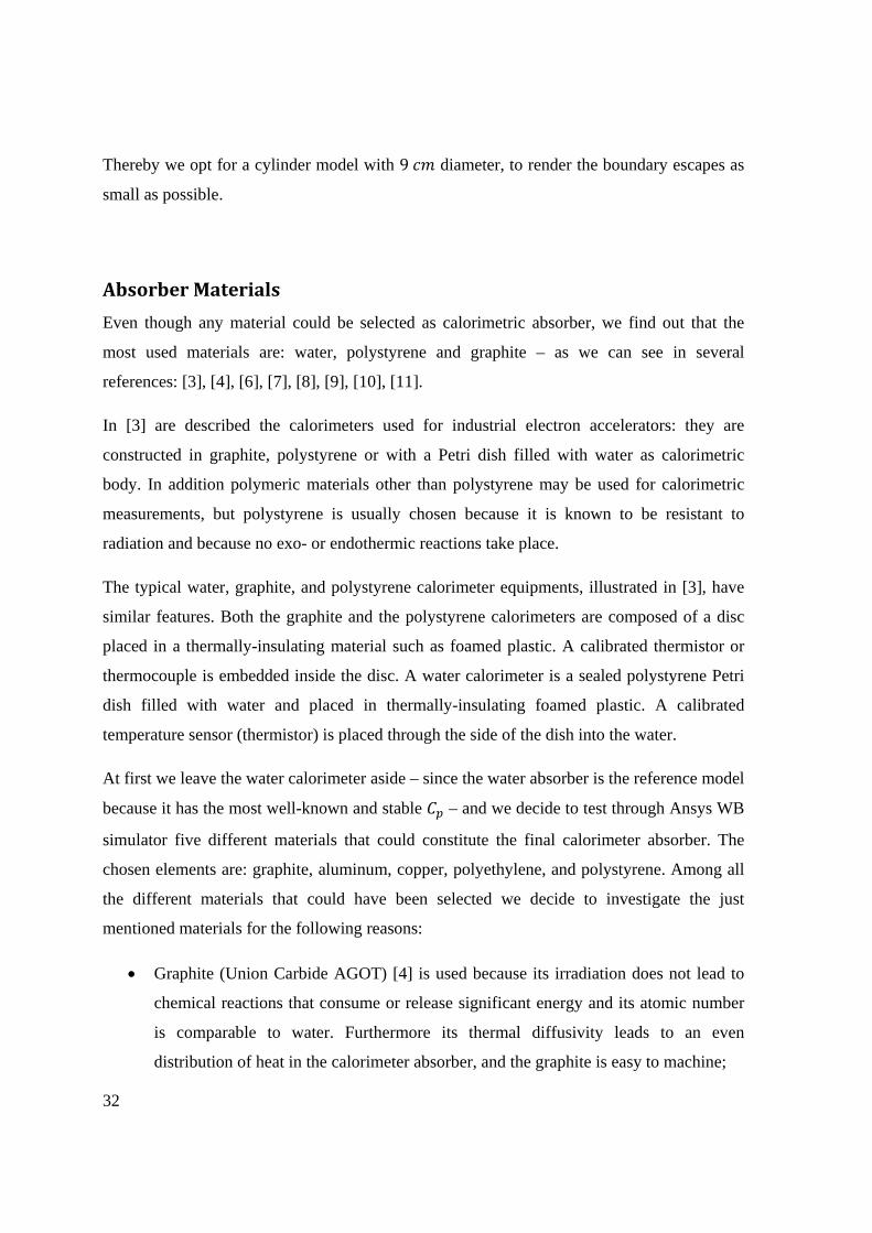
In the next chart of Figure 4 ( 8 ) formula trend is depicted, which stands for the
mathematical mean to estimate the difference of temperature values.
( 8 )
34
Figure 4 – Analytical representation of the reference equation ( 8 ) in logarithmic scale.
As shown in Figure 4 the dependent variable is indeed the difference of temperature, whereas
the independent variable is represented by the product of three parameters that can be set in
the accelerator system: the electron beam voltage, the beam current, and the time due to the
conveyor movement under the accelerator. This graph may be useful if the uncertainties of
the different parameters are not well-known, so that we can establish in a more accurate way
only the final product of the three quantities. The slope of the straight line is defined by the
calorimeter characteristics: irradiated area, specific heat capacity, thickness and density, as
clearly expressed by equation ( 8 ). We set logarithmic axes, because in this way we may
appreciate better the range we deal with. Our working point is namely 1 ,
10 , 0.82 . Thus our x coordinate in Figure 4 is 8.2 · · , to which
corresponds a delta temperature Δ 13.84 .
Thermal Simulations through Ansys WB
At the beginning of the thermal behavior investigation of the above mentioned materials we
focus on a quite large energy range: from 1 to 4 . This energy range does not
0.1
1
10
100
1000
0.1 1 10 100
Del
ta T
empe
ratu
re [K
]
V [MV] · I [mA] · t [s]
Aluminum Calorimeter
35
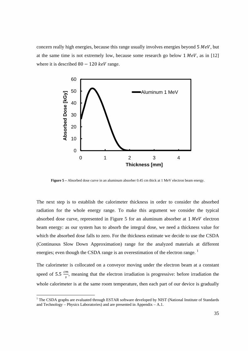
concern really high energies, because this range usually involves energies beyond 5 , but
at the same time is not extremely low, because some research go below 1 , as in [12]
where it is described 80 120 range.
Figure 5 – Absorbed dose curve in an aluminum absorber 0.45 cm thick at 1 MeV electron beam energy.
The next step is to establish the calorimeter thickness in order to consider the absorbed
radiation for the whole energy range. To make this argument we consider the typical
absorbed dose curve, represented in Figure 5 for an aluminum absorber at 1 electron
beam energy: as our system has to absorb the integral dose, we need a thickness value for
which the absorbed dose falls to zero. For the thickness estimate we decide to use the CSDA
(Continuous Slow Down Approximation) range for the analyzed materials at different
energies; even though the CSDA range is an overestimation of the electron range. 1
The calorimeter is collocated on a conveyor moving under the electron beam at a constant
speed of 5.5 , meaning that the electron irradiation is progressive: before irradiation the
whole calorimeter is at the same room temperature, then each part of our device is gradually
1 The CSDA graphs are evaluated through ESTAR software developed by NIST (National Institute of Standards and Technology – Physics Laboratories) and are presented in Appendix – A.1.
0
10
20
30
40
50
60
0 1 2 3 4
Abs
orbe
d D
ose
[kG
y]
Thickness [mm]
Aluminum 1 MeV

36
( 9 )
irradiated (reaching a temperature peak), and at last the calorimeter temperature is equalized
(steady-state). As this process is quite complicated to model, we need to simplify it: we
consider a cylinder calorimeter, whose plot is represented in Figure 6, that is simultaneously
irradiated from the top layer with a uniform electron dose deposition.
Figure 6 – Ansys thermal model: representation of the cylinder calorimeter heating.
When we have to reproduce the electron beam behavior in Ansys WB, there is no application
that may represent the electron transit from the accelerator towards the calorimeter – the
software is used in mechanical branches, where engineers have to simulate physical loads in
a way that involves machines or mechanical engines – so that we have to convert the electron
energy into a heating source. For this reason in Ansys thermal analysis palette we have to
define the “Internal Heat Generation”, but, as the measure unit of this function is , we
have to convert the beam energy to a power per unit volume. Therefore we decide to link the
energy range, the absorber calorimeter thickness, and the heat generation in the following
way: we determine that the calorimeter must have a global thickness of CSDA range at
4 , so that we cover the worst case radiation penetration (upper threshold energy), but, to
characterize the internal heat source, we select a thinner source volume on the absorber,
whose thickness is the CSDA range at 1 (lower threshold energy). Hence we have the
heating source that is represented by the first few millimeters of the calorimeter.
In the conversion from the accelerator energy to the power heating we use the following
expression ( 9 ) (rearranging ( 8 )):

37
··
where is the internal heat source , is the beam voltage , is the beam current ,
is the irradiated area defined by the scanner , and is the source calorimeter
thickness .
For each simulation the starting temperature is set at 22 ° , and, as a consequence of what
has just been explained, for our high energy range analyses, the parameters are set in the
following way:
• 1 ;
• 10 ;
• 540 ;
• is defined for each material by the CSDA range at 1 .
In Figure 7 the internal heat generation, as we need a transient thermal analysis, is shown. It
is the aluminum simulation, and the maximum constant power value is 88.2 . The
duration of the power pulse is 0.82 (the power pulse starts at 1 ) as we have to reproduce
the conveyor movement under the electron beam (before, during, and after radiation phases).
The internal heat radiation for each material is set with the same radiation pulse, where the
power value is related to the considered element through ( 9 ).

38
Figure 7 – Representation of the Internal Heat Generation. It is a power pulse per unit of volume, which duration lasts 0.82s.
This first general analysis is needed to find out the timing properties of the different
materials, so that we can make the best choice not to wait a too long time to reach the steady-
state.
In order to know only the absorber thermal performance, we simulate the calorimetric body
alone, without any envelope, and with perfectly insulated sides, so that every boundary
condition builds an ideal system.
When defining different materials in Ansys, we have to set their properties such as density,
thermal conductivity, and specific heat capacity. Although thermal characteristics such as the
specific heat capacity and the thermal conductivity may vary over temperature, constant
values are assumed to render a simple model and for the temperature range we deal with, we
can assume constant values.
In Table 1 we summarize the material properties we use to simulate our systems.
0102030405060708090
100
0 1 2 3
Inte
rnal
Hae
t Gen
erat
ion
[W/c
m3]
Time [s]
AL Internal Heat Generation

39
Table 1 Material Parameters.
Material CSDA
1MeV
CSDA
4MeV
Specific
Heat
Capacity
Density
Internal
Heat
Generation
Thermal
Conductivity
·
·
Graphite 0.29 1.37 724.28 1.7 63.86 150
Aluminum 0.21 0.92 900 2.7 88.2 237
Copper 0.07 0.31 380 8.96 264.5 401
PE 0.44 2.09 2300 0.94 42.1 0.28
PS 0.42 1.98 1340 1.06 44.1 0.15
Through the data gathered in Table 1, we present the simulations run by Ansys. The two
curves shown in each of the following graphs (Figure 8, Figure 9, Figure 10, Figure 11,
Figure 12) depict the average trend of the maximum and minimum temperature in the solid
body, while the heat is distributed over the entire calorimeter in reaching an uniform
equilibrium temperature.
40
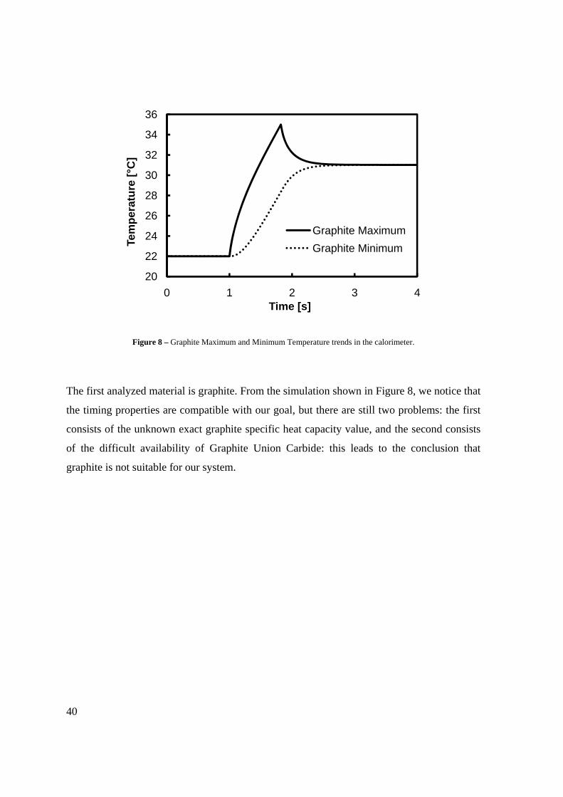
Figure 8 – Graphite Maximum and Minimum Temperature trends in the calorimeter.
The first analyzed material is graphite. From the simulation shown in Figure 8, we notice that
the timing properties are compatible with our goal, but there are still two problems: the first
consists of the unknown exact graphite specific heat capacity value, and the second consists
of the difficult availability of Graphite Union Carbide: this leads to the conclusion that
graphite is not suitable for our system.
20
22
24
26
28
30
32
34
36
0 1 2 3 4
Tem
pera
ture
[°C
]
Time [s]
Graphite MaximumGraphite Minimum

41
Figure 9 – Aluminum Maximum and Minimum Temperature trends in the calorimeter.
In Figure 9 the aluminum temperature trends are represented. We observe that this material
reaches the steady state quickly, so that it may be our candidate for the calorimetric system.
Aluminum has a reaction behavior very close to graphite, but it easier to find and buy.
Figure 10 – Copper Maximum and Minimum Temperature trends in the calorimeter.
20
22
24
26
28
30
32
0 1 2 3
Tem
pera
ture
[°C
]
Time [s]
Aluminum MaximumAluminum Mininum
20222426283032343638
0 0.5 1 1.5 2
Tem
pera
ture
[°C
]
Time [s]
Copper MaximumCopper Mininum

42
In Figure 10 the copper simulation is plotted. Also this metal has a very rapid time reaction;
the only fact that prevents us going further with this model is that copper is a material with
quite a high atomic number (heavy element), so that there could be some problems
concerning x-ray emissions.
In Figure 11 and Figure 12 the polyethylene (PE) and polystyrene (PS) simulations are
shown. We can notice that in both cases the simulations have to run for a very long time
(3500 ) and that there is an anomalous non physical behavior just after the power pulse,
probably due to the numerical analysis and maybe to the high thermal resistivity value.
Figure 11 – Polyethylene (PE) Maximum and Minimum Temperature trends in the calorimeter.
20
25
30
35
40
45
0 1000 2000 3000
Tem
pera
ture
[°C
]
Time [s]
PE MaximumPE Minimum

43
Figure 12 – Polystyrene (PS) Maximum and Minimum Temperature trends in the calorimeter.
Thanks to the previous analyses we discover that these polymers are not consistent for our
purpose, because of the extremely long time constants. In fact if the materials had a too long
time constant, they would cool down before reaching the steady-state, completely altering the
temperature measurement.
In Table 2 all the data from the former graphs are collected.
20
25
30
35
40
45
50
55
0 1000 2000 3000
Tem
pera
ture
[°C
]
Time [s]
PS MaximumPS Minimum
44
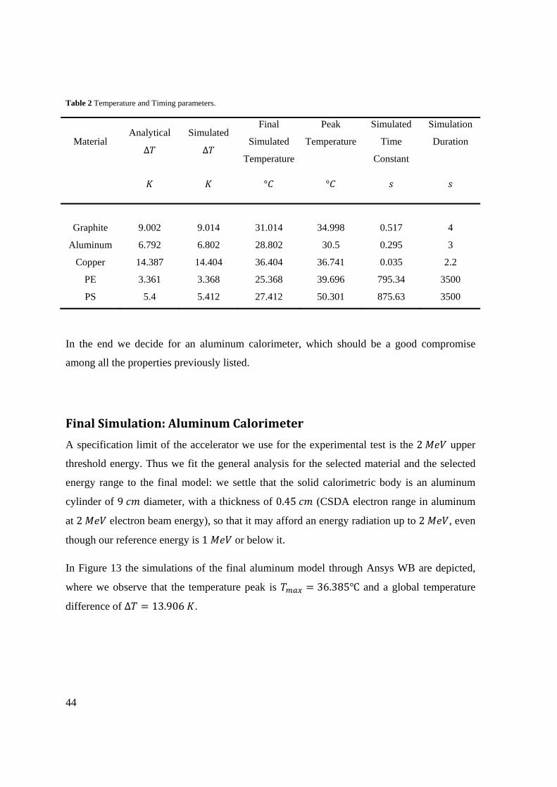
Table 2 Temperature and Timing parameters.
Material Analytical
Δ
Simulated
Δ
Final
Simulated
Temperature
Peak
Temperature
Simulated
Time
Constant
Simulation
Duration
° °
Graphite 9.002 9.014 31.014 34.998 0.517 4
Aluminum 6.792 6.802 28.802 30.5 0.295 3
Copper 14.387 14.404 36.404 36.741 0.035 2.2
PE 3.361 3.368 25.368 39.696 795.34 3500
PS 5.4 5.412 27.412 50.301 875.63 3500
In the end we decide for an aluminum calorimeter, which should be a good compromise
among all the properties previously listed.
Final Simulation: Aluminum Calorimeter
A specification limit of the accelerator we use for the experimental test is the 2 upper
threshold energy. Thus we fit the general analysis for the selected material and the selected
energy range to the final model: we settle that the solid calorimetric body is an aluminum
cylinder of 9 diameter, with a thickness of 0.45 (CSDA electron range in aluminum
at 2 electron beam energy), so that it may afford an energy radiation up to 2 , even
though our reference energy is 1 or below it.
In Figure 13 the simulations of the final aluminum model through Ansys WB are depicted,
where we observe that the temperature peak is 36.385 and a global temperature
difference of Δ 13.906 .

45
Figure 13 – Aluminum Maximum and Minimum Temperature trends in the final model calorimeter.
As we need to proceed as accurately as possible, we measure the final aluminum disc (real
object), obtaining the following dimensions:
• Thickness 0.45 ;
• Diameter 9 ;
• Weight 77.5 .
With these physical dimensions and knowing that the disc has an internal cylindrical hole
(thermal sensor container), whose diameter is 0.16 and length is 3 , we obtain the
density of the material we deal with: 2.71 .
Material Time Constants
Through Ansys analyses we find out the simulated material time constants. After the power
pulse, the temperature decrease does not follow a real exponential curve, so that we cannot
extrapolate the time constant in the usual way. For this reason we consider the difference
20222426283032343638
0 1 2 3
Tem
pera
ture
[°C
]
Time [s]
AL Calorimeter MaxAL Calorimeter Min
46
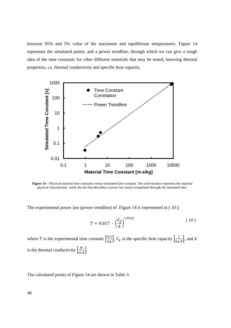
between 95% and 5% value of the maximum and equilibrium temperatures. Figure 14
represents the simulated points, and a power trendline, through which we can give a rough
idea of the time constants for other different materials that may be tested, knowing thermal
properties, i.e. thermal conductivity and specific heat capacity.
Figure 14 – Physical material time constants versus simulated time constant. The solid markers represent the material physical characteristic, while the dot line describes a power law trend extrapolated through the simulated data.
The experimental power law (power trendline) of Figure 14 is represented in ( 10 ):
Τ 0.017 · .
where Τ is the experimental time constant · , is the specific heat capacity ·
, and
is the thermal conductivity ·
.
The calculated points of Figure 14 are shown in Table 3.
( 10 )
0.01
0.1
1
10
100
1000
0.1 1 10 100 1000 10000
Sim
ulat
ed T
ime
Con
stan
t [s]
Material Time Constant [m·s/kg]
Time Constant Correlation
Power Trendline

47
Table 3 Esteemed Timing data.
Material Simul. Time
Constant
·
Graphite 0.517 4.829
Aluminum 0.295 3.797
Copper 0.035 0.948
PE 795.34 8214.3
PS 875.63 8933.3
Through Figure 14 we can remark that the experimental power law is only an estimate of the
real time constant, while comparing the markers and the trendline. We also calculate how big
the error could be, if we relate the power law and the simulated data. Therefore we establish
that the biggest difference is met within copper, with almost 40% error. As previously written
this is not a precise evaluation, since the aim of the trendline is to render a rough estimate of
the material time constant.
Equivalent Compact Thermal Model
As Ansys is a complex simulation tool and our thermal problem is a one-dimensional one, we
examine the thermal analysis as an electrical problem. We determine an electrical compact
equivalent model, shown in Figure 15, where the thermal parameters are converted to
electrical equivalents. This conversion is possible because every thermal parameter has an
electrical equivalent: power becomes current, thermal capacity becomes electrical
capacitance, and thermal resistance becomes electrical resistance. The program used for the
simulations is Spice, whose simple circuit describes the charge distribution of the two
capacitors (they represent the 1 and 4 CSDA thicknesses of Ansys model).
48
Figure 15 – Equivalent compact thermal model.
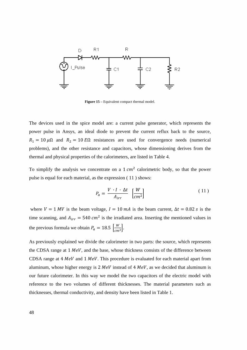
The devices used in the spice model are: a current pulse generator, which represents the
power pulse in Ansys, an ideal diode to prevent the current reflux back to the source,
10 Ω and 10 Ω resistances are used for convergence needs (numerical
problems), and the other resistance and capacitors, whose dimensioning derives from the
thermal and physical properties of the calorimeters, are listed in Table 4.
To simplify the analysis we concentrate on a 1 calorimetric body, so that the power
pulse is equal for each material, as the expression ( 11 ) shows:
· · Δ
where 1 is the beam voltage, 10 is the beam current, Δ 0.82 is the
time scanning, and 540 is the irradiated area. Inserting the mentioned values in
the previous formula we obtain 18.5 .
As previously explained we divide the calorimeter in two parts: the source, which represents
the CDSA range at 1 , and the base, whose thickness consists of the difference between
CDSA range at 4 and 1 . This procedure is evaluated for each material apart from
aluminum, whose higher energy is 2 instead of 4 , as we decided that aluminum is
our future calorimeter. In this way we model the two capacitors of the electric model with
reference to the two volumes of different thicknesses. The material parameters such as
thicknesses, thermal conductivity, and density have been listed in Table 1.
( 11 )

49
Table 4 Electrical circuit parameters.
Material
Ω
Graphite 0.3569 1.3293 0.4567
Aluminum 0.5103 0.5832 0.0949
Copper 0.2383 0.8172 0.0387
PE 0.9513 3.5673 373.21
PS 0.5966 2.2158 660
Equivalent Electrical model: Spice simulations
When simulating the compact model, we can observe that the thermal analysis and the
electrical one correspond with an accuracy of 2% through the following graphs, thus
showing the equivalence of the two methods. The little differences in the temperature values
are shown in Table 5. To simplify the analysis we define the initial temperature at 0 for
each electrical model so that the delta temperature coincides with the steady-state
temperature. We arrange Ansys data removing the initial temperature constant (22 ,) from
the already acquired data and the initial time analysis starting with the power pulse at
0 .
In Figure 16 we report the maximum and the minimum temperature trends of the electrical
circuit representing the aluminum calorimeter. We can notice that the temperature behaviors
are similar to the ones depicted in Figure 13 (Ansys model). The only little differences we
can appreciate are gathered in Table 5 and consist of the maximum peak temperature and of
the steady-state temperature.

50
Figure 16 – Aluminum Maximum and Minimum temperature trends of the electrical circuit.
In Figure 17 we can notice the graphite comparison between the thermal Ansys model and
the compact model. In this case the round marker (Ansys) and the straight line (compact
model) do not match during the first part of the simulation that coincides with the heat pulse.
However the final steady-state temperature is practically the same, as reported in Table 5.
0
2
4
6
8
10
12
14
16
0 0.5 1 1.5 2
Tem
epra
ture
[K]
Time [s]
Max Aluminum Circuit
Min Aluminum Circuit

51
Figure 17 – Graphite comparison between thermal Ansys model and electrical circuit model.
In Figure 18 and Figure 19 are respectively depicted the aluminum and the copper
comparisons (only maximum temperature trends) between thermal Ansys model and
electrical circuit model. From these simulations we see that the round markers (Ansys) and
the straight line (compact model) match almost completely, giving proof of the equivalence
between thermal and electrical models.
0
2
4
6
8
10
12
14
16
0 0.5 1 1.5 2
Tem
epra
ture
[k]
Time [s]
Graphite Circuit
Graphite Ansys

52
Figure 18 – Aluminum comparison between thermal Ansys model and electrical circuit model.
Figure 19 – Copper comparison between thermal Ansys model and electrical circuit model.
0
2
4
6
8
10
12
14
16
0 0.5 1 1.5 2
Tem
epra
ture
[°C
]
Time [s]
Aluminum CircuitAluminum Ansys
0
2
4
6
8
10
12
14
16
0 0.5 1
Tem
epra
ture
[°C
]
Time [s]
Copper Circuit
Copper Ansys
53
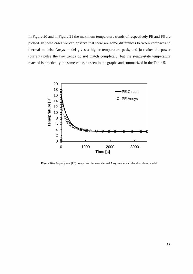
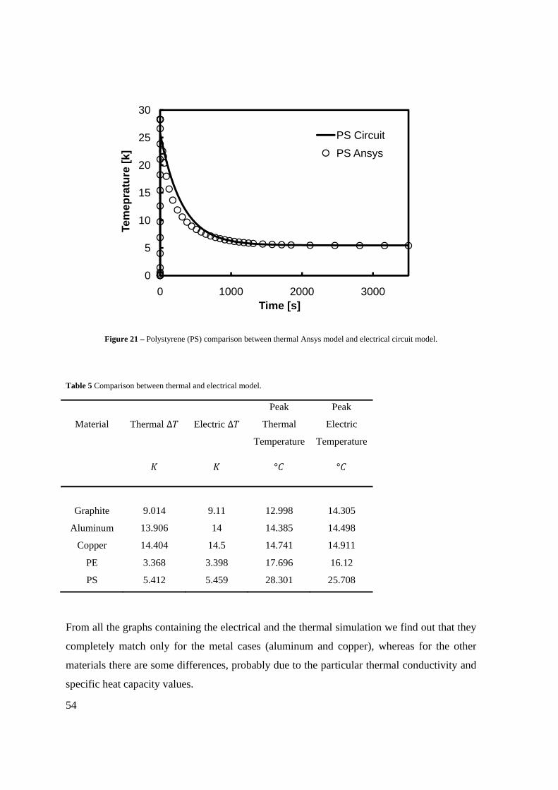
In Figure 20 and in Figure 21 the maximum temperature trends of respectively PE and PS are
plotted. In these cases we can observe that there are some differences between compact and
thermal models: Ansys model gives a higher temperature peak, and just after the power
(current) pulse the two trends do not match completely, but the steady-state temperature
reached is practically the same value, as seen in the graphs and summarized in the Table 5.
Figure 20 – Polyethylene (PE) comparison between thermal Ansys model and electrical circuit model.
02468
101214161820
0 1000 2000 3000
Tem
epra
ture
[K]
Time [s]
PE Circuit
PE Ansys
54
Figure 21 – Polystyrene (PS) comparison between thermal Ansys model and electrical circuit model.
Table 5 Comparison between thermal and electrical model.
Material Thermal Δ Electric Δ
Peak
Thermal
Temperature
Peak
Electric
Temperature
° °
Graphite 9.014 9.11 12.998 14.305
Aluminum 13.906 14 14.385 14.498
Copper 14.404 14.5 14.741 14.911
PE 3.368 3.398 17.696 16.12
PS 5.412 5.459 28.301 25.708
From all the graphs containing the electrical and the thermal simulation we find out that they
completely match only for the metal cases (aluminum and copper), whereas for the other
materials there are some differences, probably due to the particular thermal conductivity and
specific heat capacity values.
0
5
10
15
20
25
30
0 1000 2000 3000
Tem
epra
ture
[k]
Time [s]
PS CircuitPS Ansys

55
Chapter 3 – Hardware Design through Monte Carlo
Simulations
Design Assisted by Dose Simulations: Monte Carlo simulator
After considering the most significant part of the calorimetric system, i.e. the absorber body,
we have to consider the insulator envelope.
A lot of references [3], [4], [6], [8] suggest a complete wrapping up of the calorimetric body
in an insulator box, when analyzing a quite high energy range; whereas the [12] reference,
that deals with a 80 120 energy range, work without complete thermal insulation
because of the short range of electrons. As our energy case is in-between we decide to
examine the entire system with insulation on all sides. From these simulations we have to
establish the envelope dimension.
At first we concentrate on a wide energy range: 1 5 , just to appreciate the differences
in the absorbed dose behavior.
To render the simulation less complicated, we use the following parameters for the
geometrical shapes. The envelope consists of an expanded polystyrene cylindrical box 8
thick with 20 diameter. The expanded polystyrene foam (abbreviation EPS) is considered
with a density 0.03 and a specific heat capacity 1.34 ·
. In the inside
centre there is an aluminum cylinder calorimeter 0.5 thick with 10 diameter.
The following figures represent the simulations evaluated by EBXLIKN 3D Monte Carlo
simulator. These pictures are in three dimensions (3D), because in the x axis it is plotted one
horizontal dimension, in the z axis it is plotted the vertical dimension and the colored scale of
the whole sketch describes the absorbed dose state in the measure unit, which is
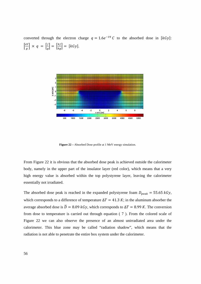
56
converted through the electron charge 1.6 to the absorbed dose in :
.
Figure 22 – Absorbed Dose profile at 1 MeV energy simulation.
From Figure 22 it is obvious that the absorbed dose peak is achieved outside the calorimeter
body, namely in the upper part of the insulator layer (red color), which means that a very
high energy value is absorbed within the top polystyrene layer, leaving the calorimeter
essentially not irradiated.
The absorbed dose peak is reached in the expanded polystyrene foam 55.65 ,
which corresponds to a difference of temperature Δ 41.3 ; in the aluminum absorber the
average absorbed dose is 8.09 , which corresponds to Δ 8.99 . The conversion
from dose to temperature is carried out through equation ( 7 ). From the colored scale of
Figure 22 we can also observe the presence of an almost unirradiated area under the
calorimeter. This blue zone may be called “radiation shadow”, which means that the
radiation is not able to penetrate the entire box system under the calorimeter.

57
Already from Figure 22 we understand that for our purpose and for our reference energy we
cannot have an upper insulation layer, otherwise the absorber is almost not irradiated.
However, to give proof for our assumptions, we analyze and plot in Figure 23 the absorbed
dose in EPS versus the thickness layer. For this reason we run the simulations from 1 to
5 , with 1 step.
Figure 23 – Representation of the Normalized Absorbed Dose trends in the EPS top layer versus its thickness. As the legend shows, we plot the Absorbed Dose percentage at 1 MeV, 2 MeV, 3 MeV, 4 MeV, and 5 MeV electron beam energy to
evaluate the EPS absorption behavior.
If we look at the 1 curve (light blue), we can notice that for the considered thickness,
i.e. 4 , the absorbed dose percentage is almost 45%. This is the reason why we cannot use
a top polymeric layer, like the one we have simulated, because almost half of the incident
radiation is already absorbed in the EPS layer instead of heating the calorimeter, so that we
may not have good measurements.
If on one side the absorbed dose in EPS top layer is very high at 1 energy, on the other
the absorbed dose percentage at 5 (purple curve) is about 6%, that means an acceptable
energy loss, as we can see from the curves presented in Figure 23. This is the reason why,
00.10.20.30.40.50.60.70.80.9
1
1 10 100 1000
% A
bsor
bed
Dos
e
Thickness [mm]
% Abs 1 MeV
% Abs 2 MeV
% Abs 3 MeV
% Abs 4 MeV
% Abs 5 MeV

58
when dealing with high energy ranges, the globally used insulator envelope may be quite
thick, as for instance in [6] reference.
As in Figure 232 (1 beam energy) and later in Figure 26 (5 beam energy) the
Monte Carlo data are presented from a thermal 3D point of view, we convert these data in a
2D graph in Figure 24, where we plot the absorbed dose versus the analyzed thickness, so
that we can compare the absorbed dose profile for the considered threshold energies, i.e.
1 and 5 . We can also observe from the depicted curves in Figure 24 that there is a
big dose gradient at 1 beam energy, due to the major radiation absorption in the upper
expanded polystyrene layer.
Figure 24 – Absorbed Dose profile at 1 MeV and at 5 MeV beam energy.
As a consequence of the absorbed dose curves in Figure 24, we derive the delta temperature
profile in the calorimetric model at 1 and at 5 beam energy, as shown in Figure
25. For the conversion from absorbed dose to temperature we always refer to ( 7 ), where we
have to specify that the temperature profile in EPS is considered punctual because it is an
insulator, whereas the aluminum temperature is constant because the heat distributes in the
whole volume.
0
10
20
30
40
50
60
-5 -3 -1 1 3 5
Abs
orbe
d D
ose
[kG
y]
Thickness [cm]
Dose Profile at 1 MeVDose Profile at 5 MeV
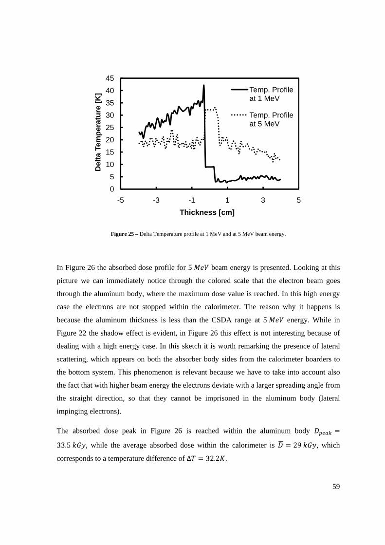
59
Figure 25 – Delta Temperature profile at 1 MeV and at 5 MeV beam energy.
In Figure 26 the absorbed dose profile for 5 beam energy is presented. Looking at this
picture we can immediately notice through the colored scale that the electron beam goes
through the aluminum body, where the maximum dose value is reached. In this high energy
case the electrons are not stopped within the calorimeter. The reason why it happens is
because the aluminum thickness is less than the CSDA range at 5 energy. While in
Figure 22 the shadow effect is evident, in Figure 26 this effect is not interesting because of
dealing with a high energy case. In this sketch it is worth remarking the presence of lateral
scattering, which appears on both the absorber body sides from the calorimeter boarders to
the bottom system. This phenomenon is relevant because we have to take into account also
the fact that with higher beam energy the electrons deviate with a larger spreading angle from
the straight direction, so that they cannot be imprisoned in the aluminum body (lateral
impinging electrons).
The absorbed dose peak in Figure 26 is reached within the aluminum body
33.5 , while the average absorbed dose within the calorimeter is 29 , which
corresponds to a temperature difference of Δ 32.2 .
05
1015202530354045
-5 -3 -1 1 3 5
Del
ta T
empe
ratu
re [K
]
Thickness [cm]
Temp. Profile at 1 MeV
Temp. Profile at 5 MeV
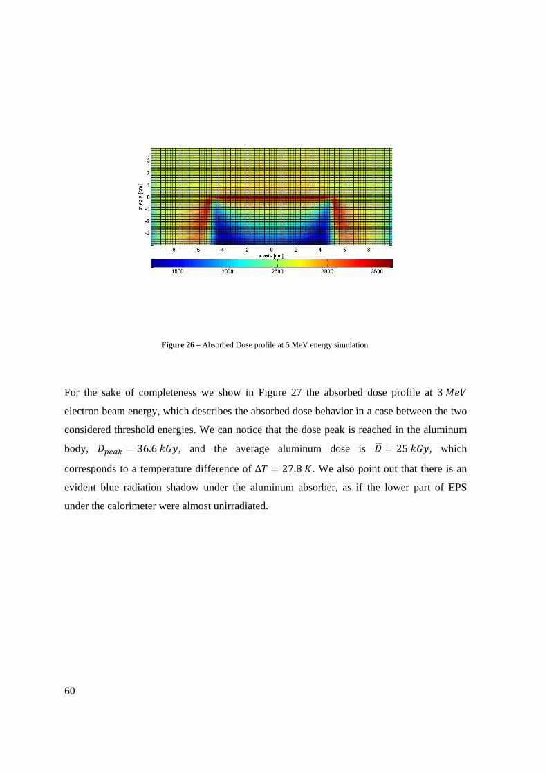
60
Figure 26 – Absorbed Dose profile at 5 MeV energy simulation.
For the sake of completeness we show in Figure 27 the absorbed dose profile at 3
electron beam energy, which describes the absorbed dose behavior in a case between the two
considered threshold energies. We can notice that the dose peak is reached in the aluminum
body, 36.6 , and the average aluminum dose is 25 , which
corresponds to a temperature difference of Δ 27.8 . We also point out that there is an
evident blue radiation shadow under the aluminum absorber, as if the lower part of EPS
under the calorimeter were almost unirradiated.
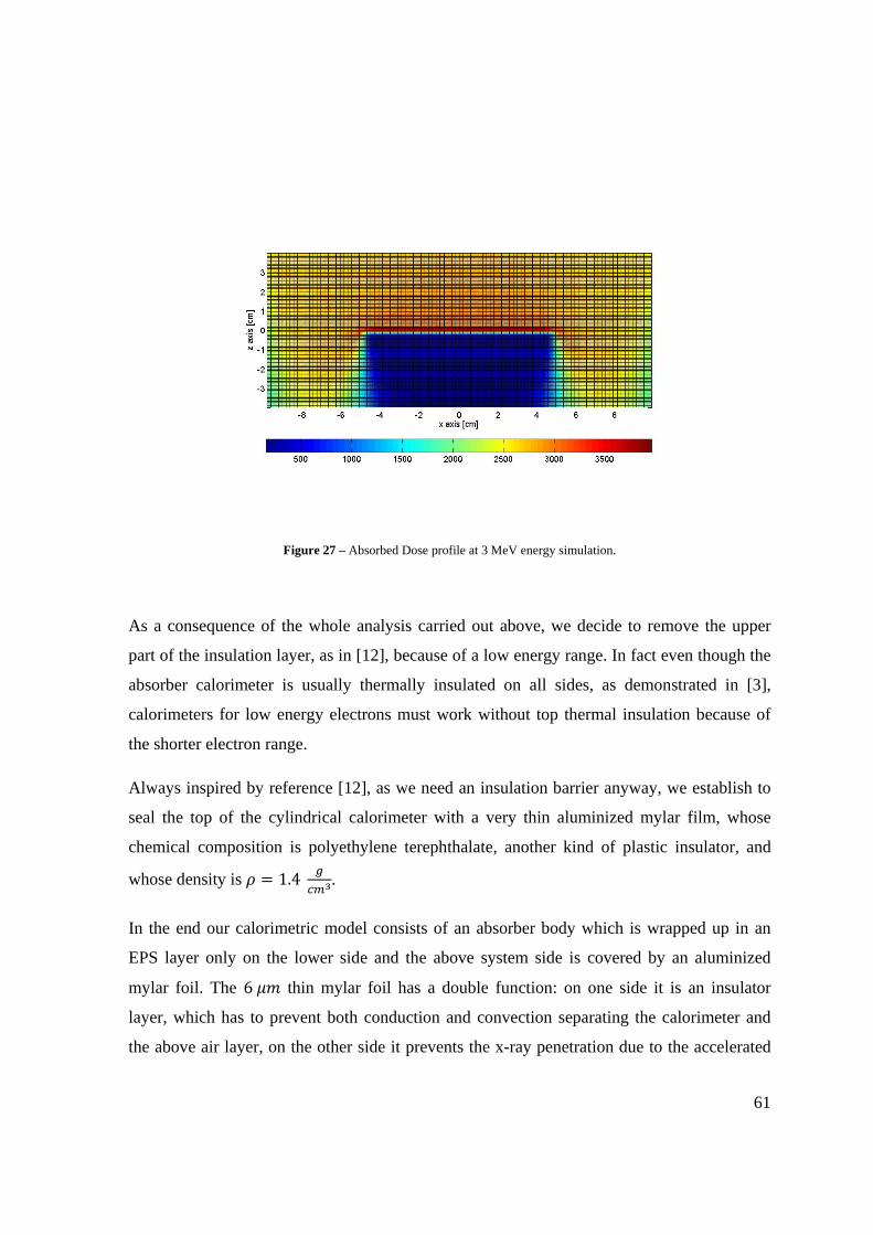
61
Figure 27 – Absorbed Dose profile at 3 MeV energy simulation.
As a consequence of the whole analysis carried out above, we decide to remove the upper
part of the insulation layer, as in [12], because of a low energy range. In fact even though the
absorber calorimeter is usually thermally insulated on all sides, as demonstrated in [3],
calorimeters for low energy electrons must work without top thermal insulation because of
the shorter electron range.
Always inspired by reference [12], as we need an insulation barrier anyway, we establish to
seal the top of the cylindrical calorimeter with a very thin aluminized mylar film, whose
chemical composition is polyethylene terephthalate, another kind of plastic insulator, and
whose density is 1.4 .
In the end our calorimetric model consists of an absorber body which is wrapped up in an
EPS layer only on the lower side and the above system side is covered by an aluminized
mylar foil. The 6 thin mylar foil has a double function: on one side it is an insulator
layer, which has to prevent both conduction and convection separating the calorimeter and
the above air layer, on the other side it prevents the x-ray penetration due to the accelerated
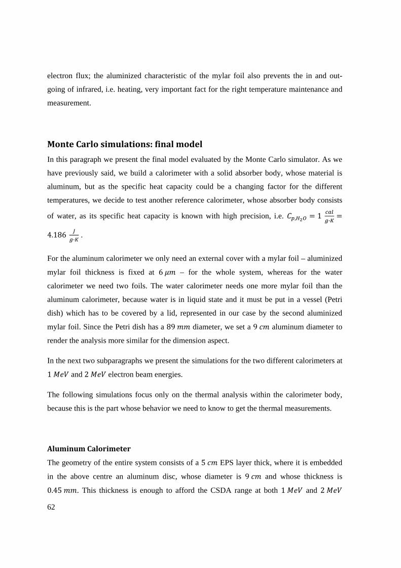
62
electron flux; the aluminized characteristic of the mylar foil also prevents the in and out-
going of infrared, i.e. heating, very important fact for the right temperature maintenance and
measurement.
Monte Carlo simulations: final model
In this paragraph we present the final model evaluated by the Monte Carlo simulator. As we
have previously said, we build a calorimeter with a solid absorber body, whose material is
aluminum, but as the specific heat capacity could be a changing factor for the different
temperatures, we decide to test another reference calorimeter, whose absorber body consists
of water, as its specific heat capacity is known with high precision, i.e. , 1 ·
4.186 ·
.
For the aluminum calorimeter we only need an external cover with a mylar foil – aluminized
mylar foil thickness is fixed at 6 – for the whole system, whereas for the water
calorimeter we need two foils. The water calorimeter needs one more mylar foil than the
aluminum calorimeter, because water is in liquid state and it must be put in a vessel (Petri
dish) which has to be covered by a lid, represented in our case by the second aluminized
mylar foil. Since the Petri dish has a 89 diameter, we set a 9 aluminum diameter to
render the analysis more similar for the dimension aspect.
In the next two subparagraphs we present the simulations for the two different calorimeters at
1 and 2 electron beam energies.
The following simulations focus only on the thermal analysis within the calorimeter body,
because this is the part whose behavior we need to know to get the thermal measurements.
Aluminum Calorimeter
The geometry of the entire system consists of a 5 EPS layer thick, where it is embedded
in the above centre an aluminum disc, whose diameter is 9 and whose thickness is
0.45 . This thickness is enough to afford the CSDA range at both 1 and 2

63
energy – namely the CSDA thickness is 0.21 at 1 and 0.45 at 2 . The
system is covered by a 6 aluminized mylar film.
The following Monte Carlo representations of the absorbed dose focus on the calorimeter
body and its closer layers: at first there is the aluminized mylar foil (6 ), at second the
aluminum calorimeter (0.45 ) and at last the first millimeters of the EPS layer.
Figure 28 – Absorbed dose profile in the aluminum calorimeter at 1 MeV beam energy (3D plot).
From the colored legend we can see that the absorbed dose peak is reached in the first few
millimeters of aluminum. This absorbed dose radiation result is expected, as we model our
system for this purpose, so that there is a dark radiation shadow under the aluminum
calorimeter, as the graph in Figure 28 gives this hint.
On both lateral sides we can see the first parts of the EPS box; their color is yellow, so that
we can understand that this material also absorbs quite a relevant quantity of electrons.
In Figure 29 we extrapolate the dose trend from Monte Carlo data and we remark that the
absorbed dose shape of the curve is the typical one in the Radiation Dosimetry field.
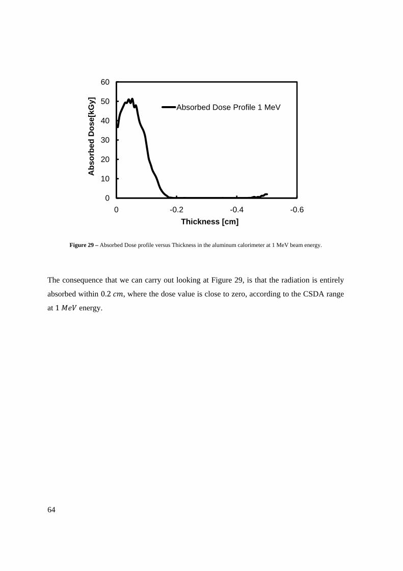
64
Figure 29 – Absorbed Dose profile versus Thickness in the aluminum calorimeter at 1 MeV beam energy.
The consequence that we can carry out looking at Figure 29, is that the radiation is entirely
absorbed within 0.2 , where the dose value is close to zero, according to the CSDA range
at 1 energy.
0
10
20
30
40
50
60
-0.6-0.4-0.20
Abs
orbe
d D
ose[
kGy]
Thickness [cm]
Absorbed Dose Profile 1 MeV

65
Figure 30 – Delta Temperature Profile versus Thickness in the aluminum calorimeter at 1 MeV beam energy.
In Figure 30 we sketch the average temperature in the aluminum body and the punctual
temperature in the first part of expanded polystyrene. We can observe that the average
aluminum temperature is constant, as we assume that the difference of temperature
distributes in the entire cylinder while reaching the steady-state. The difference of
temperature within the absorber is Δ 11.22 .
Now we analyze the 2 energy case.
The graph in Figure 31 shows the absorbed dose profile at 2 beam energy. Also in this
case the dose peak is reached in the first millimeters of the aluminum calorimeter (red color),
but a difference with the previous system is that we observe that the hotter electrons impinge
a thicker layer of aluminum. This is as we expect because of the higher energy and the bigger
CSDA electron range.
0
2
4
6
8
10
12
14
-0.8-0.6-0.4-0.20
Del
ta T
empe
ratu
re [K
]
Thickness [cm]
Temperature Profile 1 MeV

66
Figure 31 – Absorbed dose profile in the aluminum calorimeter at 1 MeV beam energy (3D plot).
In Figure 32 we extrapolate the dose trend from the Monte Carlo data in Figure 31 at 2
electron beam energy.
Figure 32 – Absorbed Dose profile versus Thickness in the aluminum calorimeter at 2 MeV beam energy.
05
101520253035404550
-0.6-0.4-0.20
Abs
orbe
d D
ose[
kGy]
Thickness [cm]
Absorbed Dose Profile 2 MeV
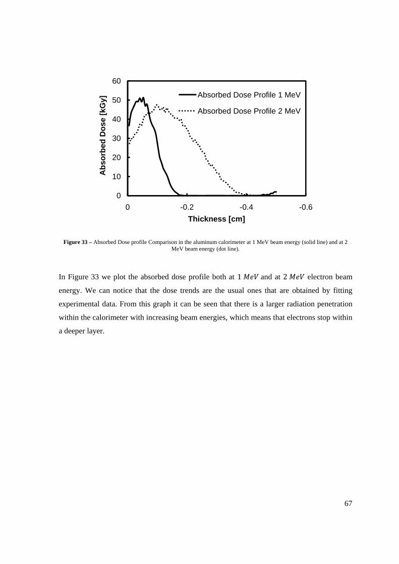
67
Figure 33 – Absorbed Dose profile Comparison in the aluminum calorimeter at 1 MeV beam energy (solid line) and at 2 MeV beam energy (dot line).
In Figure 33 we plot the absorbed dose profile both at 1 and at 2 electron beam
energy. We can notice that the dose trends are the usual ones that are obtained by fitting
experimental data. From this graph it can be seen that there is a larger radiation penetration
within the calorimeter with increasing beam energies, which means that electrons stop within
a deeper layer.
0
10
20
30
40
50
60
-0.6-0.4-0.20
Abs
orbe
d D
ose
[kG
y]
Thickness [cm]
Absorbed Dose Profile 1 MeV
Absorbed Dose Profile 2 MeV
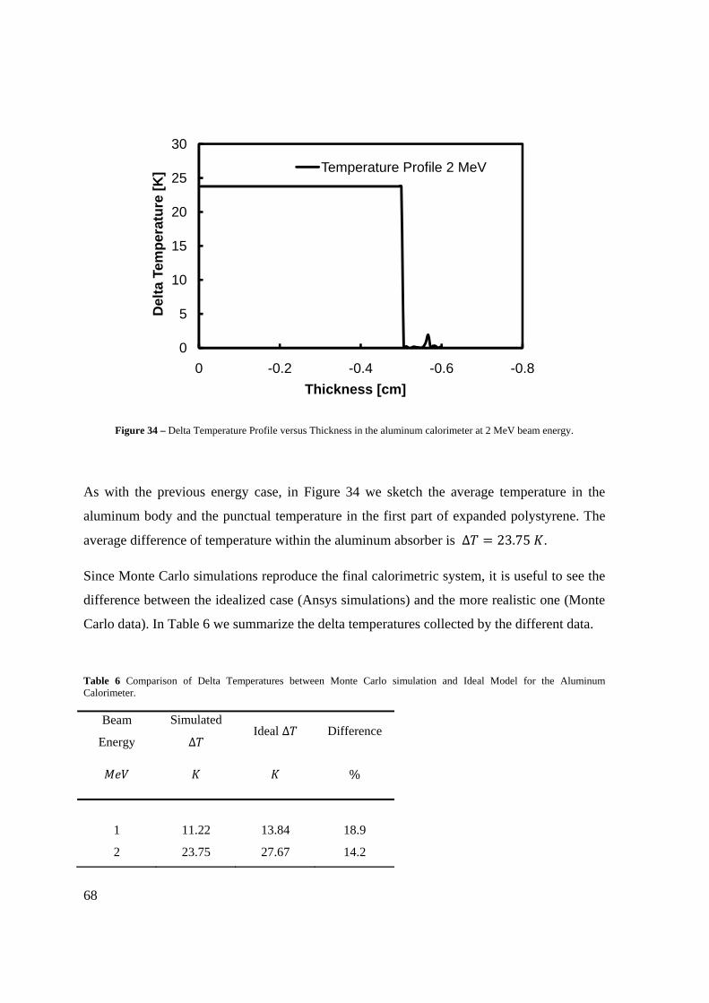
68
Figure 34 – Delta Temperature Profile versus Thickness in the aluminum calorimeter at 2 MeV beam energy.
As with the previous energy case, in Figure 34 we sketch the average temperature in the
aluminum body and the punctual temperature in the first part of expanded polystyrene. The
average difference of temperature within the aluminum absorber is Δ 23.75 .
Since Monte Carlo simulations reproduce the final calorimetric system, it is useful to see the
difference between the idealized case (Ansys simulations) and the more realistic one (Monte
Carlo data). In Table 6 we summarize the delta temperatures collected by the different data.
Table 6 Comparison of Delta Temperatures between Monte Carlo simulation and Ideal Model for the Aluminum Calorimeter.
Beam
Energy
Simulated
Δ Ideal Δ Difference
%
1 11.22 13.84 18.9
2 23.75 27.67 14.2
0
5
10
15
20
25
30
-0.8-0.6-0.4-0.20
Del
ta T
empe
ratu
re [K
]
Thickness [cm]
Temperature Profile 2 MeV

69
We can observe from Table 6 that the estimated Δ difference is higher for the lower energy
case, as the idealized Δ only considers the idealized absorber body, without any other
parameter losses.
Water Calorimeter
The geometry of the water calorimeter consists of a polystyrene Petri dish, 89
diameter, 15.6 thick, and 1.06 density, where the water is collocated with 12
thickness. As with the aluminum calorimeter, the water absorber is embedded on the bottom
part of an EPS layer 5 thick. As already explained we have to put two mylar foils: one
has the same function as in the aluminum calorimeter, i.e. it has to cover and protect the
whole system, while the other mylar foil only covers the Petri dish, so that it works as a lid
for the vessel and as an avoider of water bubbles.
The water thickness is more than enough to afford the CSDA range at both 1 and
2 energy because the computed CSDA ranges are: 0.437 at 1 and 0.9785
at 2 , the real problem in this case is the Petri dish thickness.
Figure 35 – Water calorimeter design with miniature magnetic stirrer. The focus is on the Petri dish, which contains the permanent magnet and water, on the DC motor (1000 rpm), which makes the magnet spin, and on the starter capacitor that
makes the motor drive (rash current).

70
As shown in Figure 35, the real water calorimeter has quite a complicated structure, as it
needs an active forced convection mode for hot and cold water mixing (hot water is due to
electron radiation) and a magnet stirrer that has to spin water for the steady-state temperature
detection. The water calorimeter design has been completed including a dedicated miniature
magnetic stirrer as can be seen in Figure 35.
Figure 36 – Absorbed dose profile in the water calorimeter at 1 MeV beam energy (3D plot).
Through the colored legend of Figure 36 we can see that electrons are totally absorbed within
0.4 thickness, (according to the CSDA range at 1 ); the absorbed dose peak (red) is
reached in the first millimeters of water.
In Figure 37 we extrapolate the absorbed dose profile versus the system thickness through the
data obtained by Figure 36 (Monte Carlo calculations).

71
Figure 37 – Absorbed Dose profile versus Thickness in the water calorimeter at 1 MeV beam energy.
In Figure 38 we sketch the average temperature in the water absorber and the punctual
temperature in the first part of expanded polystyrene. We can observe that the average water
temperature is constant, as we assume that the difference of temperature distributes in the
entire cylindrical vessel to reach the steady-state. The difference of temperature within the
absorber is Δ 2.8 .
0
10
20
30
40
50
60
-1.5-1-0.50
Abs
orbe
d D
ose[
kGy]
Thickness [cm]
Absorbed Dose Profile 1 MeV

72
Figure 38 – Delta Temperature Profile versus Thickness in the aluminum calorimeter at 1 MeV beam energy.
Now we analyze the 2 energy case.
The graph shown in Figure 39 represents the 3D absorbed dose profile in the calorimetric
system at 2 beam energy. Through the color scale we notice that the electrons are
totally absorbed within 0.8 thickness (CSDA range in water at 2 ) , and the absorbed
dose peak (red) is reached in the first millimeters of water.
In Figure 40 we extrapolate the absorbed dose profile versus the system thickness through the
data shown in Figure 39.
0
0.5
1
1.5
2
2.5
3
3.5
-1.5-1-0.50
Del
ta T
empe
ratu
re [K
]
Thickness [cm]
Temperature Profile 1 MeV
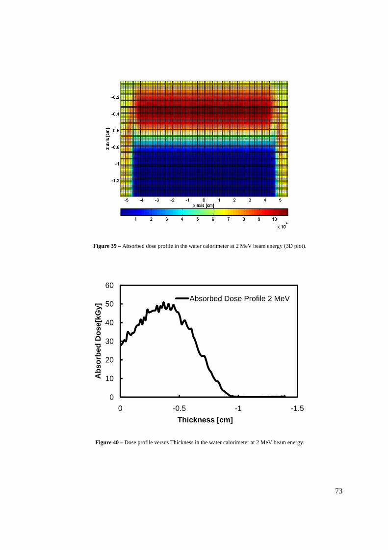
73
Figure 39 – Absorbed dose profile in the water calorimeter at 2 MeV beam energy (3D plot).
Figure 40 – Dose profile versus Thickness in the water calorimeter at 2 MeV beam energy.
0
10
20
30
40
50
60
-1.5-1-0.50
Abs
orbe
d D
ose[
kGy]
Thickness [cm]
Absorbed Dose Profile 2 MeV
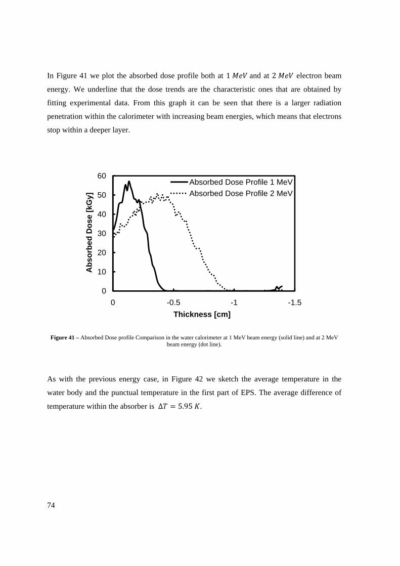
74
In Figure 41 we plot the absorbed dose profile both at 1 and at 2 electron beam
energy. We underline that the dose trends are the characteristic ones that are obtained by
fitting experimental data. From this graph it can be seen that there is a larger radiation
penetration within the calorimeter with increasing beam energies, which means that electrons
stop within a deeper layer.
Figure 41 – Absorbed Dose profile Comparison in the water calorimeter at 1 MeV beam energy (solid line) and at 2 MeV beam energy (dot line).
As with the previous energy case, in Figure 42 we sketch the average temperature in the
water body and the punctual temperature in the first part of EPS. The average difference of
temperature within the absorber is Δ 5.95 .
0
10
20
30
40
50
60
-1.5-1-0.50
Abs
orbe
d D
ose
[kG
y]
Thickness [cm]
Absorbed Dose Profile 1 MeVAbsorbed Dose Profile 2 MeV
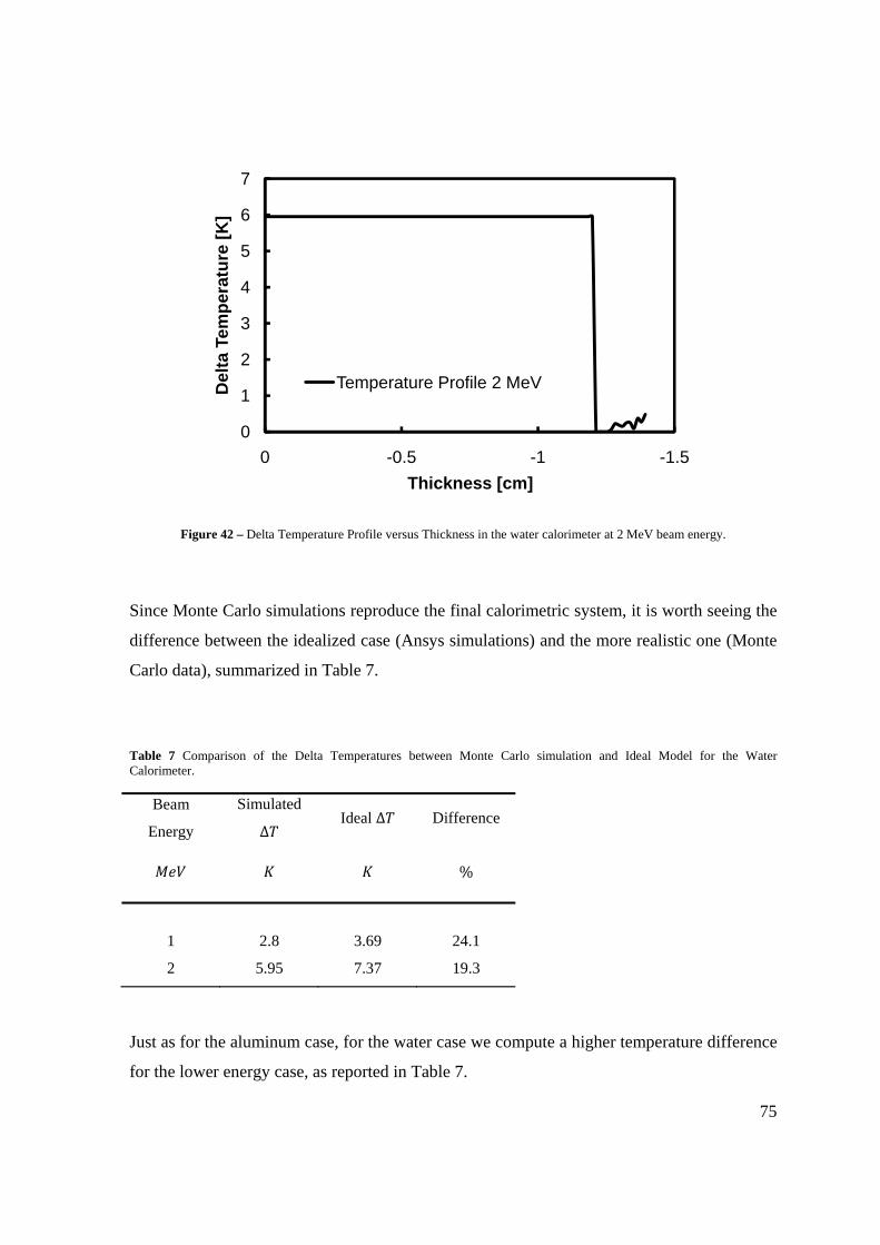
75
Figure 42 – Delta Temperature Profile versus Thickness in the water calorimeter at 2 MeV beam energy.
Since Monte Carlo simulations reproduce the final calorimetric system, it is worth seeing the
difference between the idealized case (Ansys simulations) and the more realistic one (Monte
Carlo data), summarized in Table 7.
Table 7 Comparison of the Delta Temperatures between Monte Carlo simulation and Ideal Model for the Water Calorimeter.
Beam
Energy
Simulated
Δ Ideal Δ Difference
%
1 2.8 3.69 24.1
2 5.95 7.37 19.3
Just as for the aluminum case, for the water case we compute a higher temperature difference
for the lower energy case, as reported in Table 7.
0
1
2
3
4
5
6
7
-1.5-1-0.50
Del
ta T
empe
ratu
re [K
]
Thickness [cm]
Temperature Profile 2 MeV

76

77
Chapter 4 – Global System Design
Hardware design
The global system we physically have to design is composed of an aluminum absorber (9
diameter) and an EPS envelope where the calorimeter is embedded, whose physical model
and exploded view are collected in Figure 43. Since we need to transport our system for the
experimental tests, we need a package (wooden box), which has to include the entire system.
(a) (b)
The wooden box is 29 29 large, it has a 2 thick bottom and a 2 large
lateral edge, so that the internal area results 25 25 . The overall wooden box
thickness is 3 , in order to build a suitable system to let the calorimeter pass under the
Figure 43 – (a) Internal view of the calorimetric system: wooden box expanded polystyrene layers, aluminum cylinder absorber. (b) Exploded view of the integral dose calorimeter.
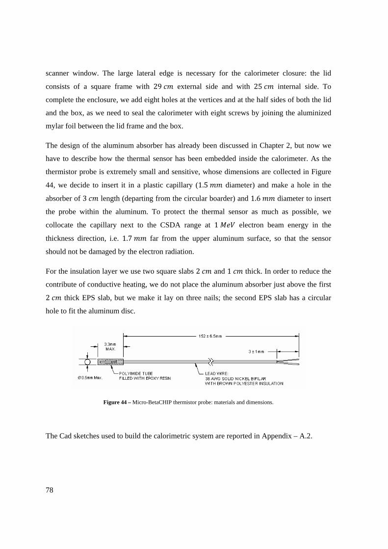
78
scanner window. The large lateral edge is necessary for the calorimeter closure: the lid
consists of a square frame with 29 external side and with 25 internal side. To
complete the enclosure, we add eight holes at the vertices and at the half sides of both the lid
and the box, as we need to seal the calorimeter with eight screws by joining the aluminized
mylar foil between the lid frame and the box.
The design of the aluminum absorber has already been discussed in Chapter 2, but now we
have to describe how the thermal sensor has been embedded inside the calorimeter. As the
thermistor probe is extremely small and sensitive, whose dimensions are collected in Figure
44, we decide to insert it in a plastic capillary (1.5 diameter) and make a hole in the
absorber of 3 length (departing from the circular boarder) and 1.6 diameter to insert
the probe within the aluminum. To protect the thermal sensor as much as possible, we
collocate the capillary next to the CSDA range at 1 electron beam energy in the
thickness direction, i.e. 1.7 far from the upper aluminum surface, so that the sensor
should not be damaged by the electron radiation.
For the insulation layer we use two square slabs 2 and 1 thick. In order to reduce the
contribute of conductive heating, we do not place the aluminum absorber just above the first
2 thick EPS slab, but we make it lay on three nails; the second EPS slab has a circular
hole to fit the aluminum disc.
Figure 44 – Micro-BetaCHIP thermistor probe: materials and dimensions.
The Cad sketches used to build the calorimetric system are reported in Appendix – A.2.

Ins
In t
need
In F
beg
ENE
resi
rem
link
Sign
strument
this paragra
ded during
Figure 45 w
ins with the
ET-9219 th
stance wire
mote control
ked through
nalExpress
tation De
aph we outl
the data col
Figure 45
we sketch a
e Micro-Bet
hrough four
es contribut
(as the calo
h a long Eth
software.
escription
line the cha
llection.
5 – Block diagr
block diagr
taCHIP The
wires for a
te). Finally
orimeter is
hernet cable
n
aracteristics
ram of the elect
ram of the e
ermistor pro
a Kelvin co
y, to acquir
in the accel
e to a PC,
s of the inst
tronic instrumen
entire syste
obe, which i
onfiguration
re the temp
lerator shelt
which is u
trumentatio
ntation connect
m connecti
is connected
n measure (
perature da
ter), the acq
user interfac
on and the c
tions.
ons. The m
d to the dat
in order to
ta through
quisition da
ced through
79
connections
measurement
ta-logger NI
neglect the
a software
ata device is
h LabVIEW
9
s
t
I
e
e
s
W
80
MicroBetaCHIP Thermistor Probe MCD series
The thermal sensor [13] we have chosen is a Micro-BetaCHIP Thermistor, which is a NTC
(Negative Temperature Coefficient) thermistor, whose value at 25 is 10 Ω. From Figure
44 we see the small dimensions of the probe and its construction materials.
We have chosen this sensor for different reasons, that may be found in the device datasheet
[13]: the first is the dimension, as we cannot employ too much space inside the cylinder
absorber (otherwise this term is not negligible compared to the rest mass contribute), the
others are that it has a rapid time constant (200 in liquids), it has a wide temperature
range from 40 to 125 , the guaranteed tolerance is 0.2 from 0 to 70 , and it
has a dissipation constant in air at 25 of 0.3 . In addition the small mass of the unit
allows the sensor to respond very rapidly to temperature changes.
The thermistor measures a resistance value, which has to be converted into a temperature
one: in its datasheet is provided the resistance versus temperature table at 1 step. As during
the measuring process we need a continuous curve to obtain a simultaneous temperature
value, we have to derive an interpolation curve expression, given in equation ( 12 ):
10 · · 273.15
where 0.0053, 0.1196, and 2.8682 are proportional coefficients
established for the resistance to temperature conversion.
The two final extremely thin BetaCHIP wires are connected to an electrical board where the
two wires become four in a flat ribbon cable, as we want to carry out a 4-wires measure
(Kelvin configuration), since it is more accurate than the 2-wires one, because it avoids the
wire-resistance contribute computation.
( 12 )

81
NI ENET9219
Figure 46 – On the left is represented the calorimetric system covered by the aluminized mylar foil. On the right is represented NI ENET-9219 data logger with relative connections.
Our data acquisition instrument is a NI ENET-9219, depicted in Figure 46, by National
Instruments [14], which is an Ethernet 4-channels universal input device that can acquire
several data types. It includes four simultaneously universal measurement channels for
multipurpose testing, such as strain gages, RTDs, thermocouples, load cells, and other power
sensors. In our system, NI ENET-9219 has the function of acquiring data from the Micro-
BetaCHIP thermistor, through which is connected by a flat cable.
From the datasheet characteristics of the DAQ (Data Acquisition acronym) device [14], we
have to point out that the maximum input range of the 4-wires resistance is up to 10.5 Ω, so
that we need a minimum temperature of 24 to reveal any measure, because otherwise the
instrument saturates.
NI ENET-9219 has different methods for data acquisition: high speed (20 ), best 60
rejection (120 ), best 50 rejection (140 ), and high resolution (510 ). For the
resistance measurement the internal peak current provided by the instrument is 500 and,
as we need a quite fast and accurate data collection (we acquire the data during the

82
calorimeter irradiation), we compare the high resolution and high speed ways, considering:
data speed sampling, self heating thermistor, and resolution matters. In the high resolution
acquisition the current pulse is 510 long, while in the high speed it is 20 long. The
main difference lies in a longer current pulse for the high resolution case, whereas in the high
speed case the current pulse is shorter, but it is repeated more frequently to get a faster
measurement. Since we need quite a rapid sampling, we impose to collect one value every
200 , so that we must use the high speed acquisition mode evaluating a 10% duty cycle.
Even for the self heating of the thermistor the high speed mode appears the most suitable
mode, as its duty cycle characterization (10% high speed versus 100% high resolution) lets
us estimate an overheating peak of 8.7 · 10 , while for the high resolution mode it would
be 8.7 , causing intrinsic problems in the calorimeter temperature evaluation. Concerning
the resolution we have tested the instrument with some easy models, carrying out that the
high speed mode has a sufficient resolution for our aim.
The calorimetric system and NI ENET-9219 are located in the accelerator shelter. In order to
prevent electron radiation damage we provide a shielded box where the DAQ system is
assembled, and in order to acquire data through a remote control we provide a 30 Ethernet
cable for the data-logger to PC connection, as the computer is collocated outside the
accelerator shelter.
Remote Control Software: LabVIEW SignalExpress
The software that we use for the data acquisition process is LabVIEW SignalExpress
(National Instruments), which is needed for the project configuration and for the data logger
settings. Through LabVIEW SignalExpress we acquire the resistance value through the
thermistor probe, and the temperature value for the resistance to temperature conversion
using equation ( 12 ). The data logger is finally connected to a computer where we define the
project and where we collect all the temperature data through a 30 Ethernet cable.

83
Figure 47 – LabVIEW SignalExpress screen shoot is divided into three parts: the first panel represents the resistance values acquisition, the second the temperature conversion, and the third is a thermometer for the instantaneous temperature
indication.
In Figure 47 we enclose a LabVIEW SignalExpress screen shoot, where a measure example
is represented. We want to point out the three panels division: the first acquired value is the
resistance one (first black panel), then we convert it into a temperature value through
equation ( 12 ) (second black panel), and in the end we insert a thermometer, which has the
function of revealing the instantaneous Celsius temperature during data acquisition. We have
to underline two details shown in Figure 47: the first is that we can observe that the
calorimeter passes under the electron beam three times, as there are three steps, the second
consists of the negative thermal coefficient of the thermistor, as we can see that if the
resistance value decreases, the temperature value increases. As shown in Figure 47, when the
calorimeter has a higher temperature than its surrounding environment, the thermal sensor
measures a temperature decrease, the cooling slope effect, which must be corrected and
compensated during the data analysis phase.

84
Thermal Sensor Calibration
The Micro-BetaCHIP thermistor probe, as thermal sensor, requires a calibration test, to check
if the temperature we acquire through the thermal sensor inside the calorimeter is the same of
another imposed heat source. To prove this fact, we need an already calibrated instrument as
heating source; the one we use is a “Thermochuck”.
Figure 48 – Calibration curve of the Micro-BetaCHIP thermal sensor. In triangle markers are plotted the experimental data, connected with a straight line (dots).
In Figure 48 we plot the Calibration curve of the Micro-BetaCHIP sensor, which describes
the correlation between the imposed temperature of the heat source and the measured one. As
we can see from Figure 48, the experimental markers (triangle) are perfectly matched in a
straight line (dots), whose expression is 0.9954 0.3339 , and whose minimum
square term is equal to one 1, so that all the data lie on this line. The evaluated slope
0.9954 is almost one and the difference of these two values is less than 1%; we can
explain this behavior taking into account the stochastic tolerance of the probe, whose value is
0.2 . Since the experimental thermistor data match with the heat source, we are able to
assert that the thermistor works in the right temperature range and it does not need any other
calibration or correction factors.
0
20
40
60
80
100
120
20 40 60 80 100 120
Mea
sure
d Te
mpe
ratu
re [°
C]
Imposed Temperature [°C]
Calibration

85
Electron Energy Extrapolation
Basically starting from the measured difference of temperature through the calorimeter we
want to reconstruct the impinging electron energy. To achieve this goal, we write a Matlab
file, attached in Appendix – A.3, in which we rearrange the mathematical expression ( 8 ) to
obtain the interested energy values. Besides the energy values, we estimate the possible error
sources, which are the subject of the following paragraph.
Rearranging equations ( 6 ) and ( 8 ) for 1 area, we obtain ( 13 ).
· · Δ · · · Δ · · Δt
where is the total energy absorbed energy , specific heat capacity ·
, Δ
total difference of temperature , material density , irradiated scanned area
, beam current , Δt scanning time , and beam voltage/electron energy
at the calorimeter surface.
Finally the detected electron energy evaluation (without error corrections) is reported in
equation ( 14 ).
· Δt
· · · · Δ
In the case of the aluminum calorimeter in conjunction with standard measurement
procedures equation ( 14 ) becomes ( 15 ):
722.8 · Δ
Systematic and Random Errors
Every experimental measurement is affected by an inevitable degree of uncertainty, which
does not depend on the accuracy of the measuring method. For this reason, when acquiring
( 13 )
( 14 )
( 15 )
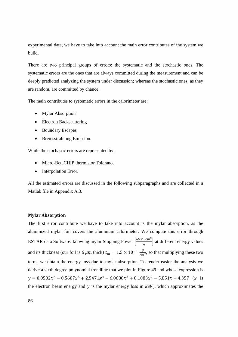
86
experimental data, we have to take into account the main error contributes of the system we
build.
There are two principal groups of errors: the systematic and the stochastic ones. The
systematic errors are the ones that are always committed during the measurement and can be
deeply predicted analyzing the system under discussion; whereas the stochastic ones, as they
are random, are committed by chance.
The main contributes to systematic errors in the calorimeter are:
• Mylar Absorption
• Electron Backscattering
• Boundary Escapes
• Bremsstrahlung Emission.
While the stochastic errors are represented by:
• Micro-BetaCHIP thermistor Tolerance
• Interpolation Error.
All the estimated errors are discussed in the following subparagraphs and are collected in a
Matlab file in Appendix A.3.
Mylar Absorption
The first error contribute we have to take into account is the mylar absorption, as the
aluminized mylar foil covers the aluminum calorimeter. We compute this error through
ESTAR data Software: knowing mylar Stopping Power · at different energy values
and its thickness (our foil is 6 thick) 1.5 10 , so that multiplying these two
terms we obtain the energy loss due to mylar absorption. To render easier the analysis we
derive a sixth degree polynomial trendline that we plot in Figure 49 and whose expression is
0.0502 0.5607 2.5471 6.0688 8.1083 5.851 4.357 ( is
the electron beam energy and is the mylar energy loss in ), which approximates the
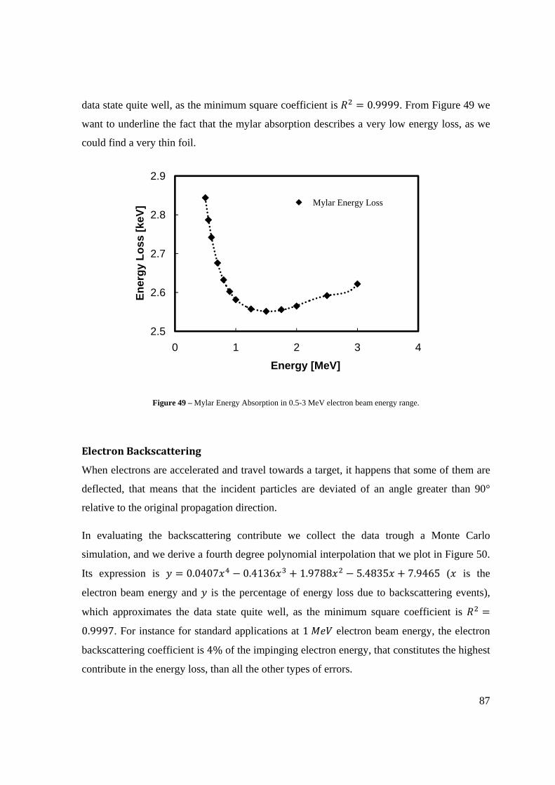
87
data state quite well, as the minimum square coefficient is 0.9999. From Figure 49 we
want to underline the fact that the mylar absorption describes a very low energy loss, as we
could find a very thin foil.
Figure 49 – Mylar Energy Absorption in 0.5-3 MeV electron beam energy range.
Electron Backscattering
When electrons are accelerated and travel towards a target, it happens that some of them are
deflected, that means that the incident particles are deviated of an angle greater than 90°
relative to the original propagation direction.
In evaluating the backscattering contribute we collect the data trough a Monte Carlo
simulation, and we derive a fourth degree polynomial interpolation that we plot in Figure 50.
Its expression is 0.0407 0.4136 1.9788 5.4835 7.9465 ( is the
electron beam energy and is the percentage of energy loss due to backscattering events),
which approximates the data state quite well, as the minimum square coefficient is
0.9997. For instance for standard applications at 1 electron beam energy, the electron
backscattering coefficient is 4% of the impinging electron energy, that constitutes the highest
contribute in the energy loss, than all the other types of errors.
2.5
2.6
2.7
2.8
2.9
0 1 2 3 4
Ener
gy L
oss
[keV
]
Energy [MeV]
Mylar Energy Loss

88
Figure 50 – Percentage Backscattered electrons in 0.5-3 MeV electron beam energy range.
Boundary Escapes
The Boundary Effect consists of electrons that for several reasons do not entirely depose their
dose within the absorber. These particles are mainly: the lateral ones that arrive with an
oblique trajectory and pass through the target releasing only a part of their energy, particles
that may go out of the absorber because of electron path scattering through a mean, and
electrons which impinge the absorber sideways.
11.5
22.5
33.5
44.5
55.5
6
0 1 2 3 4
Bac
ksca
tterin
g %
Energy [MeV]
Aluminum Backscattering

89
Figure 51 – Boundary Effects of the aluminum calorimeter centered in the 0 coordinate of x axis, 9 cm diameter. The y axis represent the normalized absorbed dose.
From the Monte Carlo simulation, whose data are presented in Figure 51, we estimate the
boundary contribute in 1%, computing the difference between the absorbed dose at the
sides and in the middle of the model. As we can see from this figure, the normalized
absorbed dose has a peak on both calorimeter sides, which means that there are more
electrons that enter and depose their energy at the target side, than electrons that go out of it.
For this reason the evaluated boundary contribute has to be subtracted from the acquired
energy value.
Bremsstrahlung Emission (Radiation Yield)
When charged particles are under acceleration it may happen that they emit X-ray radiation
due to different processes that transform electrons in photons sharing energy. This coefficient
is evaluated by ESTAR radiation yield and it is estimated with a 1% energy loss of the
impinging electron energy.
0
0.2
0.4
0.6
0.8
1
1.2
-5 -3 -1 1 3 5
Nor
mal
ized
Abs
orbe
d D
ose
Thickness [cm]
Boundary Effect

90
MicroBetaCHIP Tolerance
Our thermal sensor has a provided tolerance of 0.2 in the temperature reading, value that
has to be counted as a random error for the energy evaluation.
Interpolation Error
The DAQ system acquires resistance data and then converts them into a temperature trend
through equation ( 12 ). The random error that may be committed for the interpolation curve
conversion is estimated in 0.4% of the impinging electron energy from internal
measurements.
91
Chapter 5 – Experimental Results and Discussion
Data Acquisition
When we start with the calorimeter tests, we put it on the conveyor that has the function of
passing under the electron beam with a constant speed of 5.5 . We prove three beam
voltages, namely 0.6 , 0.8 , 1 , and two beam currents, i.e. 5 and 10 .
In the next graphs are shown the acquired temperature trends by the Micro-BetaCHIP sensor
(solid line), and the same data corrected by the initial cooling slope (dots). We may analyze
three or six passages under the accelerator, as we want to test its response (linear, non-linear,
proportional).
From now on we will discuss how the different tests have been conducted and finally we
summarize all the data in Table 8.
In Figure 52, Figure 53, and Figure 54 are collected the tests conducted respectively at 1 ,
0.8 , and 0.6 electron beam voltage nominal values with the same rated beam current
of 10 . For each test we establish three passages and from these figures we can see that
each temperature step has about the same amplitude for each case, but, to render a more
precise analysis, we always take the average value (Δ divided by the number of
passages). In this way we may confront the differences of temperature (in similar boundary
conditions), even though the number of passages of the calorimeter under the scanner may
not be the same.
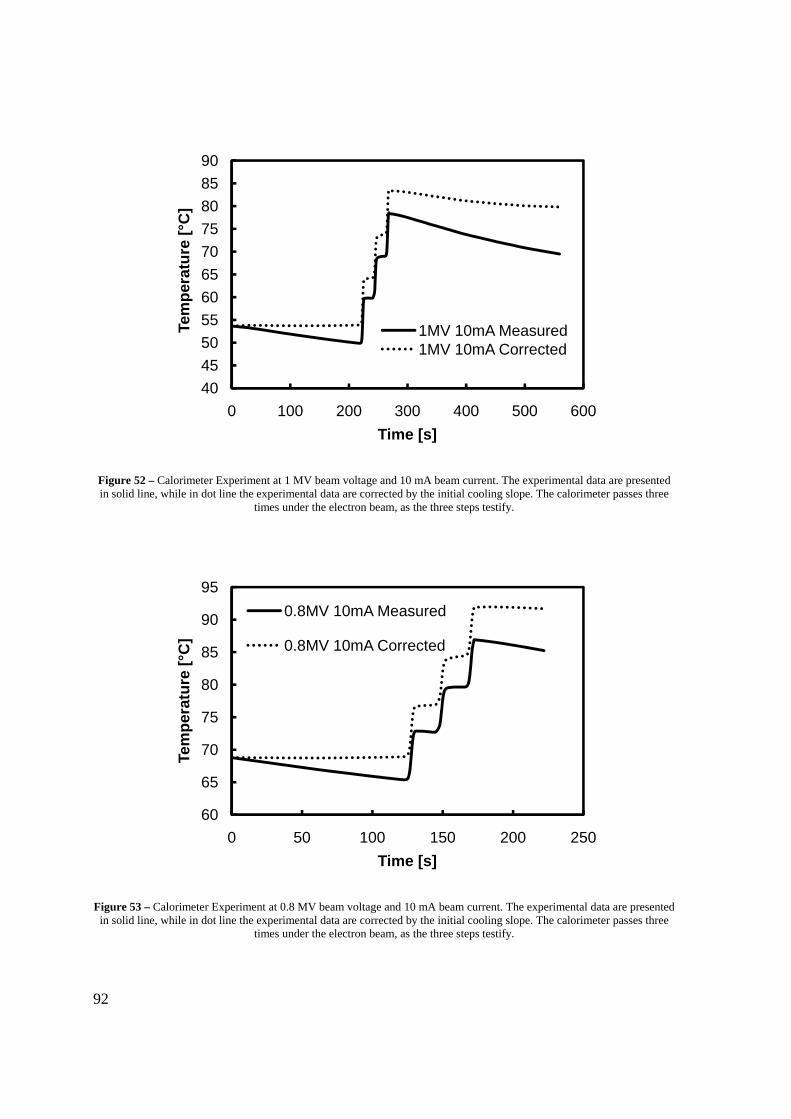
92
Figure 52 – Calorimeter Experiment at 1 MV beam voltage and 10 mA beam current. The experimental data are presented in solid line, while in dot line the experimental data are corrected by the initial cooling slope. The calorimeter passes three
times under the electron beam, as the three steps testify.
Figure 53 – Calorimeter Experiment at 0.8 MV beam voltage and 10 mA beam current. The experimental data are presented in solid line, while in dot line the experimental data are corrected by the initial cooling slope. The calorimeter passes three
times under the electron beam, as the three steps testify.
4045505560657075808590
0 100 200 300 400 500 600
Tem
pera
ture
[°C
]
Time [s]
1MV 10mA Measured1MV 10mA Corrected
60
65
70
75
80
85
90
95
0 50 100 150 200 250
Tem
pera
ture
[°C
]
Time [s]
0.8MV 10mA Measured
0.8MV 10mA Corrected

93
Figure 54 – Calorimeter Experiment at 0.6 MV beam voltage and 10 mA beam current. The experimental data are presented in solid line, while in dot line the experimental data are corrected by the initial cooling slope. The calorimeter passes three
times under the electron beam, as the three steps testify.
In Figure 55, Figure 56, and Figure 57 are reported the tests conducted respectively at 1 ,
0.8 , and 0.6 electron beam voltage nominal values with the same rated beam current
of 5 . Also in this case, in every figure the measured difference of temperature at each
step consists of almost the same value. We remark that for the 1 and 0.6 we have
chosen six passages, while for the 0.8 case we have left three. We underline the fact that
the different number of passages has been tested to prove the accelerator behavior.
60
65
70
75
80
85
90
0 100 200 300
Tem
pera
ture
[°C
]
Time [s]
0.6MV 10mA Measured0.6MV 10mA Corrected
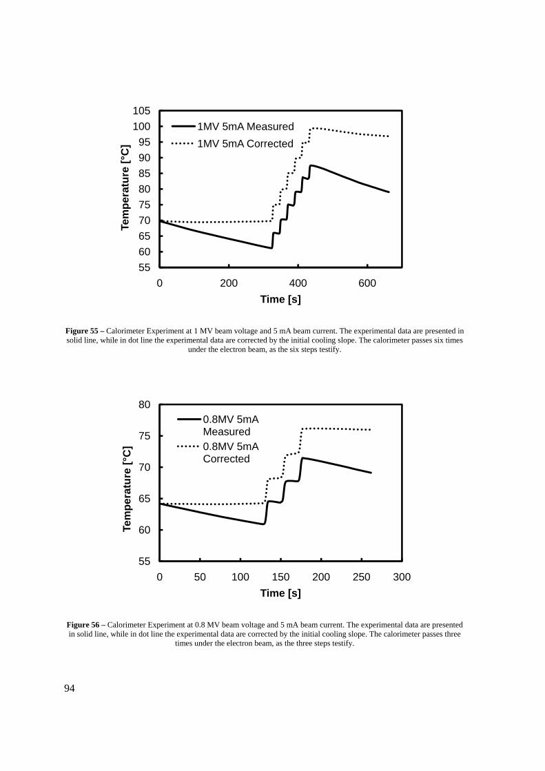
94
Figure 55 – Calorimeter Experiment at 1 MV beam voltage and 5 mA beam current. The experimental data are presented in solid line, while in dot line the experimental data are corrected by the initial cooling slope. The calorimeter passes six times
under the electron beam, as the six steps testify.
Figure 56 – Calorimeter Experiment at 0.8 MV beam voltage and 5 mA beam current. The experimental data are presented in solid line, while in dot line the experimental data are corrected by the initial cooling slope. The calorimeter passes three
times under the electron beam, as the three steps testify.
556065707580859095
100105
0 200 400 600
Tem
pera
ture
[°C
]
Time [s]
1MV 5mA Measured1MV 5mA Corrected
55
60
65
70
75
80
0 50 100 150 200 250 300
Tem
pera
ture
[°C
]
Time [s]
0.8MV 5mA Measured0.8MV 5mA Corrected

95
Figure 57 – Calorimeter Experiment at 0.6 MV beam voltage and 5 mA beam current. The experimental data are presented in solid line, while in dot line the experimental data are corrected by the initial cooling slope. The calorimeter passes six
times under the electron beam, as the six steps testify.
Figure 58 – Calorimeter Experiment at 1 MV beam voltage and 10 mA beam current. The experimental data are presented in solid line, while in dot line the experimental data are corrected by the initial cooling slope. The calorimeter passes once
under the electron beam, as the only step testify.
55
60
65
70
75
80
0 50 100 150 200 250 300
Tem
pera
ture
[°C
]
Time [s]
0.6MV 5mA Measured0.6MV 5mA Corrected
75
80
85
90
95
100
0 100 200 300 400
Tem
pera
ture
[°C
]
Time [s]
1MV 10mA Measured1MV 10mA Corrected

96
In the end we decide to repeat just one passage of the calorimeter under the electron beam, as
shown in Figure 58, to reveal the repeatability of the test. In fact, as Table 8 proves, the
average Δ is very close to the one of the first test with three passages in the same voltage
and current conditions (rated nominal values: 1 , and 10 ).
All the data collected through the experiments and the corrected beam energy values given
by the elaborated Matlab file (Appendix – A.3) are reported in Table 8. The average voltage
and current values of Table 8 are collected by extracting the average term while reading the
nominal voltage/current values provided by the accelerator set up during each conveyor
passage.
Table 8 Calorimeter first batch Experimental Data.
Test
Nominal
Values
Total
Average Δ #
Average
Experimental
Current
Average
Experimental
Voltage
Corrected
Energy
, , #
1, 10, 3 29.65 9.88 10.27 1.0033 735 17
0.8, 10, 3 23.06 7.69 10.33 0.8067 571 16
0.6, 10, 3 15.74 5.25 10.37 0.6067 392 15
1, 5, 6 29.64 4.94 5.18 1.0083 728 31
0.8, 5, 3 11.95 3.98 5.2 0.8067 588 30
0.6, 5, 6 15.55 2.59 5.18 0.6 388 29
1, 10, 1 9.9 9.9 10.6 1 713 16
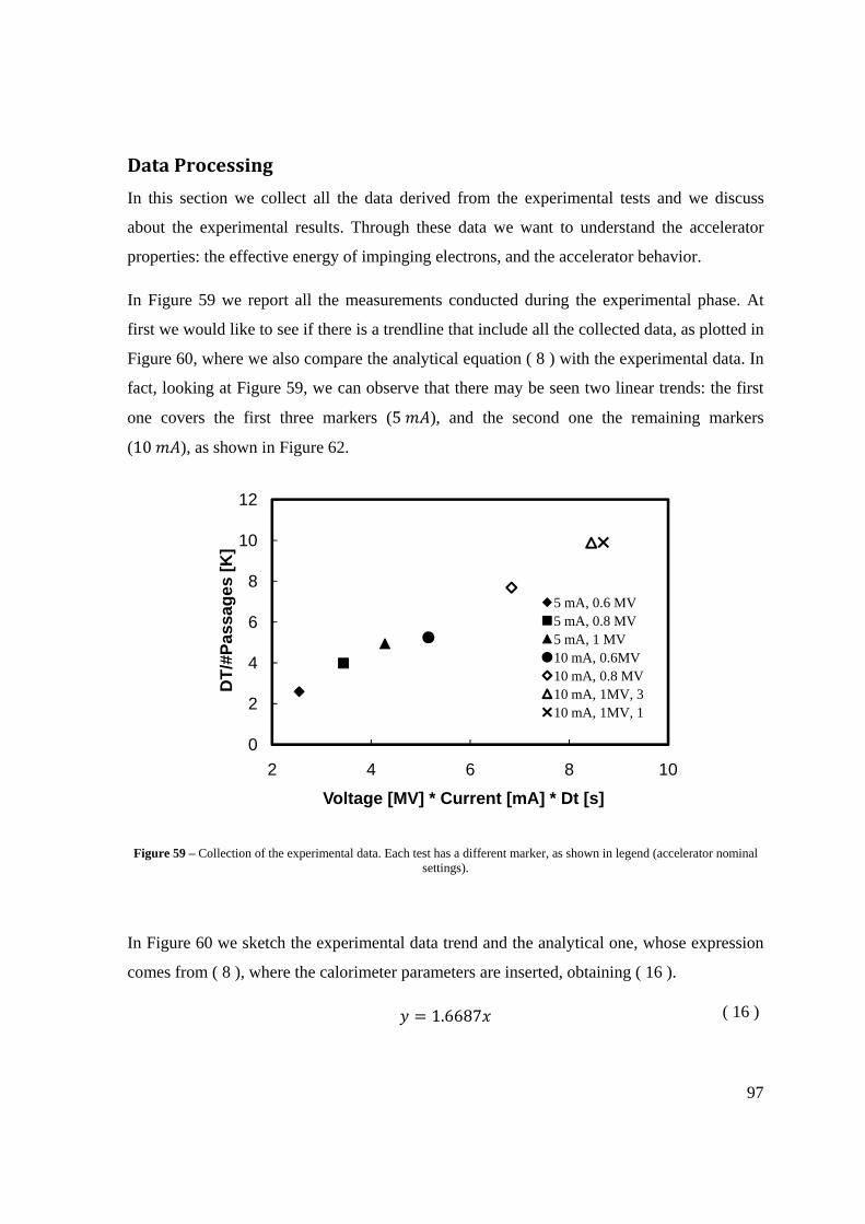
97
Data Processing
In this section we collect all the data derived from the experimental tests and we discuss
about the experimental results. Through these data we want to understand the accelerator
properties: the effective energy of impinging electrons, and the accelerator behavior.
In Figure 59 we report all the measurements conducted during the experimental phase. At
first we would like to see if there is a trendline that include all the collected data, as plotted in
Figure 60, where we also compare the analytical equation ( 8 ) with the experimental data. In
fact, looking at Figure 59, we can observe that there may be seen two linear trends: the first
one covers the first three markers (5 ), and the second one the remaining markers
(10 ), as shown in Figure 62.
Figure 59 – Collection of the experimental data. Each test has a different marker, as shown in legend (accelerator nominal settings).
In Figure 60 we sketch the experimental data trend and the analytical one, whose expression
comes from ( 8 ), where the calorimeter parameters are inserted, obtaining ( 16 ).
1.6687 ( 16 )
0
2
4
6
8
10
12
2 4 6 8 10
DT/
#Pas
sage
s [K
]
Voltage [MV] * Current [mA] * Dt [s]
5 mA, 0.6 MV5 mA, 0.8 MV5 mA, 1 MV10 mA, 0.6MV10 mA, 0.8 MV10 mA, 1MV, 310 mA, 1MV, 1
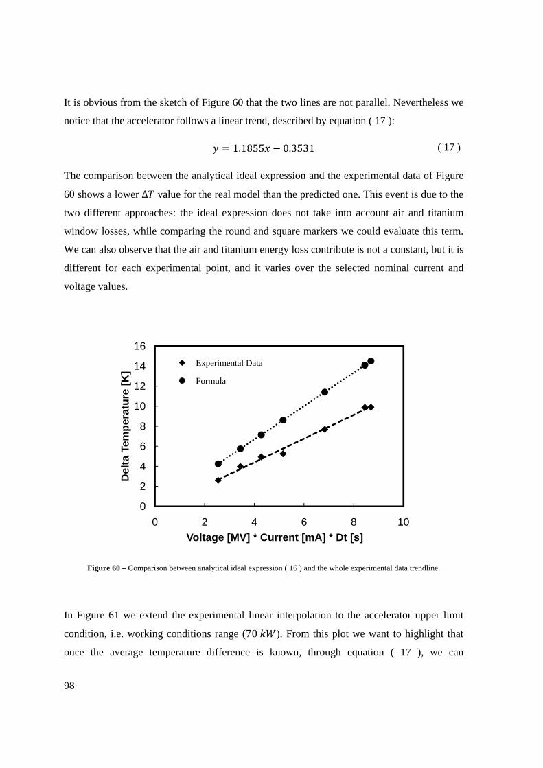
98
It is obvious from the sketch of Figure 60 that the two lines are not parallel. Nevertheless we
notice that the accelerator follows a linear trend, described by equation ( 17 ):
1.1855 0.3531
The comparison between the analytical ideal expression and the experimental data of Figure
60 shows a lower Δ value for the real model than the predicted one. This event is due to the
two different approaches: the ideal expression does not take into account air and titanium
window losses, while comparing the round and square markers we could evaluate this term.
We can also observe that the air and titanium energy loss contribute is not a constant, but it is
different for each experimental point, and it varies over the selected nominal current and
voltage values.
Figure 60 – Comparison between analytical ideal expression ( 16 ) and the whole experimental data trendline.
In Figure 61 we extend the experimental linear interpolation to the accelerator upper limit
condition, i.e. working conditions range (70 ). From this plot we want to highlight that
once the average temperature difference is known, through equation ( 17 ), we can
( 17 )
0
2
4
6
8
10
12
14
16
0 2 4 6 8 10
Del
ta T
empe
ratu
re [K
]
Voltage [MV] * Current [mA] * Dt [s]
Experimental Data
Formula
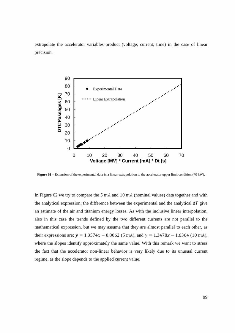
99
extrapolate the accelerator variables product (voltage, current, time) in the case of linear
precision.
Figure 61 – Extension of the experimental data in a linear extrapolation to the accelerator upper limit condition (70 kW).
In Figure 62 we try to compare the 5 and 10 (nominal values) data together and with
the analytical expression; the difference between the experimental and the analytical Δ give
an estimate of the air and titanium energy losses. As with the inclusive linear interpolation,
also in this case the trends defined by the two different currents are not parallel to the
mathematical expression, but we may assume that they are almost parallel to each other, as
their expressions are: 1.3574 0.8062 (5 ), and 1.3478 1.6364 (10 ),
where the slopes identify approximately the same value. With this remark we want to stress
the fact that the accelerator non-linear behavior is very likely due to its unusual current
regime, as the slope depends to the applied current value.
0
10
20
30
40
50
60
70
80
90
0 10 20 30 40 50 60 70
DT/
#Pas
sage
s [K
]
Voltage [MV] * Current [mA] * Dt [s]
Experimental Data
Linear Extrapolation

100
Figure 62 – Comparison between experimental data trendline and analytical ideal expression ( 16 ).
Finally in Figure 63 we plot the correlation between the imposed beam energy value and the
measured one. The derived electron beam energy holds the contribute of both the directly
calorimeter measurement and the estimated error corrections. The difference between the
imposed and the corrected values varies from 27% (1 ), to 35% (0.6 ).
The lower evaluation of the electron beam energy is one of the most important results of the
entire experiment: the imposed beam energy does not represent the same energy value at
which cables are irradiated for the crosslinking processes. As a matter of fact during the tests
the calorimeter is irradiated instead of cables and it detects the same electron energy that
cables receive while they are irradiated. With this knowledge we are able to characterize the
radiation source, so that we may possibly make more suitable corrections on the accelerator
parameters to obtain expected results for the required application needs.
0
2
4
6
8
10
12
14
16
2 4 6 8 10
Del
ta T
empe
ratu
re [K
]
Voltage [MV] * Current [mA] * Dt [s]
5 mA10 mAFormula
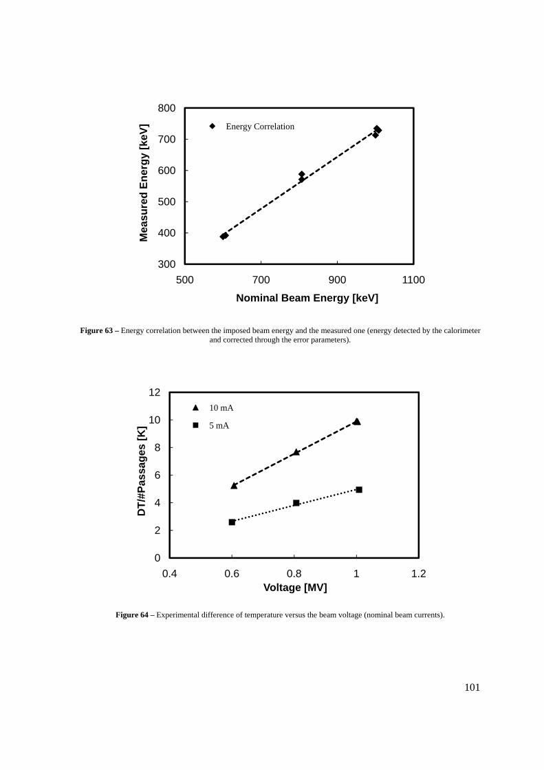
101
Figure 63 – Energy correlation between the imposed beam energy and the measured one (energy detected by the calorimeter and corrected through the error parameters).
Figure 64 – Experimental difference of temperature versus the beam voltage (nominal beam currents).
300
400
500
600
700
800
500 700 900 1100
Mea
sure
d En
ergy
[keV
]
Nominal Beam Energy [keV]
Energy Correlation
0
2
4
6
8
10
12
0.4 0.6 0.8 1 1.2
DT/
#Pas
sage
s [K
]
Voltage [MV]
10 mA
5 mA
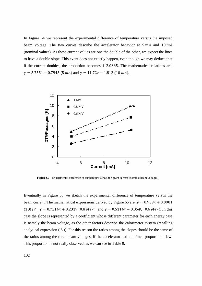
102
In Figure 64 we represent the experimental difference of temperature versus the imposed
beam voltage. The two curves describe the accelerator behavior at 5 and 10
(nominal values). As these current values are one the double of the other, we expect the lines
to have a double slope. This event does not exactly happen, even though we may deduce that
if the current doubles, the proportion becomes 1: 2.0365. The mathematical relations are:
5.7551 0.7945 (5 ) and 11.72 1.813 (10 ).
Figure 65 – Experimental difference of temperature versus the beam current (nominal beam voltages).
Eventually in Figure 65 we sketch the experimental difference of temperature versus the
beam current. The mathematical expressions derived by Figure 65 are: 0.939 0.0901
(1 ), 0.7214 0.2319 (0.8 , and 0.5114 0.0548 (0.6 ). In this
case the slope is represented by a coefficient whose different parameter for each energy case
is namely the beam voltage, as the other factors describe the calorimeter system (recalling
analytical expression ( 8 )). For this reason the ratios among the slopes should be the same of
the ratios among the three beam voltages, if the accelerator had a defined proportional law.
This proportion is not really observed, as we can see in Table 9.
0
2
4
6
8
10
12
4 6 8 10 12
DT/
#Pas
sage
s [K
]
Current [mA]
1 MV
0.8 MV
0.6 MV

103
Table 9 Slope ratios of Figure 65 compared to voltage ratios.
Beam Voltage Slope Voltage Ratio Slope Ratio Difference
/ %
1 0.939 0.8 0.7683 3.97
0.8 0.7214 0.75 0.7089 5.48
0.6 0.5114 0.6 0.5446 9.23
From Table 9 we can notice that there is not a well defined proportional law ratio that relates
the voltages to the slopes, even though from Figure 65 we see the three different slopes
associated to the three different applied beam voltages.
In the end we may assert the calorimeter linearity and the non-linear accelerator behavior
probably due to the fact that the accelerator is working in a non usual current regime.
Experiment Reproducibility
As our calorimeter is an original tool, we want to test its reproducibility: we have repeated
some experiments, and got proof that the differences between the first and the second batch
of measures are almost negligible.
In Figure 66 we plot the new carried out tests: we want to highlight that we do not need to
prove the accelerator linearity with different beam currents anymore, so that we only perform
one measurement at 5 with 1 beam voltage; the other three measures have the same
10 beam current with the three different beam voltages: 0.6 , 0.8 , and 1 .

104
Figure 66 – Collection of the second experiment data. Each test has a different marker, as shown in legend (nominal values).
Figure 67 – Focus on the 10 mA beam current data with further representation of linear interpolation.
0
2
4
6
8
10
12
2 4 6 8 10
DT/
#Pas
sage
s [K
]
Voltage [MV] * Current [mA] * Dt [s]
10 mA, 0.6 MV
10 mA, 0.8 MV
10 mA, 1 MV
5 mA, 1 MV
4
5
6
7
8
9
10
11
4 5 6 7 8 9 10
DT/
#Pas
sage
s [K
]
Voltage [MV] * Current [mA] * Dt [s]
10 mA
Linear Interpolation
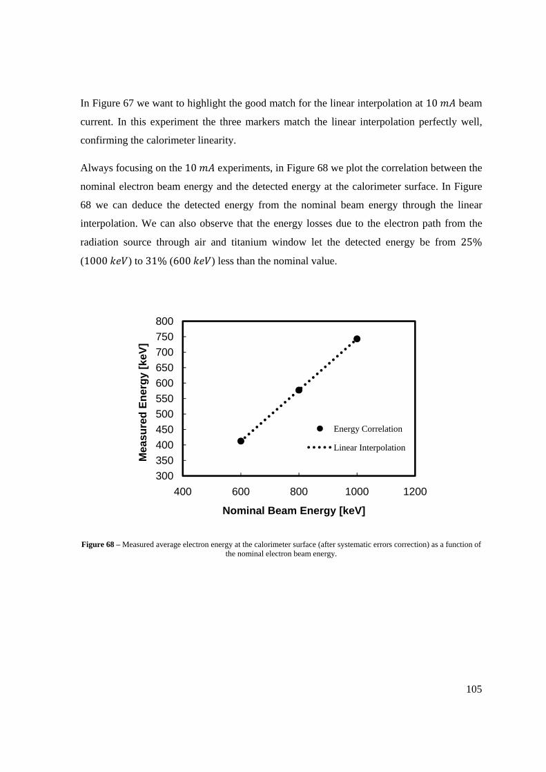
105
In Figure 67 we want to highlight the good match for the linear interpolation at 10 beam
current. In this experiment the three markers match the linear interpolation perfectly well,
confirming the calorimeter linearity.
Always focusing on the 10 experiments, in Figure 68 we plot the correlation between the
nominal electron beam energy and the detected energy at the calorimeter surface. In Figure
68 we can deduce the detected energy from the nominal beam energy through the linear
interpolation. We can also observe that the energy losses due to the electron path from the
radiation source through air and titanium window let the detected energy be from 25%
(1000 ) to 31% (600 ) less than the nominal value.
Figure 68 – Measured average electron energy at the calorimeter surface (after systematic errors correction) as a function of the nominal electron beam energy.
300350400450500550600650700750800
400 600 800 1000 1200
Mea
sure
d En
ergy
[keV
]
Nominal Beam Energy [keV]
Energy Correlation
Linear Interpolation

106
All the experimental data and the estimated energy values collected during the second batch
of experiments are summarized in Table 10.
Table 10 Calorimeter second batch Experimental Data.
Test
Nominal
Values
Total
Average Δ #
Average
Experimental
Current
Average
Experimental
Voltage
Corrected
Energy
, , #
0.6, 10, 4 22 5.5 10.34 0.6078 412 16
0.8, 10, 4 30.97 7.74 10.3 0.8075 577 16
1, 10, 3 30 10 10.27 1.02 743 17
1, 5, 3 13.97 4.66 4.92 1.017 722 32
Results & Discussion
The calorimeter experimental tests presented above show that our system has been
successfully designed for the considered energy and current electron ranges. As seen from
the previous data and graphs, the final result of the experimental phase lies in lower
accelerator electron beam energies, if compared to the nominal set-up values. The
reproducibility of the system has also been verified with two batches of experiments, proving
the extrapolation of compatible temperatures and doses.
Through the collected temperature data and equation ( 7 ), we are able to trace back the
average absorbed dose value in the aluminum calorimeter, with which we can calibrate
EBXLINK 1D simulator, obtaining the real accelerator energy. After having calibrated the
simulator accelerator energy through the calorimeter, energies reported in Table 11, we need
a model validation, since our calorimeter has been developed with a new approach. The
calorimeter measures proof has been established through data collected by the calorimeter

107
itself and another original tool, consisting of dedicated polyethylene tablets with thin film
dosimeters. The comparison between the energy data detected by the two independent
measures (integral dose calorimeter and thin film dosimeters) demonstrates an excellent
agreement, as shown in Table 11, proving the calorimeter feasibility for the considered
application dose range.
Table 11 Comparison of the Accelerator Electron Beam Energy among the nominal, the calorimeter and the dosimeters values.
Nominal EB Energy Calorimeter EB Energy Dosimeter EB Energy
1000 860 875
800 705 700
600 555 530
In Table 11 is represented the most important result of all the measurements: the real
accelerator electron beam energy has a lower value than the nominal one, whose energy
difference can be estimated within 12.5%. For the optimization of wires and cables
crosslinking this result must be seriously taken into account, if higher performances for
special industrial applications (aero-space, solar cells, railway, automotive) must be reached.
The results of this thesis have been published in the paper “Experimental Extraction of
Accelerator Parameters for Accurate Model Calibration in the Numerical 3D Simulation of
Electron Beam Crosslinking of Cables and Wires” by M. Ciappa, L. Mangiacapra, A. Lupi,
(extended abstract in Appendix – A.4) which has been accepted for presentation at the “9th
Ionizing Radiation & Polymer Symposium”, October 25-29, 2010, College Park (MD), USA.

108
Expanded Polystyrene Overheating
After several passages under the electron beam, we notice that the EPS layer in the wooden
box has been modified, as we can see in Figure 69. For this reason we investigate the causes
of the heating dissipation, as it seems that some EPS parts have reached a very high
temperature, so that they melt and become yellow. Through Monte Carlo simulations at
1 beam energy and 10 beam current, we carry out the Absorbed Dose profile in an
EPS block with 30 thickness, presented in Figure 70. As we can see from the absorbed
dose trend, the dose peak value is 52.4 , reached at 6.15 thickness.
Figure 69 – Expanded Polystyrene melting after several passages under the electron beam. The consequences of the radiation can be seen in the yellow ocher color of EPS and in the four melted zones around the aluminum calorimeter.
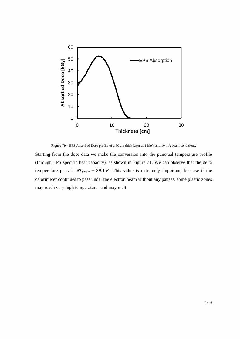
109
Figure 70 – EPS Absorbed Dose profile of a 30 cm thick layer at 1 MeV and 10 mA beam conditions.
Starting from the dose data we make the conversion into the punctual temperature profile
(through EPS specific heat capacity), as shown in Figure 71. We can observe that the delta
temperature peak is Δ 39.1 . This value is extremely important, because if the
calorimeter continues to pass under the electron beam without any pauses, some plastic zones
may reach very high temperatures and may melt.
0
10
20
30
40
50
60
0 10 20 30
Abs
orbe
d D
ose
[kG
y]
Thickness [cm]
EPS Absorption

110
Figure 71 – EPS Temperature profile of a 30 cm thick layer.
As our model does not only consist of EPS (calorimeter sides), we run another simulation
more similar to our sample: it consists of 3 EPS layer and 1 graphite layer (in the real
model there is the wooden bottom box). These results are plotted in Figure 72. We choose the
graphite, because it has a behavior close to wood, above all for the backscattering properties.
From Figure 72 we can see that the dose peak is reached in graphite and that the EPS
behavior is very similar to the case only consisting of EPS (Figure 70). In the EPS and
graphite model, the dose peak in expanded polystyrene is 41.56 , to which
corresponds a delta temperature peak Δ 31 . This evaluation makes us aware that if
the calorimeter box passes for instance 10 times under the accelerator, the delta temperature
peak reaches Δ 310 , that means complete polystyrene melting in the interested
zones.
Therefore we decide to impose a limit of almost consecutive passages under the radiation
source of six times, so that the maximum temperature increase is around 200 .
0
5
10
15
20
25
30
35
40
45
0 10 20 30
Del
ta T
empe
ratu
re [K
]
Thickness [cm]
EPS Temperature

111
Figure 72 – Absorbed Dose profile in a 3 cm EPS layer followed by a 1 cm graphite layer at 1 MeV and 10 mA beam conditions.
05
101520253035404550
0 1 2 3 4
Abs
orbe
d D
ose
[kG
y]
Thickness [cm]
EPS and Graphite

112
113
Conclusions
The entire work focuses on the modeling and development of an aluminum integral dose
calorimeter for polymers crosslinking, whose design and test deal with dosimetry
measurements at 0.5 2 electron beam energy range.
Our investigations and analyses prove that our calorimeter has been successfully designed
meeting the specifications for the examined industrial environment. The most important
result consists of the quite high difference between the imposed beam energy and the
detected one, meaning that the radiation energy detected by the cable during the crosslinking
process is lower than the expected one, causing loss in performances, if this correction is not
adequately taken into account.
To give evidence of our analyses, we compare the calorimeter measurements with another
original tool composed of dedicated polyethylene tablets with thin film dosimeters. The
comparison between the energy data detected by the two independent measures demonstrates
an excellent agreement, proving the calorimeter feasibility for the considered application
dose range and lower electron beam energy than the nominal one.
With the knowledge of the real electron beam energy value and the accelerator behavior we
are able to characterize the radiation source, so that we can make more suitable corrections
on the imposed accelerator parameters to obtain appropriate results for the required
application field.
The prospective improvement of our calorimeter lies in solving some material and
mechanical challenges to make the system more suitable to the accelerator physical
characteristics: a more compact geometry, the use of screws instead of glue and the radiation
resistance improvement of the insulation layer because of the high reached temperatures
114
(several passages under the radiation source), and a proper system for damping conveyor
oscillations.
Another possible step for the calorimetric measurements enhancement consists of finalizing
the water calorimeter as an absolute reference, since it has already been designed and it only
requires assembly and testing.
The future development of our integral dose calorimeter may be based on analyses and tests
of new radiation sources at higher beam current levels, whose properties are requested for
more accurate industrial processes, such as cables and wires crosslinking.
Our integral dose calorimeter has the potential of being developed into a standard for electron
accelerator characterization, performance, and maintenance in industrial environment.
The results of this thesis have finally been published in the paper “Experimental Extraction
of Accelerator Parameters for Accurate Model Calibration in the Numerical 3D Simulation of
Electron Beam Crosslinking of Cables and Wires” by M. Ciappa, L. Mangiacapra, A. Lupi,
(extended abstract in Appendix – A.4) which has been accepted for presentation at the “9th
Ionizing Radiation & Polymer Symposium”, October 25-29, 2010, College Park (MD), USA.

115
Appendix – A.1
CSDA Graphs
When dimensioning the calorimeter, we use as an important parameter the CSDA
(Continuous Slow Down Approximation) electron range, which is a calculated quantity that
represents the mean path length along the electrons trajectory. In the following graphs we
plot the CSDA range for the different materials that we needed for our analysis from 0
to 10 , i.e. graphite in Figure 73, aluminum in Figure 74, copper in Figure 75,
polyethylene (PE) in Figure 76, polystyrene (PS) in Figure 77, and mylar in Figure 78. All
the data are collected through ESTAR software developed by NIST (National Institute of
Standards and Technology – Physics Laboratories).
Figure 73 – Graphite CSDA electron range.
0
0.01
0.02
0.03
0.04
0.05
0.06
0.07
0 2 4 6 8 10 12
Ran
ge [c
m]
Energy [MeV]
Graphite CSDA

116
Figure 74 – Aluminum CSDA electron range.
Figure 75 – Copper CSDA electron range.
0
0.005
0.01
0.015
0.02
0.025
0.03
0 2 4 6 8 10 12
Ran
ge [c
m]
Energy [MeV]
Aluminum CSDA
0
0.2
0.4
0.6
0.8
1
1.2
1.4
1.6
0 2 4 6 8 10 12
Ran
ge [c
m]
Energy [MeV]
Copper CSDA
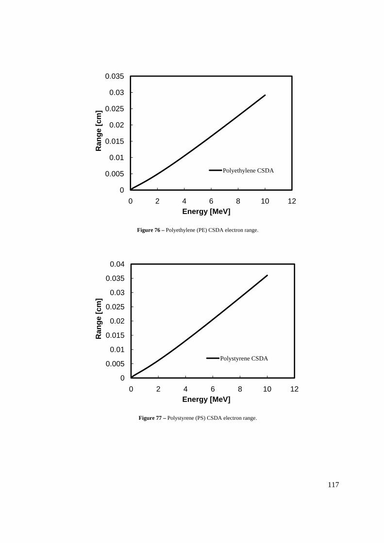
117
Figure 76 – Polyethylene (PE) CSDA electron range.
Figure 77 – Polystyrene (PS) CSDA electron range.
0
0.005
0.01
0.015
0.02
0.025
0.03
0.035
0 2 4 6 8 10 12
Ran
ge [c
m]
Energy [MeV]
Polyethylene CSDA
0
0.005
0.01
0.015
0.02
0.025
0.03
0.035
0.04
0 2 4 6 8 10 12
Ran
ge [c
m]
Energy [MeV]
Polystyrene CSDA

118
Figure 78 – Mylar CSDA electron range.
0
0.005
0.01
0.015
0.02
0.025
0.03
0.035
0.04
0.045
0 2 4 6 8 10 12
Ran
ge [g
/cm
2 ]
Energy [MeV]
Mylar CSDA
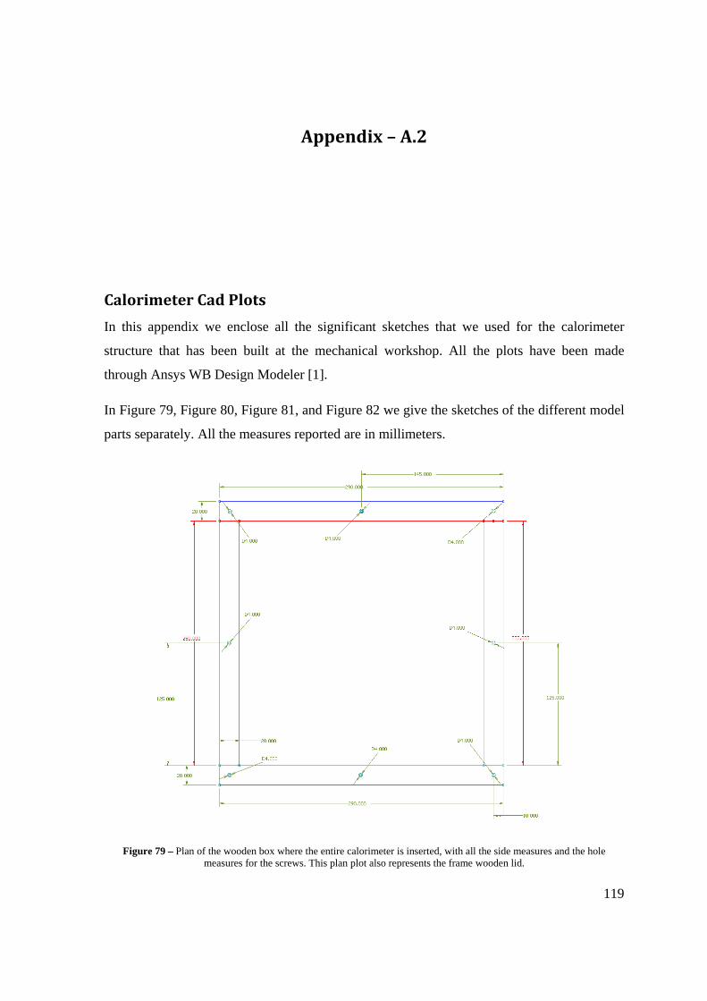
119
Appendix – A.2
Calorimeter Cad Plots
In this appendix we enclose all the significant sketches that we used for the calorimeter
structure that has been built at the mechanical workshop. All the plots have been made
through Ansys WB Design Modeler [1].
In Figure 79, Figure 80, Figure 81, and Figure 82 we give the sketches of the different model
parts separately. All the measures reported are in millimeters.
Figure 79 – Plan of the wooden box where the entire calorimeter is inserted, with all the side measures and the hole measures for the screws. This plan plot also represents the frame wooden lid.
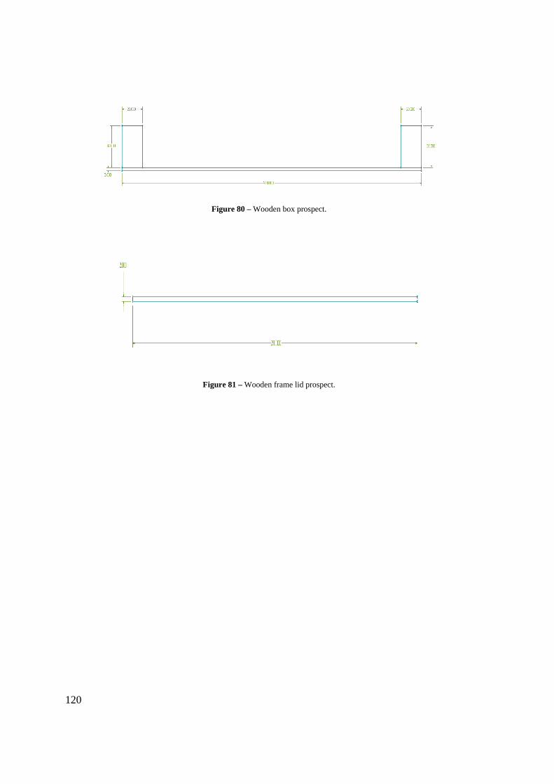
120
Figure 80 – Wooden box prospect.
Figure 81 – Wooden frame lid prospect.

121
Figure 82 – Aluminum Calorimeter representation with the 3 cm length hole for the capillary where it is inserted the Micro-BetaCHIP thermistor.
In Figure 83 we report the plot of the entire calorimetric system without mylar foil cover.
Figure 83 – Three dimensional view of the entire calorimetric system: wooden box, EPS insulation (inside the box), and the aluminum absorber, represented by the cylinder in the middle of the model.

122
123
Appendix – A.3
Matlab file
As previously written in Chapter 4, our Matlab file is a mean to establish the energy of
impinging electrons taking into account energy errors and losses due to the designed system
(mylar absorption, electron backscattering, boundary escapes, Bremsstrahlung emission,
Micro-BetaCHIP tolerance, interpolation error).
In the Matlab file we also decide to evaluate the average dose deposed by the electron beam.
As the dose is entirely deposited within the CSDA range, we need to rearrange equations
presented in Chapter 1, as follows in equation ( 18 ):
Δ Δ ·
where Δ is the difference of temperature within the CSDA range , Δ is the total
difference of temperature , is the total calorimeter thickness , and is the
calorimeter CSDA thickness .
And the average dose is given in ( 19 ).
· · · Δ
· · · Δ
where is the average dose value within the CSDA , is the total absorbed
energy , is the mass defined by CSDA range , is the material specific heat
capacity ·
, and the material density .
In Table 12 we collect all the dose data derived by ( 19 ) for the different experiments.
( 18 )
( 19 )

124
Table 12 Average Absorbed Dose values of the experimental tests.
Test Average Dose
, , #
1, 10, 3 29.06
0.8, 10, 3 31.46
0.6, 10, 3 36.26
1, 5, 6 14.68
0.8, 5, 3 15.68
0.6, 5, 6 18.17
1, 10, 1 30.26
In the following lines we attach the Matlab script.
clc clear all; % Program to compute the Absorbed Energy value within the Aluminum Calorimeter %************************************************************************* % INPUT Measured Temperature Difference %************************************************************************* delta_T = 9.9; % Temperature Difference [K] %************************************************************************* %************************************************************************* % INPUT Electron Beam Parameters %************************************************************************* E_acc = 1; % Energy Accelerator [MeV] t_tran = 0.82; % transit time [s] beam_curr_mA = 10.6; % beam current [mA] A_irr = 540; % Irradiated Area [cm2] %*************************************************************************

125
%************************************************************************* % INPUT Calorimetric System Parameters % ************************************************************************ roAL = 2.71; % density [g/cm3] CpAL = 0.9; % spec. heat Aluminum [J/(g K)] t_cal = 0.45; % cal thickness [cm] % ************************************************************************ % ************************************************************************ % OUTPUT: Measured Energy without corrections (Ideal) % ************************************************************************ display('**************************************************************'); display('Non Correctrd Acceleration Energy from Calorimeter [keV]'); display('**************************************************************'); E_cal_ideal = delta_T* roAL * t_cal * CpAL *A_irr/ ( beam_curr_mA * t_tran ) % [keV] % ************************************************************************ % ************************************************************************ % Mylar films Correction % ************************************************************************ display('**************************************************************'); display('Correction for Mylar Absorption [keV]'); display('**************************************************************'); E_Loss_M_6um = 0.0502*E_acc^6 - 0.5607*E_acc^5 + 2.5471 * E_acc^4 - 6.0688*E_acc^3 + 8.1083*E_acc^2 - 5.851*E_acc + 4.357 % Energy Loss in mylar [keV] % ************************************************************************ % ************************************************************************ % Backscattering Correction % ************************************************************************ display('**************************************************************'); display('Correction for Energy Loss due to Electron Backscattering [keV]'); display('**************************************************************'); E_backsc_per = 0.0407*E_acc^4 - 0.4136*E_acc^3 + 1.9788*E_acc^2 - 5.4835*E_acc + 7.9465; % %Backscattering energy loss [%] E_backsc_p = E_backsc_per/100; % %Backscattering energy loss [%]
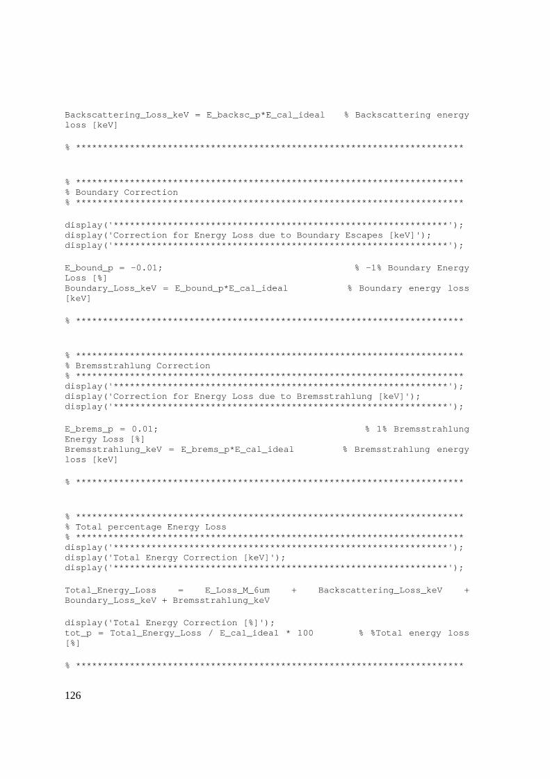
126
Backscattering_Loss_keV = E_backsc_p*E_cal_ideal % Backscattering energy loss [keV] % ************************************************************************ % ************************************************************************ % Boundary Correction % ************************************************************************ display('**************************************************************'); display('Correction for Energy Loss due to Boundary Escapes [keV]'); display('**************************************************************'); E_bound_p = -0.01; % -1% Boundary Energy Loss [%] Boundary_Loss_keV = E_bound_p*E_cal_ideal % Boundary energy loss [keV] % ************************************************************************ % ************************************************************************ % Bremsstrahlung Correction % ************************************************************************ display('**************************************************************'); display('Correction for Energy Loss due to Bremsstrahlung [keV]'); display('**************************************************************'); E_brems_p = 0.01; % 1% Bremsstrahlung Energy Loss [%] Bremsstrahlung_keV = E_brems_p*E_cal_ideal % Bremsstrahlung energy loss [keV] % ************************************************************************ % ************************************************************************ % Total percentage Energy Loss % ************************************************************************ display('**************************************************************'); display('Total Energy Correction [keV]'); display('**************************************************************'); Total_Energy_Loss = E_Loss_M_6um + Backscattering_Loss_keV + Boundary_Loss_keV + Bremsstrahlung_keV display('Total Energy Correction [%]'); tot_p = Total_Energy_Loss / E_cal_ideal * 100 % %Total energy loss [%] % ************************************************************************
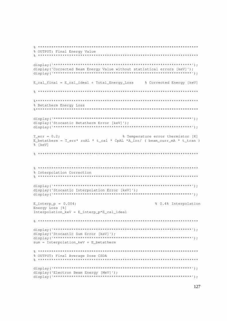
127
% ************************************************************************ % OUTPUT: Final Energy Value % ************************************************************************ display('**************************************************************'); display('Corrected Beam Energy Value without statistical errors [keV]'); display('**************************************************************'); E_cal_final = E_cal_ideal + Total_Energy_Loss % Corrected Energy [keV] % ************************************************************************ %************************************************************************* % Betatherm Energy Loss %************************************************************************* display('**************************************************************'); display('Stocastic Betatherm Error [keV]'); display('**************************************************************'); T_err = 0.2; % Temperature error thermistor [K] E_betatherm = T_err* roAL * t_cal * CpAL *A_irr/ ( beam_curr_mA * t_tran ) % [keV] % ************************************************************************ % ************************************************************************ % Interpolation Correction % ************************************************************************ display('**************************************************************'); display('Stocastic Interpolation Error [keV]'); display('**************************************************************'); E_interp_p = 0.004; % 0.4% Interpolation Energy Loss [%] Interpolation_keV = E_interp_p*E_cal_ideal % ************************************************************************ display('**************************************************************'); display('Stocastic Sum Error [keV]'); display('**************************************************************'); sum = Interpolation_keV + E_betatherm % ************************************************************************ % OUTPUT: Final Average Dose CSDA % ************************************************************************ display('**************************************************************'); display('Electron Beam Energy [MeV]'); display('**************************************************************');
128
Eb = E_cal_final/1000 % Energy beam [MeV] CSDA_Energy_trasp = [3.000E-01 1.083E-01, 3.500E-01 1.361E-01, 4.000E-01 1.652E-01, 4.500E-01 1.952E-01, 5.000E-01 2.260E-01, 5.500E-01 2.575E-01, 6.000E-01 2.894E-01, 7.000E-01 3.545E-01, 8.000E-01 4.206E-01, 9.000E-01 4.874E-01, 1.000E+00 5.546E-01, 1.250E+00 7.231E-01, 1.500E+00 8.913E-01, 1.750E+00 1.058E+00, 2.000E+00 1.224E+00, 2.500E+00 1.550E+00, 3.000E+00 1.869E+00, 3.500E+00 2.183E+00, 4.000E+00 2.491E+00, 4.500E+00 2.794E+00, 5.000E+00 3.092E+00]; CSDA_Energy = CSDA_Energy_trasp'; CSDA_Energy(2,:) = CSDA_Energy(2,:) ./ roAL; display('**************************************************************'); display('CSDA Evaluated Thickness [cm]'); display('**************************************************************'); CSDA_Eb = interp1(CSDA_Energy(1,:),CSDA_Energy(2,:),Eb) display('**************************************************************'); display('Average CSDA Dose CSDA Value [kGy]'); display('**************************************************************'); D_CSDA = CpAL * delta_T * t_cal / CSDA_Eb % Average Dose [kGy] % ************************************************************************

129
Appendix – A.4
Extended Abstract
The results of this thesis have been published in the paper “Experimental Extraction of
Accelerator Parameters for Accurate Model Calibration in the Numerical 3D Simulation of
Electron Beam Crosslinking of Cables and Wires” by M. Ciappa, L. Mangiacapra, A. Lupi,
which has been accepted for presentation at the “9th Ionizing Radiation & Polymer
Symposium”, October 25-29, 2010, College Park (MD), USA.
In this section we attach the extended abstract of the paper.

130
131
Bibliography
[1] F. Dadkhah, J. Zecher. ANSYS Workbench Software Release 12, Tutorial with Multimedia CD. SDC Publications, 2009.
[2] Radiation Dosimetry: Electron Beams with Energies Between 1 and 50 MeV. ICRU Report 35, International Commission on Radiation Units and Measurements, 1984, 14-15, 77-80, 92-95.
[3] ISO/ASTM 51631 Practice for use of calorimetric dosimetry system for electron beam dose measurements and dosimeter calibrations. International Standard ISO/ASTM 51631, ISO/ASTM International 2003, 2003.
[4] Dosimetry Systems. Report 80, Journal of the ICRU, Vol 8, No 2, 2008, 33-37.
[5] J. S. Laughlin, S. Genna. "Calorimetry." In Radiation Dosimetry Instrumentation, Vol 2, by W. C. Roesch F. H. Attix, 389-439. 1966-1972.
[6] A. Miller, A. Kovacs. "Calorimetry at industrial electron accelerators." Nuclear Instrumentation and Methods in Physics Reseach B10/11 (1985): 994-997.
[7] I. Janovsky, A. Miller. "A Calorimeter for Measuring Energy Deposition in Materials and Calibrating the Response of Dosimeters Irradiated by Low-Energy Industrial Electron Accelerators." Applied Radiation and Isotopes 38, no. 11 (1987): 931-937.
[8] A. Miller, A. Kovacs, F. Kuntz. "Development of a polystyrene calorimeter for application at electron energies down to 1.5 MeV." Radiation Physics and Chemistry, 2002: 739-744.
132
[9] Miller, A. "Polystyrene Calorimeter for Electron Beam Dose Measurements." Radiation Physics and Chemistry 46, no. 4-6 (1995): 1243-1246.
[10] A. Miller, A. Kovacs. "Application of Calorimeters for Routine and Reference Dosimetry at 4-10 MeV Industrial Electron Accelerators." Radiation Physics and Chemistry 35, no. 4-6 (1990): 774-778.
[11] J. C. Humphreys, W. L. McLaughlin. "Calorimetry of Electron Beams and the Calibration of Dosimeters at High Doses." Radiation Physics and Chemistry 35, no. 4-6 (1990): 744-749.
[12] J. Helt-Hansen, A. Miller, S. Duane, P. Sharpe, M. McEwen, S. Cluasen. "Calorimetry for dose measurement at electron accelerators in the 80-120 keV range." Radiation Physics and Chemistry 74 (2005): 354-371.
[13] Micro-BetaCHIP Thermistor Probe. "http://www.meas-spec.com/product."
[14] NI ENET-9219. "http://sine.ni.com/nips/cds/view/p/lang/en/nid/205700." http://www.ni.com/.