Ninth International Geostatistics Congress, Oslo, Norway June 11 – 15, 2012

Modeling Dependencies Between oil Exploration

Prospects with Bayesian Networks

Ragnar Hauge1, Marita Stien2, Maren Drange-Espeland3, Jo Eidsvik4 and Gabriele

Martinelli5

Abstract Oil exploration prospects in an area are typically dependent due to

common geological factors. These dependencies can have major impact on how a

drilling program should be carried out in the area in order to maximize the

income. Despite this, oil companies tend to use these dependencies only to update

marginal discovery probabilities after a well has been drilled. The main reason for

this is that this is done ad hoc based on the geological understanding, without an

explicit underlying model. Thus, exploring possibilities in advance of drilling

becomes too time consuming. We show how Bayesian networks can be used to

capture and summarize the underlying geological dependencies in a consistent

manner. This gives a full joint probability distribution for all prospects in the area,

which easily updates when new wells are drilled. The quick and easy updating

allows testing of different exploration strategies. All elements in the network have

direct physical interpretation, making it simple both to build the networks and to

see which geological effects that have been included. The methodology has been

tested on several real world cases, and we present a case based on one of these.

Introduction

The dependencies between different prospects can have a significant impact in oil

exploration, but there is a lack of good models for these dependencies. This means

that in practice, ad hoc techniques are applied. These may be reasonable as a

response to updating probabilities when new data has arrived, but any attempt to

take the correlations into account when planning a drilling sequence will need a

fast, automatic model update. Having such a model also ensures consistency.

1 Norwegian Computing Center, PO Box 114, Blindern, N-0314 Oslo, Norway,

Ragnar.Hauge@nr.no 2 Norwegian Computing Center, PO Box 114, Blindern, N-0314 Oslo, Norway,

Marita.Stien@nr.no 3 Gassco AS, PO Box 93, N-5501 Haugesund, Norway, mdes@gassco.no 4 Department of Mathematical Sciences, NTNU, N-7491 Trondheim, joeid@math.ntnu.no 5 Department of Mathematical Sciences, NTNU, N-7491 Trondheim,

gabriele.martinelli@math.ntnu.no

2

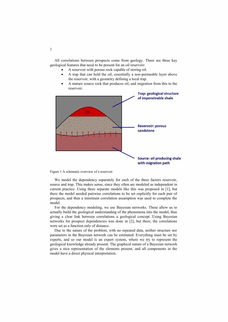
All correlations between prospects come from geology. There are three key

geological features that need to be present for an oil reservoir:

A reservoir with porous rock capable of storing oil.

A trap that can hold the oil, essentially a non-permeable layer above

the reservoir, with a geometry defining a local trap.

A mature source rock that produces oil, and migration from this to the

reservoir.

Figure 1 A schematic overview of a reservoir

We model the dependency separately for each of the three factors reservoir,

source and trap. This makes sense, since they often are modeled as independent in

current practice. Using three separate models like this was proposed in [1], but

there the model needed pairwise correlations to be set explicitly for each pair of

prospects, and then a minimum correlation assumption was used to complete the

model.

For the dependency modeling, we use Bayesian networks. These allow us to

actually build the geological understanding of the phenomena into the model, thus

giving a clear link between correlations a geological concept. Using Bayesian

networks for prospect dependencies was done in [2], but there, the correlations

were set as a function only of distance.

Due to the nature of the problem, with no repeated data, neither structure nor

parameters in the Bayesian network can be estimated. Everything must be set by

experts, and so our model is an expert system, where we try to represent the

geological knowledge already present. The graphical nature of a Bayesian network

gives a nice representation of the elements present, and all components in the

model have a direct physical interpretation.

3

We take the prior probabilities for success for each factor at each prospect as

given input, and build the correlation model without perturbing the initial values

of these. Setting these priors is a very different modeling problem, and not

discussed here.

The model presented here is also described in [3] and [4], where our example is

taken from. More details can be found in these papers. In the next section, we will

look at the qualitative concepts for building a model, and then the quantitative

aspect is discussed in the third section. Our example is presented in full in section

4, before some concluding remarks are given.

Qualitative Modeling

First, we give a brief introduction of Bayesian networks. A Bayesian network is a

directed acyclic graph, parameterized with conditional probabilities. In practice,

this means that we use a model with a set of events, and dependencies between

these. The dependencies have a direction, and there should be no circular

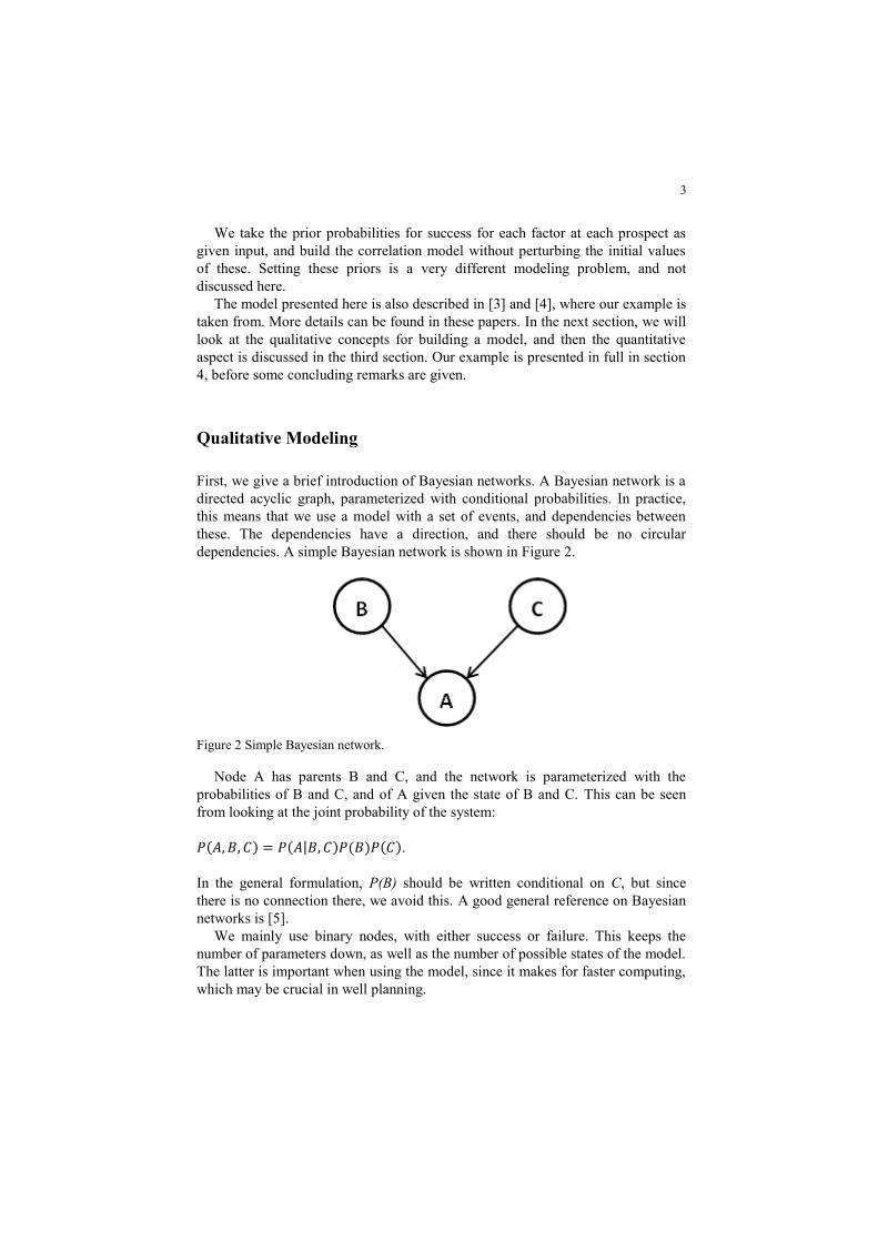
dependencies. A simple Bayesian network is shown in Figure 2.

Figure 2 Simple Bayesian network.

Node A has parents B and C, and the network is parameterized with the

probabilities of B and C, and of A given the state of B and C. This can be seen

from looking at the joint probability of the system:

( ) ( | ) ( ) ( ).

In the general formulation, P(B) should be written conditional on C, but since

there is no connection there, we avoid this. A good general reference on Bayesian

networks is [5].

We mainly use binary nodes, with either success or failure. This keeps the

number of parameters down, as well as the number of possible states of the model.

The latter is important when using the model, since it makes for faster computing,

which may be crucial in well planning.

4

There are three key concepts we use when building a network:

1. Strict and relaxed parents.

2. Local failure probabilities.

3. Common cause versus common mechanism.

In the following, we will discuss each of these.

Strict and Relaxed Parents

To simplify our model building, we use the concept of success propagation. This

means that a node cannot be a success if all its parents are failures. This modeling

approach allows us at each stage to ask which factors must be present for this node

to be a success, and thus work our way upwards in the network. This means that if

there are factors that lead to failure, we model the absence of these.

When looking at success factors, there are two types. One is where all parents

must be a success for the child to be a success, and this is what we call strict

parents. However, in some cases we may need only that one parent is a success in

order for the child to be a success, which is what we call relaxed parents. The

latter occurs in source networks, where there may be different migration paths into

an area and only one of them need to be successful.

For the relaxed parents, we assume that success propagation is independent.

This allows us to only specify the probability of success given that this parent is a

success. For strict parents, we need only one parameter for all of them, the

probability of success given that all strict parents are success. Thus, these

assumptions reduce the number of parameters to specify for a node with n parents

from 2n to at most n if all parents are relaxed.

A node may have any combination of strict and relaxed parents, and even

different groups of relaxed parent, although we have not used the latter in any of

our model so far. Note that a strict parent always is at least as probable as any of

its children, and that single parents always are strict.

Local Failure Probabilities

In practice we introduce a probability for a purely local failure, one that does not

impact the rest of the network. This makes sense geologically, since there also are

local factors having an impact on the success of a prospect. Consider a case of

modeling the reservoir factor for four prospects, where we know that the reservoir

quality is better when moving eastwards. We would then use a network like in

Figure 3.

5

Figure 3 A simple reservoir network, with a correlation layer and a prospect layer.

Note the two layers. At the bottom layer is the actual prospects, whereas the

correlations are in the top layer. There are several reasons for this, the most

compelling being that if we correlated the prospects directly, we could never have

success to the west of a failure. That does not make sense, since the failure could

be local, and not imply that there are no successful reservoirs further west.

To overcome this, we introduce the local failure probability. The top layer thus

represents the general quality in an area, so a failure there will stop all prospects

further west. At the bottom level, we have the actual prospects, and the probability

of failure at the bottom level given success at the top is the local failure

probability.

Common Cause versus Common Mechanism

So far, everything we have looked at falls into what we call common cause.

Correlations occur because two nodes share a parent, and when this parent is a

binary success or failure node, it is a common cause for what follows. In many

situations, this makes sense, like for the reservoir example above. However, in

many settings, there is no direct common factor that is either success or failure for

all descendants; instead, we have the same mechanism at work.

Consider for instance an area where the cap rock tends to be fractured. This is a

local event, so there is no direct large scale correlation. However, we have only a

vague initial guess of the probability of this, and as we observe the presence or

absence of fracturing at different prospects, we want to update this probability for

the remaining prospects. This is what we call common mechanism.

6

To represent this, we introduce the concept of a counting node. A counting

node C has K different states, and the success probability of its children Ai is the

same for all children. The children are binary nodes, and when one of them is a

success, the probability of success in the children increases and vice versa. This is

handled by setting the success probability for the children as this:

( | )

A positive observation will thus increase the probability of large k, and

decrease the probability of small values, whereas a negative observation does the

opposite. All this fits within the framework of Bayesian networks, since we here

have given the rule for the probability of the children given the parents, depending

only on the state of the parent.

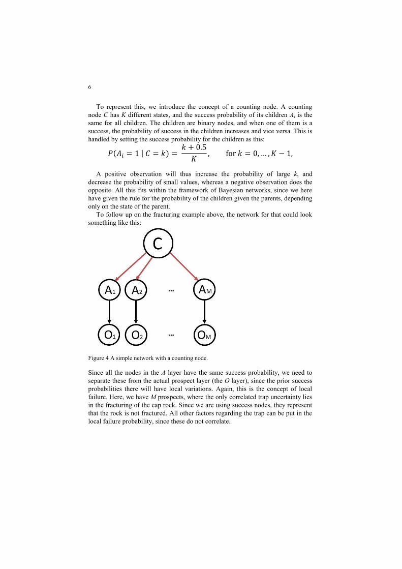
To follow up on the fracturing example above, the network for that could look

something like this:

Figure 4 A simple network with a counting node.

Since all the nodes in the A layer have the same success probability, we need to

separate these from the actual prospect layer (the O layer), since the prior success

probabilities there will have local variations. Again, this is the concept of local

failure. Here, we have M prospects, where the only correlated trap uncertainty lies

in the fracturing of the cap rock. Since we are using success nodes, they represent

that the rock is not fractured. All other factors regarding the trap can be put in the

local failure probability, since these do not correlate.

7

Quantitative Modeling

Although there can be quite a few parameters that must be set for the model, the

structure of the network makes this specification feasible. All parameters are just

local in scope, and have a direct physical interpretation – what is the probability of

a success here, given these factors.

However, there are a few global restrictions that must be kept in mind when

setting these parameters:

We must preserve the prior success probabilities at each prospect.

A strict parent must always have higher probability than its children.

No probability can be negative or larger than 1.

The latter demand may seem obvious, but due to the way these parameters are

specified, it is easy to violate. The probabilities in the bottom nodes of the network

are given, since these are the prior probabilities for the prospect. If the conditional

probabilities are set without thinking about these base probabilities, this can

quickly lead to marginal probabilities larger than 1.To avoid this, it is simplest to

start from the bottom and work upwards, ensuring at each stage that the marginal

probability for a node can be smaller than 1.

Ideally, the experts would go through each link in the system, and assign a

probability to it. However, for large networks this can be impractical. As a help

for automatically assigning probabilities in parts of the networks, we note that

there are two extreme settings available for any network: Maximizing or

minimizing the local failure probability.

If we minimize it, we get a highly correlated network. All observations get their

maximum global impact, since there is no potential of a local failure, so all

failures occur higher in the network. On the other hand, by maximizing the

probability of local failure, the network falls apart, everything is seen as a local

effect, and the higher nodes have high a priori success probabilities, with all

failures seen as local. Now observations have minimal impact.

These limits can be found, and by considering these extremes on a scale from 0

to 1, where 0 is minimal and 1 is maximal correlation, we can set up an automatic

probability distribution scheme for values in between. In addition to the

correlation value, we also need an assumption that failures are evenly distributed

among the different links in the network. This can easily be combined by explicit

specification of parts of the network.

Example

Here, we look at a local case with four prospects, and see how they correlate at

reservoir, source and trap level. We then do some simple response tests on the

network. The prior probabilities for the four prospects are given in Table 1.

8

Table 1 Prior success probabilities for the different factor at each prospect.

A B C D

Reservoir 0.60 0.80 0.40 0.80

Source 0.50 0.60 0.60 0.40

Trap 0.32 0.42 0.40 0.35

Overall 0.096 0.202 0.096 0.112

Reservoir Network

All prospects are in the same geological formation, which is getting poorer as we

move westwards. We thus get the network we used previously as an example in

Figure 3. Note that even though the general quality is expected to decrease

westwards, this does not mean that the prior probabilities must follow this trend,

and indeed, the lowest prior probability is found in the second prospect from the

east, prospect C. This low value is due to local geological considerations.

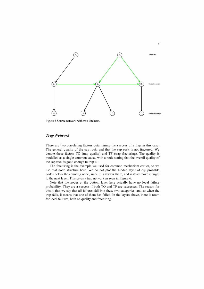
Source Network

The source network is shown in Figure 5. We have two oil producing shales

(kitchens K1 and K2), and these feed into the area of prospect A, or prospects B, C,

and D. Prospects B and C are in the same general area regarding migration, so

these have a common node in the migration layer. Oil may migrate into this area

from the area around A, and from this area to the area around D. Thus, oil from

the second kitchen can either migrate directly to the area around D, or through the

area around B and C.

Note again how all correlations are in the top two layers, while the prospect

layer with the observable nodes are at the bottom. Again, this allows for flexibility

with local failures.

The nodes in the migration layer have relaxed parents, since we only need

migration of oil from one direction in order to have success here. However, for the

area around A, there is only one migration path, and so we need success in kitchen

1 to get oil here.

9

Figure 5 Source network with two kitchens.

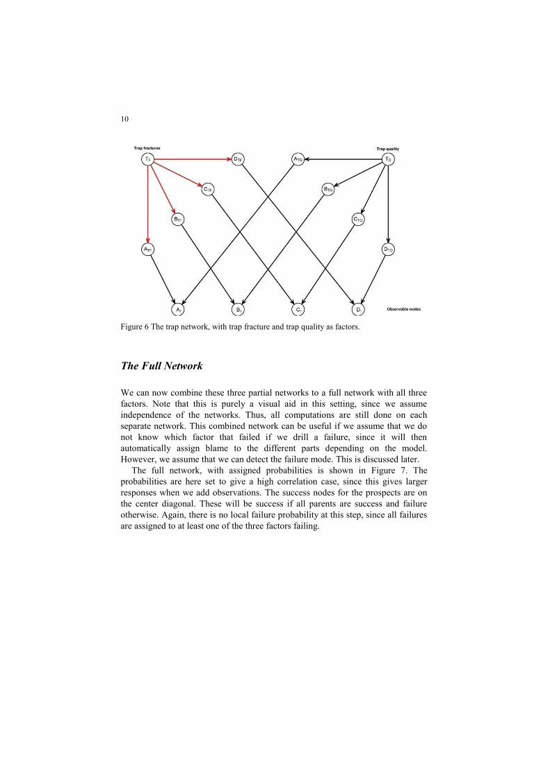
Trap Network

There are two correlating factors determining the success of a trap in this case:

The general quality of the cap rock, and that the cap rock is not fractured. We

denote these factors TQ (trap quality) and TF (trap fracturing). The quality is

modelled as a single common cause, with a node stating that the overall quality of

the cap rock is good enough to trap oil.

The fracturing is the example we used for common mechanism earlier, so we

use that node structure here. We do not plot the hidden layer of equiprobable

nodes below the counting node, since it is always there, and instead move straight

to the next layer. This gives a trap network as seen in Figure 6.

Note that the nodes at the bottom layer here actually have no local failure

probability. They are a success if both TQ and TF are successes. The reason for

this is that we say that all failures fall into these two categories, and so when the

trap fails, it means that one of them has failed. In the layers above, there is room

for local failures, both on quality and fracturing.

10

Figure 6 The trap network, with trap fracture and trap quality as factors.

The Full Network

We can now combine these three partial networks to a full network with all three

factors. Note that this is purely a visual aid in this setting, since we assume

independence of the networks. Thus, all computations are still done on each

separate network. This combined network can be useful if we assume that we do

not know which factor that failed if we drill a failure, since it will then

automatically assign blame to the different parts depending on the model.

However, we assume that we can detect the failure mode. This is discussed later.

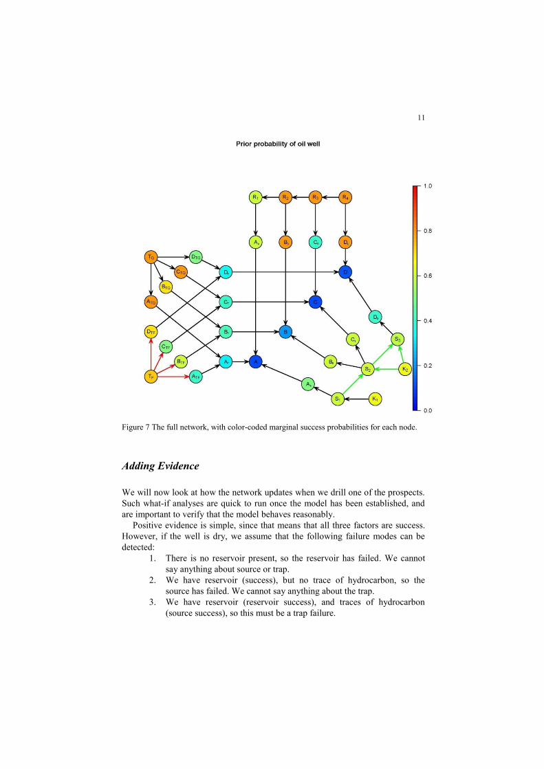
The full network, with assigned probabilities is shown in Figure 7. The

probabilities are here set to give a high correlation case, since this gives larger

responses when we add observations. The success nodes for the prospects are on

the center diagonal. These will be success if all parents are success and failure

otherwise. Again, there is no local failure probability at this step, since all failures

are assigned to at least one of the three factors failing.

11

Figure 7 The full network, with color-coded marginal success probabilities for each node.

Adding Evidence

We will now look at how the network updates when we drill one of the prospects.

Such what-if analyses are quick to run once the model has been established, and

are important to verify that the model behaves reasonably.

Positive evidence is simple, since that means that all three factors are success.

However, if the well is dry, we assume that the following failure modes can be

detected:

1. There is no reservoir present, so the reservoir has failed. We cannot

say anything about source or trap.

2. We have reservoir (success), but no trace of hydrocarbon, so the

source has failed. We cannot say anything about the trap.

3. We have reservoir (reservoir success), and traces of hydrocarbon

(source success), so this must be a trap failure.

12

We set the corresponding nodes to success or failure, and update the network. A

Bayesian network can easily be updated to any number of observations anywhere

in the network, so this case is not a problem.

Positive Observation

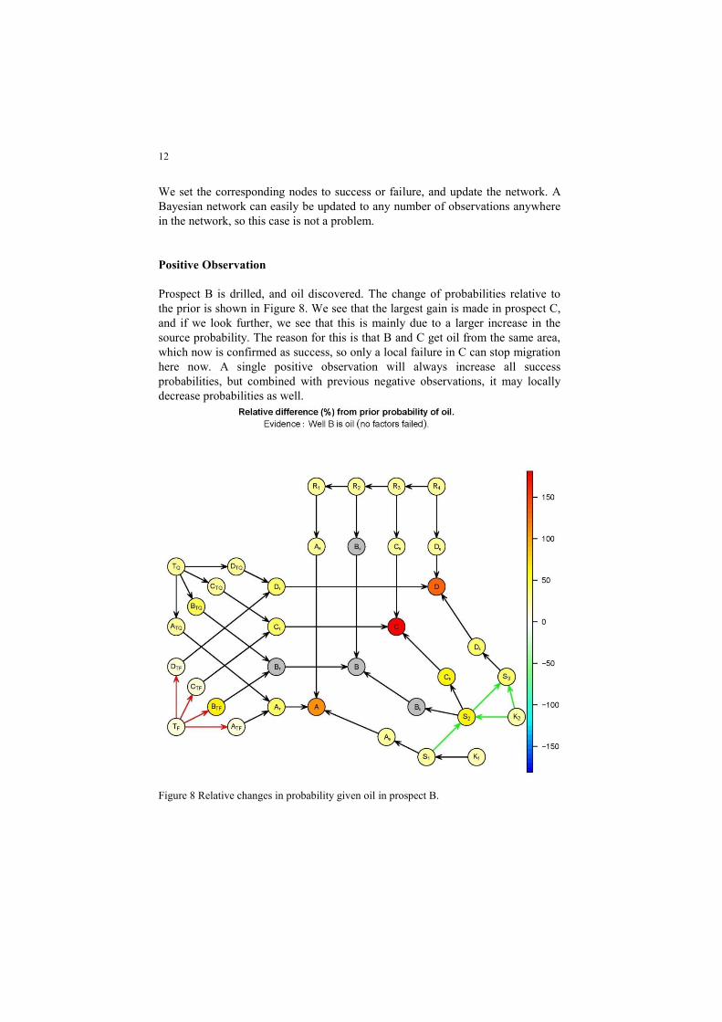
Prospect B is drilled, and oil discovered. The change of probabilities relative to

the prior is shown in Figure 8. We see that the largest gain is made in prospect C,

and if we look further, we see that this is mainly due to a larger increase in the

source probability. The reason for this is that B and C get oil from the same area,

which now is confirmed as success, so only a local failure in C can stop migration

here now. A single positive observation will always increase all success

probabilities, but combined with previous negative observations, it may locally

decrease probabilities as well.

Figure 8 Relative changes in probability given oil in prospect B.

13

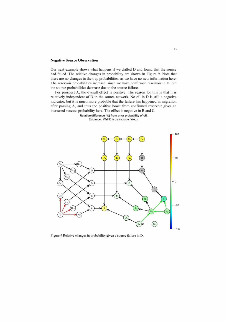
Negative Source Observation

Our next example shows what happens if we drilled D and found that the source

had failed. The relative changes in probability are shown in Figure 9. Note that

there are no changes in the trap probabilities, as we have no new information here.

The reservoir probabilities increase, since we have confirmed reservoir in D, but

the source probabilities decrease due to the source failure.

For prospect A, the overall effect is positive. The reason for this is that it is

relatively independent of D in the source network. No oil in D is still a negative

indicator, but it is much more probable that the failure has happened in migration

after passing A, and thus the positive boost from confirmed reservoir gives an

increased success probability here. The effect is negative in B and C.

Figure 9 Relative changes in probability given a source failure in D.

14

Concluding Remarks

Bayesian networks seem to be a great tool for modeling prospect dependencies.

They are flexible enough to handle different kinds of geological correlations, yet

simple enough to keep the number of parameters low. The parameters are all in

the form of conditional probabilities, which exploration geologists are familiar

with. Adding observations to a Bayesian network is simple, and they are

computationally efficient. The main challenge lies in the process of building the

network, which currently requires close cooperation between geologists and

statisticians

Bibliography

[1] J. E. Bickel, J. E. Smith and J. L. Meyer, "Modeling Dependence

Among Geologic Risks in Sequential Exploration Decisions," SPE

Reservoir Evaluation & Engineering, no. 11, 2008.

[2] J. D. V. Wees, H. Mijnleff, J. Lutgert, J. Breunese, C. Bos, P.

Rosenkranz and F. Neele, "A Bayesian Belief Network Approach for

Assessing the Impact of Exploration Prospect Interdependency: An

Application to Predict gas Discoveries in the Netherlands," AAPG

Bulletin, vol. 92, no. 10, 2008.

[3] G. Martinelli, J. Eidsvik, R. Hauge and M. D. Førland, "Bayesian

networks for prospect analysis in the North Sea," AAPG Bulletin, vol. 95,

no. 8, 2011.

[4] M. Stien, M. Drange-Espeland and R. Hauge, "On using Bayesian

netwroks for modeling dependencies between prospects in oil

exploration," in IAMG, 2011.

[5] R. G. Cowell, A. P. Dawid, S. L. Lauritzen og D. J. Spiegelhalter,

Probabilisitc networks and expert systems, Springer series in Information

Science and Statistics, 2007.