Modeling and Solving Constraints

Erin CattoBlizzard Entertainment

Basic Idea

Constraints are used to simulate joints, contact, and collision.We need to solve the constraints to stack boxes and to keep ragdoll limbs attached.Constraint solvers do this by calculating impulse or forces, and applying them to the constrained bodies.

OverviewConstraint Formulas

Jacobians, Lagrange MultipliersModeling Constraints

Joints, Motors, ContactBuilding a Constraint Solver

Sequential Impulses

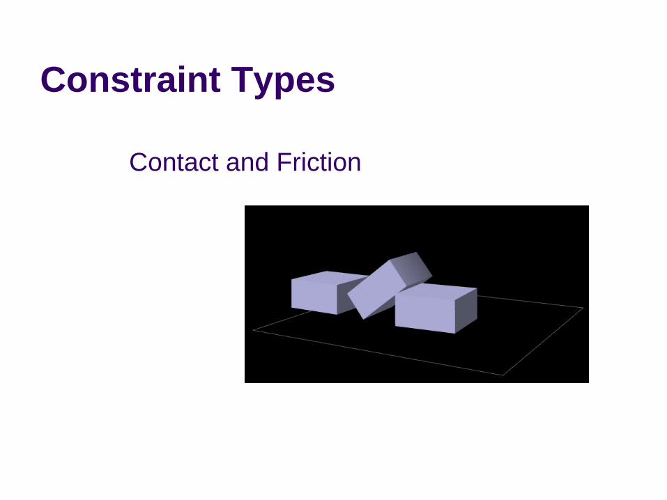
Constraint Types

Contact and Friction

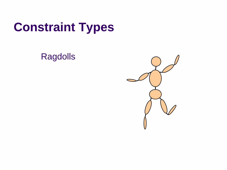
Constraint Types

Ragdolls

Constraint Types

Particles and Cloth

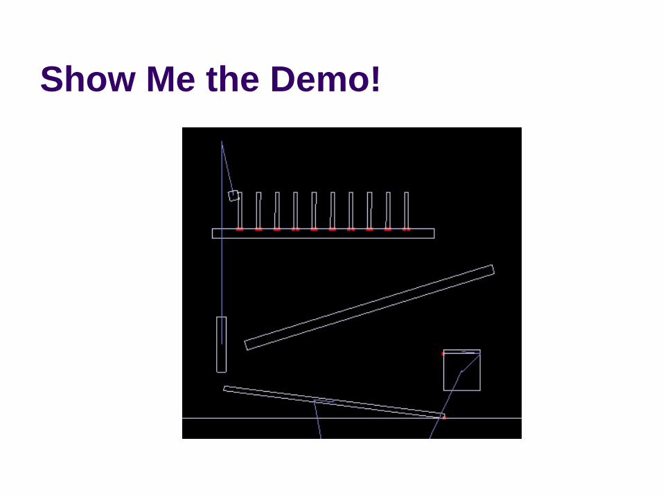
Show Me the Demo!

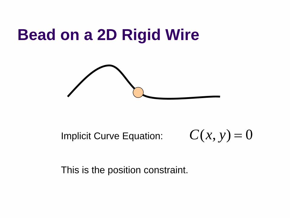
Bead on a 2D Rigid Wire

( , ) 0C x y =Implicit Curve Equation:

This is the position constraint.

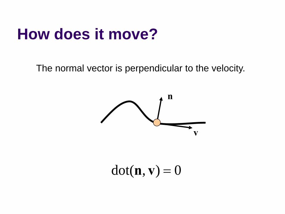
How does it move?

v

The normal vector is perpendicular to the velocity.

n

dot( , ) 0=n v

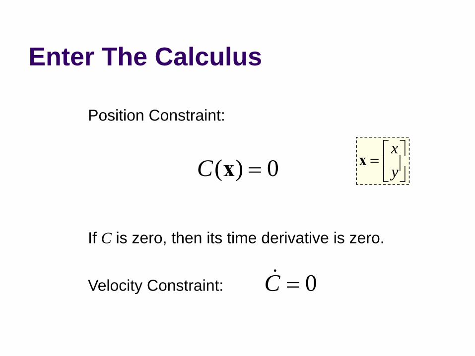
Enter The Calculus

( ) 0C =x

Position Constraint:

0C =&Velocity Constraint:

If C is zero, then its time derivative is zero.

xy⎡ ⎤

= ⎢ ⎥⎣ ⎦

x

Velocity Constraint

Velocity constraints define the allowed motion.Next we’ll show that velocity constraints depend linearly on velocity.

0C =&

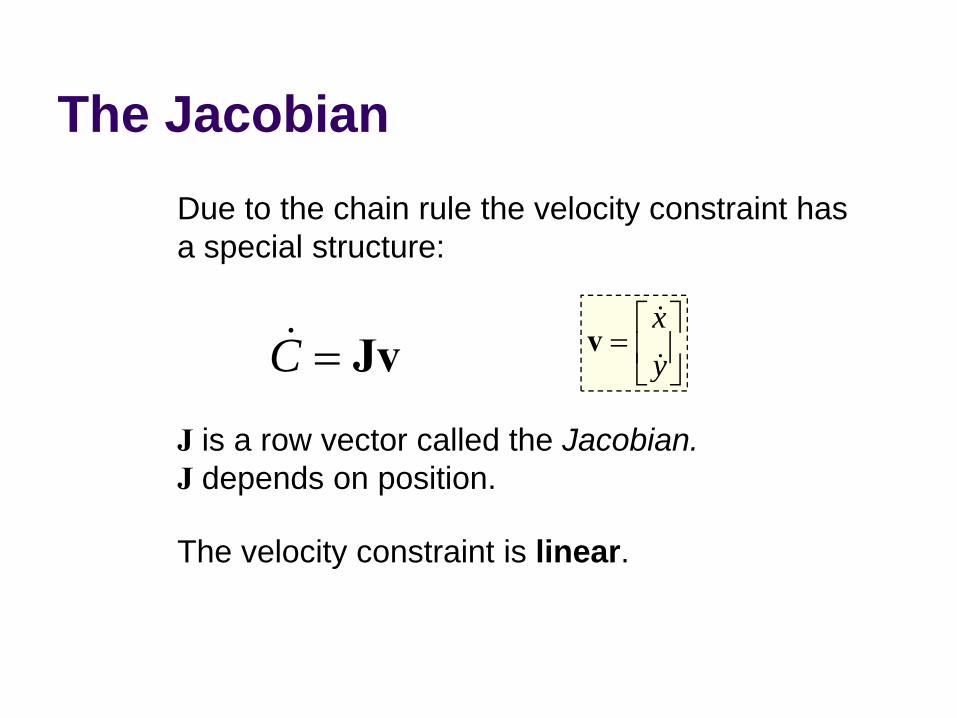
The JacobianDue to the chain rule the velocity constraint has a special structure:

C = Jv&

J is a row vector called the Jacobian.J depends on position.

xy⎡ ⎤

= ⎢ ⎥⎣ ⎦

v&

&

The velocity constraint is linear.

The Jacobian

v

TJ

The Jacobian is perpendicular to the velocity.

0C = =Jv&

Constraint Force

v

Assume the wire is frictionless.

What is the force between the wire and the bead?

Lagrange Multiplier

v

cF

Intuitively the constraint force Fc is parallel to the normal vector.

Tc λ=F J

Direction known.Magnitude unknown. implies

Lagrange MultiplierThe Lagrange Multiplier (lambda) is the constraint force signed magnitude.We use a constraint solver to compute lambda.More on this later.

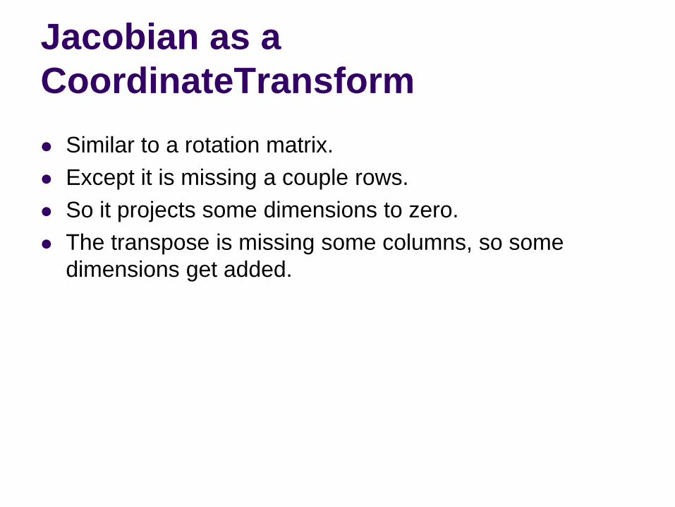
Jacobian as a CoordinateTransform

Similar to a rotation matrix.Except it is missing a couple rows.So it projects some dimensions to zero.The transpose is missing some columns, so some dimensions get added.

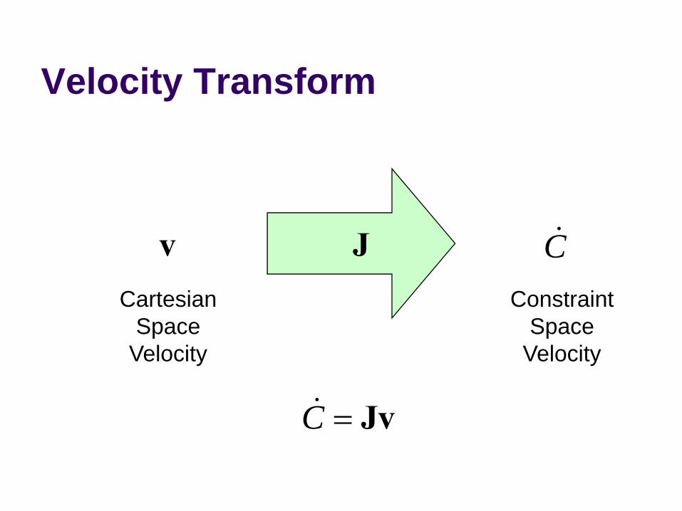
Velocity Transform

v J C&

CartesianSpace

Velocity

ConstraintSpace

Velocity

C = Jv&

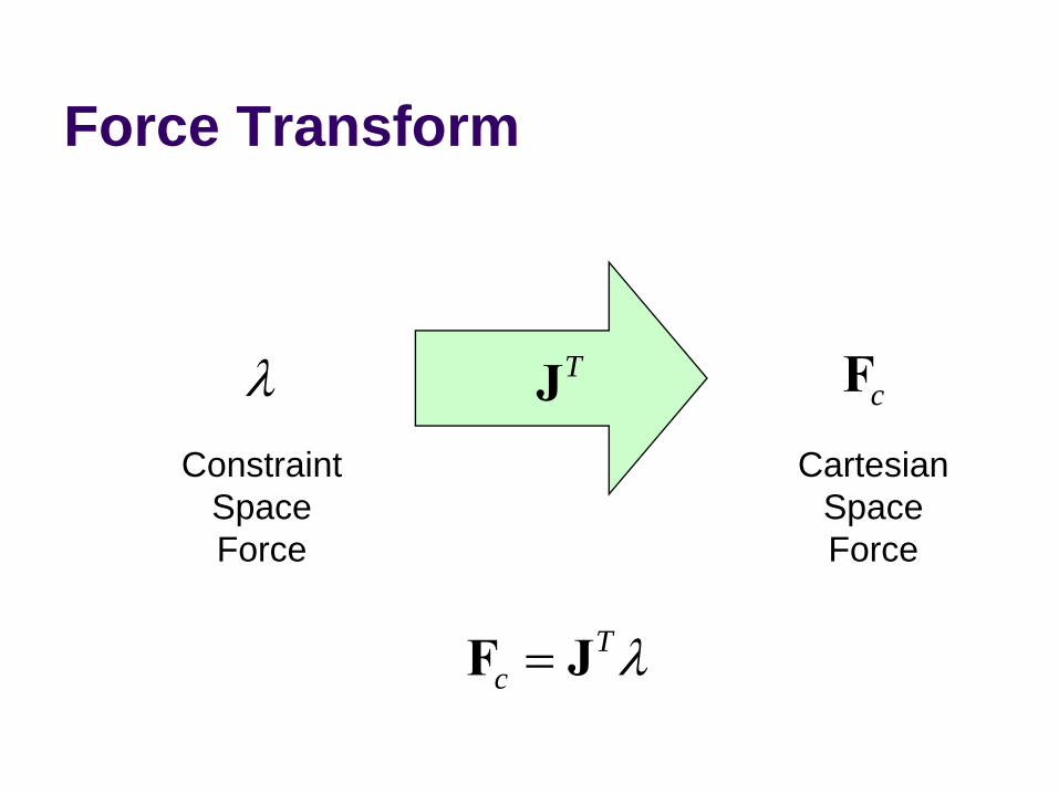
Force Transform

cFConstraint

SpaceForce

CartesianSpaceForce

λ TJ

Tc λ=F J

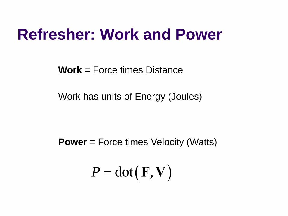
Refresher: Work and Power

Work = Force times Distance

Work has units of Energy (Joules)

Power = Force times Velocity (Watts)

( )dot ,P = F V

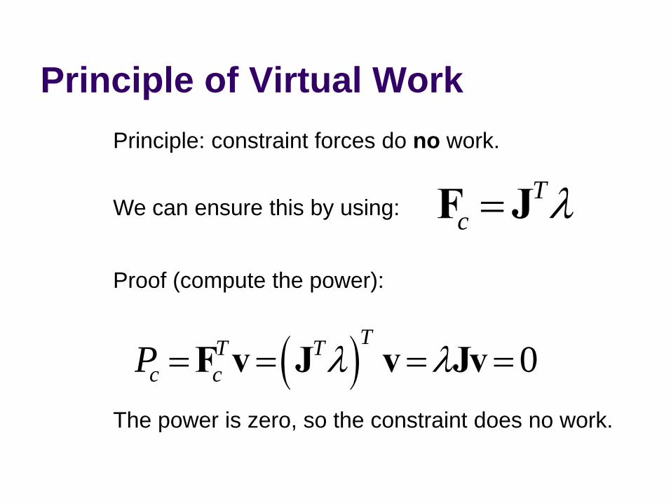
Principle of Virtual Work

Tc λ=F J

Principle: constraint forces do no work.

( ) 0TT T

c cP λ λ= = = =F v J v Jv

Proof (compute the power):

The power is zero, so the constraint does no work.

We can ensure this by using:

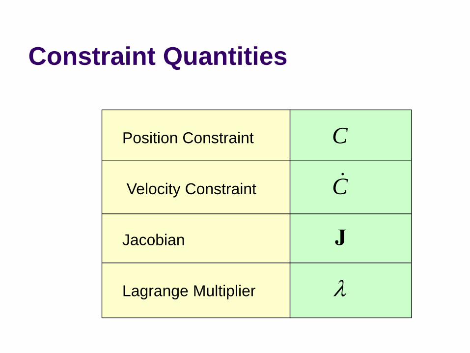
Constraint Quantities

C

C&

J

λ

Position Constraint

Velocity Constraint

Jacobian

Lagrange Multiplier

Why all the Painful Abstraction?

We want to put all constraints into a common form for the solver.This allows us to efficiently try different solution techniques.

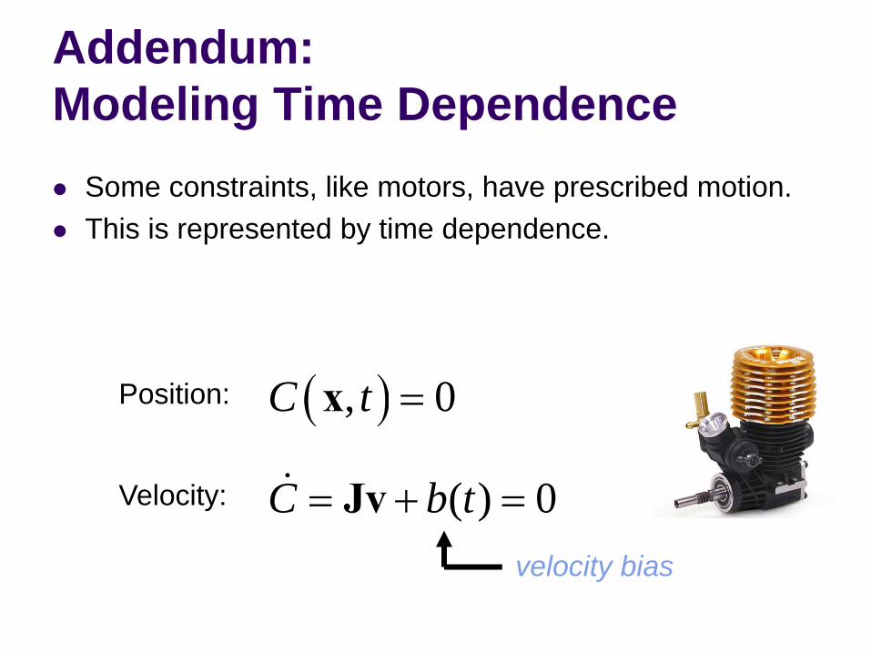
Addendum:Modeling Time Dependence

Some constraints, like motors, have prescribed motion.This is represented by time dependence.

( ), 0C t =x

( ) 0C b t= + =Jv&

Position:

Velocity:

velocity bias

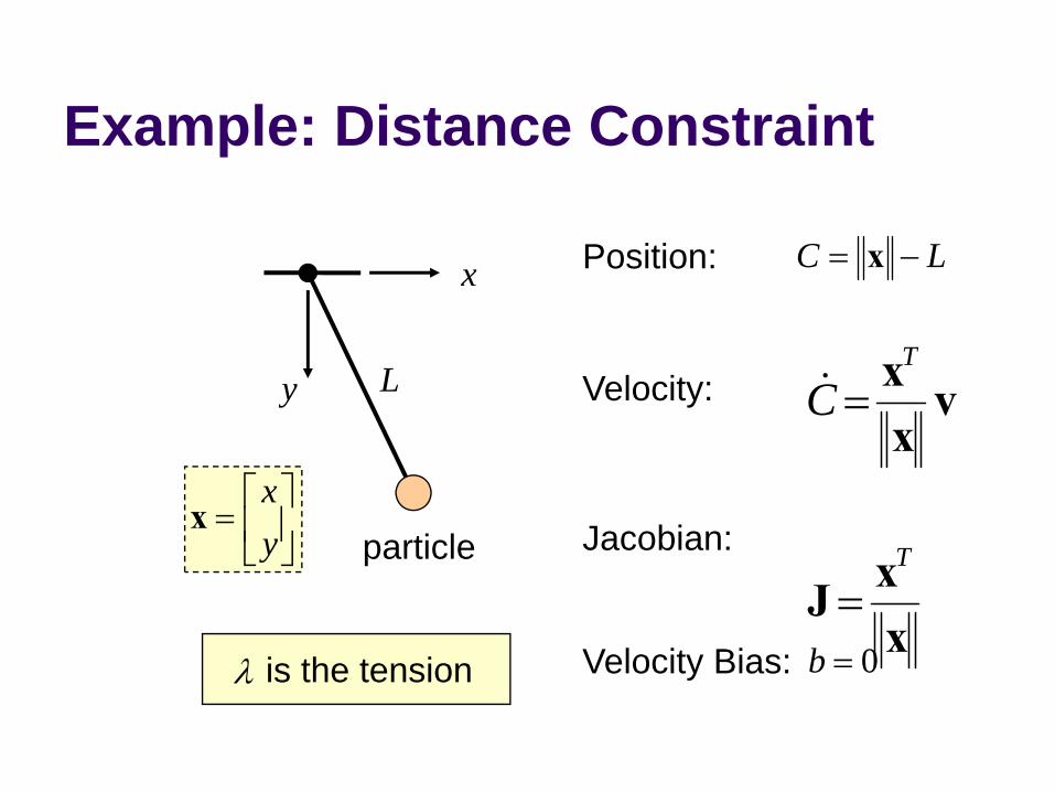
Example: Distance Constraint

T

C =x vx

&

T

=xJx

y

x

L

C L= −x

0b =

Position:

Velocity:

Jacobian:

Velocity Bias:λ is the tension

particlexy⎡ ⎤

= ⎢ ⎥⎣ ⎦

x

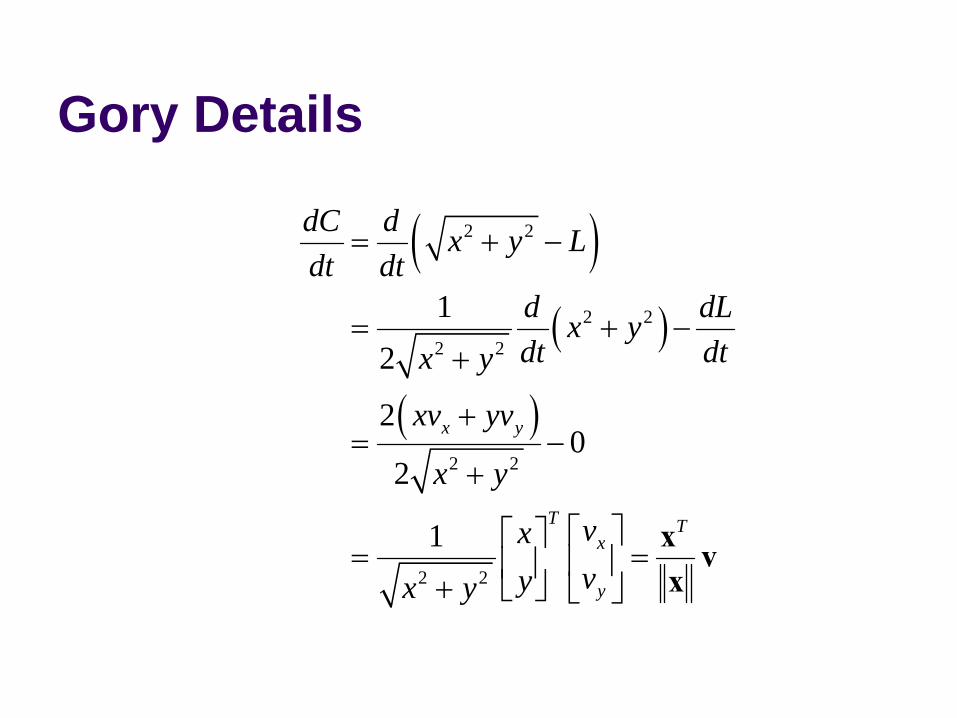
Gory Details

( )( )

( )

2 2

2 2

2 2

2 2

2 2

12

20

2

1

x y

T Tx

y

dC d x y Ldt dt

d dLx ydt dtx y

xv yv

x y

vxvyx y

= + −

= + −+

+= −

+

⎡ ⎤⎡ ⎤= =⎢ ⎥⎢ ⎥

+ ⎣ ⎦ ⎣ ⎦

x vx

Computing the JacobianAt first, it is not easy to compute the Jacobian.It gets easier with practice.If you can define a position constraint, you can find its Jacobian.Here’s how …

A Recipe for JUse geometry to write C.Differentiate C with respect to time.Isolate v.Identify J and b by inspection.

C b= +Jv&

Constraint PotpourriJointsMotorsContactRestitutionFriction

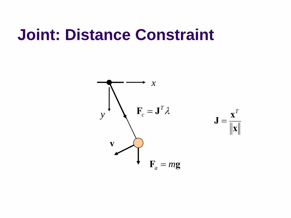
Joint: Distance Constraint

Tc λ=F Jy

x

v

a m=F g

T

=xJx

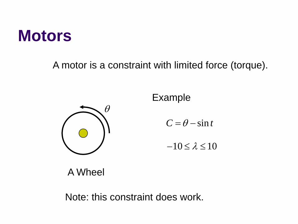
MotorsA motor is a constraint with limited force (torque).

θsinC tθ= −

Example

10 10λ− ≤ ≤

A Wheel

Note: this constraint does work.

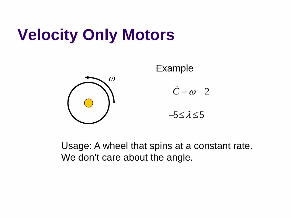
Velocity Only Motors

ω2C ω= −&

Example

Usage: A wheel that spins at a constant rate.We don’t care about the angle.

5 5λ− ≤ ≤

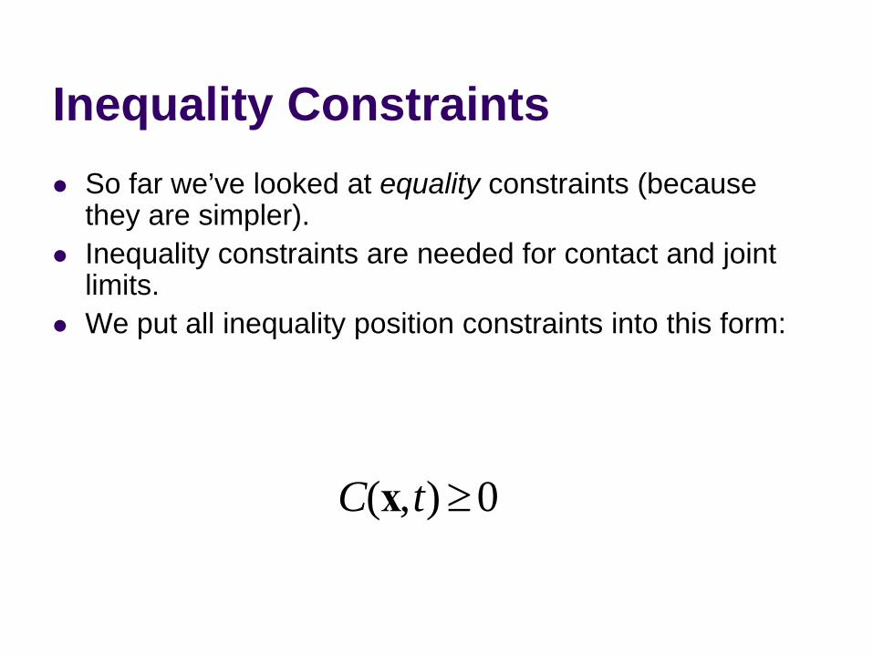
Inequality ConstraintsSo far we’ve looked at equality constraints (because they are simpler).Inequality constraints are needed for contact and joint limits.We put all inequality position constraints into this form:

( , ) 0C t ≥x

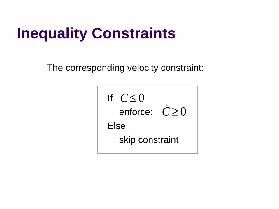
Inequality Constraints

0C≤

The corresponding velocity constraint:

If0C≥&

Elseskip constraint

enforce:

Inequality Constraints

Force Limits:

Inequality constraints don’t suck.

0 λ≤ ≤ ∞

Contact ConstraintNon-penetration.Restitution: bounceFriction: sliding, sticking, and rolling

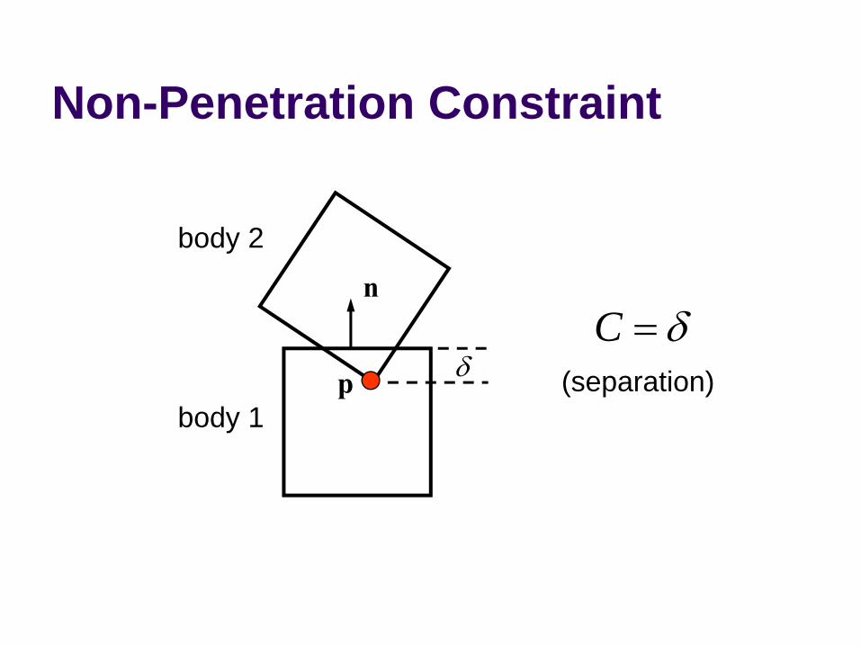
Non-Penetration Constraint

δ

nC δ=

p

body 2

body 1(separation)

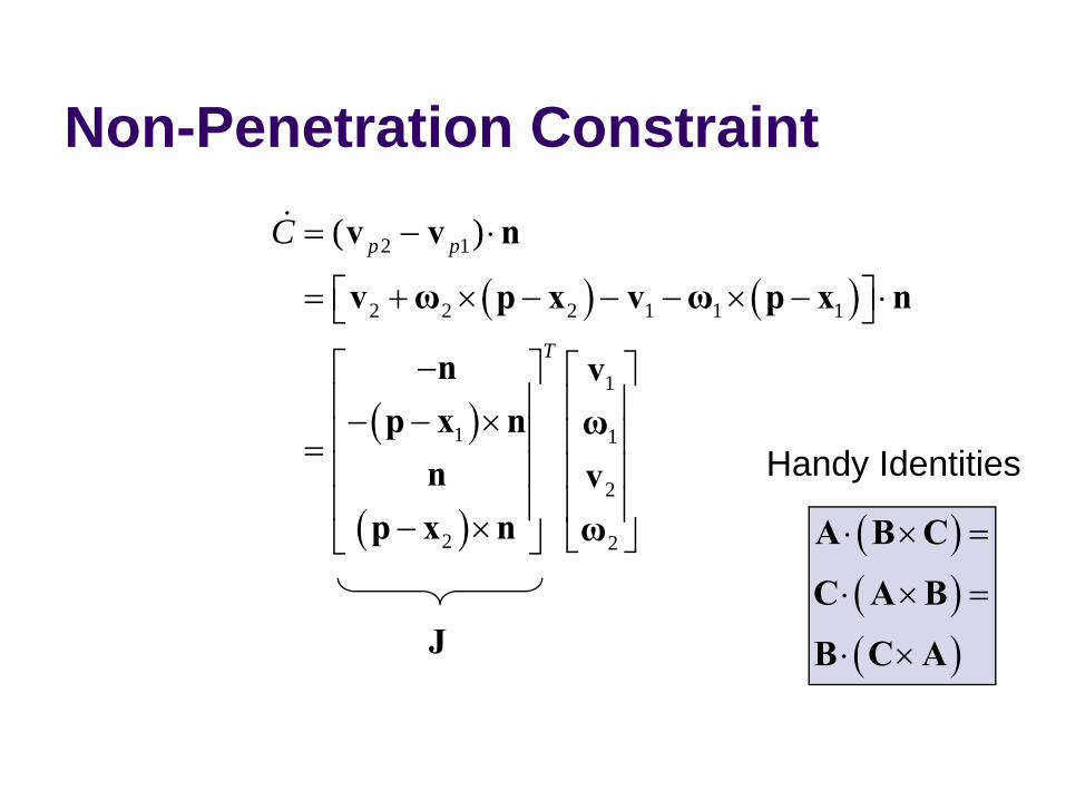
Non-Penetration Constraint

( ) ( )

( )

( )

2 1

2 2 2 1 1 1

1

1 1

2

2 2

( )p p

T

C = − ⋅

⎡ ⎤= + × − − − × − ⋅⎣ ⎦

−⎡ ⎤ ⎡ ⎤⎢ ⎥ ⎢ ⎥− − ×⎢ ⎥ ⎢ ⎥=⎢ ⎥ ⎢ ⎥⎢ ⎥ ⎢ ⎥− × ⎣ ⎦⎣ ⎦

v v n

v ω p x v ω p x n

n vp x n ωn v

p x n ω

&

J

( )( )( )

⋅ × =

⋅ × =

⋅ ×

A B C

C A B

B C A

Handy Identities

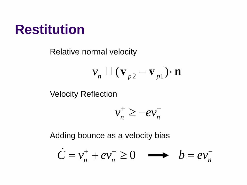
Restitution

2 1( )n p pv − ⋅v v n

Relative normal velocity

Adding bounce as a velocity bias

nb ev−=0n nC v ev+ −= + ≥&

n nv ev+ −≥ −

Velocity Reflection

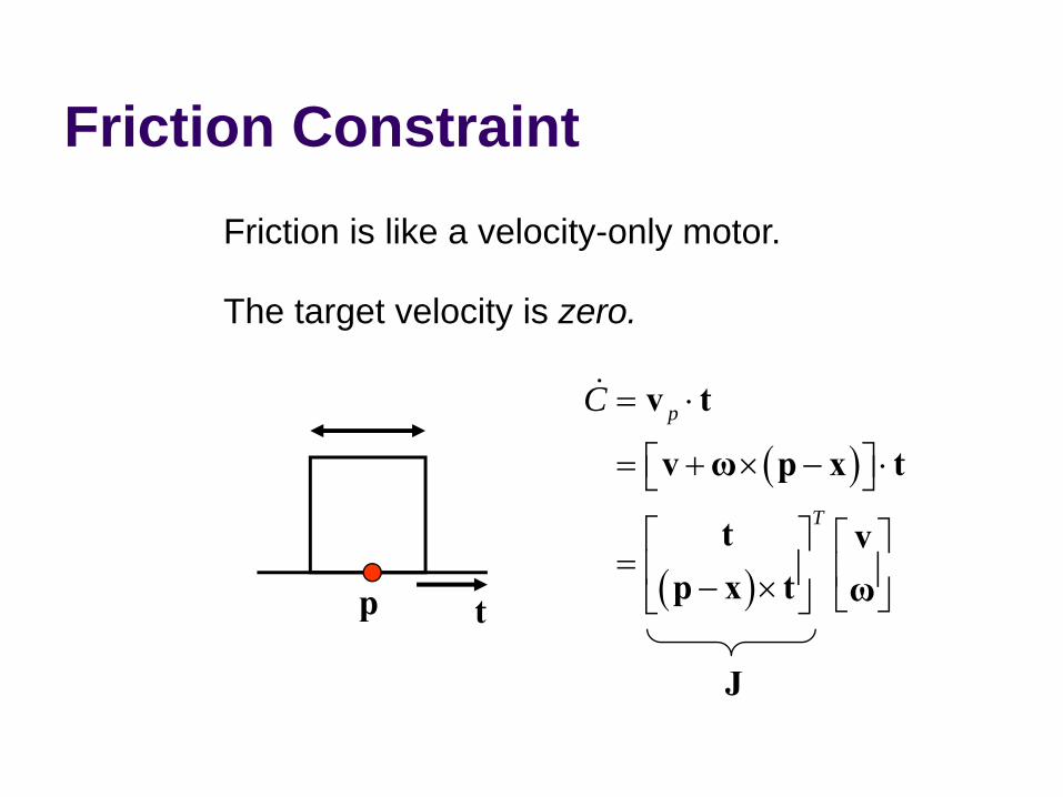
Friction ConstraintFriction is like a velocity-only motor.

The target velocity is zero.

p

( )

( )

p

T

C = ⋅

⎡ ⎤= + × − ⋅⎣ ⎦

⎡ ⎤ ⎡ ⎤= ⎢ ⎥ ⎢ ⎥− × ⎣ ⎦⎣ ⎦

v t

v ω p x t

t vp x t ω

&

J

t

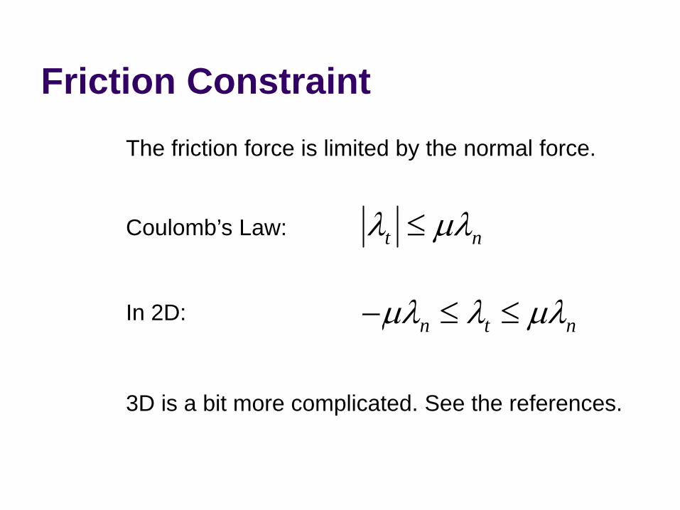
Friction ConstraintThe friction force is limited by the normal force.

Coulomb’s Law: t nλ μλ≤

In 2D: n t nμλ λ μλ− ≤ ≤

3D is a bit more complicated. See the references.

Constraints SolversWe have a bunch of constraints.We have unknown constraint forces.We need to solve for these constraint forces.There are many ways different ways to compute constraint forces.

Constraint Solver TypesGlobal Solvers (slow)Iterative Solvers (fast)

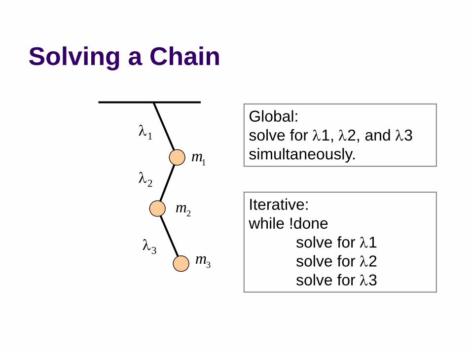
Solving a Chain

λ1

λ2

λ3

Global:solve for λ1, λ2, and λ3 simultaneously.

Iterative:while !done

solve for λ1solve for λ2solve for λ3

1m

2m

3m

Sequential Impulses (SI)An iterative solver.SI applies impulses at each constraint to correct the velocity error.SI is fast and stable.Converges to a global solution.

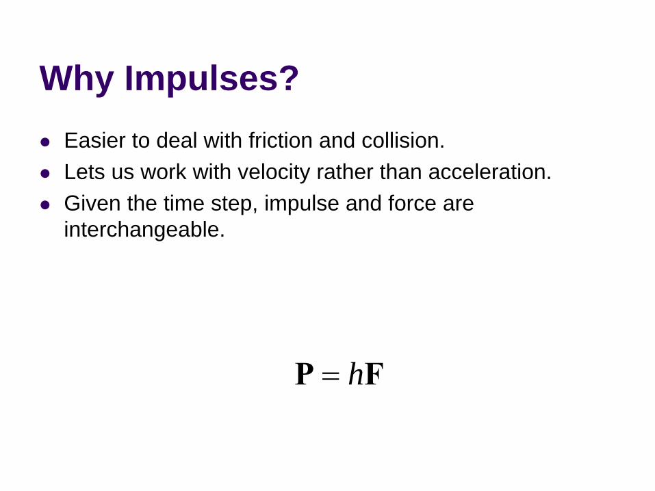
Why Impulses?Easier to deal with friction and collision.Lets us work with velocity rather than acceleration.Given the time step, impulse and force are interchangeable.

h=P F

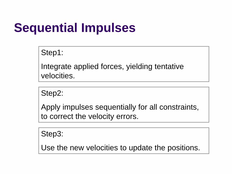
Sequential Impulses

Step1:

Integrate applied forces, yielding tentative velocities.

Step2:

Apply impulses sequentially for all constraints, to correct the velocity errors.

Step3:

Use the new velocities to update the positions.

Step 1: Newton’s Law

a c= +Mv F F&

We separate applied forces andconstraint forces.

mass matrix

Step 1: Mass Matrix

0 00 00 0

mm

m

⎡ ⎤⎢ ⎥= ⎢ ⎥⎢ ⎥⎣ ⎦

MParticle

Rigid Body m⎡ ⎤= ⎢ ⎥⎣ ⎦

E 0M

0 I

May involve multiple particles/bodies.

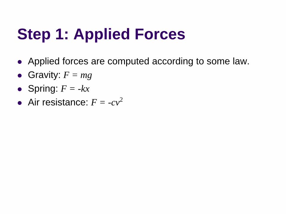
Step 1: Applied ForcesApplied forces are computed according to some law.Gravity: F = mgSpring: F = -kxAir resistance: F = -cv2

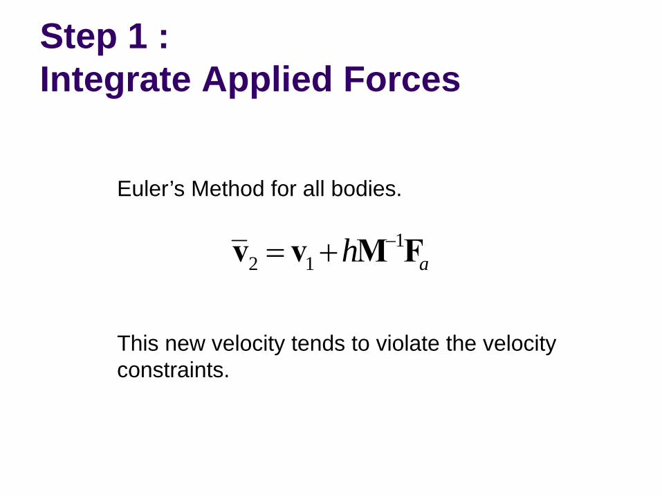
Step 1 :Integrate Applied Forces

12 1 ah −= +v v M F

Euler’s Method for all bodies.

This new velocity tends to violate the velocity constraints.

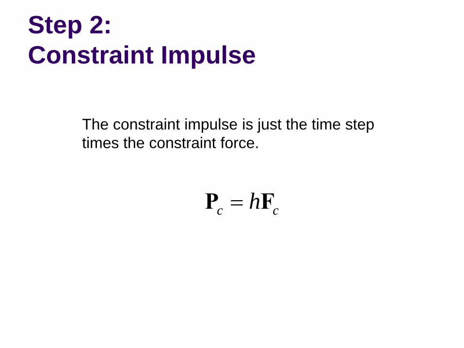
Step 2:Constraint Impulse

The constraint impulse is just the time step times the constraint force.

c ch=P F

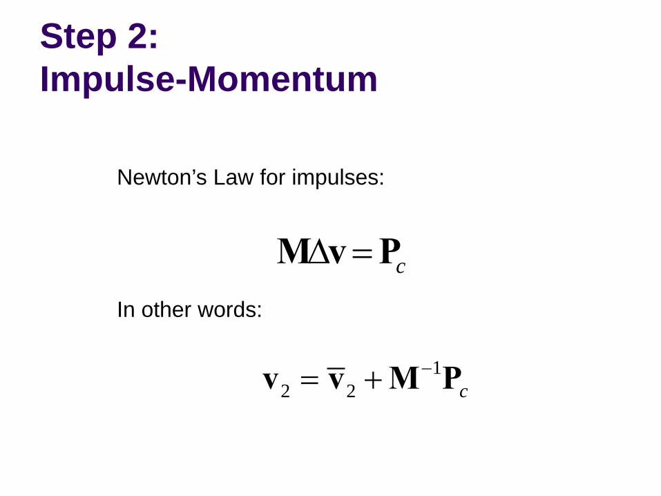
Step 2:Impulse-Momentum

Newton’s Law for impulses:

cΔ =M v PIn other words:

12 2 c

−= +v v M P

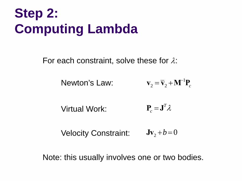
Step 2:Computing Lambda

For each constraint, solve these for λ:

12 2

2 0

c

Tc

b

λ

−= +

=

+ =

v v M P

P J

Jv

Newton’s Law:

Virtual Work:

Velocity Constraint:

Note: this usually involves one or two bodies.

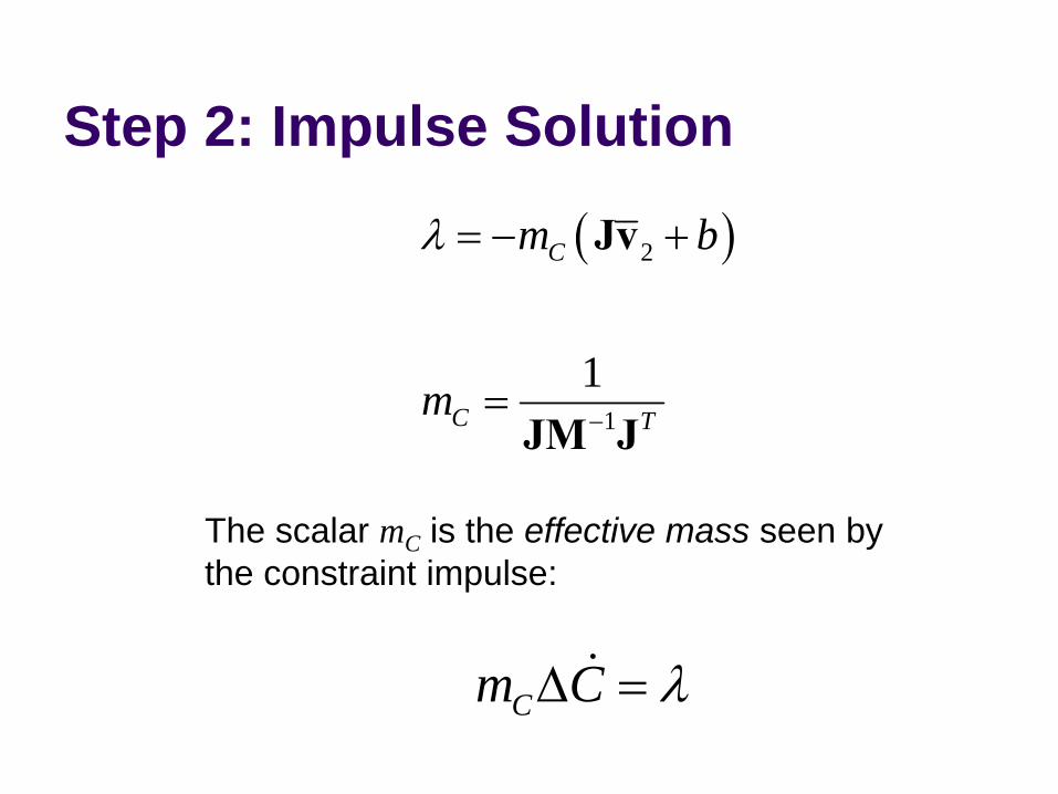
Step 2: Impulse Solution

( )2

1

1

C

C T

m b

m

λ

−

= − +

=

Jv

JM J

The scalar mC is the effective mass seen bythe constraint impulse:

Cm C λΔ =&

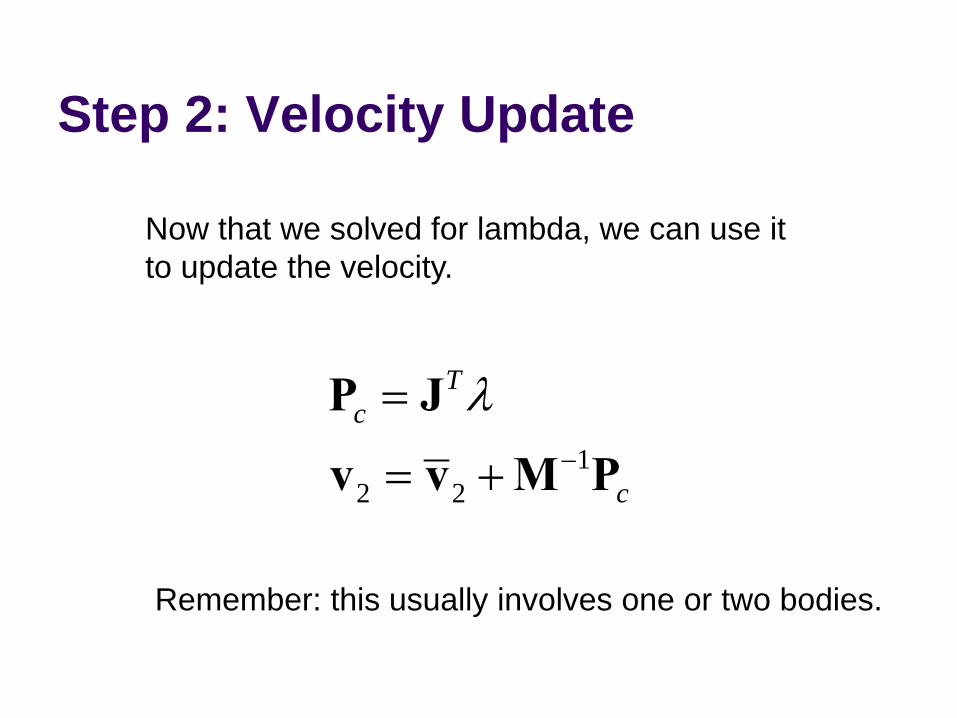
Step 2: Velocity Update

12 2

Tc

c

λ−

=

= +

P J

v v M P

Now that we solved for lambda, we can use itto update the velocity.

Remember: this usually involves one or two bodies.

Step 2: IterationLoop over all constraints until you are done:

- Fixed number of iterations.- Corrective impulses become small.- Velocity errors become small.

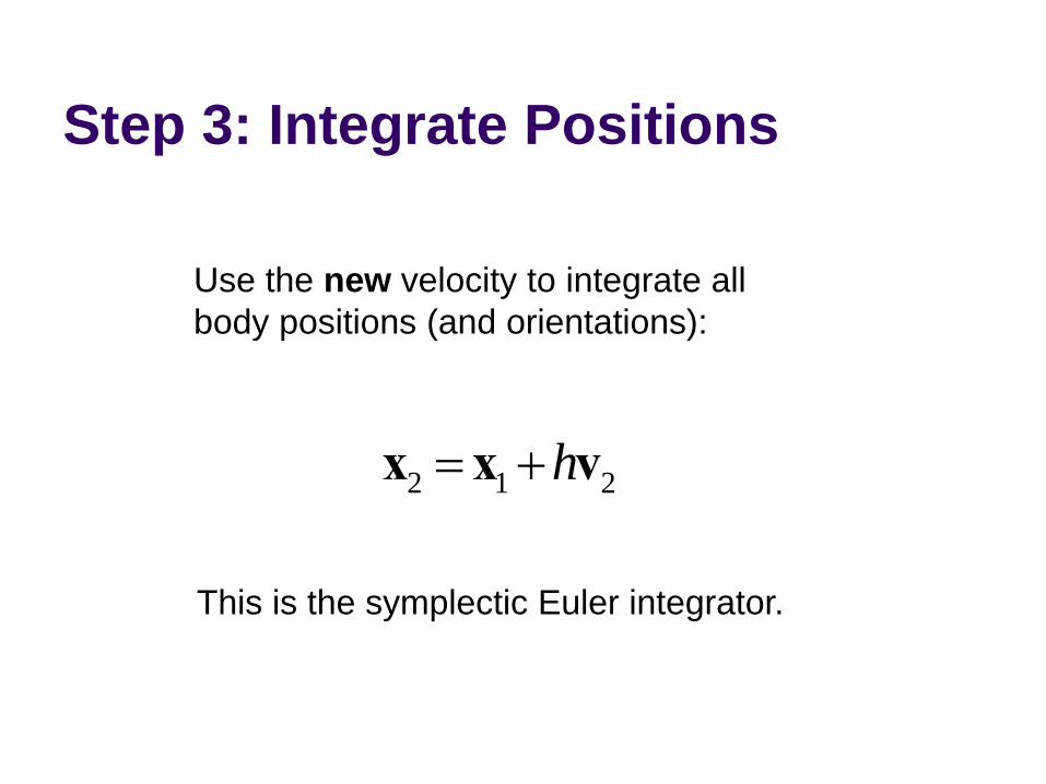
Step 3: Integrate Positions

2 1 2h= +x x v

Use the new velocity to integrate all body positions (and orientations):

This is the symplectic Euler integrator.

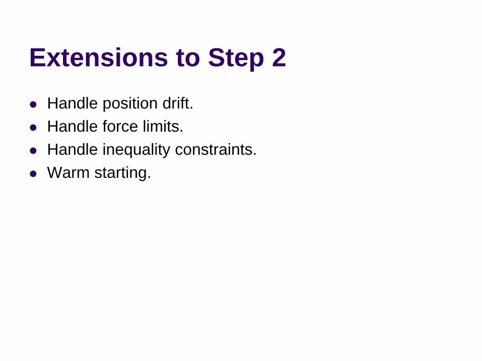
Extensions to Step 2Handle position drift.Handle force limits.Handle inequality constraints.Warm starting.

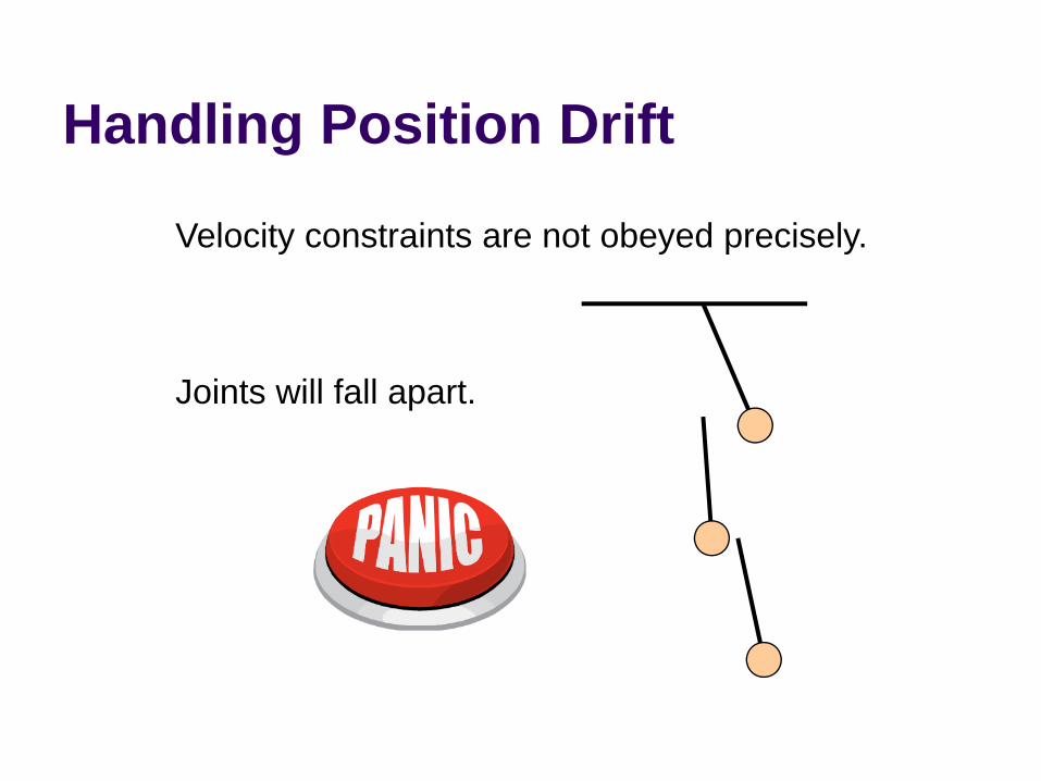
Handling Position Drift

Velocity constraints are not obeyed precisely.

Joints will fall apart.

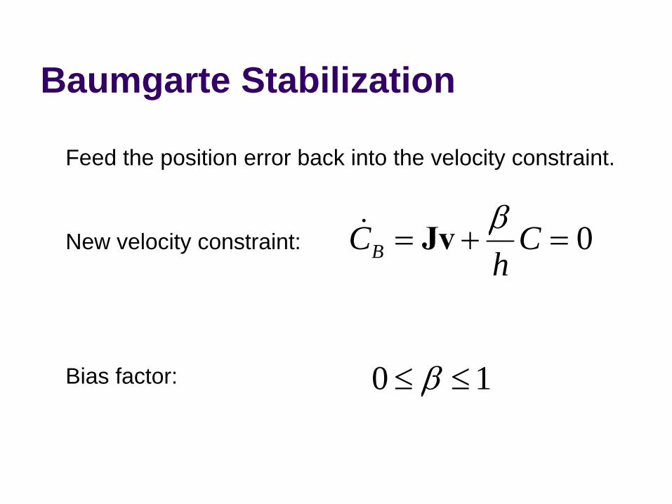
Baumgarte Stabilization

Feed the position error back into the velocity constraint.

0BC Chβ

= + =Jv&New velocity constraint:

Bias factor: 0 1β≤ ≤

Baumgarte Stabilization

What is the solution to this?

0C Chβ

+ =&

First-order differential equation …

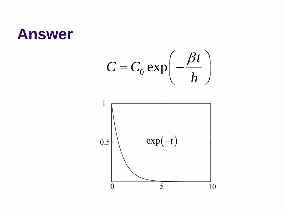
Answer

0 exp tC Chβ⎛ ⎞= −⎜ ⎟

⎝ ⎠

( )exp t−

Tuning the Bias FactorIf your simulation has instabilities, set the bias factor to zero and check the stability.Increase the bias factor slowly until the simulation becomes unstable.Use half of that value.

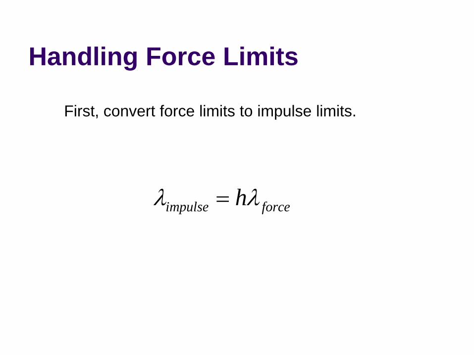
Handling Force Limits

First, convert force limits to impulse limits.

impulse forcehλ λ=

Handling Impulse Limits

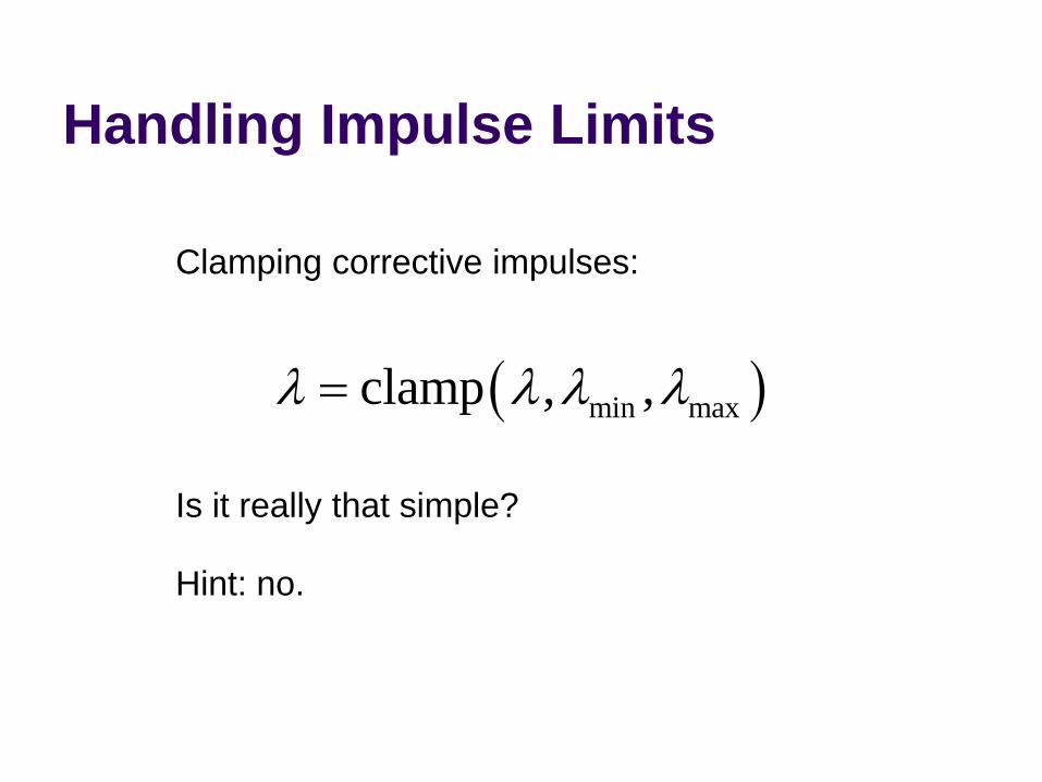
Clamping corrective impulses:

( )min maxclamp , ,λ λ λ λ=

Is it really that simple?

Hint: no.

How to ClampEach iteration computes corrective impulses.Clamping corrective impulses is wrong!You should clamp the total impulse applied over the time step.The following example shows why.

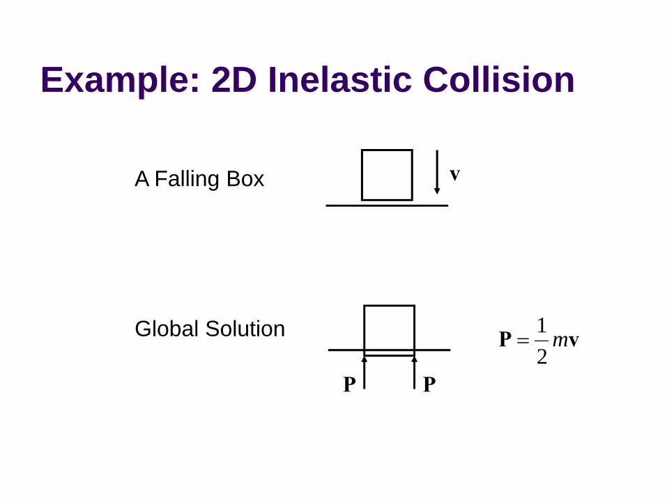
Example: 2D Inelastic Collision

v

P

A Falling Box

P

Global Solution 12

m=P v

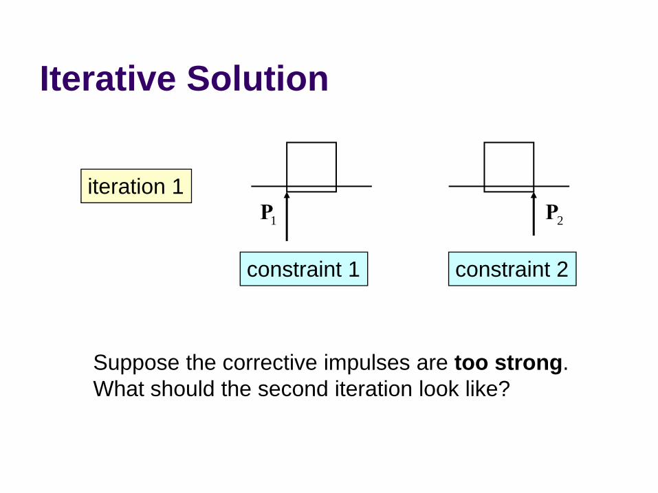
Iterative Solution

1P 2Piteration 1

constraint 1 constraint 2

Suppose the corrective impulses are too strong.What should the second iteration look like?

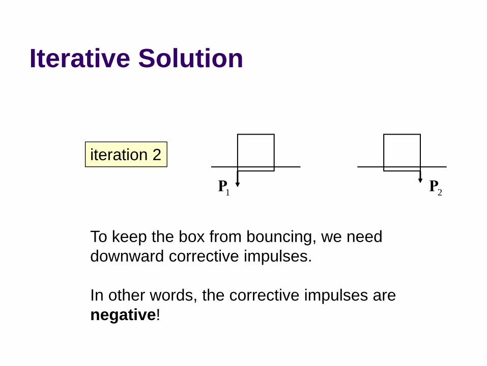
Iterative Solution

1P 2P

iteration 2

To keep the box from bouncing, we needdownward corrective impulses.

In other words, the corrective impulses arenegative!

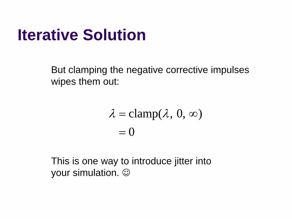
Iterative Solution

But clamping the negative corrective impulseswipes them out:

clamp( , 0, )0

λ λ= ∞=

This is one way to introduce jitter intoyour simulation. ☺

Accumulated ImpulsesFor each constraint, keep track of the total impulse applied.This is the accumulated impulse.Clamp the accumulated impulse.This allows the corrective impulse to be negative yet the accumulated impulse is still positive.

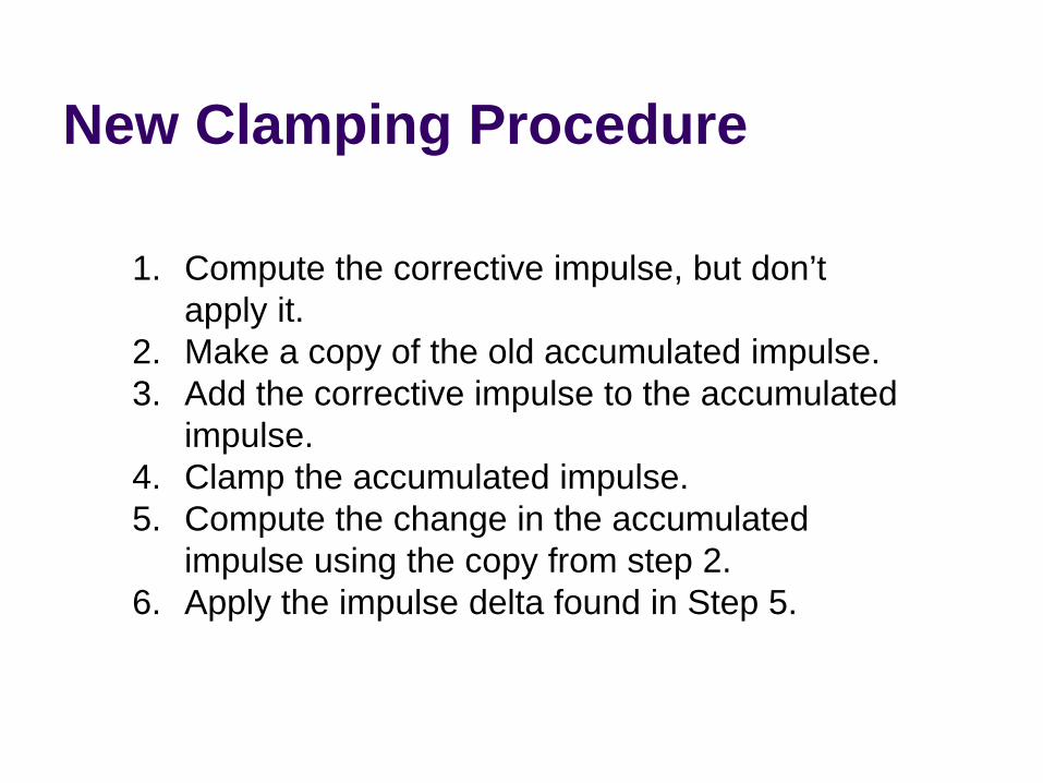
New Clamping Procedure

1. Compute the corrective impulse, but don’t apply it.

2. Make a copy of the old accumulated impulse.3. Add the corrective impulse to the accumulated

impulse.4. Clamp the accumulated impulse.5. Compute the change in the accumulated

impulse using the copy from step 2.6. Apply the impulse delta found in Step 5.

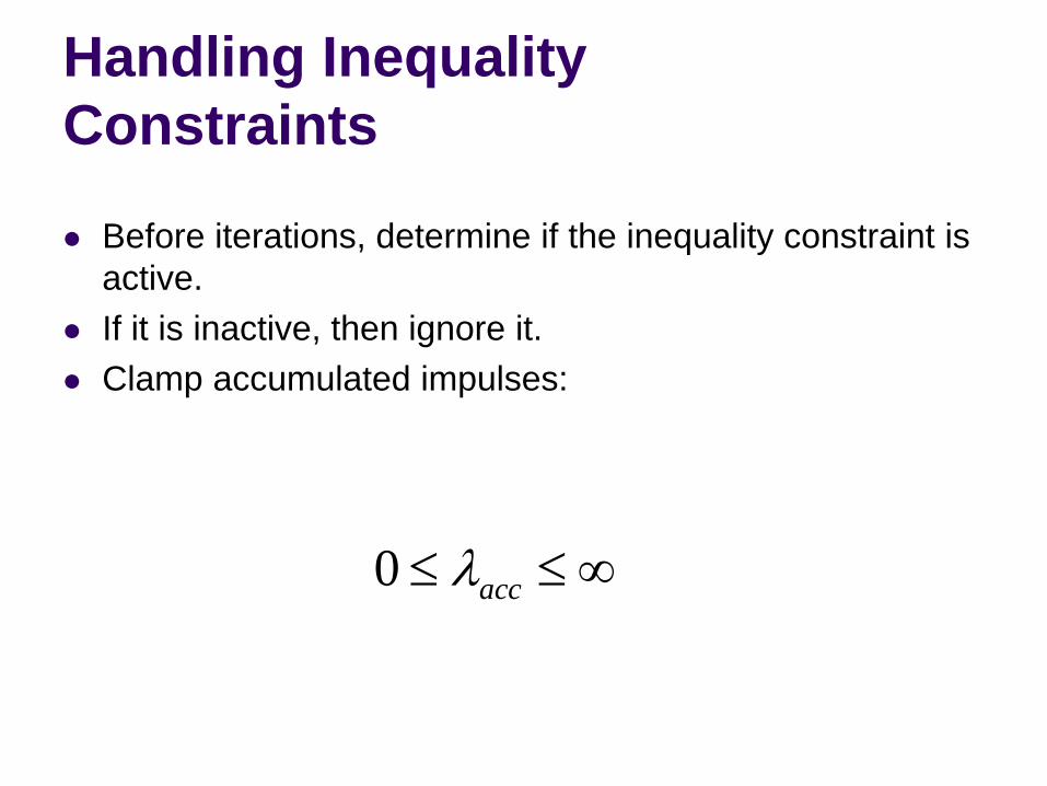
Handling Inequality Constraints

Before iterations, determine if the inequality constraint is active.If it is inactive, then ignore it.Clamp accumulated impulses:

0 accλ≤ ≤ ∞

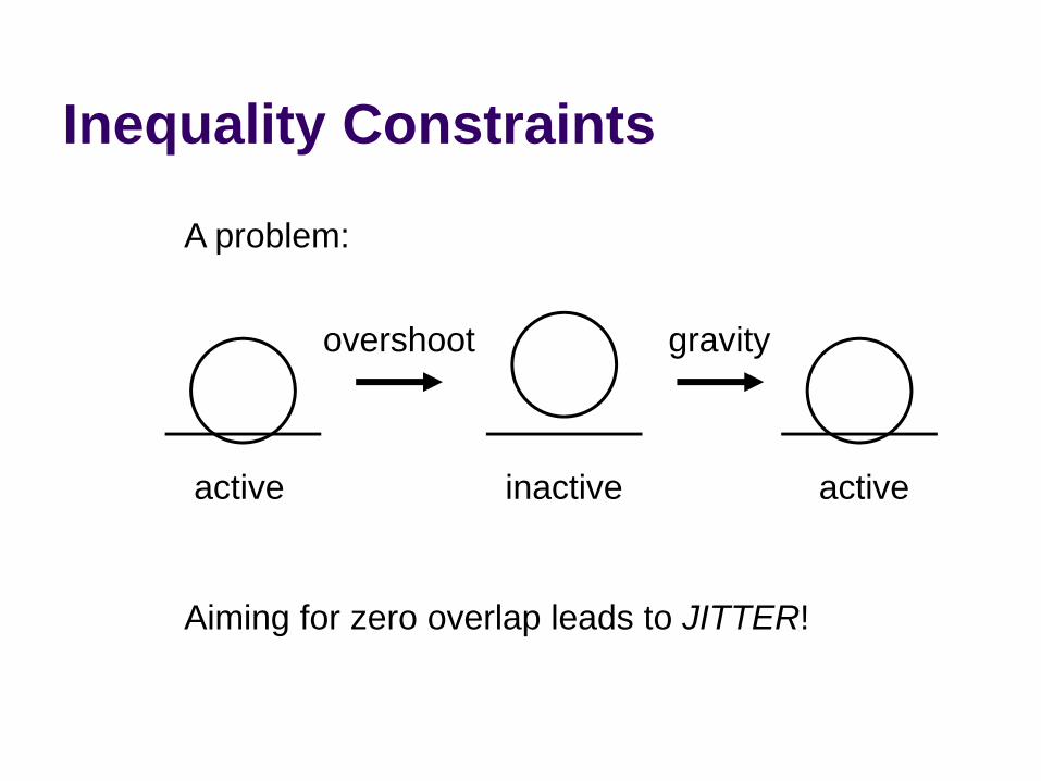
Inequality Constraints

A problem:

overshoot

active inactive active

gravity

Aiming for zero overlap leads to JITTER!

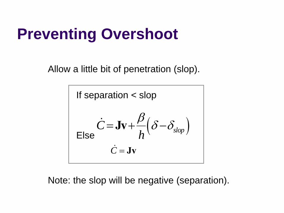
Preventing Overshoot

( )slopChβ δ δ= + −Jv&

Allow a little bit of penetration (slop).

If separation < slop

C = Jv&

Else

Note: the slop will be negative (separation).

Warm StartingIterative solvers use an initial guess for the lambdas.So save the lambdas from the previous time step.Use the stored lambdas as the initial guess for the new step.Benefit: improved stacking.

Step 1.5Apply the stored impulses.Use the stored impulses to initialize the accumulated impulses.

Step 2.5Store the accumulated impulses.

Further Reading &Sample Code

http://www.gphysics.com/downloads/

Box2DAn open source 2D physics engine.http://www.box2d.orgWritten in C++.