modeling and simulation for physical vapor deposition
TRANSCRIPT

Modeling and Simulation for Physical Vapor
Deposition: Multiscale Model
Jurgen Geiser and Robert Rohle
Humboldt-Universitat zu Berlin,Department of Mathematics,
Unter den Linden 6, D-10099 Berlin, [email protected]
Abstract. In this paper, we present modeling and simulation for phys-ical vapor deposition for metallic bipolar plates.In the models, we discuss the application of different models to simulatethe transport of chemical reactions of the gas species in the gas-chamber.The so called sputter process is an extremely sensitive process to depositthin layers to metallic plates.
We taken into account lower order models to obtain first results withrespect to the gas fluxes and the kinetics in the chamber.The model equations can be treated analytically in some circumstancesand complicate multi-dimensional models are solved numerically with asoftware-packages (UG unstructed grids, see [2]).Because of multi-scaling and multi-physical behavior of the models, wediscuss adapted schemes to solve more accurate in the different domainsand scales.The results are discussed with physical experiments to give a valid modelfor the assumed growth of thin layers.
Keywords: Physical vapor deposition, multi-scale problem, convection-diffusionequations, reaction equations, splitting methods.AMS subject classifications. 35K25, 35K20, 74S10, 70G65.
1 Introduction
We motivate our studying on simulating a thin film deposition process that canbe done with PVD (physical vapor deposition) processes. In the last years, theresearch of producing thin films to metallic plates have been increased. Noveldeposition methods are low temperature and low pressure processes, that can becontrolled by an underlying plasma, see [3], [1]. One of the interests on standardapplications to TiN and TiC are immense but recently also deposition processeswith new material classes known as MAX-phases are important. The MAX-phaseare nanolayered terniar metal-carbides or -nitrids, where M is a transition metal,A is an A-group element (e.g. Al, Ga, In, Si, etc.) and X is C (carbon) or N(nitride). Such materials with nanolayed MAX-phase films can be used in the

2
production of metallic bipolar plates, where the new thin film is at least non-corrosive and a metallic conductor.
We present models, that can be used to control flow and transport of gaseousspecies to the deposition layer, see [1] and [21].
We deal with a continuous flow model, while we assume a vacuum and dif-fusion dominated process. The models can be solved with convection-diffusionequations. Further, we deal with kinetic models to understand the material fluxesin the PVD processes, see [3].
To solve the model equations, we use analytical as also numerical methodsto be efficient as possible in the solver process, see [13].
To be precise, for numerical methods, we apply finite volume discretizationsfor the spatial terms and the backward Euler method or Crank-Nicolson methodfor the time discretization.
To couple analytical and numerical solvers together, we apply operator split-ting methods, as effective coupling schemes. Such splitting methods can be seenas microscopic decoupling schemes to understand complicate mixed physical ef-fects, e.g. flux streams of the species, reactions between the species and retarda-tion processes. This can be helped to discuss each dominant physical effect in aseparate decoupled model, see [14].
The paper is outlined as follows.In section 2 we present our mathematical model and a possible reduced model
for the further approximations. To solve our model equations, we apply variousanalytical and numerical methods, which are presented in Section 3. The decom-position methods to separate the singular and non-singular reaction systems areexplained in Section 4. The numerical experiments are given in Section 5.
In the contents, that are given in Section 6, we summarize our results.
2 Mathematical Model
In the following, the models are discussed in two directions of far-field and near-field problems:
1. Reaction-diffusion equations, see [15] (far-field problem);2. Boltzmann-Lattice equations, see [21] (near-field problem).
The modeling is considered by the Knudsen Number (Kn), which is the ratio ofthe mean free path λ over the typical domain size L. For small Knudsen NumbersKn ≈ 0.01−1.0, we deal with a Navier-Stokes equation or with the Convection-Diffusion equation, see [16] and [18], whereas for large Knudsen Numbers Kn ≥1.0, we deal with a Boltzmann equation, see [19].
2.1 Model for Small Knudsen Numbers (Far Field Model)
When gas transport is physically more complex because of combined flows inthree dimensions, the fundamental equations of fluid dynamics become the start-ing point of the analysis. For our models with small Knudsen numbers, we can

3
assume a continuum flow, and the fluid equations can be treated with a Navier-Stokes or especially with a convection-diffusion equation.
Three basic equations describe the conservation of mass, momentum andenergy, that are sufficient to describe the gas transport in the reactors, see [19].
1. Continuity : The conservation of mass require that the net rate of the massaccumulation in a region be equal to the difference between the inflow andoutflow rate.
2. Navier-Stokes : Momentum conservation requires that the net rate of mo-mentum accumulation in a region be equal to the difference between the inand out rate of the momentum, plus the sum of the forces acting on thesystem.
3. Energy : The rate of accumulation of internal an kinetic energy in a regionis equal to the net rate of internal and kinetic energy in by convection, plusthe net rate of heat flow by conduction, minus the rate of work done by thefluid.
We will concentrate us to the conservation of mass and assume that the energyand momentum is conserved, see [15]. Therefore the continuum flow can bedescribed as convection-diffusion equation given as:
∂∂tc + ∇F − Rg = 0, in Ω × [0, T ] (1)
F = −D∇c,
c(x, t) = c0(x), on Ω, (2)
c(x, t) = c1(x, t), on ∂Ω × [0, T ], (3)
where c is the molar concentration and F the flux of the species. D is thediffusivity matrix and Rg is the reaction term. The initial value is given as c0
and we assume a Dirichlet Boundary with the function c1(x, t) sufficient smooth.
2.2 Model for Large Knudsen Numbers (Near Field Model)
The model assumes that the heavy particles can be described with a dynamicalfluid model, where the elastic collisions define the dynamics and few inelasticcollisions are, among other reasons, responsible for the chemical reactions.
To describe the individual mass densities as well as the global momentumand the global energy as dynamic conservation quantities of the system, corre-sponding conservation equations are derived from Boltzmann equations.
The individual character of each species is considered by mass-conservationequations and the so-called difference equations.
The Boltzmann equation for heavy particles (ions and neutral elements) is nowgiven as
∂
∂tns +
∂
∂r· (nsu + nscs) = Q(s)
n , (4)

4
∂
∂tρu +
∂
∂r·(
ρuu + nTI − τ∗)
=
N∑
s=1
qsns
⟨
E⟩
,
∂
∂tE∗
tot +∂
∂r·(
E∗
totu + q∗ + nTu − τ∗ · u)
=N∑
s=1
qsns (u + cs) ·⟨
E⟩
− Q(e)E,inel,
where ρ denotes the mass density, u is the velocity, and T the temperature ofthe ions. E∗
tot is the total energy of the heavy particles. ns is the particle densityof heavy particle species s. q∗ is the heat flux of the heavy particle system. τ∗
is the viscous stress of the heavy particle system. E is the electric field and QE
is the energy conservation.
Further the production terms are Q(s)n =
∑
r asignkα,rnαnr with the ratecoefficients kα,r.
We have drift diffusion for heavy particles in the following fluxes. The dis-sipative fluxes of the impulse and energy balance are linear combinations ofgene-realized forces,
q ∗ = λE
⟨
E⟩
− λ∂
∂rT −
N∑
s=1
N∑
α=1
λ(α,s)n
1
ns
∂
∂rnα,
τ∗ = −η
(
∂
∂ru +
(
∂
∂ru
)⊤
−2
3
(
∂
∂r· u
)
I
)
,
E∗
tot =N∑
s=1
1/2ρsc2s + 1/2ρu2 + 3/2nT.
where λ is the thermal diffusion transport coefficient. T is the temperature, n isthe particle density.
Diffusion of the species are underlying to the given plasma and described bythe following equations
∂∂tns + ∂
∂r · (nsu + nscs) = Q(s)n ,
cs = µs
⟨
E⟩
− d(s)T
∂∂rT −
∑Nα=1 D
( α,s)n
1ns
∂∂rnα.
The density of the species are dynamical values and the species transport andmass transport are underlying to the following constraint conditions:
∑
s msns = ρ,∑
s nsmscs = 0.
where ms is the mass of the heavy particle, ns is the density of the heavy particle,cs is the difference velocity of the heavy particle.Field ModelThe plasma transport equations are maxwell equations and are coupled with afield. They are given as
1
µ0∇× Bdyn = −eneue + jext, (5)

5
∇ · Bdyn = 0, (6)
∇× E = −∂
∂tBdyn, (7)
where B is the magnetic field and E is the electric field.
2.3 Simplified Model for Large Knudsen Numbers (Near FieldModel)
For the numerical analysis and for the computational results, we reduce the com-plex model and derive a system of coupled Boltzmann and diffusion equations.
We need the following assumptions:
q ∗ = −λ∂
∂rT,
τ∗ = 0,
E∗
tot = 3/2nT,
Q(e)E,inel = const,
and obtain a system of equations:
∂
∂tρ +
∂
∂r· (ρu) = 0,
∂
∂tρu +
∂
∂r·(
ρuu + nTI)
=
N∑
s=1
qsns
⟨
E⟩
,
∂
∂t3/2nT +
∂
∂r·
(
3/2nTu + λ∂
∂rT + nTu
)
=
N∑
s=1
qsns (u + cs) ·⟨
E⟩
− Q(e)E,inel .
Remark 1. We obtain three coupled equations for the density, velocity and thetemperature of the plasma. The equations are strong coupled and a decomposi-tion can be done in the discretized form.
3 Discretization methods
In this section, we deal with the discretization methods that we use to discretizeODE and PDE systems.
3.1 Analytical Solution to the systems of ordinary differentialequations of first order
The following ODE system is given :
dc
dt= A c(t) + b(t) , (8)

6
where c(t = t0) = c0.We assume the matrix A is constant and non-singular. Further we assume
that b(t) is a smooth function of t.For the solution, we obtain the method of integrating factor and to a trans-
formation to eigenvalues.We have
c(t) = chomo(t) + cp(t) , (9)
where c(t = t0) = c0.For the homogeneous part we have:
chomo(t) = Wc exp(Λ(t − t0))c , (10)
where c = W−1c c0 and
exp(Λ(t − t0)) =
exp(λ1(t − t0)) 0 . . . 00 exp(λ2(t − t0)) . . . 0
0 0. . . 0
0 0 . . . exp(λn(t − t0))
,(11)
For the inhomogeneous part we have:
cp(t) = Wc exp(Λ(t))u(t) , (12)
where u(t) =∫ t
t0(exp(Λ(t)))−1W−1
c b(t)dt and the integration can be done ap-
proximately with an numerical integration method, e.g. [22].We obtain the solution :
c(t) = Wc exp(Λ(t − t0))W−1c c0 (13)
+Wc exp(Λ(t))u(t) ,
where c0 is the initial condition.
Remark 2. The solution can be used if we have non-singular matrices, or if thereactants have a successor. Otherwise we obtain fast numerical solvers.
3.2 Numerical Methods to ODEs
Here we introduce our numerical methods, which we apply to solve the under-lying ODE’s for their singular reaction matrix with det(A) = 0.
We apply the following methods :We use the implicit trapezoidal rule
01 1
212
12
12
(14)

7
Further we use the following implicit Runge-Kutta methods :Lobatto IIIA
0 0 0 012
524
13 − 1
241 1
623 − 1
616
23 − 1
6
(15)
Remark 3. We can also apply integration methods for the right hand side.
3.3 Numerical Methods to the PDEs
We consider the numerical treatment of the advection equation takes the form,
R φ∂tu + ∇ · (vu) = 0, (t, x) ∈ [0, T ]× Ω , (16)
u(0, x) = U1(0, x) , x ∈ ∂Ω , (17)
u(t, x) = U2(t, x) , (t, x) ∈ [0, T ]× ∂ΩDirich , (18)
The initial conditions are given by U(0, x) and u(t, γ) is explicitly given for t > 0at the inflow boundary γ ∈ ∂inΩ, where ∂inΩ := x ∈ ∂Ω, n · v < 0. We have∂Ωin ∪ ΩDirich = ∂Ω. The exact solution of (16) can be defined directly usingthe so called “forward tracking” form of characteristics curves. If the solutionof (16) is known for some time point t0 ≥ 0 and for some point y ∈ Ω ∪ ∂inΩ,then u remains constant for t ≥ t0 along the characteristic curve X = X(t), i.e.,u(t, X(t)) = u(t0, y) and
X(t) = X(t; t0, y) = y +
t∫
t0
v(X(s))
R(X(s))φ(X(s))ds . (19)
The characteristic curve X(t) starts at time t = t0 in the point y, i.e. X(t0; t0, y) =y, and it is tracked forward in time for t > t0. Of course, one can obtain thatX(t) 6∈ Ω, i.e., the characteristic curve can leave the domain Ω through ∂outΩ.
Consequently, one has that u(t, X(t; t0, y)) = U(t0, y), where the functionU(0, y) is given for t0 = 0 and y ∈ Ω by initial conditions (16) and for t0 > 0and y ∈ ∂inΩ by the inflow boundary conditions (16).
The solution u(t, x) of (16) can be expressed also in a “backward tracking”form that is more suitable for a direct formulation of discretization schemes.Concretely, for any characteristic curve X = X(t) = X(t; s, Y ) that is definedin a forward manner, i.e., X(s; s, Y ) = Y and t ≥ s, one obtains the curveY = Y (s) = Y (s; t, x) that is defined in a backward manner, i.e., Y (t; t, X) = Xand s ≤ t. If we express Y as function of t0 for t0 ≤ t, one obtains from (19)
Y (t0) = Y (t0; t, x) = x −
t∫
t0
v(X(s))
R(X(s))φ(X(s))ds (20)

8
and one has u(t, x) = u(t0, Y (t0)).To simplify out treatment of inflow boundary conditions, we suppose that
U(t, γ) = Un+1/2 ≡ const for γ ∈ ∂inΩ and t ∈ [tn, tn+1). Moreover, we defineformally for any γ ∈ ∂inΩ and t0 ∈ [tn, tn+1] that Y (s; t0, γ) ≡ Y (t0; t0, γ) fortn ≤ s ≤ t0.
In [12], the so called “flux-based (modified) method of characteristics” wasdescribed that can be viewed as an extension of standard finite volume methods(FVMs)). The standard FVM for differential equation (16) takes the form
|Ωj |Rj φj un+1j = |Ωj |Rj φj un
j −∑
k
tn+1∫
tn
∫
Γjk
nj(γ) · v(γ)u(t, γ) dγdt , (21)
The idea of flux-based method of characteristics is to apply the substitutionu(t, γ) = u(tn, Y (tn; t, γ)) in (21).
Particularly, for the integration variable t ∈ (tn, tn+1) and for each pointγ ∈ ∂outΩj , the characteristic curves Y (s) are tracked backward starting in γat s = t and finishing in s = tn. One must reach a point Y = Y (tn) suchthat Y ∈ ∂inΩ or Y ∈ Ω. In the first case, u(tn, Y ) is given by the inflowconcentration U(tn, Y ) = Un, in the latter one by u(tn, Y ).
The integral in right hand side of (21) can be solved exactly for one-dimensionalcase with general initial and boundary conditions, see e.g. [20]. For general 2D or3D case, a numerical approximation of u(t0, Y (t0)), respectively of Y (t0), shallbe used.
4 Splitting methods
The following splitting methods of first order are described. We consider thefollowing ordinary linear differential equations:
∂tc(t) = A c(t) + B c(t) , (22)
where the initial-conditions are given as cn = c(tn). The operators A and B areassumed to be bounded linear operators in the Banach-space X with A, B : X →X . In applications the operators corresponds to the physical operators, e.g. theconvection- and the diffusion-operator.
The operator-splitting method is introduced as a method which solve twoequation-parts sequentially, with respect to initial conditions. The method isgiven as following
∂c∗(t)
∂t= Ac∗(t) , with c∗(tn) = cn , (23)
∂c∗∗(t)
∂t= Bc∗∗(t) , with c∗∗(tn) = c∗(tn+1) .
where the time-step is given as τn = tn+1− tn. The solution of the equation (22)is cn+1 = c∗∗(tn+1).
9
The splitting-error of the method is derived with Taylor-expansion, cf. [10].We obtain the global error as
ρn =1
τ(exp(τn(A + B)) − exp(τnB) exp(τnA)) c(tn)
=1
2τn[A, B] c(tn) + O((τn)2) . (24)
where [A, B] := AB−BA is the commutator of A and B. We get an error O(τn)if the operators A and B do not commute, otherwise the method is exact.
4.1 Splitting with respect to the numerical and analytical methods
Here we present a splitting method with respect to the numerical and analyticalmethods for the differential equations.
Often an analytical method can be used to solve more efficient parts of thefull equation system, see [10].
The other part can more efficiently solved by numerical methods.In our following example, we split a system of ODE’s with respect to an
analytical method (transformation to an eigenvalue problem) and a numericalmethod (Trapezoidal rule).
We deal with the following system of ODE’s :
dc
dt= Mc, (25)
c(0) = c0, (26)
where c = (c1, . . . , cn)t is the solution vector of the ODE system.The reaction matrix M is given as:
M = M1 + M2 . (27)
where M is the full matrix of the ODE system and M1 the part of the analyticalmethod, where M2 is the part of the numerical method.
So det(M1) 6= 0 and det(M2) = 0, that means for the M1 matrix we canobtain a transformation to an eigenvalue equations, where for M2 we can not usethe transformation to an eigenvalue problem and apply the numerical methods.
Our algorithm is given as:
Algorithm 1 1.) Split the reaction matrix M : M1 : Matrix with non zeroeigenvalues, M2 : Matrix with zero eigenvalues
2.) Compute the equation part
dc
dt= M1c, (28)
c(0) = c0, (29)
with the analytical method, see section 3.

10
3.) Compute the equation part
dc
dt= M2c, (30)
c(0) = c0, (31)
with the numerical method, see section 3.4.) The result is given as :c = (c, c).
In the next section we discuss the numerical experiments.
5 Experiment for the sputter process
In the following we present the various sputter processes.
5.1 Sputter Reactions
In the following experiments we discuss the reaction models of the sputter pro-cess.
Experiment 1: High Energy Level In this model one assumes a high energylevel for the sputtering process. Based on the work of [3].
In the next experiment we deal with the following reaction scheme:
The initial conditions are given with ctot,0 = 1.0 and cA,0 = cB,0 = csurface,0 =0 and we can deal with the following reaction equations:
dctot
dt= −ctot, (32)
dcA
dt= 0.95ctot − 0.1cA, (33)
dcB
dt= 0.095cB − 0.05cB, (34)
dcsurface
dt= 0.05ctot + 0.005cA + 0.05cB, (35)
where the total particle densities is given as ctot, the single particles are givenas cA and cB and the surface particle density is given as csurface.
As a result of the computation we show the figure 1. Additionally we presentthe hysteresis of ca and csurface in Figure 2.

11
Remark 4. The model can be used to have an overview to horizontal gas flowsacross the thin layer. We can compute the growth rate depending on the amountof the velocity and diffusion. The simulations are done with Maple and Mathe-matica.
Experiment 2: Low Energy Sputtering In the next experiment we dealwith a lower energy level and assume the resting of the molecules to a later timeat the target layer. For the low energy sputtering we assume a reaction schemesgiven in [3]:
The initial conditions are given with utot,0 = 1.0 and u1,0 = u2,0 = u3,0 =usurface,0 = ulost = 0 and we can deal with the following reaction equations:
dutot
dt= −utot + 0.05u2, (36)
du1
dt= 0.58utot − 0.9u1, (37)
du2
dt= 0.42utot − u2, (38)
du3
dt= 0.95u2 − u3, (39)
dusurface
dt= 0.9u1 + 0.4u3, (40)
dulost
dt= 0.6u3. (41)
As a result of the computation we get the graphs shown in Figure 3. We presentthe hysteresis of u1 and u3 in Figure 4.
Experiment 3: Energy level with precursor gas or offsets In this modelone assumes a energy level and a precursor gas for the sputtering process. Basedon the work of [3].
In the next experiment we deal with the following reaction:The initial conditions are given with c1,0 = 1.0 and c2,0 = 0.1 and we deal withthe following reaction equations:
dc1
dt= −0.01c1 + 0.001, (42)
dc2
dt= −0.1c2 + 0.01c1 + 0.002. (43)

12
As a result of the computation we get the graphs shown in the Figures 5 and 6.
By changing the reaction coefficients we get the following reaction:The initial conditions are given with c1,0 = 1.0 and c2,0 = 0.1 and we get the
following reaction equations:
dc1
dt= −0.5c1 + 0.02, (44)
dc2
dt= −0.8c2 + 0.5c1 + 0.01. (45)
As a result of the computation we get the graphs shown in the figures 7.
Remark 5. In the model we assume a homogeneous and inhomogeneous reaction.Because of the small offset of the inhomogeneous reaction, we nearly obtain thesame results.
Experiment 4: Energy level with precursor gas and linear offsets Inthis model one assumes an energy level and a precursor gas for the sputteringprocess. Based on the work of [3]. Here we have a linear offset for the precursorgases.
We can also analyze a variation of this reaction where we have an timedependent inhomogeneous part. The reaction is then given with:
The initial conditions are given with c1,0 = 1.0 and c2,0 = 0.1 and we candeal with the following reaction equations:
dc1
dt= −0.01c1 + 0.001t, (46)
dc2
dt= −0.1c2 + 0.002t. (47)
As a result of the computation we get the graphs shown in 8.

13
Remark 6. In the model we assume a homogeneous and inhomogeneous reaction.Because of the small offset of the inhomogeneous reaction, we nearly obtain thesame results.
5.2 Reactive Sputtering Process
A simple model of reactive sputtering described by [1], can describe the un-derstanding of the hysteresis and other properties of the reactive sputteringdeposition.
We have the following equations:
ntarget∂tθtarget = iΓrsr(1 − θtarget) − Γiγcθtarget + (48)
Γiγcθsubstrate t ∈ (0, T ), (49)
nsubstrate∂tθsubstrate = iΓrsr(1 − θsubstrate) + ΓiγcθtargetAt
As− (50)
ΓiγmθsubstrateAt
Ast ∈ (0, T ), (51)
∂tNr = Γrsr((1 − θtarget)At + (1 − θsubstrate)As), (52)
Γsput = Γi(γmθsubstrate + γcθtarget), (53)
where θtarget and θsubstrate are the fraction of the target and substrate areas,which is covered by the compound film. γm and γc be the yields for sputteringthe metal and the compound from the target.
We have Γi and Γr the incident ion and reactive gas molecule fluxes. sr thesticking coefficient of a reactive molecule on the metal part of the target. FurtherAt and As are the target and the substrate areas.
The total number of reactive gas molecules per second that are consumed toform the compound deposited on the substrate is Nr.
The target sputtering flux is Γsput.For our experiments we use the following parameters, while we variate the
parameters Γrsr, Γrγc, Γrγm:
nt = ns = 1,
i = 1,
At = 0.25,
As = 0.75,
where the starting conditions are given with θtarget, 0 = 1.0 and θsubstrate, 0 =0.1.
First experiment: In our first experiment the variable parameters are givenwith:
Γrsr = 0.1
Γrγc = 0.07
Γrγm = 0.05

14
We get the following simplified system of ODE’s:
∂tθtarget = −0.17θtarget + 0.05θsubstrate + 0.1, t ∈ (0, T ), (54)
∂tθsubstrate = −0.35
3θsubstrate) +
0.07
3θtarget + 0.1, t ∈ (0, T ), (55)
∂tNr = −0.025θtarget − 0.075θsubstrate + 0.1, t ∈ (0, T ), (56)
Γsput = 0.07θtarget) + 0.05θsubstrate, t ∈ (0, T ). (57)
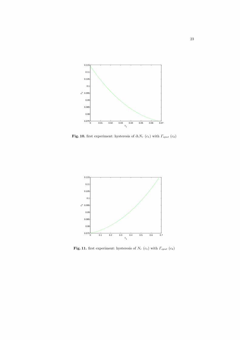
For the solving of the equations we apply the eigenvalue transformation.We present the hysteresises of θtarget with θsubstrate, ∂tNr with Γsput and
Nr with Γsput in the Figures 9, 10 and 11.For solving the coupled equations we apply our algorithm 1.
Second experiment: In our second experiment the variable parameters aregiven with:
Γrsr = 0.05,
Γrγc = 0.02,
Γrγm = 0.1.
We get the following simplified system of ODE’s:
∂tθtarget = −0.07θtarget + 0.1θsubstrate + 0.05, t ∈ (0, T ), (58)
∂tθsubstrate = −0.25
3θsubstrate) +
0.02
3θtarget + 0.05, t ∈ (0, T ), (59)
∂tNr = −0.0125θtarget − 0.0375θsubstrate + 0.05, t ∈ (0, T ), (60)
Γsput = 0.02θtarget) + 0.1θsubstrate, t ∈ (0, T ). (61)
For the solving of the equations we apply the eigenvalue transformation.We present the hysteresises of θtarget with θsubstrate, ∂tNr with Γsput and
Nr with Γsput in the Figures 12, 13 and 14.For solving the coupled equations we apply our algorithm 1.
Third experiment: In our third experiment the variable parameters are givenwith:
Γrsr = 0.05,
Γrγc = 0.1,
Γrγm = 0.02.
We get the following simplified system of ODE’s:
∂tθtarget = −0.15θtarget + 0.02θsubstrate + 0.05, t ∈ (0, T ), (62)

15
∂tθsubstrate = −0.17
3θsubstrate) +
0.1
3θtarget + 0.05, t ∈ (0, T ), (63)
∂tNr = −0.0125θtarget − 0.0375θsubstrate + 0.05, t ∈ (0, T ), (64)
Γsput = 0.1θtarget) + 0.02θsubstrate, t ∈ (0, T ). (65)
For the solving of the equations we apply the eigenvalue transformation.We present the hysteresises of θtarget with θsubstrate, ∂tNr with Γsput and
Nr with Γsput in the Figures 15, 16 and 17.For solving the coupled equations we apply our algorithm 1.
5.3 Sputtering Process with Convection-Diffusion-ReactionEquation
We can describe our model with continuum equations. Since we want to modelthe flow very close to the wafer surface, we assume additionally that the flow isdominated by diffusion.
We have the following equation to simulate a first PVD process or sputteringprocess.
∂tu + v · ∇u = uin(t) in Ω × (0, T ), (66)
u0(x, y) = 0 on Ω,
∂tu(x, y, 0) = u1(x, y) = 0,
u(x, y, t) = 0 on Γ1,
v∂u
∂n= uout on Γ2,
where the constant inflow source is given as uin(t) and we move the source withrespect to the time. So we obtain a sharp step by step processing of differentplasma rays. The bottom boundary Γ2 is the outflow boundary, whereas the restof the boundary Γ1 is a Dirichlet boundary.
We discretize the spatial terms with finite volume methods and apply theBDF method for the time discretization.
Our time steps are given in the Courant number and we apply solver methodsthat are based on different grid levels, e.g. multi-grid methods.
Figure 18, we present the different phases for the flow field in a simplifiedsputter process in 2D. To discuss the deposition rates at the metallic bipolarplate, we present in Figure 18 also the growth rate of the flux model in 2D.
Remark 7. The model can be used to have an overview to vertical gas flows andthe amount of sublimated concentration to the thin film. We can compute thegrowth rate depending on the outflow of the gas concentration. The simulationsare done with Mathematica and numerically with UG.
6 Conclusions and Discussions
We present a continuous model, due to a fare field and near field idea for a flowfield in a PVD apparatus. Based on different models we can predict the flow of

16
the reacting chemicals on the different scales of the chemical reactor. For themesoscopic scale model, we discuss the discretization and solver methods. Wecontribute a coupling algorithm to mix analytical and numerical solutions in ourmodels. Such schemes have benefits in computations and improve the accuracy.Numerical examples are presented to discuss the influence of near-continuumregime at the thin film. The modeling of various inflow sources can describe thegrowth of the thin-film at the wafer. In future, we will analyze the validity ofthe models with physical experiments.
References
1. S. Berg and T. Nyberg. Fundamental understanding and modeling of reactive
sputtering processes. Thin Solid Films, 476, 215-230, 2005.2. P. Bastian, K. Birken, K. Eckstein, K. Johannsen, S. Lang, N. Neuss, and H. Rentz-
Reichert. UG - a flexible software toolbox for solving partial differential equations.Computing and Visualization in Science, 1(1):27–40, 1997.
3. D.J. Christie. Target material pathways model for high power pulsed magnetron
sputtering. J.Vac.Sci. Technology, 23:2, 330-335, 2005.4. I. Farago, and Agnes Havasi. On the convergence and local splitting error of dif-
ferent splitting schemes. Eotvos Lorand University, Budapest, 2004.5. P. Csomos, I. Farago and A. Havasi. Weighted sequential splittings and their anal-
ysis. Comput. Math. Appl., (to appear)6. K.-J. Engel, R. Nagel, One-Parameter Semigroups for Linear Evolution Equations.
Springer, New York, 2000.7. I. Farago. Splitting methods for abstract Cauchy problems. Lect. Notes Comp.Sci.
3401, Springer Verlag, Berlin, 2005, pp. 35-458. I. Farago, J. Geiser. Iterative Operator-Splitting methods for Linear Problems.
Preprint No. 1043 of the Weierstrass Institute for Applied Analysis and Stochastics,Berlin, Germany, June 2005.
9. J. Geiser. Numerical Simulation of a Model for Transport and Reaction of Radionu-
clides. Proceedings of the Large Scale Scientific Computations of Engineering andEnvironmental Problems, Sozopol, Bulgaria, 2001.
10. J. Geiser. Gekoppelte Diskretisierungsverfahren fur Systeme von Konvektions-
Dispersions-Diffusions-Reaktionsgleichungen. Doktor-Arbeit, Universitat Heidel-berg, 2003.
11. J. Geiser. Discretization methods with analytical solutions for convection-diffusion-
dispersion-reaction-equations and applications. Journal of Engineering Mathemat-ics, published online, Oktober 2006.
12. J. Geiser. Discretisation and Solver Methods with Analytical Methods for
Advection-Diffusion-reaction Equations and 2D Applications. Journal of PorousMedia, Begell House Inc., Redding, USA, accepted March, 2008.
13. J. Geiser. Iterative Operator-Splitting Methods with higher order Time-IntegrationMethods and Applications for Parabolic Partial Differential Equations. Journal ofComputational and Applied Mathematics, Elsevier, Amsterdam, The Netherlands,217, 227-242, 2008.
14. J. Geiser. Decomposition Methods for Partial Differential Equations: Theory andApplications in Multiphysics Problems. Habilitation Thesis, Humboldt Universityof Berlin, Germany, under review, July 2008.

17
15. M.K. Gobbert and C.A. Ringhofer. An asymptotic analysis for a model of chemical
vapor deposition on a microstructured surface. SIAM Journal on Applied Mathe-matics, 58, 737–752, 1998.
16. H.H. Lee. Fundamentals of Microelectronics Processing McGraw-Hill, New York,1990.
17. Chr. Lubich. A variational splitting integrator for quantum molecular dynamics.
Report, 2003.18. S. Middleman and A.K. Hochberg. Process Engineering Analysis in Semiconductor
Device Fabrication McGraw-Hill, New York, 1993.19. M. Ohring. Materials Science of Thin Films. Academic Press, San Diego, New
York, Boston, London, Second edition, 2002.20. P.J. Roache. A flux-based modified method of characteristics. Int. J. Numer.
Methods Fluids, 12:12591275, 1992.21. T.K. Senega and R.P. Brinkmann. A multi-component transport model for non-
equilibrium low-temperature low-pressure plasmas. J. Phys. D: Appl.Phys., 39,1606–1618, 2006.
22. J. Stoer and R. Burlisch. Introduction to numerical analysis. Springer verlag, NewYork, 1993.

18
0 2 4 6 8 10−0.2
0
0.2
0.4
0.6
0.8
1
1.2
t
y
Fig. 1. 1D experiment of the heavy particle transport.green: ctot, red: cA, blue: cB , magenta: csurface

19
0 0.1 0.2 0.3 0.4 0.5 0.6 0.7 0.80
0.02
0.04
0.06
0.08
0.1
0.12
0.14
0.16
0.18
0.2
ca
c surf
ace
Fig. 2. hysteresis of the concentrations ca and csurface
0 2 4 6 8 10−0.2
0
0.2
0.4
0.6
0.8
1
1.2
t
y
Fig. 3. 1D experiment of the heavy particle transport.green: utot, red: u1, blue: u2, magenta: usurface, black: ulost

20
−0.05 0 0.05 0.1 0.15 0.2 0.25 0.30
0.02
0.04
0.06
0.08
0.1
0.12
u1
u 3
Fig. 4. hysteresis of the concentrations u1 and u3
0 20 40 60 80 1000
0.1
0.2
0.3
0.4
0.5
0.6
0.7
0.8
0.9
1
t
y
Fig. 5. 1D experiment of the heavy particle transport.green: c1, red: c2

21
0 200 400 600 800 10000
0.1
0.2
0.3
0.4
0.5
0.6
0.7
0.8
0.9
1
t
y
Fig. 6. 1D experiment of the heavy particle transport.green: c1, red: c2
0 2 4 6 8 100
0.1
0.2
0.3
0.4
0.5
0.6
0.7
0.8
0.9
1
t
y
Fig. 7. 1D experiment of the heavy particle transport.green: c1, red: c2

22
0 20 40 60 80 1000
0.5
1
1.5
2
2.5
3
3.5
4
4.5
t
y
Fig. 8. 1D experiment of the heavy particle transport.green: c1, red: c2
0.75 0.8 0.85 0.9 0.95 10.1
0.2
0.3
0.4
0.5
0.6
0.7
0.8
0.9
1
1.1
c1
c 2
Fig. 9. first experiment: hysteresis of θtarget (c1) with θsubstrate (c2)
23
0 0.01 0.02 0.03 0.04 0.05 0.06 0.070.075
0.08
0.085
0.09
0.095
0.1
0.105
0.11
0.115
c1
c 2
Fig. 10. first experiment: hysteresis of ∂tNr (c1) with Γsput (c2)
0 0.1 0.2 0.3 0.4 0.5 0.6 0.70.075
0.08
0.085
0.09
0.095
0.1
0.105
0.11
0.115
c1
c 2
Fig. 11. first experiment: hysteresis of Nr (c1) with Γsput (c2)

24
0.9 1 1.1 1.2 1.3 1.4 1.5 1.6 1.7 1.80.1
0.2
0.3
0.4
0.5
0.6
0.7
0.8
c1
c 2
Fig. 12. second experiment: hysteresis of θtarget (c1) with θsubstrate (c2)
0.05 0.055 0.06 0.065 0.07 0.075 0.08 0.0850.03
0.04
0.05
0.06
0.07
0.08
0.09
0.1
0.11
c1
c 2
Fig. 13. second experiment: hysteresis of ∂tNr (c1) with Γsput (c2)

25
0 1 2 3 4 5 60.03
0.04
0.05
0.06
0.07
0.08
0.09
0.1
0.11
c1
c 2
Fig. 14. second experiment: hysteresis of Nr (c1) with Γsput (c2)
0.4 0.5 0.6 0.7 0.8 0.9 10
0.2
0.4
0.6
0.8
1
1.2
1.4
c1
c 2
Fig. 15. third experiment: hysteresis of θtarget (c1) with θsubstrate (c2)

26
0.05 0.055 0.06 0.065 0.07 0.075 0.08 0.0850.06
0.065
0.07
0.075
0.08
0.085
0.09
0.095
0.1
0.105
c1
c 2
Fig. 16. third experiment: hysteresis of ∂tNr (c1) with Γsput (c2)
0 1 2 3 4 5 60.06
0.065
0.07
0.075
0.08
0.085
0.09
0.095
0.1
0.105
c1
c 2
Fig. 17. third experiment: hysteresis of Nr (c1) with Γsput (c2)

27
time (in sec) : 10 time (in sec) : 100
time (in sec) : 502
0
200000
400000
600000
800000
1e+06
1.2e+06
1.4e+06
1.6e+06
1.8e+06
0 2e+08 4e+08 6e+08 8e+08 1e+09 1.2e+09
first sourcesecondsourcesecondsourcesecondsourcesecondsourcesecondsourcesecondsourcesecondsourcesecondsourcesecondsource
Fig. 18. 2D experiment of the apparatus with a sputtering source at 3 different timelevels (Initial, Start and Flux Positions) and growth of the thin film at the wafer surface

28
7 Appendix
7.1 Matlab-Code for experiment 1
putA = [-1,0,0; 0.95,-0.1,0; 0,0.095,-0.05 ];yo = [1; 0; 0];to = 0.0;tf = 10.0;n = max(size(A));% compute eigenvalues and eigenvectors[wcol, lambdac] = eig(A);wcolinv = inv(wcol);% set up discretized solution gridnpoints = 1000;c0 = 0;dt = (tf-to)/npoints;for i = 1:1:npoints+1tp(i) = (i-1)*dt +to;end% calculate solutionexplambda = zeros(n,n);yp = zeros(n,npoints);cp = zeros(1,npoints);for i = 1:1:npoints+1for j = 1:nexplambda(j,j) = exp(lambdac(j,j)*(tp(i) - to) );endyp(:,i) = wcol*explambda*wcolinv*yo;if(i¿1)cp(1,i) = c0 + (1/2)*dt*0.05*y1 + (1/2)*dt*0.05*yp(1,i) + (1/2)*dt*0.005*y2+ (1/2)*dt*0.005*yp(2,i) + (1/2)*dt*0.05*y3 + (1/2)*dt*0.05*yp(3,i);c0 = cp(1,i);endy1 = yp(1,i);y2 = yp(2,i);y3 = yp(3,i);end%plotfor j = 1:1:4if (j==1)plot (tp,yp(j,:),’g-’), xlabel( ’t’ ), ylabel ( ’y’ )elseif (j==2)plot (tp,yp(j,:),’r-’), xlabel( ’t’ ), ylabel ( ’y’ )elseif (j==3)plot (tp,yp(j,:),’b-’), xlabel( ’t’ ), ylabel ( ’y’ )

29
elseif (j==4)plot (tp,cp(1,:),’m-’), xlabel( ’t’ ), ylabel ( ’y’ )endhold onendhold off
7.2 Matlab-Code for experiment 2
putA = [ -1, 0, 0.05, 0; 0.58, -0.9, 0, 0; 0.42, 0, -1, 0; 0, 0, 0.95, -1 ];yo = [1;0;0;0];to = 0.0;tf = 10.0;n = max(size(A));c0=0;cl0=0;% compute eigenvalues and eigenvectors
wcol,lambdac= eig(A);wcolinv = inv(wcol);% set up discretized solution gridnpoints = 1000;dt = (tf-to)/npoints;for i = 1:1:npoints+1tp(i) = (i-1)*dt +to;end% calculate solutionexplambda = zeros(n,n);yp = zeros(n,npoints);cp = zeros(1,npoints);cl = zeros(1,npoints);for i = 1:1:npoints+1for j = 1:nexplambda(j,j) = exp(lambdac(j,j)*(tp(i) - to) );endyp(:,i) = wcol*explambda*wcolinv*yo;if(i¿1)cp(1,i)=c0 + (1/2)*dt*0.9*u1 + (1/2)*dt*0.9*yp(2,i) + (1/2)*dt*0.4*u3 + (1/2)*dt*0.4*yp(4,i);c0=cp(1,i);cl(1,i)=cl0 + (1/2)*dt*0.6*u3 + (1/2)*dt*0.6*yp(4,i);cl0=cl(1,i);endu1=yp(2,i);u3=yp(4,i);end
30
% plotfor j = 1:1:(n+2)if (j==1)plot (tp,yp(j,:),’g-’), xlabel( ’t’ ), ylabel ( ’y’ )elseif (j==2)plot (tp,yp(j,:),’r-’), xlabel( ’t’ ), ylabel ( ’y’ )elseif (j==3)plot (tp,yp(j,:),’b-’), xlabel( ’t’ ), ylabel ( ’y’ )elseif (j==4)plot (tp,yp(j,:),’y-’), xlabel( ’t’ ), ylabel ( ’y’ )elseif (j==5)plot (tp,cp(1,:),’m-’), xlabel( ’t’ ), ylabel ( ’y’ )elseif (j==6)plot (tp,cl(1,:),’k’), xlabel( ’t’ ), ylabel ( ’y’ )endhold onendhold off
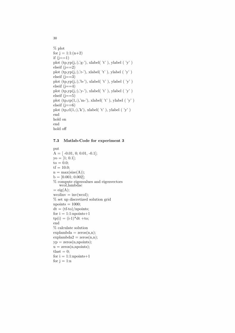
7.3 Matlab-Code for experiment 3
putA = [ -0.01, 0; 0.01, -0.1];yo = [1; 0.1];to = 0.0;tf = 10.0;n = max(size(A));b = [0.001; 0.002];% compute eigenvalues and eigenvectors
wcol,lambdac= eig(A);wcolinv = inv(wcol);% set up discretized solution gridnpoints = 1000;dt = (tf-to)/npoints;for i = 1:1:npoints+1tp(i) = (i-1)*dt +to;end% calculate solutionexplambda = zeros(n,n);explambda2 = zeros(n,n);yp = zeros(n,npoints);u = zeros(n,npoints);tlast = 0;for i = 1:1:npoints+1for j = 1:n

31
explambda(j,j) = exp( lambdac(j,j)*(tp(i) - to) );explambda1(j,j) = exp(-lambdac(j,j)*tlast);explambda2(j,j) = exp(-lambdac(j,j)*tp(i));endif(i greater 1)u(:,i) = u1 + (1/2)*dt*explambda1*wcolinv*b(:,1) + (1/2)*dt*explambda2*wcolinv*b(:,1);yp(:,i) = wcol*explambda*wcolinv*yo + wcol*exp(lambdac(j,j)*tp(i))*u(:,i);endu1 = u(:,i);tlast = tp(i);end% plotfor j = 1:1:nif (j==1)plot (tp,yp(j,:),’g-’), xlabel( ’t’ ), ylabel ( ’y’ )elseif (j==2)plot (tp,yp(j,:),’r-’), xlabel( ’t’ ), ylabel ( ’y’ )endhold onendhold off
7.4 Matlab-Code for experiment 4
putA = [ -0.01, 0; 0.01, -0.1];yo = [1; 0.1];to = 0.0;tf = 10.0;n = max(size(A));b = [0.001; 0.002];% compute eigenvalues and eigenvectors
wcol,lambdac= eig(A);wcolinv = inv(wcol);% set up discretized solution gridnpoints = 1000;dt = (tf-to)/npoints;for i = 1:1:npoints+1tp(i) = (i-1)*dt +to;end% calculate solutionexplambda = zeros(n,n);explambda2 = zeros(n,n);yp = zeros(n,npoints);u = zeros(n,npoints);

32
tlast = 0;for i = 1:1:npoints+1for j = 1:nexplambda(j,j) = exp( lambdac(j,j)*(tp(i) - to) );explambda1(j,j) = exp(-lambdac(j,j)*tlast);explambda2(j,j) = exp(-lambdac(j,j)*tp(i));endif(i greater than 1)u(:,i) = u1 + (1/2)*dt*explambda1*wcolinv*(b(:,1)*(tlast))+ (1/2)*dt*explambda2*wcolinv*(b(:,1)*(tp(i)));yp(:,i) = wcol*explambda*wcolinv*yo + wcol*exp(lambdac(j,j)*tp(i))*u(:,i);endu1 = u(:,i);tlast = tp(i);end%plotfor j = 1:1:nif (j==1)plot (tp,yp(j,:),’g-’), xlabel( ’t’ ), ylabel ( ’y’ )elseif (j==2)plot (tp,yp(j,:),’r-’), xlabel( ’t’ ), ylabel ( ’y’ )endhold onendhold off