Model Reduction for Dynamic Real-TimeOptimization of Chemical Processes

Cover design by Rob Bergervoet

Copyright c©2005 Edoch

Model Reduction for Dynamic Real-TimeOptimization of Chemical Processes

PROEFSCHRIFT

ter verkrijging van de graad van doctoraan de Technische Universiteit Delft,

op gezag van de Rector Magnificus prof.dr.ir. J.T. Fokkema,voorzitter van het College voor Promoties,

in het openbaar te verdedigen

op donderdag 15 december om 13:00 uur

door

Jogchem VAN DEN BERG

werktuigkundig ingenieurgeboren te Enschede

Dit proefschrift is goedgekeurd door de promotor:Prof.ir. O.H. Bosgra

Samenstelling promotiecommissie:

Rector Magnificus voorzitterProf.ir. O.H. Bosgra Technische Universiteit Delft, promotorProf.dr.ir. A.C.P.M. Backx Technische Universiteit EindhovenProf.ir. J. Grievink Technische Universiteit DelftDr.ir. P.J.T. Verheijen Technische Universiteit DelftProf.dr.-Ing. H.A. Preisig Norwegian University of Science and TechnologyProf.dr.-Ing. W. Marquardt RWTH AachenProf.dr.ir. P.A. Wieringa Technische Universiteit Delft

Published by: OPTIMA

OPTIMAP.O. Box 841153009 CC RotterdamThe NetherlandsTelephone: +31-102201149Telefax : +31-104566354E-mail: account@ogc.nl

ISBN 90-8559-152-x

Keywords: chemical processes, model reduction, optimization.

Copyright c©2005 by Jogchem van den Berg

All rights reserved. No part of the material protected by this copyright noticemay be reproduced or utilized in any form or by any means, electronic or me-chanical, including photocopying, recording or by any information storage andretrieval system, without written permission from Jogchem van den Berg.

Printed in The Netherlands.

Voorwoord

Na een memorabele tijd van bijna zeven jaar staat dan uiteindelijk toch hetresultaat van mijn onderzoek zwart op wit. En dat doet goed.

Tijdens mijn afstuderen raakte ik er steeds meer van overtuigd dat het zeerde moeite waard zou zijn om een promotieonderzoek te gaan doen. Na enkelegespreken met Ton Backx en Okko Bosgra over een internationaal project, kwamhet onderwerp modelreductie ter sprake waarvan ik meteen geloofde dat het eenboeiend onderwerp zou zijn.

Ik denk met erg veel plezier terug aan de absurdistische gesprekken afgewis-seld met heftige inhoudelijke neuzel discussies. Meestal begon het serieus maargelukkig was er altijd wel iemand met een verfrissende opmerking, om zo hetbelang van de zaak te relativeren.

Een paar mensen wilde ik graag in het bijzonder bedanken. Ten eerste na-tuurlijk Okko die mij alle vrijheid heeft gegeven om mijn eigen plan te trekkenop basis van onze inhoudelijke altijd interessante discussies. Adrie wil ik graagbedanken voor zijn gepassioneerde uitleg over alles was met chemie te makenheeft en voor de rol van klankbord die hij voor mij vervulde. Mijn kamergenotenRob en Dennis, nestor David, Martijn, Eduard, Branko, Camile, Gideon, Leon,Maria, Martijn, Matthijs en Agnes, Carsten, Debbie, Peter, Piet, Sjoerd en Tonwil ik bedanken voor alle koffietafelgesprekken en borrelpraat. Ook wil ik mijncollega’s van het project bedanken waaronder Martin, Jitendra, Wolfgang Mar-quardt, Mario, Jobert, Wim, Sjoerd, Celeste, Piet-Jan, Pieter, Peter Verheijen,Johan Grievink. Zonder jullie was het project zeker niet geslaagd.

Tenslotte wil ik mijn ouders bedanken voor de onvoorwaardelijke steun dieik altijd van hen gekregen heb. Mijn broer Mattijs en Kirsten voor Lynn voorwie ik nu eindelijk een goede suikeroom kan zijn. Rob voor het ontwerp van deomslag van mijn boekje en mijn andere vrienden de al die tijd verhalen hebbenmoeten aanhoren over de ups en downs die ik tijdens mijn promotietijd hebgehad. Op naar de volgende uitdaging!

Jogchem van den BergRotterdam, oktober 2005

v

Contents

Voorwoord v

1 Introduction and problem formulation 11.1 Introduction . . . . . . . . . . . . . . . . . . . . . . . . . . . . . . 11.2 Problem exploration . . . . . . . . . . . . . . . . . . . . . . . . . 41.3 Literature on nonlinear model reduction . . . . . . . . . . . . . . 171.4 Solution directions . . . . . . . . . . . . . . . . . . . . . . . . . . 251.5 Research questions . . . . . . . . . . . . . . . . . . . . . . . . . . 281.6 Outline of this thesis . . . . . . . . . . . . . . . . . . . . . . . . . 29

2 Model order reduction suitable for large scale nonlinear models 312.1 Model order reduction . . . . . . . . . . . . . . . . . . . . . . . . 312.2 Balanced reduction . . . . . . . . . . . . . . . . . . . . . . . . . . 372.3 Proper orthogonal decomposition . . . . . . . . . . . . . . . . . . 452.4 Balanced reduction revisited . . . . . . . . . . . . . . . . . . . . . 502.5 Evaluation on a process model . . . . . . . . . . . . . . . . . . . 622.6 Discussion . . . . . . . . . . . . . . . . . . . . . . . . . . . . . . . 73

3 Dynamic optimization 753.1 Base case . . . . . . . . . . . . . . . . . . . . . . . . . . . . . . . 753.2 Results . . . . . . . . . . . . . . . . . . . . . . . . . . . . . . . . . 853.3 Model quality . . . . . . . . . . . . . . . . . . . . . . . . . . . . . 863.4 Discussion . . . . . . . . . . . . . . . . . . . . . . . . . . . . . . . 88

4 Physics-based model reduction 894.1 Rigorous model . . . . . . . . . . . . . . . . . . . . . . . . . . . . 894.2 Physics-based reduced model . . . . . . . . . . . . . . . . . . . . 95

vii

4.3 Model quality . . . . . . . . . . . . . . . . . . . . . . . . . . . . . 1014.4 Discussion . . . . . . . . . . . . . . . . . . . . . . . . . . . . . . . 105

5 Model order reduction by projection 1075.1 Introduction . . . . . . . . . . . . . . . . . . . . . . . . . . . . . . 1075.2 Projection of nonlinear models . . . . . . . . . . . . . . . . . . . 1105.3 Results of model reduction by projection . . . . . . . . . . . . . . 1135.4 Discussion . . . . . . . . . . . . . . . . . . . . . . . . . . . . . . . 123

6 Conclusions and future research 1276.1 Conclusions . . . . . . . . . . . . . . . . . . . . . . . . . . . . . . 1276.2 Future research . . . . . . . . . . . . . . . . . . . . . . . . . . . . 130

Bibliography 140

List of symbols 141

A Gramians 143A.1 Balancing transformations . . . . . . . . . . . . . . . . . . . . . . 143A.2 Perturbed empirical Gramians . . . . . . . . . . . . . . . . . . . 145

B Proper orthogonal decomposition 147

C Nonlinear Optimization 149

D Gradient information of projected models 153

Summary 155

Samenvatting 157

Curriculum Vitae 159

viii

Chapter 1

Introduction and problemformulation

This thesis explores possibilities of model reduction techniques for online opti-mization based control in chemical process industry. The success of this controlapproach on industrial scale problems started in petrochemical industry and be-comes now adopted by chemical process industry. This is a challenge becausethe operation of chemical plants differs from petrochemical plant operation im-posing different requirements on optimization based control and consequently onprocess models. For online optimization based control we have limited computa-tional time so computational load is a critical issue. This thesis focusses on themodels and their contribution to online optimization based control.

1.1 Introduction

The value of models in process industries becomes apparent in practiceand literature where numerous successful applications are reported of steady-state plant design optimization and model based control. This developmentwas boosted by maturing commercial modelling tools and continuously increas-ing computing power. Side effect of this development is that not only largerprocesses with more unit operations can be modelled but each unit operationcan be modelled in more detail as well. Especially spatially distributed sys-tems, such as distillation columns and tubular reactors, are well known modelsize boosters.

Large-scale models are in principle not a problem, at the most inconvenientfor the model developer because of the long simulation times involved. Appli-cation of models in an online setting seriously pushes the demands on models

1

to its limits since the available time for computations is limited. Numeroussolutions are thinkable that contribute in solving this issue varying from buyingfaster computers to solving approximate, less computational demanding, controlproblems.

Industry focusses on implementation of effective optimization based controlsolutions whereas university groups focus on understanding of (in)effectivenessof these solutions. Understanding gives direction to development of more ef-fective solutions suitable for industrial applications. This thesis is the resultof close collaboration between industry and universities aiming at symbiosis ofthese two different focusses.

Online optimization

From digital control theory (see e.g. Astrom and Wittenmark, 1997) we knowthat sampling introduces a delay in the control system, limiting controller band-width. The sampling period is therefore preferably chosen as short as possi-ble. A similar situation holds for online optimization. When applying onlineoptimization-based control we can make a tradeoff between a high precisionsolution with a long sampling period and an approximate solution at short sam-pling period. In case of a fairly good model and low frequently disturbances, alow sample rate would most probably be sufficient. However, a tight quality con-straint in combination with a fast response to a disturbance for the same systemwill require a much higher controller bandwidth to maintain performance. So,the tradeoff between solution accuracy and sampling period depends on plant-model mismatch, disturbance characteristics, plant dynamics and presence ofconstraints.

With current modelling packages, processes can be modelled in great detailand model accuracy seems unquestionable. Unfortunately, in reality we alwayshave to deal with uncertain parameters and stochastic disturbances. One canthink of heat exchanger fouling, catalyst decay, uncertain reaction rates anduncertain flow patterns. This motivates the necessity of a feedback mechanismthat deals with disturbances and uncertainties on a suitable sampling interval.

So we can develop large scale models, based on modelling assumptions, thathave some degree of accuracy. Still we need to estimate some key uncertainparameters online (e.g. heat exchanger fouling) from data. Why not choose fora shorter sampling period enabling a higher controller bandwidth by allowingsome model approximation? At some point there must be a break even pointwhere performance of controller based on an accurate model at low sampling rateis as good as based on a less accurate model at high sampling rate. Applicationsof linear model predictive controllers to mildly nonlinear processes illustratethis successful tradeoff between model accuracy and sample frequency. Thisobservation is the main motivation to research and develop nonlinear model

2

approximation techniques for online optimization based control. Aim of thisapproximative model is to improve performance by adding more accuracy tothe predictive part without being overtaken by the downside of a slightly longersampling period.

Model reduction

Model reduction is not a purpose in itself. Without being specific what is aimedat by reduction, model reduction is meaningless. In this thesis we will assessthe value of model reduction techniques for dynamic real-time optimization.

In system theory we associate model reduction with model-order reduction,which implies a reduction of the number of differential equations. Because li-near model reduction was successful, this notion was carried over to reduction ofprocess models governed by nonlinear differential and algebraic equations (dae).First difference between these two models types is obviously that dae processmodels are nonlinear in their differential part. This nonlinearity was preciselythe extension we looked for since this should improve model accuracy. Seconddifference is that dae process models consist of many algebraic equations. Incase of a set of (index one) nonlinear differential algebraic equations in generalwe cannot eliminate these algebraic equations by analytical substitution, bring-ing us back to ordinary differential equations. This implies we deal with a trulydifferent model structure if implicit algebraic equations are present. This dif-ference has far reaching consequences for the notion of reduction of nonlinearmodels as will become clear later in this thesis.

As discussed in the previous section, both solution accuracy and computa-tional load of the online optimization determine the online performance. In caseof online optimization based control, in principle we do not care about the exactnumber of differential or algebraic variables of a model; model reduction shouldresult in a reduction of the optimization time accepting some small degradationof solution accuracy. Model approximation is an alternative description for themodel reduction that will be used in this thesis since it is less associated tomodel order reduction only.

A model is not only characterized by its number of differential and algebraicequations, but also by structural properties such as sparsity and controllability-observability. Time scales, nonlinearity and steady-state gains are importantproperties as well. The relation between model properties and computationalload and accuracy is not always trivial, which can result in unexpected findingswhen evaluating model reduction techniques. Note further that the model isnot the only degree of freedom within the optimization framework. The suc-cess of model reduction for online optimization-based control depends on theoptimization strategy and implementation details such as choices of solvers andsolver options.

3

Realizing that the final judgement of the success of a model reduction techniquefor online optimization depends on many different choices of implementation weelaborate in the next section on different aspects that effect the optimizationproblem.

1.2 Problem exploration

In this section we will explore different aspects to be considered whendiscussing dynamic real time optimization of large scale nonlinear chemicalprocesses. First of all we need a model representing the process behavior. Thisis not a trivial task but is nowadays supported by various commercially availa-ble tools. Such a model is then confronted with plant data to assess its modelvalidity, which in general requires changes in the model. After several itera-tions we end up with a validated model, which is ready for use within onlineoptimization. Since we are interested in future dynamic evolution of some keyoutput process variables we require simulation techniques to relate them to fu-ture process input variables by simulation. Computation of the best futureinputs is done by formulating and solving an optimization problem. We willtouch on differences between the two main implementation variants to solvesuch a dynamic optimization problem. Finally we will motivate the need formodel reduction by showing the computational consequences of straightforwardimplementation of this optimization problem for the model size that is commonfor industrial chemical processes.

Mathematical models

Numerous different names are available for models, each referring to a specificproperty of the model. One could distinct between models based on conserva-tion laws and data driven models. The first class of models is referred to as firstprinciples, fundamental, rigorous or theoretical models and are in general non-linear dynamic continuous time models. These models are formulated by a setof ordinary differential equations (ode model) or a set of differential algebraicequations (dae model).

The second class of models is referred to as identified, step response orimpulse response models and are in general defined as linear discrete time input-output regressive models. Nonlinear static models can be added to these lineardynamic models giving an overall nonlinear behavior. The subdivision is not asblack and white as stated here and combinations of both classes are possible asthe term hybrid models already implies.

Process models that are used for dynamic optimization in general are for-mulated as a set of differential algebraic equations. In the special case that

4

all algebraic equations can be eliminated by substitution, the dae model canbe rewritten as a set of ordinary differential equations. Distinction betweenthese two models is important because of their different numerical integrationproperties, which will be treated later in this chapter. Characteristic for modelsin process industry are physical property relations that generally do not allowfor elimination by substitution and to a large extent contribute to the numberof algebraic equations. Physical property calculations can also be hidden inan external module interfaced to the simulation software. Caution is requiredinterfacing both pieces of software1.

Partial differential equations (pde model) describe microscopic conservationlaws and emerge naturally in case spatial distributions are modelled. Classicalexamples are the tubular heat exchanger and tubular reactor. Although thistype of models is explicitly mentioned here, the model can be translated into adae-model that approximates the true partial differential equations.

Dae and ode models both have internal variables, which implies that theeffect of all past inputs to the future can be captured by a single value for allvariables of the model at time zero, as opposed to most identified models thatin general are regressive and require historical data to capture future behaviorof past inputs. Disadvantage of continuous time nonlinear models is the com-putational effort for simulation whereas simulation with a discrete time modelis trivial. On the other hand stability of a nonlinear discrete time model isnontrivial. Advantage of rigorous models is that they in general have a largervalidity range than identified models because of their fundamental origin of non-linear equations. Nonlinear identification techniques of dynamic processes areemerging but are still far from mature.

Although modelling still can be tedious, developments by commercial processsimulation and modelling tools such as gPROMS� and Aspen CustomModeler�

allow people with different modelling skills to use and build rigorous modelsquite efficiently. A graphical user interface with drag and drop features in-creased the accessability for more people than only diehard command promptprogrammers. Still, thorough modelling knowledge is required to deal with fun-damental problems such as index problems.

All mathematical models can be described by its structure and parameters.Fundamental question is how to decide on model structure and how to inter-pret mismatch between plant and simulated data. Do we need to change modelstructure or do we need to change model parameter values? No tools are availa-ble how to discriminate between those two options not to mention help findinga better structure.

1Error handling in the external module can conflict with error handling by the simulationsoftware.

5

In case we do have a match between plant and simulated data, we could have thesituation where not all parameters can be uniquely determined from availableplant data. Danger is that the match for this specific data can be satisfactory butusing a new data set could give a terrible match. Whenever possible it seemswise to arrange parameters in order of uncertainty. Dedicated experimentscan decrease uncertainty of specific parameters such as activity coefficients andpre-exponential factors in an Arrhenius equation or physical properties such asspecific heat. Besides parameter uncertainty we have structural uncertainty dueto lumping based on uncertain flow patterns or uncertain reaction schemes. Insome cases we can interchange model uncertainty by parameter uncertainty byadding a structure that can be inactivated by a parameter. Risk is that we endup with too many parameters to be determined uniquely from available data.Computation of the values of model parameters will be discussed in the nextsection.

Identification and validation

Computation of parameter values can be formulated as a parameter optimizationproblem and is referred to as a parameter estimation problem in case the modelstructure is based on first principles. In case model structure is motivatedby mathematical arguments, identification is more commonly used to addressthe procedure. Basically both boil down to a parameter optimization problemminimizing some error function.

Important for model validation are the model requirements. Typically,model requirements are defined in terms of error tolerance on key process varia-bles over some predefined operating region. Most often these are steady-stateoperating points but these requirements can also be checked for dynamic ope-ration. Less common is a model requirement defined in terms of a maximumcommotional effort. The objective of a parameter identification is to find thoseparameters that minimizes the error over this operation region.

Resulting parameter values of either estimation or identification are nowready for validation. During the validation procedure parameter values arefixed and the model is used to generate predictions based on new input-outputdata. This split of data is also referred to as estimation data set and validationdata set. From a more philosophical point of view a one could better refer tomodel validation by model unfalsification (Kosut, 1995); a model is valid untilproven otherwise. This touches on the problem that for nonlinear models notall possible input signals can be validated against plant data. For linear modelswe can assess model error because of the superposition principle and dualitybetween time and frequency domain.

Model identification is a data driven approach to develop models. The there-fore required data can either be obtained during normal operation, or as in most

6

cases, from dedicated experiments (e.g. step response tests). Elegant propertyof this approach is that the identified model is both observable and controllable,which is typically not the case for rigorous models. Since only a very limitednumber of modes are controllable and observable this results in low order models.In that sense rigorous modelling can learn from model identification techniques.

Linear model identification is a mature area whereas for nonlinear identi-fication several techniques are available (e.g. Volterra series, neural nets andsplines) without a thorough theoretical foundation. Neural networks have a veryflexible mathematical structure with many parameters. By means of a parame-ter optimization, referred to as training of the neural net, an error criterion isminimized. The result is tested (validated) against data that was not used fortraining.

Many papers are written on this appealing topic with the main focus on para-meter optimization strategy and internal approximative functions and structure.Danger of neural nets is over-fitting, which results in poor interpolative predic-tions. Over-fitting implies that the data used for training is not rich enoughto uniquely determine all parameters (comparable to an under-determined orill-conditioned least squares solution). Extrapolative predictive capability is ac-knowledged to be very bad (Can et al., 1998) and one is even advised to trainthe neural net with data that encloses a little bit more than the relevant ope-rating envelope. This reveals another weak spot of this type of data drivenmodels since data is required at operating conditions that are undesired. Lotsof data is required, which can be very costly if these data has to be generated bydedicated tests. A validated rigorous model can take away part of this problemwhen used as an alternative data generator.

Simulation

Simulation of linear and discrete time models is a straightforward task whereassimulation of continuous time nonlinear models is more involved. In generalsimulation is executed by a numerical integration routine available in manydifferent variants. Basic variants are described in textbooks such as by Shampine(1994), Dormand (1996) and Brenan et al. (1996). The main problem with thismethod is that the efficiency of these routines are strongly effected by heuristicsin e.g. error, step-size and prediction order control, which is less easy to seethrough.

Easily understandable are fixed step-size explicit integration routines likeEuler and Runga-Kutta schemes. The main problem here is the poor efficiencyfor stiff systems due to small integration step-size. The stability region of ex-plicit integration schemes limits step size whereas stability of implicit integrationroutines does not depend on step-size. Implicit fixed step-size integration rou-tines can be viewed as an optimization solved by iterative Newton steps. A well

7

known property of this Newton step based optimization is its fast convergence,given a good initial guesses. Numerous different approaches based on differentinterpolation polynomials are available for this initial guess under which theGear predictor (Dormand, 1996) is probably known best.

Routines with a variable step-size are more tedious to understand, caused byheuristics in step-size control. This control balances step-size with the numberof Newton steps needed for convergence with the objective to minimize compu-tational load. Similarly the order of the prediction mechanism may be variableand controlled by heuristics. Inspection of all options reveals that many han-dles are available to influence the numerical integration (e.g. absolute tolerance,relative tolerance, convergence tolerance, maximum iterations, maximum itera-tion of no improvement, effective zero, perturbation factor, pivot search depth,etc.). Fixed step-size numerical integration routines exhibit a variable numericalintegration error with a pre-computed upper bound whereas variable step-sizeroutines maximize step-size constraint to a maximum integration error tole-rance.

Experience learns that consistent initialization of dae models is a delicateissue and far from trivial, since it reduces to an optimization problem withas many degrees of freedom as variables that are to be initialized (easily overtens of thousands of variables). Not only does a good initial guess speed upconvergence, in practice it appears to be a necessity; with a default initial guess,initialization will most probably fail. Modelling of dae systems in practice isdone by developing a small model that gradually is extended, reusing previouslyconverged initial values as an (incomplete) initial best guess of both algebraicand differential variables.

Numerical integration routines were developed for autonomous systems. Dis-continuities can be handled but at cost of a (computationally expensive) re-initialization. Since a digital controller would introduce a discontinuity at everysample time, and consequently require a re-initialization, it can be attractiveto approximate this digital controller by its analogue (continuous) equivalentif possible. For simulation of optimal trajectories defined on a basis of discon-tinuous functions, it might be worthwhile to approximate the trajectory by aset of continuous and differentiable basis-functions. This reduces the number ofre-initializations and therefore can improve computational efficiency, unless thestep-size has to be reduced drastically where the differentiable approximationintroduces large gradients.

Selecting a solver and fine tuning solver options balancing speed and robust-ness is a tedious exercise and makes it hard to derive general conclusions aboutdifferent available solvers. Generally models of chemical processes exhibit diffe-rent time-scales (stiff system) and a low degree of interacting variables (sparsity).Sparse implicit solvers deal with this type of models very efficiently.

8

Optimization

Like in the world of modelling, the field of dynamic optimization has its ownjargon to address specific characteristics of the problem. Most optimizationproblems in process industry can be characterized as non-convex, nonlinear,constrained optimization problems. In practice this implies that only local op-timal solutions can be found instead of global optimal solutions.

The presence of constraints requires constraint handling, which can be donein different ways (see e.g. textbooks by Nash and Sofer, 1996 and Edgar andHimmelblau, 1989). Often these constraints are multiplied with Lagrange mul-tipliers and added to the objective, which transforms the original optimizationproblem into an unconstraint optimization problem. We can distinguish be-tween penalty and barrier functions. The penalty function approach allows for(intermediate) solutions that violate constraints (most probably they will, sincesolutions tend to be at the constraint), whereas the barrier function approachrequires a feasible initial guess and from this solution guarantees feasibility.Finding a feasible initial guess can already be very challenging, which explainsthe popularity of the penalty function approach.

For steady-state plant (Floudas, 1995) design optimization, typical optimiza-tion parameters are equipment size, recycle flows and operating conditions liketemperature, pressure and concentration. Discrete decision variables to deter-mine the type of equipment (or number of distillation trays) yield a computa-tional hard optimization known as a mixed integer nonlinear program (minlp).

The optimization problem to be solved for computation of optimal input tra-jectories is referred to as a dynamic optimization problem and generally assumessmooth nonlinear models without discontinuities. Using a parametrization ofthese trajectories by means of basis functions and coefficients, such a problemcan be written as a nonlinear program. The choice of basis functions determinesthe set of possible solutions. A typical set of basis functions consists of functionsthat are one for a specific time interval and zero otherwise. This basis allows aprogressive distribution of decision variables over time, which is very commonlyused in online applications. A progressive basis reflects the desire (or expecta-tion!) to have an optimal solution with (possible) high frequent control movesin the beginning and low frequent control moves towards the end of the controlhorizon. Since a clever choice of basis functions could reduce the number ofbasis functions (and consequently the number of parameters for optimization)this is an interesting field of research.

For the solution of dynamic optimization problems we need to distinguish be-tween the sequential and simultaneous approach (Kraft, 1985; Vassilidis, 1993).The sequential approach computes a function evaluation by simulation of themodel followed by a gradient based update of the solution. This sequence is re-

9

peated until solution tolerances are satisfied (converged solution) or some othertermination criterion is satisfied (non converged solution).

In the simultaneous approach, also referred to as collocation method (Neu-man and Sen, 1973; Biegler, 2002), not only the input trajectory is parame-terized but the state trajectories as well. This trajectory is described by a setof basis functions and coefficients from which the time derivatives can be com-puted. At each discrete point in time this trajectory time derivative shouldsatisfy the time derivative defined by the model equations. This results in anonlinear program (nlp) type of optimization problem were the objective isminimized subjected to a very large set of coupled equality constraints repre-senting the process behavior. The free parameters of this nlp are both theparameters that define the input trajectory and parameters that describe thestate trajectory. Since mathematically there is no difference between these para-meters and all parameters are updated each iteration step together, this methodis called the simultaneous approach.

In general the sequential approach outperforms the simultaneous approachfor large systems. This is not a rigid conclusion since in both areas researchersare developing better algorithms exploiting structure and computationally cheapapproximations. Note that in case of the sequential approach during all (inter-mediate) solutions the model equations are satisfied by means of simulation.In case of the simultaneous approach intermediate solutions generally do notsatisfy model equations. Note furthermore that with a fixed input trajectorythe collocation method is an alternative for numerical integration.

Both the sequential as well as the simultaneous approach are implemented asan approximate Newton step type of optimization. The Hessian is approximatedby an iterative scheme efficiently reusing derivative information. A true Newtonstep is simply not worthwhile because of its computational load. Optimizationroutines require a sensitivity function of optimization parameters with respectto the objective function (and constraints). This sensitivity function is reflectedby partial derivatives that can be computed by numerical perturbation or inspecial cased by analytical derivatives.

Jacobian information generated during simulation can be used to build alinear time variant model along the trajectory, which proves to be an efficientand suitable approximation of the partial derivatives. Furthermore, parame-tric sensitivity can also be derived by integration of sensitivity equations or bysolving adjoint equations. Reuse of Jacobian information from the simulationand exploitation of structure can reduce the computational load resulting in anattractive alternative.

10

Industrial process operation and control

Process operation covers a very wide area and involves different people through-out the company. The main objective the plant operation is to maximize profi-tability of the plant.

Primary task of plant operation is safeguarding. Safety of people and envi-ronment always gets highest priority. In order to achieve this, hardware mea-sures are implemented. Furthermore, measurements are combined to determinethe status of the plant. If a dangerous situation is detected, a prescribed sce-nario is launched that shuts down the plant safely. For the detection as wellas for the development of scenarios, models can be employed. Fault detectioncan be considered as a subtask within the safeguarding system. It involves thedetermination of the status of the plant. A fault does not always induce a plantshutdown but can also trigger a maintenance action.

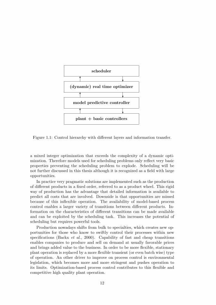
Basic control is the first level in the hierarchy as depicted in Figure 1.1providing control actions to keep the process at desired conditions. Unstableprocesses can be stabilized allowing safe operation. Typically, basic controllersreceive temperature, pressure and flow measurements and act on valve positions.Furthermore, all kinds of smart control solutions are developed to increase per-formance. Different linearizing transformation schemes and decoupling ratio andfeed forward schemes are implemented in the distributed control system (dcs)and perform quite well. These schemes are to a high degree based on processknowledge, but nevertheless not referred to as advanced process control.

Steady-state energy optimization (pinch) studies can reduce energy costs byrearranging energy streams (heat integration). Side effect is the introductionof (undesired) interaction of different parts of a plant. An upset downstreamcan act as a disturbance upstream without a material recycle present. Materialrecycle streams are known to introduce large time constants of several hours(Luyben et al., 1999). Both heat integration and material recycles complicatecontrol for operators.

Automation of the process industry took place very gradually. Nowadaysmost measurements are digitally available in the control room from which prac-tically all controls can be executed. The availability of these measurements werea necessity for the development of advanced process control techniques, such asmodel predictive control (see tutorial paper by Rawlings, 2000), and because ofits success, it initiated real-time process optimization.

Scheduling can be considered as the top level of plant operations (Tousain,2002) as depicted in Figure 1.1. At this level it is decided what product isproduced at what time and sometimes even by which plant. Processing of in-formation from the sales and marketing department, the purchase department,storage of raw material and end products is a very complex task. Withoutradical simplifications, implementation of a scheduling problem would result in

11

scheduler

(dynamic) real time optimizer

✻ ❄

model predictive controller

✻ ❄

plant + basic controllers

✻ ❄

Figure 1.1: Control hierarchy with different layers and information transfer.

a mixed integer optimization that exceeds the complexity of a dynamic opti-mization. Therefore models used for scheduling problems only reflect very basicproperties preventing the scheduling problem to explode. Scheduling will benot further discussed in this thesis although it is recognized as a field with largeopportunities.

In practice very pragmatic solutions are implemented such as the productionof different products in a fixed order, referred to as a product wheel. This rigidway of production has the advantage that detailed information is available topredict all costs that are involved. Downside is that opportunities are missedbecause of this inflexible operation. The availability of model-based processcontrol enables a larger variety of transitions between different products. In-formation on the characteristics of different transitions can be made availableand can be exploited by the scheduling task. This increases the potential ofscheduling but requires powerful tools.

Production nowadays shifts from bulk to specialties, which creates new op-portunities for those who know to swiftly control their processes within newspecifications (Backx et al., 2000). Capability of fast and cheap transitionsenables companies to produce and sell on demand at usually favorable pricesand brings added value to the business. In order to be more flexible, stationaryplant operation is replaced by a more flexible transient (or even batch wise) typeof operation. An other driver to improve on process control is environmentallegislation, which becomes more and more stringent and pushes operation toits limits. Optimization-based process control contributes to this flexible andcompetitive high quality plant operation.

12

Economic dynamic real time optimization plays a key role in bringing moneyto the business, since it translates a schedule into economically optimal setpoint trajectories for the plant. At least as important is the feedback that thedynamic optimization can give to the scheduling optimization in terms of e.g.minimal required transition times and estimated costs of different and possiblenew transitions. This information, depicted by the arrow from dynamic realtime optimization to the scheduler in Figure 1.1, enables improved schedulingperformance because the information is more accurate and complete and allowsfor more flexible operation. This more enhanced information can, for example,bring the difference between accepting and refusing a customers order. Dynamicreal-time optimization plays a crucial role in connecting scheduling to plantcontrol and can give a significant contribution to the profitability of a plant.

Real-time process optimization

state of the art operated plants have a layered control structure where theplants steady-state optimum is computed recursively by the real-time processoptimizer providing set points that are tracked by a linear model predictivecontroller. Besides that this approach was implementable from a computationalpoint of view, from the operators perspective, this approach was acceptable todo as well, with a safety argument that pleads for a layered control structure.In case of failure of the real-time optimization the process is not out of controlbut only the optimization is not executed.

Since a state of the art optimizer assumes some steady-state condition, thiscondition is checked before the optimizer is started (Backx et al., 2000). Thischeck is somewhat arbitrary because in practice a plant is never in steady state.Before the next steady-state optimization is executed a parameter estimationis carried out using online data. The result of the steady-state optimization isa new set of set points causing a dynamic response of the plant. Only afterthe process is stable again a next cycle can be started, which limits the updatefrequency of optimal set points. If a process is operated quasi steady-state andoptimal conditions change gradually this approach can be very effective.

For a continuous process that produces different products we require eco-nomical optimal transitions from one operation point to the other. Includingprocess dynamics in the optimization enables exploitation of the full potentialof the plant. Result of this optimization approach will be a set of optimal setpoint trajectories and a predicted dynamic response of the process. In this ap-proach we do not require steady-state conditions to start an optimization andit enables shorter transition times. Shorter transition times generally result inreduction of off spec material and therefore increase profitability of a plant.

The real-time, steady-state optimizer and linear model predictive controllercan be replaced by a single dynamic real-time optimization (drto) based on one

13

.................................................................................................

.................................................................................................✲

✛

✲❄

✲❄✲❄

......................................

.....................

......................................

.....................

......................................

.....................

......................................

.....................

......................................

.....................✲

✛ ✲❄

❄

✛

......................................

..................... ...........................................................

......................................

.....................

......................................

..................... ...........................................................

...........................................................

...........................................................

....................................................

....................................................

✠❄

✲

✒........................................................... ......................................

.....................

......................................

.....................

......................................

..................... ...........................................................

...........................................................

...........................................................

....................................................

....................................................

✠❄

✲

✲✛

✲

✒........................................................... ......................................

.....................

......................................

.....................

......................................

..................... ...........................................................

...........................................................

...........................................................

....................................................

....................................................

✠❄

✲

✲

✲

✲

✒

Figure 1.2: Typical chemical process flow sheet with multiple different unitoperations and material recycle streams representing behavior of a broad classof industrial processes.

large-scale nonlinear dynamic process model. This problem should be solvedat the sample rate of the model predictive controller to maintain similar dis-turbance rejection properties as the linear model predictive controller. Theprediction horizon of the optimization should be a couple of times the processdominant time constant. The implication of this straightforward implementa-tion is discussed next.

Implications straightforward implementation

Let us now explore what the implication is of straightforward implementationof dynamic real-time optimization as a replacement of the real-time steady-state optimizer and linear model predictive controller. In a typical chemicalprocess, two or more components react into the product of interest followedby one or more separation steps. This represents typical behavior of a broadclass of industrial processes and therefore findings can be carried over to manyplants. In general, one or more side reactions take place introducing extracomponents. The use of a catalyst can shift selectivity but never prevent sidereactions completely. Suppose we assume only one side reaction, we alreadyhave to deal with four species, or even five if we take the catalyst into account.We can separate the four species with three distillation columns as depicted inFigure 1.2 if we assume that the catalyst can be separated by a decanter. Therecycle streams introduce positive feedback and therefore long time constantsin the overall plant dynamics (Luyben et al., 1999).

Suppose we assume a instantaneous phase equilibrium and uniform mixingon each tray, the number of differential equation that describes the separation

14

of this chemical process is

nx = nc(ns + 1)(nt + 2) ,

where nx is the number of differential equations, nc is the number of columns,ns is the number of species that are involved and nt is the average number oftrays per column. The one in the formula represent the energy balance and thetwo represents the reboiler and condensor of a column. For a setup with threecolumns with twenty, forty and sixty trays and five species we need already overseven hundred and fifty differential equations. If the reaction takes place ina tubular reactor we need to add a partial differential equation to the model.This can only be implemented after discretization, easily adding another treehundred equations (five species times sixty discretization points) to the modelbringing the total over a thousand equations. So we can extend the previousformula to

nx = nc(ns + 1)(nt + 2) + nsnd ,

where nd is the number of discretization points. In practice the number ofalgebraic variables is three to ten times the number of differential equations,depending on implementation of physical properties (as hidden module or asexplicit equations in the model). This brings the total of equations to seve-ral thousands up to ten thousand equations. This estimate serves as a lowerbound for a first principle industrial process model, and illustrates the number ofequations that should be handled by plant-wide model-based process operationtechniques.

Fortunately the models are very nicely structured that can be exploited. Thismodel property is referred to as the model sparsity and reflects the interactionor coupling between equations and variables. This property can be visualized bya matrix, the so-called Jacobian matrix J . If the jth variable occurs in the ith

equation the J(i, j) element is nonzero and zero otherwise. Most zero elementsare structural so do not depend on variable values. These elements do not haveto be recomputed during simulation, which allows for efficient implementationof simulation algorithms. The number of nonzero elements for process modelsis about five to ten percent of the total elements of the Jacobian matrix.

Next we will estimate the number of manipulated variables that are involved.Every column has five manipulated variables: the outgoing flows from reboilerand condensor, reboiler duty, condenser duty and the reflux rate or ratio. Inthis simple example we can manipulate within the reactor the fresh feed flowand composition, feed to catalyst ratio, cooling rate and outgoing flow of thereactor. This brings the number of manipulated variables to twenty, all poten-tial candidates to be computed by model-based optimization. The number of

15

parameters that is involved can be computed by the next formula:

np =nuH

ts,

where np is the number of free parameters, nu is the number of manipulatedvariables, H is the control horizon and ts is the sampling rate. For a typicalprocess as described in this section, the dominant time constant can be overa day, especially if recycle streams are present introducing positive feedback.An acceptable sampling rate for most manipulated variables is a sampling rateof one to five minutes, however, pressure control might require a much highersampling rate. In case of a horizon of three times the dominant time constant,twenty inputs and a sampling rate of five minutes, the total number of free pa-rameters is over seventeen thousand. This results in a very large optimizationproblem that is not very likely to give sensible results. A selection of manipu-lated variables and clever parametrization of the input signals can reduce thisnumber of free parameters. The input signal can even be implemented as afully adaptive, problem-dependent parameterization generated by repetitive so-lution of increasingly refined optimization problems (Schlegel et al., 2005). Theadaptation is based on a wavelet analysis of the solution profiles obtained in theprevious step.

In practice, first some base layer control would be implemented around eachcolumn to control levels and pressures. Set points for these controllers couldthen be degree of freedom for optimization. The added value of including theseset points within a dynamic optimization are not evident but small inventoriescould decrease transition times. If for some reason the added value of thesedegrees of freedom are expected to be small they can be removed from theoptimization problem reducing the number of optimization parameters.

Suppose we want to do one nonlinear integration of the rigorous model withinone sampling period to do a prediction of an input trajectory. In this casewe need to simulate three days within five minutes. This requires at leastsimulation speed of over eight hundred times real time. If a sampling period ofone hour is acceptable we still need a simulation speed of seventy two times realtime. In this scenario we did not account for multiple, in case of the sequentialoptimization approach approximately between five and twenty, simulations andother computations than simulation. Depending on the input sequence, forthe size of the models that is considered on current standard computer thesimulation speed is between one to twenty times realtime. This reveals thetremendous gap between desired and current status of numerical integration.Nevertheless, numerical solvers are already very sophisticated handling differenttimescales, also referred to as stiff systems, and exploiting model structure.

With current commercial modelling tools we usually end up with a set ofdifferential and algebraic equations. Keeping the model in line with the process,

16

measurements are used to estimate the actual state of the process by means ofan observer, e.g. an extended Kalman filter (e.g. Lewis, 1986). This is a modelbased filtering technique, balancing model error with measurement error. Theresulting state is then used as a corrected initial condition for the model. Find-ing a consistent solution for this new initial condition for a set of differentialalgebraic equations is called an initialization problem, which is hard to solvewithout a good initial guess. Fortunately, we can use the uncorrected state asinitial guess which should be good enough. Still this initialization problem hasto be solved every iteration at cost of valuable computing time.

Going online with a straightforward implementation of real time dynamic plantoptimization based on first principle models introduces an enormous compu-tational overload. At present only very pragmatic solutions are available thatdirectly provoke all kinds of comments such as the inconsistency that is intro-duced by the use of different models in different layers within the plant operationhierarchy. These approaches are legitimated by the argument that there are nobetter alternatives readily available. Despite all this criticism on the pragmaticsolutions for the model based plant operation, the approach has proven to con-tribute towards the profitability of the plant. This profitability can only beincreased if consistent solutions are developed that replace the pragmatic so-lutions. Model reduction can provide a consistent solution and is explored inthis thesis. First we will continue with model reduction techniques available inliterature.

1.3 Literature on nonlinear model reduction

Models that are available for large scale industrial processes can ingeneral be characterized as a set of differential and algebraic equations (dae).Therefore we search for model reduction techniques that are applicable to thisgeneral class of models. This class of models is capable to describe the majorityof processes and is more general than a set of ordinary differential equations(ode). Transformation of a dae into an ode is not possible in general and isregarded as major model reduction step.

Since we are interested in the effect of different models on computationalload for optimization every technique mapping one model to an other model isa candidate model reduction technique. This implies that different modellingand identification techniques can be considered using the original model as datagenerating plant replacement.Marquardt (2001) states that the proper way to assess model reduction tech-niques for online nonlinear model based control is to compare the closed loopperformance based on the original model, with low sampling frequency, with

17

the reduced model at higher sampling frequency. Maximum sampling frequen-cies are determined by the computational load that is related to the differencesbetween original and reduced model. The reduced model should enable highersampling frequencies compensating for loss in accuracy and therefore result inhigher closed loop performance. None of this type of assessments have beenfound in literature. Therefore we will need to resort to more general literatureon model reduction and nonlinear modelling techniques.

Computation and performance assessment of NLMPC

Findeisen et al. (2002) assessed computation and performance of nonlinearmodel predictive control. The implementation of the control problem used inthis paper was the so-called direct shooting, which is a special efficient imple-mentation of the simultaneous approach (Diehl et al., 2002). In their assessment,different models are compared under closed loop control. The different modelsof the 20 tray distillation column were a nonlinear wave model with 2 differentialand 3 algebraic equations, a concentration and holdup model with 42 ordinarydifferential equations and a more detailed model (including tray temperatures)with 44 differential and 122 algebraic equations. All different models wherethe result of remodelling, thus extra simplifications and assumptions based onphysics and process knowledge resulted in reduced models.

The effect on the computational load is presented even for different con-trol horizons, distinguishing between the maximum and average computationtime. More simplified models resulted in lower computational load, which isnot surprising. More interesting is that the reduction in computational loadis quantified. The increase of controller performance due to higher samplingfrequency enabled by reduced computational effort was not presented. Neitheris completely clear how big the modelling error between original and reducedmodels is.

Load of state estimation for these different reduced models was assessed aswell. Furthermore computational load of different nonlinear predictive schemeswere assessed with the original model in case of no plant model mismatch.

Nonlinear wave approximation

Balasubramhanya and Doyle III (2000) developed a reduced-order model of abatch reactive distillation column using travelling waves. The reader is referredto e.g. Marquardt (1990) and Kienle (2000) for more details on travelling waves.This nonlinear model was successfully deployed within a nonlinear model pre-dictive controller (nlmpc) and linear Kalman filter that was computationallymore efficient than a nlmpc based on the original full-order nonlinear model.Although the original full order model was only a 31st order ode and the re-

18

duced model a 5th order ode, the closed loop performance was over six timesfaster in closed-loop with nlmpc based on the reduced model while maintainingperformance. Performance was quite high despite of prediction horizon of onlytwo samples and a control horizon of one. Furthermore they compared the non-linear models with the linearized model illustrating the level of nonlinearity ofthe process.

Simplified physical property models

Successful use of simplified physical property models within flow sheet optimiza-tion is reported by Ganesh and Biegler (1987). A simple flash with recycle aswell as a more involved ethylbenzene process with reactor, flash, two columnsand two recycle streams are presented in that paper. In both cases the rigo-rous phase equilibrium model (Soave-Redlich-Kwong) was approximated by asimplified model (Raoult’s law, Antoine’s equation and ideal enthalpy). Thistype of model simplification is based on process knowledge and physical insight.It is a tailored approach but applicable to all models where phase equilibriaare to be computed. Reductions up to an order of magnitude were reportedby straightforward use of the simplified model within optimization. Dangerof this approach was already reported by Biegler (1985) and is that the opti-mum does not coincide with the optimum of the original model. Combiningthe rigorous and simplified model in their optimization strategy Ganesh andBiegler can guarantee convergence to the true optimum with the original modeland still reducing the computational load by over thirty percent. Model sim-plification based on physics appears to be successful for steady-state flowsheetoptimization.

Chimowitz and Lee (1985) reported increase of computational efficiency ofa factor of order three by the use of local thermodynamic models. Accordingto Chimowitz up to 90% of computational time was used for thermodynamiccomputations during simulation, motivating their approach of model approxi-mation. The local thermodynamic models are integrated with the numericalsolver where an updating mechanism of the parameters of the local models wasincluded. This approach is not easy to use since model reduction and numeri-cal algorithm are integrated. Ledent and Heyen (1994) attempted to use localmodels within dynamic simulations but were not successful due discontinuitiesintroduced by updating the local models. Still local models as such, without up-date mechanism, can be used reducing computational load despite their limitedvalidity.

Perregaard (1993) worked on model simplification and reduction for simu-lation and optimization of chemical processes. The objective of his paper is topresent a simplification procedure of the algebraic equations that through simpli-fication of the algebraic equations for phase equilibria calculations is capable of

19

reducing the computing time to solve the model equations without effecting theconvergence characteristics of the numerical method. Furthermore it exploitsthe inherited structure of equations representing the chemical process. Thisstructured equation oriented framework was adopted from Gani et al. (1990)who distinguish between differential, explicit algebraic and implicit algebraicequations. Key observation is that for Newton-like methods, the Jacobian canbe approximated during intermediate iterations. They replace the true Jaco-bian by a cheap to compute approximate Jacobian. This approximate Jacobianinformation is derived from local thermodynamic models with analytical deriva-tives. They present in their paper several cases and report reductions of overallcomputational times of the order 20-60% without loss of accuracy and no sideaffects on convergence of the numerical method. Støren and Hertzberg (1997)developed a tailored dae solver that is computationally more efficient and relia-ble and report limited reduction (34-63%) in computation times for dynamicoptimization calculations. In their approach also local thermodynamic modelsare exploited.

Model order reduction by projection

Many papers are available on nonlinear model reduction by projection. Moreprecise would be order reduction of nonlinear model by linear projection. Orderreferring to the number of differential equations. A generic procedure can beformulated by three steps. First a suitable transformation is applied revealingthe important contributions to process dynamics. Second, the new coordinatesystem is decomposed into two subspaces. Finally, the dynamics can be for-mulated in the new coordinate system where either the unimportant dynamicsare truncated or added as algebraic constraints (residualization). In case ofresidualization the resulting model is dae format and will not reduce computa-tional effort (Marquardt, 2001) due to increased complexity (loss of sparsity).Therefore in most cases the transformed model is truncated. An approximatesolution with reduced computational load is known as slaving. Aling (1997)reported increasing computational load with increasing residualization and re-duced computational load by approximating the solution of slaved modes.

In most papers, projection is applied to ordinary differential equations (Mar-quardt, 2001). Only Loffler and Marquardt (1991) applied their projection toboth differential and algebraic equations. As an error measure between originaland reduced model, plots of trajectories of key variables are used. These aresimply generated by simulation of a specific input sequence and applied to bothmodels. In some papers results of computational time of simulations are addedas relevant information. Important information on the applied numerical inte-gration algorithm is mostly not available despite the fact that this is crucial forinterpretation of the results. This becomes clear when comparing an explicit

20

fixed step numerical integration scheme with variable step-size implicit nume-rical integration scheme. Extremely important is the ability of the algorithmsto exploit sparsity (Bogle and Perkins, 1990). Process models are known to bevery sparse, which can be efficiently exploited by some numerical integrationalgorithms reducing the computational load of simulation. Projection methodsin general destroy this sparsity, which is reflected on computational load of thosealgorithms that exploit this sparsity.

Projection methods differ in how the projection is computed. Two mainapproaches how to compute these projections are discussed next: proper ortho-gonal decomposition and balance projection, respectively.

Proper orthogonal decomposition

Popular is projection based on a proper orthogonal decomposition (pod) withits origin in fluid dynamics (see e.g. Berkooz et al., 1993; Holmes et al., 1997;Sirovich, 1991). This approach is also referred to as Karhunen-Loeve expansionor method of empirical eigenfunctions. Bendersky and Christofides (2000) applya static optimization of a catalytic rod and a packed bed reactor described bypartial differential equations resulting in reductions of over a factor of thirty incomputational load. In order to find the empirical eigenfunctions they generateddata with the original model and grid the design variables between upper anlower bound. In case of the packed bed this implied with three design variablesat nine equally spaced values 93 = 729 simulations representing the completeoperating envelope. This is a brute force solution to a problem also addressed byMarquardt (2001). However in case of a dynamic optimization this would not beattractive due to the much higher number of decision variables: typically overfour inputs and at least 10 points in time would imply 940 ≈ 1038 simulations.

Baker and Christofides (2000) applied proper orthogonal projection to arapid thermal chemical vapor deposition (rtcvd) process model to be able todesign a nonlinear output feedback controller with four inputs and four out-puts. This design can be done off-line, so no computational load aspects werementioned. They show that the nonlinear output feedback controller outper-forms four pi controllers in a disturbance free scenario. Still the deposition wasunevenly distributed. Addition of a model based feedforward would add perfor-mance to control solution and might diminish the difference between a nonlinearoutput controller and the four pi controllers.

Aling et al. (1997) applied the proper orthogonal decomposition reductionmethod to a rapid thermal processing system. The reduction of differentialequations was impressive from one hundred and ten to less than forty. Re-duction of computational load for simulation was up to a factor ten. First asimplified model, a set of ordinary differential equations, is derived from a finiteelement model (Aling, 1996). Then this model is further reduced by a proper

21

orthogonal decomposition of order forty, twenty, ten and five by truncation.These truncated models are the further reduced by residualization. Residuali-zation transforms the ode into a dae that is solved using a ddasac solver.Residualization does not reduce the computation and therefore they propose aso-called pseudo-steady approaximation (slaving), which is a computationallycheaper solution than residualisation.

Order reduction by balanced projection

Lall (1999, 2002) introduced empirical Gramians as an equivalent for linearGramians that can be used for balanced linear model order reduction (Moore,1981). Hahn and Edgar (2002) elaborate on model order reduction by balancingempirical Gramians and show results of significant model order reduction butlimited reduction in simulation times. Some closed loop results were presentedbut little details were presented on the implementation of the model predictivecontroller scheme. Performance of the controller based on the reduced modelwere as good as based on the full-order model but no reduction in computationaleffort was achieved.

Lee et al. (2000) exploit subspace identification (Favoreel et al., 2000) forcontrol relevant model reduction by balanced truncation. The technique is con-trol relevant because it is based on the input to output map instead of the inputto state map that is used for Proper Orthogonal Decomposition model reduc-tion. This argument holds for all balanced model reduction techniques like theempirical Gramians (Lall, 2002; Hahn and Edgar, 2002).

Newman and Krishnaprasad (1998) compared proper orthogonal decompo-sition and the method of balancing. Their focus was on ordinary differentialequations describing the heat transfer in a rapid thermal chemical vapor depo-sition (rtcvd) for semiconductor manufacturing. The transformation that wasused for balancing the nonlinear system was derived from a linear model in anominal operating point. The transformation balancing this linear model wasthen applied to the nonlinear model. The transformation matrices were very illconditioned and they used a method proposed by Safonov and Chiang (1989) toovercome this problem. An idea was suggested to find a better approximationof the nonlinear balancing approach presented by Scherpen (1993). The orderof the models was significantly reduced by both projection methods with ac-ceptable error, but no results were presented on reduction of the computationalload.

Zhang and Lam (2002) developed a reduction technique for bilinear systemsthat outperformed a Gramian based reduction, though demonstrated on a smallexample. The solution of the model reduction problem is based on the gradientflow technique to optimize the H2 error between original and reduced ordermodel.

22

Singular perturbation

Reducing the number of differential equations can easily be done if the modelis in a standard form of a singular perturbed system (Kokotovic, 1986). In thisspecial case we can distinguish between the first couple of differential equationsrepresenting the slow dynamics and the remaining differential equations associ-ated with fast dynamics. Model reduction is then done by assuming that thefast dynamics behave like algebraic constraints, which reduces the number ofdifferential equations.

For some differential equations it is fairly obvious to determine its timescale but in general it is nontrivial. Tatrai et al. (1994a, 1994b) and Robert-son et al. (1996a, 1996b) use state to eigenvalue association to bring models instandard form. This involves a homotopy procedure with continuation parame-ter that varies from zero to one, weighting the system matrix at some operatingpoint with its trace. At different values of the continuation parameter the eigen-values of the composed matrix are computed enabling the state to eigenvalueassociation. Problem is that the true eigenvalues are the result of the interac-tion between several differential equations and therefore in principle cannot beassigned to one particular differential state.

Duchene and Rouchon (1996) show that the originally chosen state space isnot the best coordinate system to apply singular perturbation. They illustratethis on a simple example and later demonstrate their approach on a case studywith 13 species and 67 reactions. Their reduction approach is compared witha quasi steady-state approach and original by plotting time responses to a nonsteady-state initial condition.

Reaction kinetics simplification

Petzold (1999) applied an optimization based method to determine what re-actions dominate the overall dynamics. Aim is to derive the simplest reactionsystem, which retains the essential features of the full system. The originalmixed integer nonlinear program (minlp) is approximated by a problem thatcan be solved by a standard sequential quadratic programming (sqp) method byusing a so-called beta function. Results are presented in this paper for severalreaction mechanisms.

Androulakis (2000) formulates the selection of dominant reaction mecha-nisms as a minlp as well but uses a branch and bound algorithm to solve it.Edwards et al. (2000) not only eliminates reactions but species as well by solvinga minlp using dicopt.

Li and Rabitz (1993) presented a paper on approximate lumping schemesby singular perturbation, which they later developed into a combined symbolicand numerical techniques to apply constrained nonlinear lumping applied to

23

an oxidation model (Li and Rabitz, 1996). Significant order reductions werepresented but no effect on computational load were discussed in these papers.

Nonlinear empirical modelling

Empirical models have a very low computational complexity and therefore alowfor fast simulations. Typically, interpolation capabilities are comparable to fun-damental models but extrapolation of fundamental models is far superior (Can etal., 1998). Since we do not want to restrict ourselves to optimal trajectories thatare interpolations of historical data, these type of models seem unsuitable for dy-namic optimization. Nevertheless we will mention some literature on nonlinearempirical modelling.

Sentoni et al. (1996) successfully applied Laguerre systems combined withneural nets to approximate nonlinear process behaviour.

Safavi et al. (2002) present a hybrid model of a binary distillation columncombining overall mass and energy balances with a neural net accounting for theseparation. This model was used for an online optimization of the distillationcolumn and compared to the full mechanistic model. The resulting optima wereclose, indicating that the hybrid model was performing well. No results werepresented on the computational benefit of the hybrid model.

Ling and Rivera (1998) present a control relevant model reduction of Volterramodels by a Hammerstein model with reduced number of parameters. Focus wason closed loop performance of a simple polymerization described by 4 ordinarydifferential equations reactor and the computational aspects were not discussed.Later Ling and Rivera (2001) presented a three step approach to derive controlrelevant models. First, a nonlinear arx model is estimated from plant datausing an orthogonal least squares algorithm. Second, a Volterra series model isgenerated from the nonlinear arx model. Finally a restricted complexity modelis estimated from the Volterra series through the model reduction algorithmdescribed above. This seems to involve quite some non trivial steps to finallyarrive at the reduced model.

Miscellaneous modelling techniques

Norquay et al. (1999) successfully deployed a Wiener model within a modelpredictive controller on an industrial splitter using a linear dynamics and astatic output nonlinearity. Pearson and Pottmann (2000) compare a Wiener,Hammerstein and nonlinear feedback structure for gray-box identification, allbased on linear dynamics interconnected with a static nonlinear element. Pear-son (2003) elaborates in his review paper on nonlinear identification on selectionof nonlinear structures for computer control.

24

Stewart et al. (1985) presented a rigorous model reduction approach for non-linear spatially distributed systems such as distillation columns, by means oforthogonal collocation. A stiff solver was used to test and compare the originalwith different collocation strategies that appear to be remarkably efficient.

Briesen and Marquardt (2000) present results on adaptive model reductionfor simulation of thermal cracking of multi component hydrocarbon mixtures.This method provides an error controlled simulation. During simulation anadaptive grid reduces model complexity where possible. The error estimationgoverns the efficiency of the complete procedure and no results were presentedon reduction of computational load. For online use of such a model it wouldrequire some adaptation of a Kalman filter since the order of the model ischanging continuously.

Kumar and Daoutidis (1999) applied a nonlinear input-output linearizingfeedback controller to a high purity distillation column that was non-robustusing the original model but had excellent robustness properties using a singu-larly perturbed reduced model. No details were presented on the effect of themodel reduction on computational load. See e.g. Nijmeijer and van der Schaft(1990), Isidori (1989) and Kurtz and Henson (1997) for more details on feedbacklinearizing control.

Important observation of this literature overview is that no reduction tech-niques are available directly linked to reduction of computation load or simu-lation of optimization. All techniques have different focuses, and the effect oncomputational load can only be evaluated by implementation. There does notexist a modelling synthesis technique for dynamic optimization that provides anoptimal model for a fixed sampling interval and prediction horizon. So the ef-fect of most promising model reduction techniques should be evaluated on theirmerits for real time dynamic optimization by implementation.

1.4 Solution directions

The gap revealed for consistent online nonlinear model based optimiza-tion is caused by its computational load. Since computing speed approximatelydoubles every eighteen months one could argue that it is only a matter of timebefore the gap is closed. With a gap of factor eight hundred derived in theprevious section we still need to wait for almost fifteen years until computersare fast enough, assuming that the computer speed improvements can be ex-trapolated. However, suppose next decades computing power were available wewould immediately want to control even more unit operations by this optimiza-tion based controller or increase the sampling frequency to improve performance.This brings us back to square one where the basic question is how to reducecomputational load of the optimization problem so that it can be solved within

25

the limited time available in online applications. This is the concept of modelreduction addressed in this thesis.

1. The divide and conquer approach (e.g. Tousain, 2002) was already men-tioned as state of the art process control solution. In this approach asteady-state nonlinear model, based on first principles, is used within asteady-state optimization, producing optimal set points. These set pointsare tracked by a mpc based on an identified linear dynamic model. Ty-pically these optimal set points are recomputed a couple times per daymaximum, whereas the mpc is implemented as a receding horizon con-troller with a sample time of one to five minutes and control horizon upto a couple of hours maximum.

(a) The inconsistency of state of the art real-time optimization can par-tially be eliminated by replacing the static optimization by a dy-namic optimization. The result of the dynamic optimization problemare optimal input and output trajectories exploiting dynamics of theprocess. These input and output trajectories can be tracked by thelinear mpc in so-called delta mode. This removes only part of theinconsistency since now models in both control layers are based ondynamic models. Inconsistency is still present due to use of a linearmodel in the mpc whereas model used for dynamic optimization isnonlinear, like the true process.

(b) Nonlinear elements can gradually be incorporated within a linearmodel predictive controller scheme. The linear prediction can bereplaced by prediction from simulation of future input trajectorieswith the nonlinear dynamic model. And using linear time varyingmodels derived from the nonlinear model along the simulated trajec-tory brings us close to a full nonlinear model based controller.

2. Another solution direction is improvement of optimization and numericalintegration routines. Great improvements have been achieved in numericalintegration routines over the last decades, which makes this direction noteffective. Improving efficiency of optimization routines will not be thescope of this thesis.

3. Solution direction treated in this thesis is one where approximate modelsare derived from a rigorous model. These approximate models shouldreflect optimization relevant dynamic behavior, but with more favorablecomputational properties than the original rigorous model. The rigorousmodel is strongly appreciated and therefore should serve as base modelfrom which models for different applications can be derived. A rigorousmodel should be the backbone of nonlinear optimization based control. Thisproposition was decisive for the course of this research.

26

(a) A possible way to derive approximate models is to generate data bydedicated simulations with a validated rigorous model. This data canbe then used for model identification and validation. Some disadvan-tages are removed in this approach such as time consuming costlyreal life experiments for dedicated data collection. Furthermore thedata collection on simulation basis can be done over a larger opera-ting range than would have been allowed for in the real plant. Al-though the models that result from this approach do have favorablecomputational properties loads of data have to be processed, whichhas to be redone if for some reason a model parameter is adapted.Since plant hardware and operation are improved continuously thisapproach requires model updating by re-identification.

(b) In nonlinear control theory linear model reduction concepts have beengeneralized to nonlinear models (Isidori, 1989; Nijmeijer, 1990; Scher-pen, 1993) and applied to small models. No feasible solution for largescale problems became available from this research area.

(c) From linear control theory, different model reduction techniques areavailable that can be applied to nonlinear models as well. Thesetechniques reduce to projection of dynamics achieved by transforma-tion, followed by either truncation or residualization. Projection ofdynamics can be done based on different arguments and result in re-duced models with different properties. Successful results on modelreduction by projection have been presented in literature though notevaluated within an online dynamic optimization setting. This topicwill be extensively treated in this thesis.

(d) Alternative approach to arrive at approximate models reduces to re-modelling. Main question is what model accuracy is required for mo-dels used in online dynamic optimization applications. Presence ofuncertainties and disturbances will require continuously updating ofthe control actions. So an approximate model for sure should reflectthe plant dynamics but does not have to predict process variablescorrectly up to ten decimals. A successful attempt to reduce compu-tational load by remodelling for simultaneous dynamic optimizationwas reported by Findeisen et al. (2002). Remodelling will be thesecond main model reduction approach treated in this thesis.

The idea of decomposing the optimization in two layers is strong if both layersare using models derived from the same core model providing consistency. Ineither case it is beneficial to reduce the computational effort for large scaledynamic optimization. We are capable of formulating this type of problemsfor industrial processes so this is assumed not to be the problem. This thesisfocusses on model approximation of a rigorous nonlinear dynamic model. Non-

27

linear identification is not selected because it lacks a good basis for a properchoice of model structure. Nonlinear control theory has only been applicableto very small toy examples and was therefore not selected. This leaves modelreduction by projection and by remodelling as solution directions to be exploredin this thesis.

1.5 Research questions

Starting point in this thesis is the availability of a validated rigorousmodel. Development and validation of such a model is a challenging task, whichis beyond the scope of this thesis. A rigorous model is based on numerous mod-elling assumptions. Important assumptions are the set of admissible variablevalues and timescale defining the validity envelope of the rigorous model. Ingeneral a much smaller region of this envelope is of interest for process opti-mization. Precisely this observation provides the fundamental basis for modelapproximation. The approximation needs only to be accurate in this restrictedregion of interest.

With the availability of this validated rigorous model we can distinguish be-tween generation and evaluation of different approximate models. Therefore weneed to develop and apply different model approximation techniques to gene-rate different models and build a test environment to evaluate the effect onoptimization performance.

Approximation techniques for linear models by projection are quite maturedand the principles can be carried over to nonlinear models. Approximation byprojection is a mathematical (and therefore quite generally applicable) approachthat reduces the number of differential equations. First research question is:

1. How to derive a suitable projection?

Suitable in the sense that it is suitable for dynamic real-time optimization,so reducing computational load of the optimization and with minimal loss ofcontroller performance.

A different approach for model approximation is remodelling, which requiresdetailed process knowledge of both physics and process operation. Secondresearch question is:

2. Is physics-based reduction a suitable technique to derive models for dy-namic real-time optimization?

Last research question is:

3. How to evaluate different approximated nonlinear models for dynamicreal-time optimization?

28

A fundamental problem emerges if we want to classify different nonlinear models.Linear models can be classified by means of distance measures (norms) thatcapture all possible input signals. Similar distance measures can be definedfor nonlinear models but represent only one (set of) specific input signals sincethe superposition principle is not applicable to nonlinear models. Moreover weare not only interested in the approximation of the input-output map of themodel but especially interested in the online performance of the optimizationbased on this reduced model. A pragmatic approach to classify nonlinear modelsfor a specific optimization will be presented in this thesis, addressing solutionaccuracy, model adequacy and computational efficiency.

1.6 Outline of this thesis

In the previous sections we explored different research areas in whichthis research is embedded. The interplay between these different fields withinonline dynamic optimization is not always trivial and requires thorough know-ledge and understanding of all areas. This complexity makes advanced processcontrol such a fascinating research area.

Furthermore we observed a large gap in time, required to solve the true opti-mization problem online, and desired sampling time required for controller per-formance. Nowadays very pragmatic approximate solutions are implemented,not pushing plant to its maximum performance. Since there are many aspectsto optimization based process control, many different solutions can contributeclosing this gap. In this thesis we will focus on the role of the model, its proper-ties and the effect on optimization based control.

After exploring literature for possible solutions for the model reduction pro-blem we presented different solution directions. We selected two solution ap-proaches and formulated three research questions that will be worked out in thenext chapters.

In Chapter 3 a base case dynamic optimization is outlined in quite some detailin order to make clear how the optimization was implemented. Results of thedynamic optimization based on a detailed rigorous model are presented. Themodelling equations of the detailed plant model reflecting the process behaviorare discussed in Chapter 4 along with the physics-based model reduction thatwas applied. Results of the base case dynamic optimization based on this re-duced model are presented and compared with the optimization results with thedetailed rigorous model in this chapter.

The physics-based reduced model is the new starting point for the explo-ration of the reduction by projection in Chapter 5. Two projection techniquesare assessed by performing dynamic optimizations with all possible reduced-

29

orders. Solution accuracy and efficiency are the key properties of interest. Thisresulted in over 500 optimizations providing a complete view on the properties ofmodel reduction by projection. The projection was applied to the physics-basedreduced model instead of the original rigorous model simply because of practi-cal reasons. Finally conclusions and future research directions are presented inChapter 6.

These chapters are preceded by Chapter 2 on model reduction by projec-tion. Focus is on current available techniques and lucent interpretation thereof.This results in a generalization and new interpretation of a existing projectiontechniques. The projection techniques are evaluated in Chapter 5 within a dy-namic optimization, setting as defined in the base case dynamic optimizationin Chapter 3 and applied to the physics-based reduced model as derived inChapter 4.

30

Chapter 2

Model order reductionsuitable for large scalenonlinear models

In this chapter two methods of order reduction methods for nonlinear modelsare reviewed. These two methods are treated in more detail since those are seri-ous candidates for large scale model reduction, respectively balanced model orderreduction via empirical Gramians and model order reduction by Proper Orthogo-nal Decomposition. Both methods are extensively explored, tested and compared.

2.1 Model order reduction

Most nonlinear model order reduction methods are extensions of linearmethods for model reduction. We can be even more precise: most reductiontechniques apply some linear projection to the nonlinear model as if it were alinear model. It is sensible to look into linear model reduction first since thearguments for model reduction are the same for the linear and nonlinear case.For linear model reduction we can find a thorough overview in textbooks likee.g. by Obinata and Anderson (2001). Overview articles on different linearmodel reduction techniques are available by e.g. Gugercin (2000) and Antoulas(2001).

These methods can be described by a transformation in the first step fol-lowed by either truncation or singular perturbation as a second step. Reductionmethods differ in the first step whereas the second step can be chosen on other

31

grounds, e.g. the need for an accurate steady-state gain would prefer singularperturbation (residualization) over truncation.

Since nonlinear model order reduction techniques are inspired by linearmodel reduction we first will start with the basic linear model reduction me-thods. And even more basic we will start how to arrive at a linear model froma nonlinear model.

Linearization of a nonlinear model

Suppose a process can be described by a nonlinear model defined as a set ofordinary differential equations[

xy

]=[

f(x, u)g(x, u)

], x(t0) = x0 . (2.1)

where x is the state vector in Rnx, u is the input vector in R

nu, y is the outputvector in R

ny and x0 is the initial condition at time t0 in Rnx. This nonlinear

system can be linearized around an equilibrium point (x∗, u∗, y∗) defined by[0y∗

]=[

f(x∗, u∗)g(x∗, u∗)

]. (2.2)

Consider x(t) = x∗ +∆x(t), u(t) = u∗ +∆u(t) and y(t) = y∗ +∆y(t) and theTaylor series about the equilibrium point (x∗, u∗, y∗)

f(x, u) = f(x∗, u∗) + ∂f∂x

∣∣∣∗∆x+ ∂f

∂u

∣∣∣∗∆u+O(∆)2,

g(x, u) = g(x∗, u∗) + ∂g∂x

∣∣∣∗∆x+ ∂g

∂u

∣∣∣∗∆u+O(∆)2,

(2.3)

with ∂ ·∂ ·∣∣∗ the partial derivative in stationary point (x

∗, u∗) and O(∆)2 repre-senting the error of approximation. The original set of differential equationscan be approximated in the stationary point by a linearization valid for smallperturbations

∆x = ∂f∂x

∣∣∣∗∆x+ ∂f

∂u

∣∣∣∗∆u,

∆y = ∂g∂x

∣∣∣∗∆x+ ∂g

∂u

∣∣∣∗∆u,

(2.4)

or in matrix notation[∆x∆y

]=[

A BC D

] [∆x∆u

], ∆x(t0) = x0 − x∗, (2.5)

32

where

A = ∂f∂x

∣∣∣∗∈ R

nx×nx, B = ∂f∂x

∣∣∣∗∈ R

nx×nu,

C = ∂g∂x

∣∣∣∗∈ R

ny×nx, D = ∂g∂x

∣∣∣∗∈ R

ny×nu.

(2.6)

The matrix quadruple A,B,C,D is referred to as the system matrices in linearsystems theory (e.g. Zhou et al., 1995).

Linear model order reduction

Consider the linearization (2.5) of the set of nonlinear ordinary differential equa-tions defined in Equation (2.1) in an equilibrium point[

xy

]=[

A BC D

] [xu

], (2.7)

where for sake of notation ∆x and ∆u are replaced by x and u, respectively.With matrices A,B,C,D fixed in time we have defined a so-called linear time-invariant (lti) system with sorted eigenvalues {λ1, λ2, . . . , λn} such that

0 ≤ |λ1| ≤ |λ2| ≤ . . . ≤ |λn|. (2.8)

The system has a two-time-scale property if there exists one or more eigenvaluegaps defined by

|λp||λp+1|

1 , p ∈ {1, . . . , n}. (2.9)

Suppose we can distinguish between slow and fast dynamics by splitting x intox1 and x2, respectively. The system is then in so-called standard form of asingular perturbed system (Kokotovic et al., 1986), x1

x2

y

= A11 A12 B1

A21 A22 B2

C1 C2 D

x1

x2

u

. (2.10)

Kokotovic et al. (1986) derived a sufficient condition to have a two time scaleproperty

‖A−122 ‖ <

1

‖A0‖+ ‖A12‖‖A−122 A21‖+ 2

(‖A0‖‖A12‖‖A−1

22 A21‖) 1

2, (2.11)

where

A0 = A11 −A12A−122 A21. (2.12)

33

The proof is given in Kokotovic et al. (1986). Assuming A22 is nonsingular,x2 = −A−1

22 A21x1 − A−122 B2u can be substituted which yields the singularly

perturbed slow approximation where we assume the fast dynamics associatedwith x2 to be infinitely fast[

x1

y

]=[

A11 −A12A−122 A21 B1 −A12A

−122 B2

C1 − C2A−122 A21 D − C2A

−122 B2

] [x1

u

]. (2.13)

The order of the approximation is reduced by the number of differential equa-tions associated with x2. Note that the possible sparse structure present inthe system matrix A11 and A22 is destroyed by the substitution of x2 due tothe inversion of matrix A22, which in general is not sparse. Motivation for thisreduction approach is that in general we are more interested the slow processdynamics since slow dynamics dominates controller design and in practice limitsperformance.

A different approximation approach is truncation. Suppose we can distin-guish between varying and constant states by splitting x into x1 and x2, respec-tively. We approximate the slow dynamics associated with x2 to be infinitelyslow. So by substitution of x2 = c and elimination of x2 we can derive a trun-cated model x1

x2

y

=

A11 A12 B1

A21 A22 B2

C1 C2 D

x1

x2

u

→

[x1

y

]=

[A11 A12 B1

C1 C2 D

] x1

cu

.

(2.14)

Note that possible present sparse structure in A11 is preserved in the truncatedmodel. However, it is rare that the original system is in this format. In general asparse structure will be already be destroyed by transformation into the formatthat is suitable for truncation.

Both reduction techniques require a partition of differential equations in slowand fast dynamics or in varying and constant states, respectively. In practice thedifferential equations are not in this standard form and need to be sorted first.Sorting differential equations can be done by a permutation matrix, which canbe considered as a special transformation: xp = Px where xp is the permutedstate vector and P a permutation matrix. Permutation does not effect the inputto output behavior of the system. The original (permuted) coordinate system isseldom a coordinate system suitable for model reduction. In general we need aso-called similarity transformation to arrive at the suitable coordinate system.From linear system theory we that a similarity transformation without reductiondoes not effect the input to output behavior.

34

The proof is short and simple. The input to output behavior can be describedby a so-called transfer function in the Laplace domain. The Laplace transferfunction G(s) that can be computed from the system matrices is

G(s) =y(s)u(s)

= C (sI −A)−1B +D. (2.15)

Transformation to another coordinate system z by means of an invertible matrixT ∈ C

nx×nx does not effect the transfer function G(s). This can be demon-strated by considering the transformation z = Tx with TT−1 = I. We canwrite Equation (2.7) in the new coordinate system[

zy

]=[

TAT−1 TBCT−1 D

] [zu

], (2.16)

which gives us the new system matrices in the transformed domain. The transferfunction for the transformed system is

G(s) = CT−1(sI − TAT−1

)−1TB +D. (2.17)

Using a matrix equality for square and invertible matrices

X−1Y −1Z−1 = (ZY X)−1, (2.18)

where X = T , Y = (sI − TAT−1) and Z = T−1 we can show by substitutionthat

T−1(sI − TAT−1

)−1T = (sI −A)−1

, (2.19)

which finishes the proof. Transformation to a new coordinate system is crucialfor the properties of the resulting reduced model, along with the choice for eithertruncation or singular perturbation.

Singular perturbation, truncation and transformation can be applied to aset of nonlinear differential equations as we will see next.

Nonlinear model order reduction

Let us consider the set of nonlinear ordinary differential equations defined in(2.1) and assume that the system is in a standard form of a singular perturbedsystem with again x1 and x2 associated with the slow and fast dynamics, respec-tively. We can reduce the number of differential equations by approximating thefast dynamics by infinitely fast dynamics by letting ε → 0, which results in analgebraic constraint x1

εx2

y

= f1(x1, x2, u)

f2(x1, x2, u)g(x1, x2, u)

−→

x1

0y

= f1(x1, x2, u)

f2(x1, x2, u)g(x1, x2, u)

. (2.20)

35

Note that the set of ordinary differential equations is turned into a set of diffe-rential and algebraic equations, but unlike for the linear model these equationscannot be eliminated by substitution in general.

Suppose that we partitioned our system such that x1 and x2 represent thevarying and very slow varying states, respectively. We can then approximatethe model by truncation where we assume the slow dynamics to be infinitelyslow i.e. constant, x2 = x∗

2

x1

x2

y

= f1(x1, x2, u)

f2(x1, x2, u)g(x1, x2, u)

−→[

x1

y

]=[

f1(x1, x∗2, u)

g(x1, x∗2, u)

]. (2.21)

A proper choice for x∗2 is a steady-state value for the original system. This can

be computed from 0 = f1(x∗1, x

∗2, u

∗), 0 = f2(x∗1, x

∗2, u

∗) and 0 = g(x∗1, x

∗2, u

∗).The truncated model is again a set of ordinary differential equations like themodel we reduced.

Just like for linear systems we can apply a linear coordinate transformationz = T (x− x∗)

[zy

]=[

Tf(T−1z + x∗, u)g(T−1z + x∗, u)

], z(t0) = T (x0 − x∗). (2.22)

This coordinate transformation is required to do model reduction in a suitablecoordinate system. This transformation can be a permutation of the differentialequations but can also involve a full state transformation. In case of a full statetransformation the new states cannot be associated with physical states anymore but the relation between new and old states is fixed by the transformationmatrix. In an attempt to prevent that Tatrai et al. (1994a, 1994b) and Robert-son et al. (1996a, 1996b) tried to associate eigenvalues to states in the originalcoordinate system using a linearization and a homotopy parameter.

There are different arguments to arrive at a suitable coordinate system thatwill be discussed in detail the next section. The method using empirical Gra-mians for a balanced reduction is based on the observation that some combina-tions of states contribute more to the input-output behavior than other combi-nation of states. A specific transformation arranges the new transformed statesin order of descending contribution. The method referred to as reduction byproper orthogonal decomposition is based on the observation that some combi-nation of states are approximately constant during simulation of predefinedinput signals. A specific transformation arranges the new transformed states inorder of descending excitation.

36

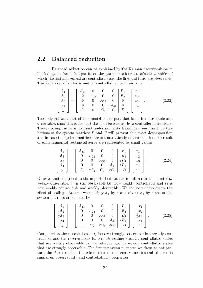
2.2 Balanced reduction

Balanced reduction can be explained by the Kalman decomposition inblock diagonal form, that partitions the system into four sets of state variables ofwhich the first and second are controllable and the first and third are observable.The fourth set of states is neither controllable nor observable

x1

x2

x3

x4

y

=

A11 0 0 0 B1

0 A22 0 0 B2

0 0 A33 0 00 0 0 A44 0C1 0 C3 0 D

x1

x2

x3

x4

u

. (2.23)

The only relevant part of this model is the part that is both controllable andobservable, since this is the part that can be effected by a controller in feedback.These decomposition is invariant under similarity transformation. Small pertur-bations of the system matrices B and C will prevent this exact decompositionand in case the system matrices are not analytically determined but the resultof some numerical routine all zeros are represented by small values

x1

x2

x3

x4

y

=

A11 0 0 0 B1

0 A22 0 0 B2

0 0 A33 0 εB3

0 0 0 A44 εB4

C1 εC2 C3 εC4 D

x1

x2

x3

x4

u

. (2.24)

Observe that compared to the unperturbed case x2 is still controllable but nowweakly observable, x3 is still observable but now weakly controllable and x4 isnow weakly controllable and weakly observable. We can now demonstrate theeffect of scaling. Assume we multiply x2 by ε and divide x3 by ε the scaledsystem matrices are defined by

x1

εx21ε x3

x4

y

=

A11 0 0 0 B1

0 A22 0 0 εB2

0 0 A33 0 B3

0 0 0 A44 εB4

C1 C2 εC3 εC4 D

x1

εx21εx3

x4

u

. (2.25)

Compared to the unscaled case x2 is now strongly observable but weakly con-trollable and the reverse holds for x3. By scaling strongly controllable statesthat are weakly observable can be interchanged by weakly controllable statesthat are strongly observable. For demonstration purposes we chose to not per-turb the A matrix but the effect of small non zero values instead of zeros issimilar on observability and controllability properties.

37

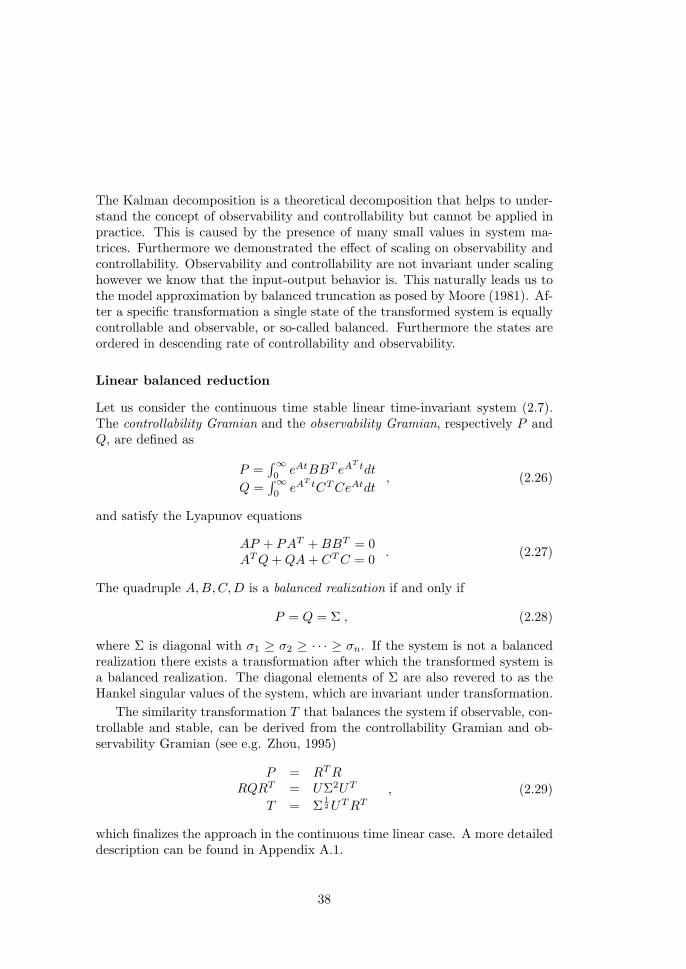
The Kalman decomposition is a theoretical decomposition that helps to under-stand the concept of observability and controllability but cannot be applied inpractice. This is caused by the presence of many small values in system ma-trices. Furthermore we demonstrated the effect of scaling on observability andcontrollability. Observability and controllability are not invariant under scalinghowever we know that the input-output behavior is. This naturally leads us tothe model approximation by balanced truncation as posed by Moore (1981). Af-ter a specific transformation a single state of the transformed system is equallycontrollable and observable, or so-called balanced. Furthermore the states areordered in descending rate of controllability and observability.

Linear balanced reduction

Let us consider the continuous time stable linear time-invariant system (2.7).The controllability Gramian and the observability Gramian, respectively P andQ, are defined as

P =∫∞0

eAtBBT eAT tdt

Q =∫∞0

eAT tCTCeAtdt

, (2.26)

and satisfy the Lyapunov equations

AP + PAT +BBT = 0ATQ+QA+ CTC = 0 . (2.27)

The quadruple A,B,C,D is a balanced realization if and only if

P = Q = Σ , (2.28)

where Σ is diagonal with σ1 ≥ σ2 ≥ · · · ≥ σn. If the system is not a balancedrealization there exists a transformation after which the transformed system isa balanced realization. The diagonal elements of Σ are also revered to as theHankel singular values of the system, which are invariant under transformation.

The similarity transformation T that balances the system if observable, con-trollable and stable, can be derived from the controllability Gramian and ob-servability Gramian (see e.g. Zhou, 1995)

P = RTRRQRT = UΣ2UT

T = Σ12UTRT

, (2.29)

which finalizes the approach in the continuous time linear case. A more detaileddescription can be found in Appendix A.1.

38

Since we will work in this chapter with discrete time models we also presentthe discrete time observability and controllability Gramian definitions. Let ustherefore define a discrete time model for the linear time invariant system definedin Equation (2.7) [

xk+1

yk

]=[

F GC D

] [xkuk

], (2.30)

where F and G are discrete transition matrices defined as

F = eAts and G =∫ ts

0

eA(ts−τ)Bdτ , (2.31)

for piece-wise constant (zero order hold) input signals and where ts is the sampleinterval.

For a discrete time linear system (2.30) the controllability and observabilityGramians are defined as

Wc = Σ∞k=0F

kGGTF kT

Wo = Σ∞k=0F

kTCTCF k, (2.32)

which satisfy the Lyapunov equations

FWcFT +BBT −Wc = 0

FTWoF + CTC −Wo = 0. (2.33)

The discrete time system defined by the system matrix quadruple F,G,C,D isbalanced if and only if

Wc =Wo = Σd , (2.34)

where Σd are the Hankel singular values of the discrete time system. In casea discrete system is not a balanced realization there exists a transformationafter which the transformed system is a balanced realization. This transforma-tion can be computed as described in Equations (2.29) but with discrete timecontrollability and observability Gramians.

The finite time discrete time controllability and observability Gramians aredefined as

Wc = ΣNk=0F

kGGTF kT

Wo = ΣNk=0F

kTCTCF k, (2.35)

where N is a big number instead of ∞. These Gramians are approximatesolutions of the Lyapunov Equations (2.33) and will be used later on in thischapter.

39

Numerical issues

The corresponding transformation for a balanced realization of the original sys-tem can be numerically ill conditioned. This is caused by the small Hankelsingular values that appear in the transformation matrix. Inversion of thesesmall Hankel singular values expose the addressed numerical problem. Thisproblem can be circumvented in case that we are only interested in the approxi-mate reduced model.

P = UcΣ2cU

Tc , (2.36)

Q = UoΣ2oU

To . (2.37)

Define the Hankel matrix

H := ΣoUTo UcΣc , (2.38)

and define the singular value decomposition of H

H = UHΣHV TH . (2.39)

Then the transformation matrix T is defined as

T := Σ12HV T

HΣ−1c UT

c , (2.40)

and inverse

T−1 = UcΣcVHΣ− 1

2H , (2.41)

or dually we can define T as

T := Σ− 12

H UTHΣoU

To , (2.42)

with inverse

T−1 = UoΣ−1o UHΣ

12H . (2.43)

Transformation T brings the system (2.7) into a balanced realization. Proof isby substitution of transformation matrices and Gramian decompositions of Pand Q in Lyapunov equations (2.27).

In case we are only interested in the reduced-order model we can derive awell conditioned projection[

z1

y

]=[

TLAT−1R TLB

CT−1R D

] [z1

u

], (2.44)

where

TL = Σ− 1

2H1

UTH1ΣoU

To , (2.45)

40

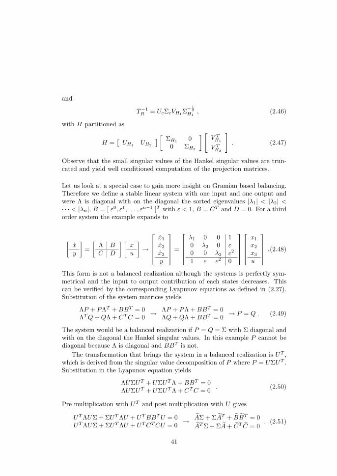
and

T−1R = UcΣcVH1Σ

− 12

H1, (2.46)

with H partitioned as

H =[UH1 UH2

] [ ΣH1 00 ΣH2

] [V TH1

V TH2

]. (2.47)

Observe that the small singular values of the Hankel singular values are trun-cated and yield well conditioned computation of the projection matrices.

Let us look at a special case to gain more insight on Gramian based balancing.Therefore we define a stable linear system with one input and one output andwere Λ is diagonal with on the diagonal the sorted eigenvalues |λ1| < |λ2| <· · · < |λn|, B = [ ε0, ε1, . . . , εn−1 ]T with ε < 1, B = CT and D = 0. For a thirdorder system the example expands to

[xy

]=[Λ BC D

] [xu

]→

x1

x2

x3

y

=

λ1 0 0 10 λ2 0 ε0 0 λ3 ε2

1 ε ε2 0

x1

x2

x3

u

.(2.48)

This form is not a balanced realization although the systems is perfectly sym-metrical and the input to output contribution of each states decreases. Thiscan be verified by the corresponding Lyapunov equations as defined in (2.27).Substitution of the system matrices yields

ΛP + PΛT +BBT = 0ΛTQ+QΛ + CTC = 0 → ΛP + PΛ +BBT = 0

ΛQ+QΛ +BBT = 0 → P = Q . (2.49)

The system would be a balanced realization if P = Q = Σ with Σ diagonal andwith on the diagonal the Hankel singular values. In this example P cannot bediagonal because Λ is diagonal and BBT is not.

The transformation that brings the system in a balanced realization is UT ,which is derived from the singular value decomposition of P where P = UΣUT .Substitution in the Lyapunov equation yields

ΛUΣUT + UΣUTΛ +BBT = 0ΛUΣUT + UΣUTΛ + CTC = 0 . (2.50)

Pre multiplication with UT and post multiplication with U gives

UTΛUΣ+ ΣUTΛU + UTBBTU = 0UTΛUΣ+ ΣUTΛU + UTCTCU = 0 → AΣ+ ΣAT + BBT = 0

ATΣ+ ΣA+ CT C = 0. (2.51)

41

The balanced realization is of the example is[zy

]=[

UTΛU UTBCU D

] [zu

]=

[A B

C D

] [zu

]. (2.52)

If ε 1 in the example U approaches the unity matrix and in that case theexample already is in a balanced realization.

Empirical Gramians

For linear systems we used Gramians to compute a balanced realization suitablefor model reduction by truncation. These Gramians are the solution of two Lya-punov equations that can be solved. For nonlinear systems we cannot deriveGramians in this way. The idea behind empirical Gramians is to derive Gra-mians from data generated by simulation. If it is possible to construct Gramiansfrom simulated data for linear systems the same technique can be applied tononlinear systems since simulation of a nonlinear system is possible. In this wayit would be possible to construct a Gramian that is associated to a nonlinearsystem.

Lall (1999) introduced the idea of empirical Gramians. Empirical Gramiamsare closely related to the covariance matrix introduced by Pallaske (1987)

M =∫G

∫ ∞

0

(x(t)− x∗)(x(t)− x∗)T dtdG , (2.53)

although Pallaske did not relate the approach to balancing. The symbol Gdenotes a set of trajectories resulting from a variation of initial conditions andinput signals. Loffler and Marquardt (1991) further elaborated the approachand suggested to use a set of step responses to generate data that represent thesystems dynamics.

Lall (1999) reconstructs the Gramians from data generated by either animpulse response, for the controllability Gramian, or response to an initial con-dition to derive the observability Gramian. Because of the orthogonality of theimpulses and initial conditions the data adds up to the controllability and ob-servability Gramian, respectively.

Lall defined the following sets for the empirical input Gramian:

T n = {T1, . . . , Tr | Tl ∈ Rn×n, TlT

Tl = I, l = 1, . . . , r}

M = {c1, . . . , cs | cm ∈ R+,m = 1, . . . , s}

En = {e1, . . . , en | standard unit vectors in Rn}

, (2.54)

where r is the number of different perturbation orientations, s is the number ofdifferent perturbation magnitudes and n is the number of inputs of the system

42

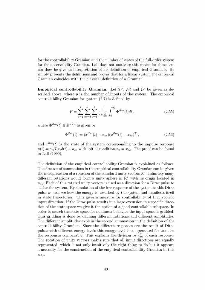
for the controllability Gramian and the number of states of the full-order systemfor the observability Gramian. Lall does not motivate this choice for these setsnor does he give an interpretation of his definition of empirical Gramians. Hesimply presents the definitions and proves that for a linear system the empiricalGramian coincides with the classical definition of a Gramian.

Empirical controllability Gramian. Let T p, M and Ep be given as de-scribed above, where p is the number of inputs of the system. The empiricalcontrollability Gramian for system (2.7) is defined by

P =r∑

l=1

s∑m=1

p∑i=1

1rsc2m

∫ ∞

0

Φilm(t)dt , (2.55)

where Φilm(t) ∈ Rn×n is given by

Φilm(t) := (xilm(t)− xss)(xilm(t)− xss)T , (2.56)

and xilm(t) is the state of the system corresponding to the impulse responseu(t) = cmTleiδ(t)+uss with initial condition x0 = xss. The proof can be foundin Lall (1999).

The definition of the empirical controllability Gramian is explained as follows.The first set of summations in the empirical controllability Gramian can be giventhe interpretation of a rotation of the standard unity vectors R

r. Infinitely manydifferent rotations would form a unity sphere in R

r with its origin located inuss. Each of this rotated unity vectors is used as a direction for a Dirac pulse toexcite the system. By simulation of the free response of the system to this Diracpulse we can see how the energy is absorbed by the system and manifests itselfin state trajectories. This gives a measure for controllability of that specificinput direction. If the Dirac pulse results in a large excursion in a specific direc-tion of the state space we give it the notion of a good controllable subspace. Inorder to search the state space for nonlinear behavior the input space is gridded.This gridding is done by defining different rotations and different amplitudes.The different amplitudes explain the second summation in the definition of thecontrollability Gramian. Since the different responses are the result of Diracpulses with different energy levels this energy level is compensated for to makethe responses comparable. This explains the division by c2m of each response.The rotation of unity vectors makes sure that all input directions are equallyrepresented, which is not only intuitively the right thing to do but it appearsa necessity for the construction of the empirical controllability Gramian in thisway.

43

Empirical observability Gramian. Let T n,M and En be given as describedabove, where n is the number of states of the original system. The empiricalobservability Gramian for system (2.7) is defined by

Q =r∑

l=1

s∑m=1

1rsc2m

∫ ∞

0

TlΨlm(t)TTl dt , (2.57)

where Ψlm(t) ∈ Rn×n is given by

Ψlmij (t) := (y

ilm(t)− yss)T (yjlm(t)− yss) , (2.58)

and yilm(t) is the output of the system corresponding to the initial conditionx0 = cmTlei + xss and yss is the steady-state value corresponding to the inputu(t) = uss. The proof can be found in Lall (1999).

The first set of summations in the empirical observability Gramian can be giventhe interpretation of a rotation of the standard unity vectors R

n. Infinitelymany different rotations would form a unity sphere in R

n with its origin locatedin the state state of the system. Each of this rotated unity vectors is used as aperturbation on the steady-state xss of the system. By simulation of the freeresponse of the system from this initial condition we can see how the energymanifests itself in the output. This gives a measure for observability of thatspecific direction in the state space. If it takes little energy to drive the systemin that direction of the state space and the energy strongly manifests itself in theoutput we give it the notion of a good controllable and observable subspace. Inorder to search the state space for nonlinear behavior the state space is gridded.This gridding is done by defining different rotations and different amplitudes.The different amplitudes are the second summation in the definition of the ob-servability Gramian. Since the different responses start with different energylevels this energy level is compensated for to make the responses comparable.The explains the division by c2m of each response. The rotation of unity vectorsmakes sure that all directions are equally represented, which is not only intui-tively the right thing to do but it appears a necessity for the construction of theempirical observability Gramian in this way.

Hahn et al. (2000) translated this to a discrete time version based on thesame definitions as Lall. Roughly speaking Hahn replaced the integral in theempirical Gramians by a finite sum approximation of the sampled continuoustime system, where xk is short hand notation for x|t=k∆t.

Discrete time empirical controllability Gramian. Let T p, M and Ep begiven as described above, where p is the number of inputs of the system. The

44

discrete time empirical controllability Gramian for system (2.30) is defined by

Wc =r∑

l=1

s∑m=1

p∑i=1

1rsc2m

q∑k=0

Φilmk , (2.59)

where Φilmk ∈ R

n×n is given by

Φilmk (t) := (xilmk − xss)(xilmk − xss)T , (2.60)

and xilmk is the state of the system corresponding to the impulse responseuk = cmTleiδk=0 + uss with initial condition x0 = xss.

Discrete time empirical observability Gramian. Let T n, M and En begiven as described above, where n is the number of states of the original system.The discrete time empirical observability Gramian for system (2.30) is definedby

Wo =r∑

l=1

s∑m=1

1rsc2m

q∑k=0

TlΨlmk TT

l , (2.61)

where Ψlmk ∈ R

n×n is given by

Ψlmij k

:= (yilmk − yss)T (yjlmk − yss) , (2.62)

and yilmk is the output of the system corresponding to the initial conditionx0 = cmTlei + xss and input uk = uss.

This approach enables to reconstruct discrete time Gramians from sampleddata. If this data is generated by a linear system the solution will convergeto the same solution as obtained by solving the Lyapunov equations (2.33).For data generated by a nonlinear system we end up with a so-called empiricalGramian. The empirical Gramian and the way Hahn derives it will be assessedlater in this chapter.

2.3 Proper orthogonal decomposition

Different names for proper orthogonal decomposition exist, such asKarhunen-Loeve expansion or method of empirical eigenfunctions. It providesa very effective way to compute low order approximate models. The idea of aproper orthogonal composition is to find an orthogonal transformation maxi-mizing the energy content in the first basis vectors. A common way to de-termine these optimal basis vectors (e.g. Aling et al., 1996; Shvartsman and

45

Kevrekidis, 1998) will be described next. For more references on this topic thereader is referred to the literature section in the previous chapter.

Let us execute a simulation with a model defined by Equations (2.1) andinput sequence u(t). Sampling the state trajectories of this simulation providesa so-called snapshot of the system

XN =[∆x(t0) ∆x(t1) . . . ∆x(tN )

], (2.63)

where ∆x(tk) = x(tk) − x∗ and x∗ is a steady state. The snapshot matrixXN ∈ R

nx×N with N � nx can be an ensemble of different simulations. Asingular value decomposition of XN is defined as

XN = UΣV T , (2.64)

where Σ is diagonal with σ1 ≥ σ2 ≥ · · · ≥ σn and with UUT = I and V V T = I.XN can be partitioned as

XN =[U1 U2

] [ Σ1 0 00 Σ2 0

] V T1

V T2

V T3

. (2.65)

Suppose that σmin(Σ1)� σmax(Σ2) we can assume Σ2 = 0, which implies that

XN = U1Σ1VT1

0 = U2Σ2VT2

. (2.66)

Apparently the transformation U distinguishes between two subspaces wheremost energy is captured by U1 and the rest of the energy is gathered in U2. Letus define a new coordinate system[

z1(t)z2(t)

]=[

UT1

UT2

](x(t)− x∗) . (2.67)

The set of ordinary differential equations defined by Equations (2.1) can bereduced by transformation and truncation[

z1

y

]=[

UT1 f(U1z1 + x∗, u)g(U1z1 + x∗, u)

],

z1(t0) = UT1 (x0 − x∗)

z2 = 0 . (2.68)

Or without elimination of x in the right hand side, which can be practical froman implementation point of view x

z1

y

= U1z1 + x∗

UT1 f(x, u)g(x, u)

,z1(t0) = UT

1 (x0 − x∗)z2 = 0 . (2.69)

46

The same transformation can be used to reduce the model by residualization z1

0y

= UT

1 f(U1z1 + U2z2 + x∗, u)UT

2 f(U1z1 + U2z2 + x∗, u)g(U1z1 + U2z2 + x∗, u)

, z1(t0) = UT1 (x0 − x∗) , (2.70)

which is equivalent toz1

0yx

=

UT1 f(x, u)

UT2 f(x, u)g(x, u)

Uz + x∗

, z1(t0) = UT1 (x0 − x∗) . (2.71)

Recall that in case of residualization we reduce the number of differential equa-tions transforming the set of ordinary differential equations (ode) into a set ofdifferential and algebraic equations (dae).

Proper orthogonal decomposition revised

State transformation and scaling before applying the singular value decomposi-tion has a decisive effect on the transformation and thus reduction of the model.

XN =WXN =WUΣV T . (2.72)

A state coordinate change has a major effect on the model reduction. This isan important observation:

Reduction by means of proper orthogonal decompositionstrongly depends on specific choice of coordinate system.

This can be proven by a special choice ofW = Σ−1UT , which yields a coordinatesystem where all states are equally important,

XN =WUΣV T = Σ−1UTUΣV T = U ΣV T , (2.73)

with U = I ∈ Rnx×nx and Σ = I ∈ R

nx×N .A pragmatic solution is scaling with a matrix with only on its diagonal the

reciprocal of the difference between maximal and minimal allowable value forthat specific variable. In this way all variables are normalized and differences inunits are compensated for. Most successes reported in papers on model reduc-tion with proper orthogonal projection consider discretized partial differentialequations with only one type of variable (e.g. only temperatures). When amodel consists variables with different units their relative importance dependson the specific choice of units. Proper orthogonal decomposition applied to amodel involving temperatures and mass, where mass is expressed in kilograms

47

and temperatures in degrees Kelvin, will give other results than the same modelwith mass expressed in tons.

Computation of the singular value decomposition of a snapshot can be quitedemanding. This is caused mainly by the computation of V T , which is a N ×Nmatrix with N very large. In case we are only interested in the orthogonalprojection matrix U we can reduce the computation load by computation of thesingular value decomposition of XNXT

N ,

XNXTN = UΣV TV ΣUT = UΣ2UT . (2.74)

In this way we do not compute V T and still have access to the projection matrixU and the corresponding singular values Σ.

The data for the snapshot matrix is generated by simulation of the modelwith a specific choice of inputs. Transformation based on this snapshot stronglydepends on the choice of input signals. White noise input signals on all inputchannels does not discriminate between high and low frequency content andwill excite the model without preference. In case one has information on whatfrequency range is relevant for the model to approximate we can put more energyin this part of the input signal, which results in a better approximation in thisfrequency range. In case we have a clear idea what the relevant input signalslook like we can fine tune the model reduction to this set of input signals. Thismost probably allows for a larger degree of model reduction. However, for signalsnot represented in the set input signals used for generation of the snapshots wecannot expect good performance of the reduced model. So depending of theknowledge on future input signals this property can either be an advantage ora disadvantage.

In case a model based optimization is used to explore new optimal trajecto-ries we do not know how the input trajectories look like. In that case we haveto resort to some white random type of input signals, most probably still allow-ing for a certain degree of reduction. One can think of the weakly controllablestates. Regardless of the choice of inputs, these states will only get little energyfrom the inputs and will be reduced in this approach anyway. The discrete timecontrollability Gramian and snapshot matrix are strongly related in case thatwhite noise inputs are used,

XNXTN = N ·Wc = N · UcΣ2

cUTc , (2.75)

with N the number of samples in the snapshot matrix,Wc the discrete time con-trollability Gramian and Uc and Σ2

c the orthogonal matrix and singular valuematrix of the controllability Gramian, respectively. Note that the transforma-tion matrix used for proper orthogonal projection coincides with the singularvalue decomposition of the controllability Gramian. See Appendix B for details.

In case another than white noise signal is used to generate the snapshotmatrix we can consider this as the result of a filtered white noise signal. This

48

brings us into the topic of so-called frequency balanced reduction. See for detailson frequency weighted balanced reduction e.g. Wortelboer (1994). Frequencyanalysis of the input signals used to generate the snapshot matrix will provideinsight in what frequency ranges the model is excited. All input data without awhite spectrum indicate some kind of frequency weighting. So the observationis that:

For a linear system a snapshot matrix times its transpose approximatesthe (frequency weighted) discrete time controllability Gramian.

Dynamics related to input directions and frequency ranges that are not excitedwill not be present in the data and therefore will be removed from the model.This is not a model property but a the result of input signal selection. Notethat a model itself acts as a filter, so in case two units are in a series connectionthe first acts as a filter on signals that are applied to the first unit before theyare affecting the second unit. Even more interesting is it when the output ofthe second unit affects the first unit by means of a material recycle streamor feedback control. Although the above reasoning is based on linear modelproperties for smooth nonlinear systems we can argue that a similar reasoningholds.

Singular values can provide information on the possible model order reduc-tion. However, model stability is a more important property of the reducedmodel. Unfortunately no guarantees exist for stability of projected nonlinearmodels. Even stronger, a lower order reduced model can be stable for a specifictrajectory whereas a higher order reduced model becomes unstable for the sametrajectory. In Chapter 5 will be elaborate on this issue.

Loffler and Marquardt (1991) motivated and applied a weighted Euclidiannorm ‖ · ‖Q defined as

‖x‖Q = xTQTQx , (2.76)

with a positive definite and quadratic weighting matrix Q. The covariancematrix defined in Equation (2.53) can be written as

M =∫G

∫ ∞

0

Q(x(t)− x∗)(x(t)− x∗)TQT dtdG . (2.77)

This weighted covariance matrix can be approximated by QXNXTNQT and

shows that model reduction by a weighted proper orthogonal decompositionis strongly related to model reduction based on the covariation matrix M . IfG consists of the same set of simulations that generated XN , reduction basedproper orthogonal decomposition and reduction based on the covariance matrixwill be almost identical.

49

In this chapter two important model reduction techniques from literature werediscussed and given an interpretation. We will now proceed with a reformula-tion of the empirical Gramian in a new format that is more flexible and moreinsightful than the empirical Gramians previously defined in this chapter.

2.4 Balanced reduction revisited

In this section we will focus on properties and interpretation of empiricalGramians and how these are derived. First we will formulate a more simpleway to derive discrete time empirical Gramians as introduced by Lall (1999).This will be referred to as perturbed data based empirical Gramians. Thisformulation allows for a more flexible way how to derive empirical Gramians.Then this formulation is extended to a generalized formulation that allows for aderivation of empirical Gramians with almost arbitrary input trajectories. Thiswill be referred to as the generalized empirical Gramians. Finally we will explainhow to interpret the empirical Gramian by means of a simple example revealingthe true mechanism behind empirical Gramians.

From a theoretical point of view balanced reduction using Gramians is pre-ferred over reduction by orthogonal decomposition since it really takes intoaccount the model contribution between input and output and does not de-pend on internal coordinate system (see previous section). The affect of scalingof selected inputs and outputs on the reduced model can qualitatively be pre-dicted with common engineering sense. Scaling of the states is still preferablebut only from a numerical conditioning point of view. Theoretically a statetransformation does not affect the result of balanced model reduction.

Discrete time perturbed data based Gramians

Gramians can be reconstructed from data generated by perturbation of thesteady-state of a linear discrete time system. For the empirical observabilityGramian we need to perturb the initial condition in different directions andsimulate the free response to is equilibrium. For the empirical controllabilityGramian we apply Dirac pulses in different directions via the inputs and simu-late the free responses. This was the basis on which the empirical Gramians byLall (1999) were defined. The constraint that is enforced by Lall is that each setof perturbations is orthogonal. This constraint is crucial for the computation ofthe empirical Gramians as formulated in his way. This restriction is somewhatartificial and can be very unpractical and above all is unnecessary as we willdemonstrate next.

50

For this reformulation new data matrices are required and these are definednext. Suppose a stable linear discrete time system as defined in (2.30) is inequilibrium with u∗ = 0 and therefore x∗ = 0. Let us define YN as an outputresponse data matrix

YN =

y10 y2

0 · · · yp0y11 y2

1 · · · yp1...

......

y1q y2

q · · · ypq

, (2.78)

where yrk is the value of the output at time t = kh and k = {0, . . . , q} of therth free response observed in the output. This free response is the result of aperturbed initial condition xr0. All perturbed initial conditions are stacked in asecond matrix X0 defined as

X0 =[x1

0 x20 · · · xp0

]. (2.79)

With the definition of YN and X0 we defined the two matrices required tocompute the discrete time perturbed data based observability Gramian.

Discrete time perturbed data based observability Gramian

Let YN and X0 be given as described above. The data based discrete timeobservability Gramian as defined in Equation (2.32) for the discrete time linearsystem as defined in Equation (2.30) is

Wo = X†0

TY TN YNX†

0 , (2.80)

where X†0 is a right inverse of X0

X†0 = XT

0 (X0XT0 )

−1 . (2.81)

Proof:

The output data matrix YN can be written as

YN = ΓoX0 , (2.82)

with Γo the discrete time observability matrix

Γo =

CCF...

CF q

. (2.83)

51

Substitution yields

Wo = X†0

TXT

0 ΓTo ΓoX0X

†0 = Γ

To Γo (2.84)

=[CT FTCT F qTCT

]

CCF...

CF q

(2.85)

= Σqk=0F

kTCTCF k . (2.86)

The proof ends by letting q → ∞.

Now we can link this formulation to the formulation used by Hahn. Supposethat the we have as many initial conditions as states and that these initialconditions are orthonormal. The advantage of this orthonormality is that wedo not need to compute the inverse of X0X

T0 since this is by definition equal to

the unity matrix. This knowledge is exploited in the formulation used by Hahn.By substitution of X0X

T0 = I into Equations (2.81) and (2.80) we can recognize

the formulation by Hahn presented in Equation (2.61)

Wo = X0YTN YNXT

0 . (2.87)

We only need to convert the matrix notation into a summation representation.The full proof that the formulation by Hahn fits within the new formulation canbe found in Appendix A.2. The price we have to pay in this new definition isthat we need to compute the pseudo inverse X†

0 but in return we may plug inany initial condition we would like, which obviously is less restrictive. The newconstraint is that the conditioning ofX0X

T0 should allow for a numerically stable

inversion, which is less restrictive than enforcing orthogonality. Furthermore wecan add extra initial conditions one by one instead of by a whole orthogonalset at once. The different amplitudes and the number of initial conditions aredirectly accounted for.

In a similar way we can derive the discrete time perturbed data based con-trollability Gramian. Let us define XN as the state response data matrix

XN =[X1

N X2N · · · Xp

N

], (2.88)

where

XrN =

[xr1 xr2 · · · xrq

], (2.89)

and xrk is the value of the state at t = kh of the impulse response to ur0. DefineU0 as the matrix with all impulse values

U0 =[U1

0 U20 · · · Up

0

], (2.90)

52

where

Ur0 =

ur0 0 00 ur0 0

. . .0 0 ur0

, (2.91)

such that

XrN = ΓcUr

0 , (2.92)

with the discrete time controllability matrix

Γc =[G FG · · · F qG

]. (2.93)

Discrete time perturbed data based controllability Gramian

Let XN and U0 be given as described above. The data based discrete timecontrollability Gramian as defined in Equation (2.32) for the discrete time linearsystem as defined in Equation (2.30) is

Wc = XNU†0U

†0

TXT

N , (2.94)

where U†0 is the right inverse of U0

U†0 = UT

0 (U0UT0 )

−1 . (2.95)

Proof:

The state response matrix XN can be written as

XN = ΓcU0 . (2.96)

Substitution yields

Wc = ΓcU0U†0U

†0

TUT

0 ΓTc = ΓcΓ

Tc (2.97)

=[G FG · · · F qG

]

GT

GTFT

...GTF qT

(2.98)

= Σqk=0F

kGGTF kT . (2.99)

The proof ends by letting q → ∞.

53

ζ1

ζ2 Rp

ζ1

ζ2 Rp

Figure 2.1: Left: favorable steady-state with maximum perturbation radiuswhere ζ represent either states in R

nx or inputs in Rnu. Right: steady-state

near a constraint results in a smaller admissible radius of feasible perturbations.

Again we can link this formulation to the formulation adopted by Hahn. Sup-pose we have as many impulse responses as inputs and these impulses hap-pen to be orthonormal, which is required within Hahn’s framework. In thatcase we know that by definition U0U

T0 = I. By substitution of U0U

T0 = I in

Equations (2.95) and (2.94) we already can recognize the formulation by Hahnpresented in Equation (2.59)

Wc = XNU0UT0 XT

N = XNXTN . (2.100)

We only need to convert the matrix notation to a summation representation.Most of all pros and cons that apply to the empirical observability Gramianapply to the empirical controllability Gramian. So, in the new formulationwe can add one input perturbation at a time in an arbitrary direction andmagnitude as long as the conditioning of U0U

T0 allows for a numerical stable

computation of the right inverse. This is a much more flexible formulation andenables easy computation.

Note the resemblance between Equation (2.100) and snapshot matrix used todo proper orthogonal decomposition in Equation (2.75). For special choices ofsignals the snapshot matrix times its transpose is identical to the controllabilityGramian.

So the empirical Gramians as defined by Lall (1999) and adopted by Hahnet al. (2000) are a special case of the Gramians presented in this section. If theperturbations are chosen as orthogonal sets with possibly different amplitudesthe two methods coincide. However, since there is no fundamental motivationfor this choice, other than numerical reasons, the method as presented in thissection leaves more freedom for the user to choose perturbations. The onlycondition on the perturbations is that they should span the whole column space.

54

A practical disadvantage of the orthogonal perturbations as proposed by Lall(1999), is related to constraints on perturbations. These constraints come na-tural with the model such as positiveness of variables and (molar) fractions thatshould remain between zero and one. This is illustrated in Figure 2.1 wherein the left picture the steady-state is chosen such that a large area of the ad-missible perturbations can be covered by orthogonal sets of perturbations. Inthe right of the same figure is illustrated that a constraint near the steady-staterestricts the radius of admissible perturbations. In case of the method presentedin this section the perturbations can freely be chosen as long as they satisfy theconstraints and span the whole space. Note that the illustration holds for inputperturbations as well as for state perturbations.

It is questionable if the relevant nonlinear dynamics are revealed with thisperturbation approach. This observation inspired to develop a method thatenables computation of empirical Gramians from a single simulation of a rele-vant trajectory. It is closely related to the discrete time perturbed data basedGramians introduced in this section.

Generalized data based Gramians

The data based Gramians in the previous section are constructed from impulseresponse data and data from perturbation of steady-state conditions. In thissection we will generalize this to a much wider class of signals. We will presenthow to use data from one simulation of a trajectory for the construction ofboth controllability and observability Gramian. We will demonstrate how theapproach is applied to an asymptotically stable linear model which is assumedto be in steady-state at the beginning of the trajectory.

Let us define the data matrix XN as the snapshot matrix of the matrix

XN =[x1 x2 · · · xN

], (2.101)

where xk is the value of the state at t = kh of the response to the input sequenceu(t). The covariance matrix M =

∫G∫ tN0(x(t)−x∗)(x(t)−x∗)T dtdG as used by

Loffler and Marquardt (1991) can be approximated by XNXTN . The covariance

matrix does not equal the observability or controllability Gramian. Only if Gis chosen in the special way (orthogonal impulse responses) as defined in Lall(1999), the covariance matrix will approximate the controllability Gramian.

XN can be written as

XN = ΓNc UNN , (2.102)

with ΓNc the discrete time controllability matrix

ΓNc =[G FG · · · FNG

], (2.103)

55

and the input matrix UNN defined as

UNN =

u0 u1 · · · uN0 u0 · · · uN−1

.... . . . . .

...0 · · · 0 u0

. (2.104)

If the system is stable limq→∞ F q = 0. Therefore we can truncate the control-lability matrix and input matrix and approximate XN

XN ≈ ΓcUN , (2.105)

with Γc the truncated controllability matrix as in Equation (2.93) and the trun-cated input matrix as

UN =

u0 u1 · · · uq uN−1

0 u0 · · · uq−1 uN−2

.... . . . . .

...0 · · · 0 u0 uN−1−q

. (2.106)

Generalized discrete time data based controllability Gramian

Let XN and UN be given as described above. The data based discrete timecontrollability Gramian for the discrete time linear system (2.30) is defined by

Wc = XNU†NU†

N

TXT

N , (2.107)

where U†N is the right inverse of UN

U†N = UT

N (UNUTN )

−1 . (2.108)

Proof:

The state response matrix XN can be written as

XN = ΓcUN (2.109)

Substitution yields

Wc = ΓcUNU†NU†

N

TUTNΓ

Tc = ΓcΓ

Tc (2.110)

=[G FG · · · F qG

]

GT

GTFT

...GTF qT

(2.111)

= Σqk=0F

kGGTF kT , (2.112)

56

which completes the proof.

For the observability Gramian we use the Hankel matrix. Let us define theoutput data matrix YN as

YN =[y1 y2 · · · yN

], (2.113)

with the argument that limq→∞ F q = 0 YN can be approximated by

YN ≈ ΓcoUN , (2.114)

with the truncated Markov parameters Γco defined as

Γco =[CG CFG · · · CF 2qG

], (2.115)

and UN is the truncated input matrix. The Markov parameters can be deter-mined by

Γco = YNU†N , (2.116)

with U†N the right inverse of UN as defined in Equation (2.108). The Hankel

matrix is defined as

H = ΓoΓc =

CG CFG · · · CF qG

CFG...

......

CF qG · · · · · · CF 2qG

, (2.117)

which can be filled with the Markov parameters.

Generalized discrete time data based observability Gramian

Let H and Γc be defined as described above. The data based discrete timeobservability Gramian for the discrete time linear system (2.30) is defined by

Wo = Γ†c

THTHÆ

c , (2.118)

with Γ†c as the right inverse of Γc

Γ†c = Γ

Tc (ΓcΓ

Tc )

−1 = ΓTc W−1c . (2.119)

57

Proof:

Substitution of H yields

Wo = Γ†c

TΓTc Γ

To ΓoΓcΓ

†c = Γ

To Γo (2.120)

=[CT FTCT F qTCT

]

CCF...

CF q

(2.121)

= Σqk=0F

kTCTCF k , (2.122)

which completes the proof.

The right inverses used in the computation of the Gramians must exist andshould be well conditioned. In case of the right inverse of the input matrix UN

this can be achieved by a proper choice of inputs whereas the existence and wellconditioned right inverse of Γc cannot be guaranteed. This issue will be treatedin an example in the next section. First we will reveal the underling mechanismof empirical Gramians. Basic question was what an empirical Gramian lookedlike if data was gathered in two different operating conditions of a nonlinearsystem using small perturbations. The use of small perturbations implies thatonly the local linear behavior of the nonlinear model is excited.

Example of two linear models

We will investigate the mechanisms that occur in the case of computation ofempirical Gramians. Therefore we assume two linear discrete time systems thatrepresent the local dynamics of a nonlinear system in two different operatingpoints [

F1 G1

C1 0

],

[F2 G2

C2 0

].

The according controllability Gramians are

Wc1 = Γc1ΓTc1 =[G1 F1G1 . . . F q

1G1

]

GT1

GT1 F

T1

...GT

1 Fq1T

,

58

and

Wc2 = Γc2ΓTc2 =[G2 F2G2 . . . F q

2G2

]

GT2

GT2 F

T2

...GT

2 Fq2T

.

We can generate data in these two points that we collect in data matrices XN1

and XN2, respectively

XN1 = Γc1UN1, XN2 = Γc2UN2 .

We already proved the local controllability matrix can be reconstructed fromthis data and therefore the the controllability Gramian as well. The two localcontrollability matrices are

Γc1 = XN1UTN1(UN1U

TN1)

−1

Γc2 = XN2UTN2(UN2U

TN2)

−1 .

Substitution of XN1 and XN2 yields

Γc1 = Γc1UN1UTN1(UN1U

TN1)

−1

Γc2 = Γc2UN2UTN2(UN2U

TN2)

−1 .

Suppose we computed the average controllability matrix by combining the twodata sets

UN =[UN1 UN2

]XN =

[XN1 XN2

]=[Γc1 Γc2

] [ UN1 00 UN2

]= ΓcUN .

Solution for this average controllability matrix Γc is

Γc = XNUTN (UNUT

N )−1 .

Substitution of XN and UN yields

Γc =[Γc1 Γc2

] [ UN1 00 UN2

] UTN1

UTN2

[ UN1 UN2

] UTN1

UTN2

−1

=[Γc1 Γc2

] UN1UTN1

UN2UTN2

[ UN1UTN1 + UN2U

TN2

]−1.

59

Suppose UN2 = γUN1. This implies that we use identical input signals for datageneration in the second operating point as were used for data generation in thefirst operating point but scaled with the contstant γ. Substitution yields

Γc =[Γc1 Γc2

] UN1UTN1

γ2UN1UTN1

[ UN1UTN1 + γ2UN1U

TN1

]−1

=1

1 + γ2

[Γc1 Γc2

] [ Iγ2I

]=

11 + γ2

Γc1 +γ2

1 + γ2Γc2 .

If γ = 1, so if we use exactly the same inputs signals, we see that the interpolatedcontrollability matrix coincides with the equally weighted interpolation of thetwo local controllability matrices

Γc =12(Γc1 + Γc2) .

An other special case is when UN1UTN1 = α2I and UN2U

TN2 = β2I. This is the

case if we apply an energy level of α2 to the to the first operating point and β2

to the second operating point. The perturbation orientation and amplitude inboth operating points are completely free as long as they can be described byorthogonal sets of perturbations. Substitution yields

Γc =[Γc1 Γc2

] [ α2Iβ2I

] [α2I + β2I

]−1

=1

α2 + β2

[Γc1 Γc2

] [ α2Iβ2I

]=

α2

α2 + β2Γc1 +

β2

α2 + β2Γc2 .

So by allocation of energy in the test signals over operating points we emphasizedifferent operating points. If we want to compute the empirical Gramian basedon data generated in two operating points and use small perturbations this issimilar to averaging of the two controllability matrices. This is not equal toaveraging the two controllability Gramians. The proof is simple

Wc = 12Wc1 + 1

2Wc2 = 12Γc1Γ

Tc1 +

12Γc2Γ

Tc2 , (2.123)

�=ΓcΓTc =

14Γc1Γ

Tc1 +

14Γc1Γ

Tc2 +

14Γc1Γ

Tc2 +

14Γc2Γ

Tc2 . (2.124)

One could argue that this is a flaw of the empirical Gramian. This concludesthe true underlying mechanism of the Empirical Gramians.

60

Interpolation of local linear Gramians

Motivated by the conclusion that in the end empirical Gramians attempt toreconstruct Gramians of local linear dynamics a simple alternative for the databased Gramians is interpolation of local Gramians. Loffler and Marquardt(1991) approximated the covariance matrix as defined in Equation (2.53) byusing multiple linear models. The covariance matrix was computed directly bymeans of a Monte Carlo method and using the linear approximation.

Interpolation of local Gramians is done by deriving a number of linear modelsin a relevant operating range from which the local Gramians can be computedby solving the discrete time Lyapunov equations (2.33). This yields

Wc =1N

N∑i=1

Wc,i , (2.125)

and

Wo =1N

N∑i=1

Wo,i , (2.126)

where Wc,i and Wo,i are the local controllability and observability Gramian,respectively. The local Gramians can be weighted with γ to emphasize specificoperating points. This yields

Wc =1∑N

i=1 γc,i

N∑i=1

γc,iWc,i , (2.127)

and

Wo =1∑N

i=1 γo,i

N∑i=1

γo,iWo,i . (2.128)

The result of this averaging approximates the perturbed data based Gramiansin case the effect finite data is negligible and sufficiently small perturbations areused.

61

2.5 Evaluation on a process model

In this chapter different ways to compute Gramians were presented.In this section we will compare different approaches by applying them to asimple model. In the first test we want to exclude nonlinear effects to enablea lucent assessment of the different data based empirical reduction techniquesby using a linearization of a nonlinear model. In the next tests we return tothe nonlinear model we will then compare different Gramian based reductionapproaches where we focus on differences between data based Gramians andGramians derived from linearizations of the nonlinear model.

....................................................................... ...........................................

............................

.......................................................................

.......................................................................

.......................................................................

....................................................................... ...........................................

............................

.......................................................................

.......................................................................

.......................................................................

...............................................................

...............................................................

.....................................................................................................................

.....................................................................................................................

✠❄

✲

✲

❄❄

✲

✲

✒

✛ ............................................................................................................................................................

Figure 2.2: Schematic of the process model: reactor in series with a distillationcolumn with recycle to the reactor.

In this chapter we propose to use a simple model of a plant. A schematic ofthat plant is presented in Figure 2.2. The process represent a general classof chemical processes consisting of a reactor with separation unit and recyclestream. All levels are controlled and the top and bottom quality are measuredand controlled by reflux ratio and boilup rate, respectively. Temperate in thereactor is assumed to be constant by tight temperature control. For detailedmodel information the reader is referred to Chapter 3 for a general descriptionand Chapter 4 for details on modelling assumptions.

The model consists of 24 differential equations1 and we are interested in thetop purity and bottom impurity that are controlled by reflux ratio and boiluprate. So by model reduction we want to find a low order model that still properlyrepresents the input to output dynamics. Note that the effect of the reactor istaken into account since the reactor is connected to the column by fresh feedand recycle stream.

1gproms code can be found on the webpage http://www.dcsc.tudelft.nl/Research/Software.

62

xk+1 = Fxk + Guk

yk = Cxk + Duk

W dc

W do

(2.32)

(2.32)

W qc

W qo

(2.35)

(2.35)

W ec

W eo

(2.59)

(2.61)

W gc

W go

(2.107)

(2.118)

Ld

Rd

Lq

Rq

Le

Re

Lg

Rg✲

✲

✲

✲

✲

✲

✲

✲✲

Figure 2.3: Schematic overview of projections based on different Gramians withbetween brackets the corresponding equation numbers.

Results on the linearized model

For the linear model the bottom impurity and top purity are used as outputs, y1

and y2, respectively, and reflux ratio and boilup rate are used as inputs, u1 andu2, respectively. In this thesis we restrict to piecewise constant input signalsand therefore it is sensible to use discrete time Gramians instead of continuoustime Gramians. In this way the choice for the limited class of possible inputsignals enters the Gramians and consequently into the projections. Moore (1981)elaborates in his paper on the effect of sample time on discrete time Gramiansand the relation to the continuous time Gramian.

In Figure 2.3 all different projections that will be considered in the first testare presented in a schematic way. Wc and Wo are controllability and observa-bility matrices with superscripts d for discrete-time (Equation 2.32), q for finitediscrete-time (Equation 2.35), e for empirical (Equations 2.59 and 2.61) andq for generalized (Equations 2.107 and 2.118), respectively. L and R are the leftand right projectors derived from the Gramians and result in the reduced-ordermodel by truncation.

In Figure 2.4, the norm of the error, defined as

‖G(s)− G(s)‖ , (2.129)

of the reduced-order models based on the four different Gramians (exact, finitetime, empirical and generalized, respectively) is plotted against the reducedmodel order. It is hard to discriminate between the reduced models for mostorders since the approximation error is of the same order of magnitude. Theoret-ically the results should coincide except for the exact discrete-time solution. The

63

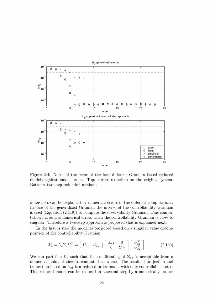
0 5 10 15 20 25

10−8

10−6

10−4

10−2H2 approximation error

||ε|| 2

order

0 5 10 15 20 25

10−8

10−6

10−4

10−2H2 approximation error 2 step approach

||ε|| 2

order

exactfiniteempiricalgeneralized

Figure 2.4: Norm of the error of the four different Gramian based reducedmodels against model order. Top: direct reduction on the original system.Bottom: two step reduction method.

differences can be explained by numerical errors in the different computations.In case of the generalized Gramian the inverse of the controllability Gramianis used (Equation (2.119)) to compute the observability Gramian. This compu-tation introduces numerical errors when the controllability Gramian is close tosingular. Therefore a two-step approach is proposed that is explained next.

In the first is step the model is projected based on a singular value decom-position of the controllability Gramian

Wc = UcΣcUTc =

[Uc1 Uc2

] [ Σc1 00 Σc2

] [UTc1

UTc2

]. (2.130)

We can partition Uc such that the conditioning of Σc1 is acceptable from anumerical point of view to compute its inverse. The result of projection andtruncation based on Uc1 is a reduced-order model with only controllable states.This reduced model can be reduced in a second step by a numerically proper

64

balanced reduction. In this example the first reduction resulted in a reducedmodel of order eight. Therefore in the bottom of Figure 2.4 only the errors ofthe balanced reduced models up to the order of eight are present. This two-stepapproach does not work in general and it is possible to come up with an exampleto prove this. In practice it provides a suitable reduction as we will see.

The dashed line in Figure 2.4 represent a user defined error level of 10−3. Wecan see in the top of this figure that we need three orders to meet that boundexcept for the generalized empirical Gramian reduced-order model that needsfive orders. In case of the two step approach we see at the bottom of Figure 2.4the same result except that for the generalized empirical Gramian we need fourorders instead of five. This is the effect of better numerical properties of thecomputations.

A different way to assess the quality of the reduced models is to compare stepresponses. Step responses of these models are depicted in Figures 2.5 and 2.6.Note that the steady state values of the nonlinear model for the bottom impuritywere 0.01 and 0.90 for the top purity and that the reduced linear models only arevalid close to this operating point. The two successive projections do not affectthe reduction up to the fifth order for all Gramians except for the generalizedGramian. The reduced models derived from the generalized empirical Gramiansimprove by applying the two successive projections: the fourth order model inFigure 2.6 is better than the fifth order model in Figure 2.5. This conclusioncan also be drawn from Figure 2.4 where the error of the fifth order model inthe top of the figure is larger than the error of the forth order computed by thetwo-step approach.

The results illustrate that both data based methods to derive Gramiansenable a balanced reduction that approximates the balanced reduction based onthe Gramian that is the solution of the Lyapunov equation. The computationsthat are involved in case of the generalized empirical observability Gramianare sensitive to the conditioning of the controllability Gramian and therefore atwo-step reduction approach was introduced.

Results on the nonlinear model

For nonlinear models we know that the controllability and observability dependon the point of operation. Therefore we need to make sure that only data isproduced that represent the operating envelope of interest. This is not trivialbut we can think of different possible scenarios. In Figure 2.7 four differentapproaches are presented to cover the relevant operating envelope.

In the situation indicated with the capital roman number I it is illustratedthat we compute some average operating point from which the system is per-turbed such that both steady-states A and B are enclosed by these unit ballperturbations. Besides a number of practical problems that can occur, such as

65

0 10 20 30 40−0.01

−0.008

−0.006

−0.004

−0.002

0u(1)

time [hr]

y(1)

0 10 20 30 40−4

−3

−2

−1

0x 10−3 u(2)

time [hr]

y(1)

0 10 20 30 40−0.14

−0.12

−0.1

−0.08

−0.06

−0.04

−0.02

0u(1)

time [hr]

y(2)

0 10 20 30 400

0.02

0.04

0.06

0.08

0.1

0.12

0.14u(2)

time [hr]

y(2)

Step Response

Ampl

itude

org−24redq−3rede−3redg−5

Figure 2.5: Full order linear model and reduced models based on different Gra-mians. Boilup rate and reflux rate are inputs u(1) and u(2), respectively andbottom impurity and top purity are outputs y(1) and y(2), respectively.

0 10 20 30 40−0.01

−0.008

−0.006

−0.004

−0.002

0u(1)

time [hr]

y(1)

0 10 20 30 40−4

−3

−2

−1

0x 10−3 u(2)

time [hr]

y(1)

0 10 20 30 40−0.14

−0.12

−0.1

−0.08

−0.06

−0.04

−0.02

0u(1)

time [hr]

y(2)

0 10 20 30 400

0.02

0.04

0.06

0.08

0.1

0.12

0.14u(2)

time [hr]

y(2)

Step Response

Ampl

itude

org−24redq−3rede−3redg−4

Figure 2.6: Full order linear model and reduced models based on two successiveprojections. Boilup rate and reflux rate are inputs u(1) and u(2), respectivelyand bottom impurity and top purity are outputs y(1) and y(2), respectively.

66

Rnx

A

B

I

.........................................................................

..................................................................................................................................................................................................

..................................................

Rnx

A

B

II

.........................................................................

..................................................................................................................................................................................................

..................................................

Rnx

A

B

III

.........................................................................

..................................................................................................................................................................................................

..................................................

Rnx

A

B

IV

Figure 2.7: Four different approaches to cover the relevant state space operatingenvelope between the two stationary operating points, i.e. 0 = f(x, u), A andB in R

nx . The solid line represents a trajectory that satisfies x = f(x, u).

e.g. the presence of constraints that restrict the radius of admissible pertur-bations, it is very questionable whether this approach represents the relevantoperating envelope. By increasing the operating envelope the validity require-ments for the model increase, which reduces the potential for model reduction.Therefore the operating envelope should be large enough to capture all relevantdynamics but also as small as possible to exclude all non-relevant dynamics.

In the situation indicated by the capital roman number II it is illustratedthat we restrict to small perturbations in the two steady-states A and B. Thisis implementable since we can decrease the perturbations until all constraintviolations have disappeared. Note however, that for small perturbations alldata based Gramians converge to the two stationary Gramians that can also becomputed by derivation of a linear model and solving two Lyapunov equations.The empirical Gramian is derived from the united data sets derived in the twosteady-states A and B. Note that in case we use sufficiently small perturbationsand an equal number of perturbations in both steady-states, computation of em-pirical Gramians approximates the average Gramian of the two local Gramians.Drawback of this approach can be the area covered by the perturbations doesnot cover the whole transition between steady-states A and B. This naturallybrings us to the situation that is depicted in Figure 2.7 with the capital romannumber III.

67

1.8 2 2.2 2.4 2.6 2.8 3 3.2 3.4 3.6 3.8

1.2

1.4

1.6

1.8

2

2.2

2.4

2.6

2.8

3

3.2input perturbations

boilup rate

reflu

x ra

tio

Figure 2.8: Input perturbations of reflux ratio and boilup rate to generate im-pulse response data for construction of empirical controllability Gramian asdescribed in situation II in Figure 2.7. Each marker represents one simulation.The + markers are centered around the first operating point A and × markersare centered around the second operating point B.

0 10 20 30 40 50 60 70 80 902.4

2.6

2.8

3

3.2

3.4boilup rate

time [hr]

Qre

b

0 10 20 30 40 50 60 70 80 901.6

1.8

2

2.2

2.4

2.6reflux ratio

time [hr]

RR

Figure 2.9: Input trajectories of boilup rate (top) and reflux ratio(bottom) usedfor evaluation of the projected models.

68

The situation indicated with the capital roman number III exactly covers thewhole relevant area defined by the transition by performing small perturbationsin different points along the transition. This situation coincides with the situa-tion indicated with capital roman number IV if the perturbations are sufficientlysmall and the local dynamics can be represented by a linear model. The resultcan then be interpreted as the average of the different local Gramians along thetrajectory.

We will now compare reductions applied to the nonlinear example. First wepresent the result that is described in situation II where the operation envelopeis covered by perturbation in the two different steady-state operating points.The right upper circle in the figure is centered around operating pointA whereasthe circle in the left lower corner is centered around B. The input perturbationsare depicted in Figure 2.8.

In an attempt to cover the relevant nonlinear dynamics we perturbed theinputs with a magnitude such that an overlap in the state space was created.Still this is a somewhat arbitrary choice for input perturbations. By means ofsimulation, data is generated that was used to derive the empirical controllabilityGramian. In a similar manner perturbations were chosen to compute differentobservability Gramians but since these perturbations are of a too high dimensionthese cannot be depicted in a figure like the perturbations used for the inputs.The state perturbation were chosen relatively small to guarantee feasibility2.This inherently resulted in responses that represented the local, and thus linear,dynamics.

This data was used to compute empirical Gramians, as defined in Equations(2.59) and (2.61), in two ways: one where all data was collected and the con-trollability (W e

c ) and observability (Weo ) empirical Gramians where computed

in one go. The second way was to use the data in each operating point tocompute the local empirical Gramians that were then averaged. The accordingGramians are denoted as W em

c and W emo , respectively.

In situation IV of Figure 2.7 was suggested to use local linearized dynamicsalong a trajectory to represent relevant dynamics. This is the third approachadded to the test. So along the simulation of the input trajectory at equallyspaced times a linear model was derived from which a discrete time control-lability and observability Gramians were computed by solving two Lyapunovequations. These were averaged and resulted in an average controllability andobservability Gramian, as defined in Equation (2.126), here denoted asWm

c andWm

o , respectively.

2Since the bottom impurity was 0.01 perturbations are restricted to 0.01 to guaranteepositive perturbed impurity.

69

0 10 20 30 40 50 60 70 80 905

10

15

20

25response bottom impurity

time [hr]

x b [−]

x 10−3

0 5 10 15 20 2510−10

10−5

100

order

||ε||

WmWeWem

Figure 2.10: Top: time responses of bottom impurity of reduced models basedon different linear Gramians: averaged linearized (Wm), empirical (W e) and av-eraged empirical (W em) Gramian, respectively. Bottom: error between reduced-order models and original response for different Gramians plotted against re-duced model order.

0 10 20 30 40 50 60 70 80 9089.5

90

90.5response top purity

time [hr]

x d [−]

x 10−2

0 5 10 15 20 2510−8

10−6

10−4

10−2

100

order

||ε||

WmWeWem

Figure 2.11: Top: time responses of top purity of reduced models based on diffe-rent linear Gramians: averaged linearized (Wm), empirical (W e) and averagedempirical (W em) Gramian, respectively. Bottom: error between reduced-ordermodels and original response for different Gramians plotted against reducedmodel order.

70

The quality of the projections derived from the different Gramians are evaluatedby simulation of the model going from one operating point to the other. Thisinput trajectory is depicted in Figure 2.9 where the inputs are ramped in eighthours from the values of one operating point to the other and continued by 48hours of constant inputs. In a similar way the model was ramped back to thefirst operating point.

The results of the balanced reductions by truncation based on the threedifferent methods to compute nonlinear Gramians are presented in Figures 2.10and 2.11. Simulations with the reduced models that resulted in an error smallerthan the dotted line in the bottom of Figures 2.10 and 2.11 are plotted in thetop of the same figures. The error is defined as the square root of the summationof the quadratic error over all samples of the output. For every order we cancompute this error for both outputs providing insight in the quality of thedifferent reduction.

From the results it can be concluded that the approach of representing therelevant dynamics by local linear dynamics along the trajectory is more success-ful than the two alternative approaches discussed here. Although the results ofthe two data based approaches are not exactly the same, it is hard to discrimi-nate between those two. The cross terms as explained in the previous section,see Equations (2.123) and (2.124), do affect the reduction but whether it resultsin better reductions is questionable. For the higher order models the avera-ging approach seems better, suggesting even a negative effect of computing theempirical Gramians from all data at once.

Loffler and Marquardt (1991) sampled the state-space to construct a co-variance matrix using linear models that represented the relevant dynamics indifferent operating points. Instead of the Monte Carlo approach they used, it isvery well possible to sample a trajectory like was done in this section in theirapproach.

Finally we compare the effect of averaging local Gramians, so derived fromlinearized models and solving Lyapunov equations, in more detail. Thereforewe compare the responses of the reduced models from Gramians derived inoperating point A, B, the averaged Gramian in A and B and the averagedGramian along the trajectory, respectively Wa, Wb, Wab and Wm.

The results are presented in Figures 2.12 and 2.13 in exactly the same wayas in Figures 2.10 and 2.11. Note that the absence of a result for a specific orderand reduction approach indicates a failure of the simulation. Some simulationfailures could be related to a variable that hit its bound. Therefore the boundson variables that were defined in case of the original model were relaxed, whichresulted in more successful simulations of reduced models. These bounds canbe helpful as a debugging tool during the modelling process but are of no usein evaluating the reduced models. For the reduced models it was allowed to

71

0 10 20 30 40 50 60 70 80 905

10

15

20

25response bottom impurity

time [hr]

x b [−]

x 10−3

0 5 10 15 20 2510−10

10−5

100

105

order

||ε||

WabWmWaWb

Figure 2.12: Top: time responses of bottom impurity of reduced models basedon different linear Gramians: Averaged Gramian of A and B (Wab), Gramianin A (Wa), Gramian in B (Wb) and averaged along trajectory Gramian (Wm).Bottom: error between reduced-order models and original response for differentGramians plotted against reduced model order.

0 10 20 30 40 50 60 70 80 9089.5

90

90.5response top purity

time [hr]

x d [−]

x 10−2

0 5 10 15 20 2510−10

10−5

100

105

order

||ε||

WabWmWaWb

Figure 2.13: Top: time responses of top purity of reduced models based ondifferent linear Gramians: Averaged Gramian of A and B (Wab), Gramian inA (Wa), Gramian in B (Wb) and averaged along trajectory Gramian (Wm).Bottom: error between reduced-order models and original response for differentGramians plotted against reduced model order.

72

compute negative fractions, which obviously have no physical meaning, butsince the only criterion for the reduced models is error in the predicted output,these values are excepted during the simulation.

From these results it can be concluded that the mechanism of averaging issuccessful since the reduced models based on the average of two local Gramianin the two operating points perform better than the reduced models using onlylocal dynamics in one operating point. Averaging over Gramians that can bederived along the trajectory provides the best results and will therefore be usedas the approach in the next part of this thesis. The assessment of this modelreduction approach for dynamic optimization will be done in Chapter 5.

2.6 Discussion

In this chapter different balanced model order reduction by empiricalGramians were assessed. It appeared that empirical Gramians are comparableto averaging of linear Gramians. Therefore we needed to reformulate the compu-tation of the empirical Gramians to a format that is more generic and insightfulthan the formulation introduced by Lall (1999). In literature this interpreta-tion was not available and therefore the interpretation can be considered as acontribution of this chapter.

Inspired by the interpretation of empirical Gramians, a pragmatic approachwas proposed to challenge the empirical Gramian based reduction. This prag-matic approach is based on linearization of the model in different points in thestate space. Via averaging of the Gramians that can be related to the linearmodels, an average controllability and observability Gramian can be computed.This approach provides good results and is less involved than the computationof empirical Gramians.

Furthermore we were able to make a clear relation between proper orthogonaldecomposition (e.g. Berkooz et al., 1993; Baker and Christofides, 2000), empi-rical Gramians (Lall, 1999; Hahn and Edgar, 2002) and the covariance matrix(Pallaske, 1987; Loffler and Marquardt, 1991). The snapshot matrix multipliedwith its transpose approximates the discrete time controllability Gramian incase white noise signals are used. This same matrix approximates the integralthat defines the covariance matrix. In case other type of signals are used wecan give it a frequency weighted controllability Gramian interpretation. Impor-tant difference between proper orthogonal decomposition and Gramian basedreduction is that proper orthogonal decomposition strongly depends on specificchoice of coordinates. This implies a strong dependency of state scaling withonly rough guidelines how to choose this scaling.

73

Chapter 3

Dynamic optimization

In this chapter the optimization base case will be presented. This case involves aplant with reactor and separation section with recycle stream. The plant modelhas a high level of detail like current models developed with state of the artcommercial modelling tools. We will pose the dynamic optimization problemand motivate some specific implementation details to provide a clear picture ofexecution of the optimization problem.

3.1 Base case

From an academic point of view the use of a case seems not to be veryelegant since it does not hold as a mathematical proof but only demonstratesthe success or failure of an approach on a specific example. This specific exam-ple was carefully selected and represents the complexity of a class of dynamicoptimization problems in process industry. The nonlinear model is describedby a set of differential-algebraic equations with over two thousand equations1

of which seventy five are differential equations. The model size and complexityrequires serious modelling and simulation tools but is just manageable for doingresearch with. Therefore results on this example can be transferred to dynamicoptimization problems of a whole class of processes.

A case study is only valuable if well documented, which explains a full chap-ter on the base case optimization problem formulation and implementation.The selected case problem represents characteristics common in process indus-try. Plant designs consisting of a reactor and separation section recycling themain reactant over the reactor are widespread. This can be motivated from aninvestment point of view looking at required capital costs for the production

1This includes the identity equations introduced by connecting sub-models.

75

of an end product with specific quality. Driving force for the reaction are theconcentrations of the reactants. In batch operation with only a reactor this con-centration rapidly decreases slowing down the reaction rate. Batch operationwould therefore require long residence times for the desired end-product quality,thus large reactors to meet capacity specifications and consequently high capitalcosts. Combining a reactor with separation and reactant recycle enables higherconcentrations and thus higher reaction rates in the reactor because the end-product is obtained from the separation unit. Selectivity can often be improvedby the use of a catalyst minimizing the byproducts increasing productivity forboth setups.

In the introduction we estimated that a simple chemical production plantwould easily involve a thousand differential equations and a couple of thousandalgebraic equations. In the example process that will be used in the base casewe confine to a first order reaction. This moderates the scale of the modelwithout compromising the plant-wide aspects. Still the scale of the model islarge enough to test model reduction techniques for large scale models.

First we will describe the plant and motivate the formulation of the dynamicoptimization problem. Then the optimization strategy is outlined including themost characteristic implementation details. Specific implementation choices canhave a decisive effect on the performance of the dynamic optimization algorithm.Finally the results of the dynamic optimization problem are presented and dis-cussed.

Plant description

The example is realistic in the sense that the unit operations reflect a typicalindustrial plant since is involves a reaction step combined with a separation stepand recycle with basic control. Therefore the essentials of a real plant behavioris captured and reflects the interaction of the separate unit operations. It is anacademic example because the reaction and reaction kinetics are not based onreal data and describe the academic A → B reaction. The parameters in theSoave-Redlich-Kwong physical property model used in the distillation columnare from literature (Reid, 1987) and describe the properties of propane andn-butane. The model was programmed with gproms software2.

From an economic point of view it is optimal to operate at maximum reactorvolume and fixed temperature. The reactor temperature is either determined byselectivity or bounded by a safety argument. Therefore the reactor holdup andtemperature are PI-controlled. The holdup in reboiler and condenser are notcrucial for operation but their capacity can be used for disturbances rejection.Both holdups are therefore P-controlled. Quality control in the bottom of thecolumn is controlled by manipulation of the boilup rate and quality in the top

2gproms code can be found on the webpage http://www.dcsc.tudelft.nl/Research/Software.

76

R = 1.5739 mol/s

F0 = 0.50 mol/sT0 = 293 Kz0 = 1.00

T = 323 KN = 400 mol

LC01

TC01

CC02

LC02

LC03

CC03

CC01

PC03

Td = 323 Kxd = 0.90

F = 1.1125 mol/sz = 0.50

Q = 5250 J/s

D = 0.6125 mol/s

VB = 2.1864 mol/s B = 0.50 mol/s

x . y

xb = 0.01

x . y

CT05

CT04

CT06

LC04

LC05

LC06

FC06

FC05

FC04

Figure 3.1: Example process with reactor, distillation, recycle, basic control andproduct storage.

of the column is controlled by manipulation of the reflux ratio. Pressure in thecolumn is controlled by the condenser duty with a PI-controller with a fixedset-point. No heat integration was possible since the temperature in the reactoris too low for heat integration with the reboiler. The product is stored in atank park from which the product can be transferred to a ship, train or tankwagon. In this specific case we will assume that the product can be blendedand therefore the tanks are considered to be part of the production site to beoptimized.

Dynamic optimization problem

The dynamic optimization is part of the control hierarchy as shown in Figure 1.1and gets information from the scheduler when to produce what product. Typicallook ahead of this schedule is a couple of days or weeks and typical update rateis daily at most. Objective of the dynamic optimizer of consideration is therealization of this production schedule provided by the scheduling and planningdepartment at minimum costs. Typical look ahead for a dynamic optimizationis a couple of hours up to one day. The production schedule fixes quality andquantity in time and those values enter the dynamic optimization problem asconstraints on the content of a tank. This formulation leaves maximum freedom

77

for the optimizer. In this specific case we want to enforce a transition followedby a quasi steady-state, which has advantages from an operation point of view.The objective of the optimization problem for this case is:

”Realize the production schedule at minimal utility costswhile satisfying all input and path constraints”.

In the dynamic optimization as described here we chose a horizon such that twocomplete tanks of the schedule are within the horizon. From the schedule thequalities and delivery times are obtained and translated into path constraintsfor the dynamic optimization. In this case after eight hours the first tank hasto contain a product with an impurity between 0.04 and 0.05 and the next tankhas to be ready after another eight hours with an impurity lower than 0.01. Theinitial conditions of the plant in this example are a steady-state but could bean arbitrary non steady-state. In case of an online application we need somestate estimation that provides the best estimate of the current state, which ismost likely not a steady-state. After solving the dynamic optimization onlythe first set points are send to the plant after which the state estimation andoptimization is repeated. This is know as a receding horizon principle.

The utility cost are assumed to be dominated by the energy used in thereboiler. Mixing energy is low and although cooling energy is significant, byusing cooling water its cost can be assumed to be negligible. Material costs donot enter the economic objective since we consider a simple reaction withoutsecondary reactions, i.e. all base material A reacts only and completely to B.The inventory is controlled by the base controllers. The boilup duty and refluxratio are the degrees of freedom in this optimization problem. This formula-tion prevents the snowball effect that is discussed in many papers, e.g. Wuet. al. (2002). Furthermore we assume the plant to be operated in a push mode,which implies that the fresh feed is not a degree of freedom but fixed in thiscase due to constant upstream production.

The mathematical formulation of the economic optimization problem is asfollows

minu∈U

V =tf∫

t=t0

Lzdt

s.t. x = f(x, y, u) , x(t0) = x0

0 = g(x, y, u)z = Cxx+ Cyy + Cuu0 ≤ h(z, t) ,

(3.1)

where x, y and u are state, algebraic and input variables, respectively. Therelevant input variables for the economic objective are selected by matrix L

78

that enables scaling of the variables as well. The performance variables aredefined by the matrices Cx, Cy and Cu, respectively, that are used to selectand scale the relevant performance variables. The path constraints h(z, t) aredefined by the inequality equations. Furthermore we chose the so-called Haarbasis as control parametrization

u(t) = PTφ(t) , (3.2)

with

φj(t) = 1, j∆t ≤ t < (j + 1)∆tφj(t) = 0, otherwise. (3.3)

We focused on the sequential approach that uses simulation to satisfy the modelequations enabling ease of implementation. According to Vassiliadis (1993) se-quential approach is more successful for large scale dynamic optimization pro-blems than the simultaneous approach (see e.g. Biegler, 1984). Yet researchesare continuously making progress to develop more efficient dedicated solvers forthe simultaneous approach (Biegler, 2002) making the approach more and morecompetitive for large problems. Recall from the introduction that a plant modeleasily consists of a hundred thousand equations and we consider in this examplecase a model with two thousand equations.

We used piece-wise constant basis functions as the input parametrizationwith a sample time of ten minutes overlooking a period of sixteen hours fortwo decision variables. Finally, we approximated the gradient information bycomputing the linear time-varying models along the trajectory, which is quiteefficient reusing Jacobian information from the simulation. Alternatives for thisapproach are integration of the so-called sensitivity equations, solving adjointequations or parameter perturbation (see e.g. Vassiliadis, 1993; Støren, 1999).

In the sequential approach first the initial trajectory is simulated. Basedon this solution objective function and constraints can be evaluated. Thengradient information is used to determine a trajectory, improving the objectiveand constraints, which is simulated again. This sequence is repeated until sometermination criterion is met using a standard sqp.

Approximation of objective function and constraints

The integral in the objective function V (z) in Equation (3.1) is replaced bya trapezium rule to approximate integral and we sampled the inequality con-straints h(z, t). Furthermore we added a quadratic term to the objective, whichregularizes the optimization problem. Matrix Q quadratically penalizes subse-quent input moves and therefore smooths the optimal solution. Advantage of asmooth optimal signal is that it is more likely to be accepted and understood by

79

Output variables (y) Input variables (u)Bottom impurity Reboiler dutyImpurity tank 1 Reflux ratioImpurity tank 2

Table 3.1: Definition output vector (y) and input vector (u).

operators. Furthermore it seems that the quadratic term reduces the number oflocal minima. This is favorable when comparing solutions of this optimizationbased on different reduced models.

This results in the following approximate formulation of the dynamic opti-mization problem3

minp

V =N∑i=1

(Lzi + 12∆uTi Q∆ui) ∆t

tf−t0

s.t. x = f(x, y, u) , x(t0) = x0

0 = g(x, y, u)z = Cxx+ Cyy + Cuu0 ≤ hi(zi) , i = 1 . . . N0 = −∆ui + ui − ui−1 , i = 1 . . . N .

(3.4)

where

p = [uT0 , uT1 , . . . , u

TN−1]

T . (3.5)

In this specific case we defined three output variables: bottom impurity and theimpurities in the two tanks, respectively. The two inputs are defined as reboilerduty and reflux ratio (see Table 3.1). The impurities in the tanks are requiredsince we want to meet the schedule that is defined as a specification on qualityin a tank. Operation strategy is to blend off spec product during the transitionto an on spec product in the tank. This enforces a swift transition followed by amore stationary operation. Furthermore it is a robust operation strategy sincethe quality in the tank is very soon within specification. With more product inthe tank it is less sensitive to control actions.

Reboiler duty appears in the objective function linearly reflecting the domi-nating utility costs of the plant. Note that the variables appear in an absolutesense. Relative changes of the reboiler duty and reflux ratio enter the objectivein the quadratic term with zT = [yT , uT ]

L =[0 0 0 1 0

], Q =

[10 00 10

]. (3.6)

3We scaled the objective by dividing the original objective by the horizon length.

80

Matrices Cx, Cy and Cu are used for scaling which is required for proper con-straint handling. Without scaling a constraint violation of e.g. 0.1oC would beequally penalized as constraint violation of 0.1 in impurity. If we would like thatchanges of the impurity in a range of 0− 0.01 are equally important as changesof the temperature in a range of 45− 55oC, we need to scale to compensate forunits. Scaling was done by dividing the variable by is this range. This resultedin the following scaling matrices4

Cy =

100 0 00 10 00 0 100 0 00 0 0

, Cu =

0 00 00 00.1 00 0.1

. (3.7)

Gradient of the objective and inequality constraints can be approximated bylinearization of the plant dynamics. This can be derived as presented next

∂V

∂p=

∂V

∂z

∂z

∂u

∂u

∂p, (3.8)

∂h

∂p=

∂h

∂z

∂z

∂u

∂u

∂p, (3.9)

where ∂V∂z ,

∂h∂z and

∂u∂p can be derived analytically and

∂z∂u can be approximated

by a linear time variant model along the trajectory∆z0

∆z1

∆z2

...∆zN

=

D0 0 0 . . . 0C1Γ0 D1 0 . . . 0

C2Φ1Γ0 C2Γ1 D2 . . . 0...

. . ....

CN

N−1∏i=1

ΦiΓ0 . . . . . . . . . DN

∆u0

∆u1

∆u2

...∆uN

, (3.10)

where for piecewise constant control signals the transition matrices are definedas

Φi = eAi∆t, Γi =

(i+1)∆t∫t=i∆t

eAisdsBi , (3.11)

with the Jacobians evaluated at ti = i∆t in xi, yi, ui

Ai =∂f

∂x− ∂f

∂y

(∂g

∂y

)−1∂g

∂x, Bi =

∂f

∂u− ∂f

∂y

(∂g

∂y

)−1∂g

∂u, (3.12)

Ci = −Cy

(∂g

∂y

)−1∂g

∂x+ Cx , Di = −Cy

(∂g

∂y

)−1∂g

∂u+ Cu . (3.13)

4In this case we did not use Cx.

81

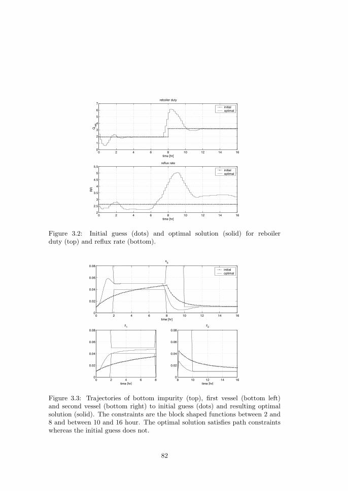
0 2 4 6 8 10 12 14 160

1

2

3

4

5

6

7reboiler duty

Qre

b

time [hr]

initialoptimal

0 2 4 6 8 10 12 14 162

2.5

3

3.5

4

4.5

5

5.5reflux rate

RR

time [hr]

initialoptimal

Figure 3.2: Initial guess (dots) and optimal solution (solid) for reboilerduty (top) and reflux rate (bottom).

0 2 4 6 8 10 12 14 160

0.02

0.04

0.06

0.08xb

time [hr]

initialoptimal

0 2 4 6 80

0.02

0.04

0.06

0.08z1

time [hr]8 10 12 14 16

0

0.02

0.04

0.06

0.08z2

time [hr]

Figure 3.3: Trajectories of bottom impurity (top), first vessel (bottom left)and second vessel (bottom right) to initial guess (dots) and resulting optimalsolution (solid). The constraints are the block shaped functions between 2 and8 and between 10 and 16 hour. The optimal solution satisfies path constraintswhereas the initial guess does not.

82

This can be written as

∆z0

∆z1

∆z2

∆z3

...∆zN

=

G00 0 0 0 . . . 0G10 G11 0 0 . . . 0G20 G21 G22 0 . . . 0G30 G31 G32 G33

.... . .

...GN0 . . . . . . . . . . . . GNN

∆u0

∆u1

∆u2

∆u3

...∆uN

, (3.14)

where Gij is the approximate ∂zi

∂uj. Note that both zi and uj are vectors.

We need to select an initial guess for the trajectory and initial condition tostart the dynamic optimization. In this case we assume the plant to be in steady-state so the initial condition is determined by the inputs at time zero. The initialguess for the optimization was determined by finding two steady-state operationconditions for the column that satisfy end product quality, not compensatingfor off spec product during transition. The reflux rate was chosen to be constantwhereas the reboiler duty was step shaped, as depicted with the line with dotsin Figure 3.2. The number of decision variables for the optimization is 192 (16hours, 2 inputs and a sample time of 10 minutes).

Path constraints t [hr] (0. . . 2) [2. . . 8) [8. . . 10) [10. . . 16]i [-] 1. . . 11 12. . . 47 48. . . 59 60. . . 96

Bottom impurity xb ≤ 0.10 0.05 0.10 0.01≥ 0.00 0.04 0.00 0.00

Impurity tank 1 z1 ≤ 0.10 0.05 - -≥ 0.00 0.04 - -

Impurity tank 2 z2 ≤ - - 0.10 0.01≥ - - 0.00 0.00

Reboiler duty Qreb ≤ 10 10 10 10≥ 0 0 0 0

Reflux ratio RR ≤ 10 10 10 10≥ 0 0 0 0

Table 3.2: Definition path constraints.

The path constraints, depicted in Figure 3.3 and shown in Table 3.2, allow fora transition of two hours after which in a period of six hours the production isquasi stationary. Stationary production is attractive from a operational pointof view but restrains flexibility and may exclude opportunities. These shouldbe carefully balanced for a reliable and economic attractive operation.

83

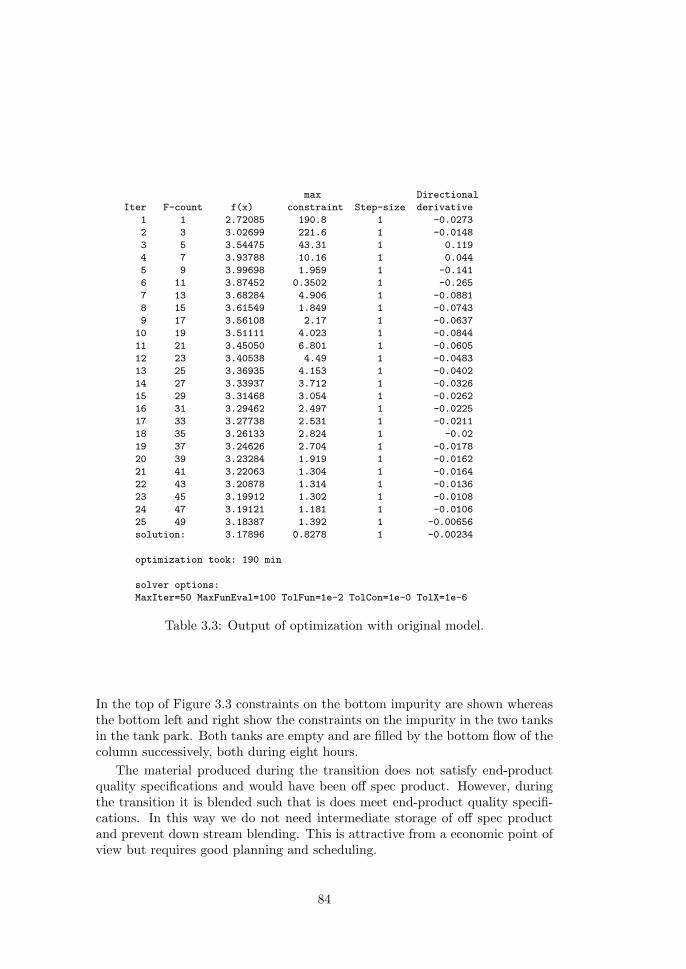
max Directional

Iter F-count f(x) constraint Step-size derivative

1 1 2.72085 190.8 1 -0.0273

2 3 3.02699 221.6 1 -0.0148

3 5 3.54475 43.31 1 0.119

4 7 3.93788 10.16 1 0.044

5 9 3.99698 1.959 1 -0.141

6 11 3.87452 0.3502 1 -0.265

7 13 3.68284 4.906 1 -0.0881

8 15 3.61549 1.849 1 -0.0743

9 17 3.56108 2.17 1 -0.0637

10 19 3.51111 4.023 1 -0.0844

11 21 3.45050 6.801 1 -0.0605

12 23 3.40538 4.49 1 -0.0483

13 25 3.36935 4.153 1 -0.0402

14 27 3.33937 3.712 1 -0.0326

15 29 3.31468 3.054 1 -0.0262

16 31 3.29462 2.497 1 -0.0225

17 33 3.27738 2.531 1 -0.0211

18 35 3.26133 2.824 1 -0.02

19 37 3.24626 2.704 1 -0.0178

20 39 3.23284 1.919 1 -0.0162

21 41 3.22063 1.304 1 -0.0164

22 43 3.20878 1.314 1 -0.0136

23 45 3.19912 1.302 1 -0.0108

24 47 3.19121 1.181 1 -0.0106

25 49 3.18387 1.392 1 -0.00656

solution: 3.17896 0.8278 1 -0.00234

optimization took: 190 min

solver options:

MaxIter=50 MaxFunEval=100 TolFun=1e-2 TolCon=1e-0 TolX=1e-6

Table 3.3: Output of optimization with original model.

In the top of Figure 3.3 constraints on the bottom impurity are shown whereasthe bottom left and right show the constraints on the impurity in the two tanksin the tank park. Both tanks are empty and are filled by the bottom flow of thecolumn successively, both during eight hours.

The material produced during the transition does not satisfy end-productquality specifications and would have been off spec product. However, duringthe transition it is blended such that is does meet end-product quality specifi-cations. In this way we do not need intermediate storage of off spec productand prevent down stream blending. This is attractive from a economic point ofview but requires good planning and scheduling.

84

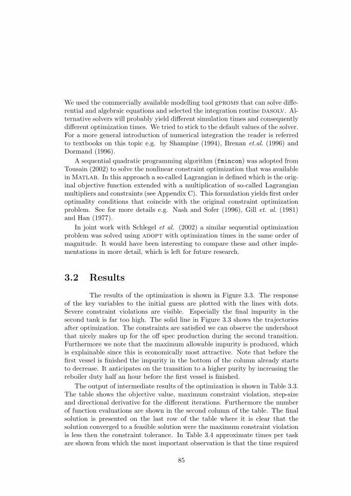
We used the commercially available modelling tool gproms that can solve diffe-rential and algebraic equations and selected the integration routine dasolv. Al-ternative solvers will probably yield different simulation times and consequentlydifferent optimization times. We tried to stick to the default values of the solver.For a more general introduction of numerical integration the reader is referredto textbooks on this topic e.g. by Shampine (1994), Brenan et.al. (1996) andDormand (1996).

A sequential quadratic programming algorithm (fmincon) was adopted fromTousain (2002) to solve the nonlinear constraint optimization that was availablein Matlab. In this approach a so-called Lagrangian is defined which is the orig-inal objective function extended with a multiplication of so-called Lagrangianmultipliers and constraints (see Appendix C). This formulation yields first orderoptimality conditions that coincide with the original constraint optimizationproblem. See for more details e.g. Nash and Sofer (1996), Gill et. al. (1981)and Han (1977).

In joint work with Schlegel et al. (2002) a similar sequential optimizationproblem was solved using adopt with optimization times in the same order ofmagnitude. It would have been interesting to compare these and other imple-mentations in more detail, which is left for future research.

3.2 Results

The results of the optimization is shown in Figure 3.3. The responseof the key variables to the initial guess are plotted with the lines with dots.Severe constraint violations are visible. Especially the final impurity in thesecond tank is far too high. The solid line in Figure 3.3 shows the trajectoriesafter optimization. The constraints are satisfied we can observe the undershootthat nicely makes up for the off spec production during the second transition.Furthermore we note that the maximum allowable impurity is produced, whichis explainable since this is economically most attractive. Note that before thefirst vessel is finished the impurity in the bottom of the column already startsto decrease. It anticipates on the transition to a higher purity by increasing thereboiler duty half an hour before the first vessel is finished.

The output of intermediate results of the optimization is shown in Table 3.3.The table shows the objective value, maximum constraint violation, step-sizeand directional derivative for the different iterations. Furthermore the numberof function evaluations are shown in the second column of the table. The finalsolution is presented on the last row of the table where it is clear that thesolution converged to a feasible solution were the maximum constraint violationis less then the constraint tolerance. In Table 3.4 approximate times per taskare shown from which the most important observation is that the time required

85

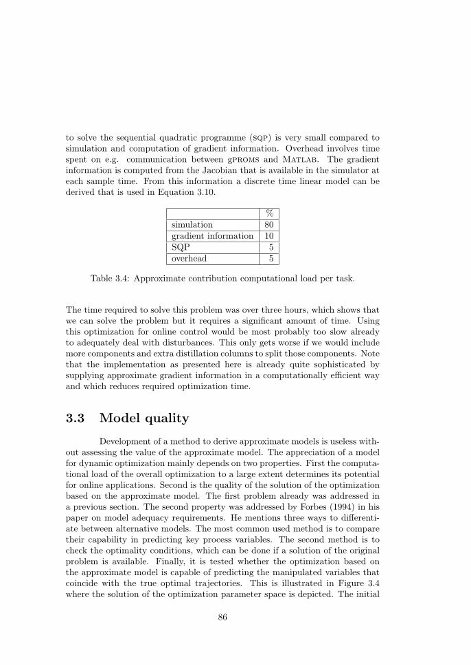
to solve the sequential quadratic programme (sqp) is very small compared tosimulation and computation of gradient information. Overhead involves timespent on e.g. communication between gproms and Matlab. The gradientinformation is computed from the Jacobian that is available in the simulator ateach sample time. From this information a discrete time linear model can bederived that is used in Equation 3.10.

%simulation 80gradient information 10SQP 5overhead 5

Table 3.4: Approximate contribution computational load per task.

The time required to solve this problem was over three hours, which shows thatwe can solve the problem but it requires a significant amount of time. Usingthis optimization for online control would be most probably too slow alreadyto adequately deal with disturbances. This only gets worse if we would includemore components and extra distillation columns to split those components. Notethat the implementation as presented here is already quite sophisticated bysupplying approximate gradient information in a computationally efficient wayand which reduces required optimization time.

3.3 Model quality

Development of a method to derive approximate models is useless with-out assessing the value of the approximate model. The appreciation of a modelfor dynamic optimization mainly depends on two properties. First the computa-tional load of the overall optimization to a large extent determines its potentialfor online applications. Second is the quality of the solution of the optimizationbased on the approximate model. The first problem already was addressed ina previous section. The second property was addressed by Forbes (1994) in hispaper on model adequacy requirements. He mentions three ways to differenti-ate between alternative models. The most common used method is to comparetheir capability in predicting key process variables. The second method is tocheck the optimality conditions, which can be done if a solution of the originalproblem is available. Finally, it is tested whether the optimization based onthe approximate model is capable of predicting the manipulated variables thatcoincide with the true optimal trajectories. This is illustrated in Figure 3.4where the solution of the optimization parameter space is depicted. The initial

86

................................................................................................................................................................................................................................................................

............................................................................................................................................................................................................................................................................................................................................................❘

....................................................................................................................................................................................................................................................................................................................................................................................................................................................................................................................................................................................

........................................

✒

...............................................................................................................................................................................................................................................................................................................................................❘

...........................................................................................................................................................

.............................................................................................................................................................

.......................

�p0

p1

p1

p2 p2

Rnp

O(M) O(M)

O(M) O(M)

Figure 3.4: Model adequacy and solution adequacy illustrated by optimizations(O) based on original model (M) and approximate model (M) mapping dif-ferent initial guesses to optimal solutions in R

np. A solution derived with anapproximate model is adequate if it satisfies optimality conditions of the opti-mization based on the original model. An approximate model is adequate if thetrue optimal solution satisfies optimality conditions of the optimization basedon the approximate model. In the graph p0 represents the initial guess that ismapped to p1 and p1 by optimizations based on the original and reduced model,respectively. Subsequently p1 and p1 are used as initial guesses for optimizationsbased on the reduced and original model, respectively. The result of these lasttwo optimizations are p2 and p2.

guess p0 can be processed by an optimization problem based on the originalmodel or based on a approximate model, O(M) or O(M), respectively. Thesetwo optimizations result in two solutions, p1 and p1 that can be used as initialguess for two alternate optimization problems where we switch models. Theseoptimizations result in two solutions p2 and p2 for the optimization based onthe original and approximate model, respectively. In case of global optimalitythe equations

p1 = p2 (3.15)p1 = p2 , (3.16)

are valid and for a good approximate model the equations

p1 ≈ p2 (3.17)p1 ≈ p2 , (3.18)

hold true.

87

An approximate model is adequate in case the distance ‖p1 − p2‖ is acceptablesmall. This implies that the predicted minimizer of the original problem is aminimizer of the optimization problem based on the approximate model.

The solution of an optimization based on an approximate model is adequatein case the distance ‖p1−p2‖ is acceptable small. This implies that the minimizerof the optimization problem with the approximate model provides a solutionthat is close to a minimizer of the original model. In case ‖p1 − p1‖ is small weexpect ‖p1−p2‖ and ‖p1− p2‖ to be small, i.e. the same local minimizers. Notethat due to local minima ‖p1− p2‖ can be large and still result in the conclusionthat solution and approximate model is accurate.

In this thesis we will assess model performance by simulation and evaluationof the key process variables and both adequacy test explained above. The opti-mization statistics will also be presented such as number of iterations, number offunction evaluations and CPU time of the optimization/simulation, to comparethe computational load of the different optimizations.

3.4 Discussion

In this chapter we showed a sensible dynamic optimization problem fora typical chemical process. Although great effort was put into this formulationone could think of arguments that would result in a different formulation of theoptimization problem.

An interesting extension of this problem would have been for example to addthe fresh feed to the set of optimization variables and add constraints on thelevels in the tank park. Furthermore, the time interval allowed for transitioncould be enlarged providing more freedom and possibly more opportunities foreconomic improvement. These scenarios were regarded as very interesting butdid not add extra value to purpose of this example namely the study of differentmodel reduction techniques for dynamic optimization. Nevertheless this caserepresents a large class of optimization problems in the process industry.

The optimization was successfully implemented and provided optimal trajec-tories that would be acceptable for real implementation. For off line trajectoryoptimization we could stop here but for online optimization a sample time largerthan tree hours is not acceptable. Computational load is the main hurdle toovercome going from off line to an online implementation that is fast enough toadequately respond to disturbances.

We motivated and provided detailed information on the implementationof the optimization problem. This is necessary to interpret the results sinceseemingly unimportant details can have a decisive impact. Although we wouldexpect similar optimal trajectories for a simultaneous optimization approach wedid not put effort in comparing these two approaches.

88

Chapter 4

Physics-based modelreduction

In this chapter model reduction based on physics (remodelling) is discussed.We will start to present the rigorous model for a reaction separation processfollowed by the physics-based reduced model. Modelling assumptions are thekey for this reduction. This approach is mainly inspired on the question whatthe added value is of detailed modelling for dynamic optimization. Simplifiedmodels became outdated because for simulation purposes it was not a problem todevelop and use more detailed models. Dynamic optimization is computationallymore demanding than simulation and therefore the idea arose to fall back tosimple models. The quality of the reduced model is assessed in the last sectionby execution of a dynamic optimization based on the reduced model.

4.1 Rigorous model

The process consists of a reactor and distillation column as depicted inthe flow sheet in Figure 3.1. The reactor is fed by a fresh feed and the recyclestream from the top of the distillation. The outlet of the reactor is connectedto the feed of the column. First we will describe the very simple reactor modelfollowed by the column model, which is far more complex and therefore a bettercandidate for remodelling. The detailed column model is a standard modelwith component balances and an energy balance. The physical properties modelused to derive gas and liquid fugacity, enthalpy and density is based on a cubicequation of state as described in Reid (1987). The simplified model is based ona constant molar overflow model and constant relative volatility as described in

89

Skogestad (1997). This last model was slightly modified by making the relativevolatility a dependent of composition.

Reactor model

The reactor is modelled as a continuously stirred tank reactor (cstr). We as-sume the content to be ideally mixed, which implies no temperature and noconcentration gradients within the reactor occur. In the reactor a first orderexothermic irreversible reaction A → B takes place without side reactions, soonly two species are modelled. The reaction rate depends on concentration CA

and temperature described by an Arrhenius equation.

Total molar balancedN

dt= F0 +D − F , (4.1)

where N is the total molar holdup in the reactor, F0 is the fresh feed, D is therecycle flow from the top of the distillation column and F is the product flowout of the reactor. All flows are total molar flows of the both reactant A andproduct B. The outgoing flow F is controlled by a level controller. The freshfeed F0 is assumed to be determined by the upstream process. The distillateflow D is controlled by the level controller on the condenser.

Component mass balance

ρmdNz

dt= ρmF0z0 + ρmDxd − ρmFz − k0CAV e

−EaRT , (4.2)

where ρm is the molar density of both the reactant A and product B, z is themolar fraction of A in the reactor, xd and z are molar fractions of A in recycleand fresh feed flow, k0 and Ea are reaction rate and activation constants, respec-tively, and R is the relative gas constant. CA and T are the molar concentrationand temperature in the reactor and V is the volume in the reactor of reactantA and product B together. The component mass balance can be rearrangedby substitution of the equalities dNz

dt = N dzdt + z dN

dt , CAV = Nz and the totalmolar balance:

Component balance rearranged

dz

dt=

F0

N(z0 − z) +

D

N(xd − z)− k0

ρme

−EaRT z . (4.3)

Energy balance

ρmcpdNT

dt= ρmcp(F0T0 +DTd − FT )−Q+ k0CAV e

−EaRT ∆H , (4.4)

90

where cp is the specific heat and assumed to be independent of temperature andindependent of composition, T0, Td and T are temperatures of fresh feed, dis-tillate flow and temperature in the reactor, respectively. Q is the heat removedfrom the reactor by cooling and ∆H is the reaction heat constant.

Heat removal

dρccpcVcTcdt

= ρccpcΦc(Tci − Tc) +Q (4.5)

Q = αcAc(T − Tc) . (4.6)

where ρc, cpc, Vc and Tc are density, specific heat, volume and temperature ofthe cooler, respectively. Φc is the coolant flow rate and Tci is the temperatureof the coolant at the inlet of the heat exchanger. Ac and αc are the total heattransfer coefficient and the total area of heat transfer between coolant and re-actor content. We assume the dynamics to be very fast and the coolant in theheat exchanger to be ideally mixed. It is clear that by manipulating the coolantflow rate, Φc, we can control the coolant temperature Tc. Tc determines with Tthe driving force for the heat removal. A controller that measures the tempera-ture in the reactor and actuates on the coolant flow rate can in this way controlthe heat removal and therefore the reactor temperature. If the temperaturecontroller is well tuned and the heat exchanger is well designed we can assumethat we directly manipulate the heat removal. In the plant model that is usedin this thesis we assume that the heat exchanger is well designed. Therefore theequations describing the heat exchanger are not included and the temperaturecontroller directly controls the heat removal.

The energy balance can be rearranged by substitution of the equalities dNTdt =

N dTdt + T dN

dt , CAV = Nz and the total molar balance.

Energy balance rearranged

dT

dt=

F0

N(T0 − T ) +

D

N(Td − T )− Q

N

1ρmcp

+ (4.7)

1ρmcp

k0e−EaRT z∆H .

The reactor model is very simple, however, without tight temperature controleven this very simple model can exhibit limit cycling behavior.

We could add two modelling assumptions that simplify the reactor modeleven further. We could assume the temperature and level to be constant. Thisassumption can be motivated by the assumption that we are able to controlthese variables very fast. The controlled variables are now considered to be

91

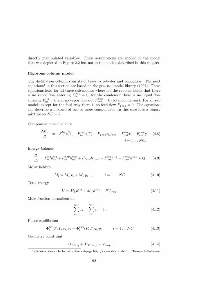
directly manipulated variables. These assumptions are applied in the modelthat was depicted in Figure 2.2 but not in the models described in this chapter.

Rigorous column model

The distillation column consists of trays, a reboiler and condensor. The nextequations1 in this section are based on the gproms model library (1997). Theseequations hold for all three sub-models where for the reboiler holds that thereis no vapor flow entering F vap

in = 0, for the condensor there is no liquid flowentering F liq

in = 0 and no vapor flow out F vapout = 0 (total condensor). For all sub

models except for the feed tray there is no feed flow Ffeed = 0. The equationscan describe a mixture of two or more components. In this case it is a binarymixture so NC = 2.

Component molar balance

dMi

dt= F liq

in zliqi,in + F vapin zvapi,in + Ffeedzi,feed − F liq

outxi − F vapout yi (4.8)

i = 1 . . . NC.

Energy balance

dU

dt= F liq

in hliqin + F vapin hvapin + Ffeedhfeed − F liq

outhliq − F vap

out hvap +Q . (4.9)

Molar holdup

Mi =MLxi +MV yi , i = 1 . . . NC. (4.10)

Total energy

U =MLhliq +MV hvap − PVtray . (4.11)

Mole fraction normalization

NC∑i=1

xi =NC∑i=1

yi = 1 . (4.12)

Phase equilibrium

Φliqi (P, T, xi)xi = Φ

vapi (P, T, yi)yi i = 1 . . . NC. (4.13)

Geometry constraint

MLvliq +MV vvap = Vtray . (4.14)1gproms code can be found on the webpage http://www.dcsc.tudelft.nl/Research/Software.

92

Level of clear liquid

Lliq =MLvliqAp

. (4.15)

Furthermore we used a physical property model based on a cubic equation ofstate from which the properties of the liquid phase as well as the properties ofthe vapor phase can be computed.

The Soave equation of state

Z3 − Z2 + (A−B −B2)Z −AB = 0 . (4.16)

where

A =aP

R2T 2(4.17)

B =bP

RT. (4.18)

The values of a and b can be deduced from the critical of the pure componentsproperties and acentric factor and mixing rules

ai = 0.42748R2T 2

c,i

Pc,i

(1 + fw,i(1−

√T

Tc,i)

)2

(4.19)

fw,i = 0.48 + 1.574wi − 0.17w2i (4.20)

bi = 0.08664RTc,iPc,i

. (4.21)

The values of a and b for mixtures are given by the following mixing rules

a =

(NC∑i=1

zi√ai

)2

(4.22)

b =NC∑i=1

zibi . (4.23)

where zi is the molar fraction in the mixture.

The cubic equation is solved, which yields three real roots

Zl ≤ Zj ≤ Zv . (4.24)

93

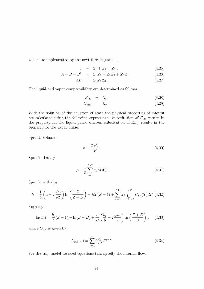
which are implemented by the next three equations

1 = Z1 + Z2 + Z3 , (4.25)A−B −B2 = Z1Z2 + Z2Z3 + Z3Z1 , (4.26)

AB = Z1Z2Z3 . (4.27)

The liquid and vapor compressibility are determined as follows

Zliq = Zl , (4.28)Zvap = Zv . (4.29)

With the solution of the equation of state the physical properties of interestare calculated using the following expressions. Substitution of Zliq results inthe property for the liquid phase whereas substitution of Zvap results in theproperty for the vapor phase.

Specific volume

v =ZRT

P. (4.30)

Specific density

ρ =1v

NC∑i=1

xiMWi . (4.31)

Specific enthalpy

h =1b

(a− T

∂a

∂T

)ln(

Z

Z +B

)+RT (Z − 1) +

NC∑i=1

xi

∫ T

Tref

Cp,i(T )dT. (4.32)

Fugacity

ln(Φi) =bib(Z − 1)− ln(Z −B) +

A

B

(bib− 2

√aia

)ln(Z +B

Z

), (4.33)

where Cp,i is given by

Cp,i(T ) =4∑

j=1

C(j)p,i T

j−1 . (4.34)

For the tray model we need equations that specify the internal flows.

94

Overflow over weir

F liqoutvliq = 1.84Lw

(Lliq − βhw

β

) 32

. (4.35)

Pressure drop over the plate

F vapin =

Ah

vvap

√P vapin − P − ρliqgLliq

αρvap. (4.36)

Adiabatic operation of a tray

Q = 0 . (4.37)

For reboiler and condensor Q in not equal to zero because of the heat input andheat removal, respectively. Not all streams are present in all sub-models. Onlyat the feed tray the feed enters the column so for all other trays the feed becomeszero. Furthermore, in the reboiler there does not enter a vapor stream whereasin the condensor there does not exit any vapor stream (total condensor). Theseequations were put together in a rigorous model for the reaction separationprocess.

4.2 Physics-based reduced model

From literature we know that a simple way of modelling a distillationcolumn is to assume constant molar holdup, constant molar overflow and con-stant relative volatility (see e.g. Skogestad, 1997). Such a model is probablytoo simple for our case but will provide the starting point for our physicallyreduced model2.

Component molar balance

dMi

dt= F liq

in zliqi,in + F vapin zvapi,in + Ffeedzi,feed − F liq

outxi − F vapout yi (4.38)

i = 1 . . . NC.

Molar holdup is in the liquid phase

Mi =MLxi +MV yi ≈ MLxi , i = 1 . . . NC. (4.39)

Mole fraction normalizationNC∑i=1

xi =NC∑i=1

yi = 1 . (4.40)

2gproms code can be found on the webpage http://www.dcsc.tudelft.nl/Research/Software.

95

Phase equilibrium by constant relative volatility

yi =αi∑NC

i=1 αixixi , i = 1 . . . NC. (4.41)

Linearized liquid dynamics

F liqout = F liq

out

∗+

ML −M∗L

τ. (4.42)

Constant vapor stream

F vapout = F vap

in . (4.43)

We will now go the details of the different assumptions that yield the reducedmodel. An important assumption needed for the physical based model reductionis that the pressure in the column is controlled at a constant set point. Thisseems somewhat restrictive but in practice the pressure set point is not the mainhandle for control of a distillation column. If the pressure drop over the columnis negligible compared to the absolute pressure we can assume the pressure to beconstant if we consider physical properties. The assumption of constant pressurein the column with respect to the internal vapor flux is not valid since only apressure difference can enforce a flow. Still we need to determine the internalvapor flow.

Constant molar vapor stream

Start with a steady-state assumption for the molar holdup and energy balance

0 = F liqin − F liq

out + F vapin − F vap

out (4.44)

0 = F liqin hliqin − F liq

outhliq + F vap

in hvapin − F vapout h

vap . (4.45)

Elimination of F liqin yields

0 = F liqout(h

liqin − hliq)− F vap

in (hliqin − hvapin ) + F vapout (h

liqin − hvap) . (4.46)

The specific enthalpy of the liquid phase is much larger than the specific enthalpyof the vapor phase. This combined with the small differences in specific enthalpyof neighboring trays justifies the assumption that

hevap = hliqin − hvapin ≈ hliqin − hvap . (4.47)

Substitution yields

0 = F liqout(h

liqin − hliq)− (F vap

in − F vapout )h

evap . (4.48)

96

Rearranging this equation yields

hliqin − hliq

hevap=

F vapin − F vap

out

F liqout

. (4.49)

With the same argument that the differences of specific enthalpy of two neigh-boring trays is small relative to the heat of evaporation combined with vaporstreams that are in the same order of magnitude of the liquid streams, the dif-ference in vapor streams must be approximately zero. Therefore we can assume

F vapout = F vap

in . (4.50)

Linearized hydrodynamics

In the rigorous model the liquid flow over the weir is described by

F liqout =

1.84vliq

(Lliq − βhw

β

) 32

. (4.51)

This equation can be linearized in L∗liq

F liqout = F ∗

liq +32

(1.84v∗liq

)(L∗liq − βhw

β

) 12 1β∆Lliq = F ∗

liq +∆Lliq

τ∗h, (4.52)

where τ∗h is the hydraulic time constant in that operating point and ∆Lliq =Lliq −L∗

liq. This approach was adopted from Skogestad (1997). The value of τ∗hcan be directly computed from the parameters and steady state values of therigorous model. In the simplified model we need to rewrite the equation as afunction of the molar liquid holdup. This is done with Mliq vliq = LliqAp

F liqout = F ∗

liq +∆Mliq v

∗liq

τ∗hAp, (4.53)

with ∆Mliq =Mliq −M∗liq.

We can reduce the liquid hydrodynamics even further by assuming thatthe liquid holdup on a tray is constant. This is equal to the assumption thatF liqin = F liq

out. This assumption was only applied in the model used in Chapter 2.

Boilup rate and reboiler duty

Furthermore we need to add a new equation that relates the heat input to amolar flow since the energy balance was eliminated. Again it starts with thequasi steady-state assumption of mass and heat balance

0 = F liqin + F liq

out + F vapout (4.54)

0 = F liqin hliqin + F liq

outhliq + F vap

out hvap +Qreb . (4.55)

97

Elimination of F liqin yields

0 = F liqout(h

liqin − hliq) + F vap

out (hliqin − hvap) +Qreb . (4.56)

And with the argument that the difference in specific enthalpy between liquidand vapor is much larger than the difference in specific liquid enthalpy of twoneighboring trays, 0 ≈ hliqin − hliq hliqin − hvap ≈ hevap, the equation can beapproximated by

0 ≈ F vapout (h

liqin − hvap) +Qreb (4.57)

≈ F vapout h

evap +Qreb . (4.58)

Despite the fact that hevap(P, T, x) is a function of pressure, temperature andcomposition, we will assume it to be constant since the variations are in generalquite small.

Constant relative volatility

The vapor-liquid equilibrium in the simplified model is computed by the con-stant relative volatility equation

yi =αi∑NC

j=1 αjxjxi . (4.59)

We can observe that the equation is very simple compared to the cubic equationof state approach. In particular, the equations can be solved explicitly if wechoose x as a state variable.

Underlying assumption for this simplification is that the pressure does notplay a role for the vapor-liquid equilibrium, which in general is certainly nottrue. In practice a column is operated at a controlled pressure and therefore wecan neglect pressure effects on the vapor-liquid equilibrium.

The constant relative volatility was derived in order to remove the tempera-ture effects on the vapor liquid equilibrium and therefore is implicitly accountedfor in the constant relative volatility approach. Still we need to check whetherthe relative volatility is indeed constant. This can be checked by computing therelative volatility in the original model.

It appears that in this case the relative volatility is not constant. Nextstep is to find an explicit relation that describes the relation of the observedrelative volatility. This is where the engineering comes in and can hardly beautomated. After some trial and error we came up with the following extensionof the relative volatility

αi(xi) = θ1,i + θ2,ixi . (4.60)

98

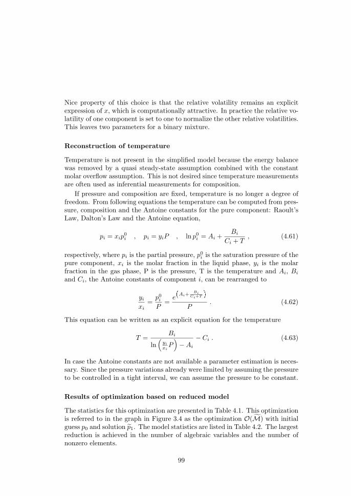
Nice property of this choice is that the relative volatility remains an explicitexpression of x, which is computationally attractive. In practice the relative vo-latility of one component is set to one to normalize the other relative volatilities.This leaves two parameters for a binary mixture.

Reconstruction of temperature

Temperature is not present in the simplified model because the energy balancewas removed by a quasi steady-state assumption combined with the constantmolar overflow assumption. This is not desired since temperature measurementsare often used as inferential measurements for composition.

If pressure and composition are fixed, temperature is no longer a degree offreedom. From following equations the temperature can be computed from pres-sure, composition and the Antoine constants for the pure component: Raoult’sLaw, Dalton’s Law and the Antoine equation,

pi = xip0i , pi = yiP , ln p0

i = Ai +Bi

Ci + T, (4.61)

respectively, where pi is the partial pressure, p0i is the saturation pressure of the

pure component, xi is the molar fraction in the liquid phase, yi is the molarfraction in the gas phase, P is the pressure, T is the temperature and Ai, Bi

and Ci, the Antoine constants of component i, can be rearranged to

yixi=

p0i

P=

e

�Ai+

BiCi+T

�

P. (4.62)

This equation can be written as an explicit equation for the temperature

T =Bi

ln(yi

xiP)−Ai

− Ci . (4.63)

In case the Antoine constants are not available a parameter estimation is neces-sary. Since the pressure variations already were limited by assuming the pressureto be controlled in a tight interval, we can assume the pressure to be constant.

Results of optimization based on reduced model

The statistics for this optimization are presented in Table 4.1. This optimizationis referred to in the graph in Figure 3.4 as the optimization O(M) with initialguess p0 and solution p1. The model statistics are listed in Table 4.2. The largestreduction is achieved in the number of algebraic variables and the number ofnonzero elements.

99

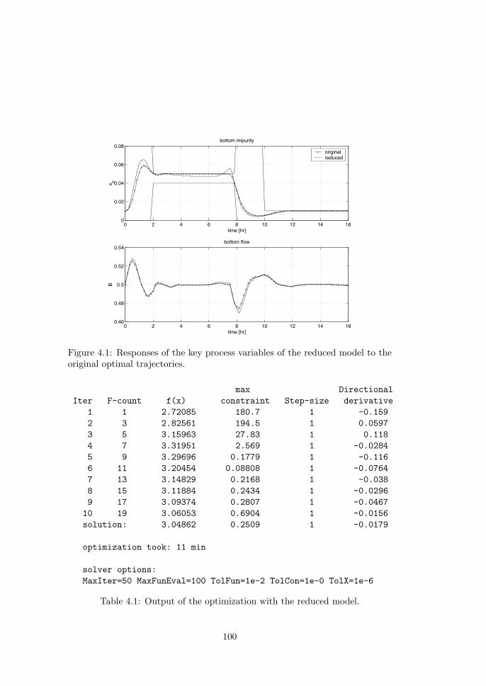
0 2 4 6 8 10 12 14 160

0.02

0.04

0.06

0.08bottom impurity

x b

time [hr]

originalreduced

0 2 4 6 8 10 12 14 160.46

0.48

0.5

0.52

0.54bottom flow

B

time [hr]

Figure 4.1: Responses of the key process variables of the reduced model to theoriginal optimal trajectories.

max DirectionalIter F-count f(x) constraint Step-size derivative

1 1 2.72085 180.7 1 -0.1592 3 2.82561 194.5 1 0.05973 5 3.15963 27.83 1 0.1184 7 3.31951 2.569 1 -0.02845 9 3.29696 0.1779 1 -0.1166 11 3.20454 0.08808 1 -0.07647 13 3.14829 0.2168 1 -0.0388 15 3.11884 0.2434 1 -0.02969 17 3.09374 0.2807 1 -0.0467

10 19 3.06053 0.6904 1 -0.0156solution: 3.04862 0.2509 1 -0.0179

optimization took: 11 min

solver options:MaxIter=50 MaxFunEval=100 TolFun=1e-2 TolCon=1e-0 TolX=1e-6

Table 4.1: Output of the optimization with the reduced model.

100

Compared to the optimization with the original model, see Table 3.3, the num-ber of iterations is reduced by a factor of more than two. This does not explainthe factor seventeen in reduction of the overall optimization time. Simulationswith the reduced model are less computational demanding (approximately afactor seven) and this is the second explanation for the tremendous reduction.Note that the only difference between the two optimizations is the function eva-luation and the gradient information since these are based on different models.

model: nx ny na nnz

original 75 1912 24 7237reduced 54 211 24 859ratio 1.4 9.1 1.0 8.4

Table 4.2: Properties original and reduced model with nx, ny and na the numberof differential, algebraic and assigned (fixed) variables, respectively. nnz is thenumber of nonzero elements in the Jacobian.

Furthermore, note that reduction in simulation times by a factor of seven canbe associated best with the reduction of the number of nonzero elements, whichis a factor of eight approximately. This association is closer than the reductionratio of differential equations or total number of equations.

The quality of model and the solution of this dynamic optimization are topicof the next section.

4.3 Model quality

As presented in Chapter 3 we can assess model quality in three differentmanners. These three will be applied in this section. First we will present theevaluation by simulation. Secondly, we assess model adequacy by verifyingoptimality conditions of the optimization based on the reduced model with thesolution of the original optimization problem. This optimization is referred toin the graph in Figure 3.4 as the optimization O(M) with initial guess p1 andsolution p2. Finally, we present the reversed check for optimality conditionsreferred to as the optimization O(M) with initial guess p1 and solution p2.In that case the optimality conditions for the optimization problem with theoriginal model for the approximate solution are checked.

101

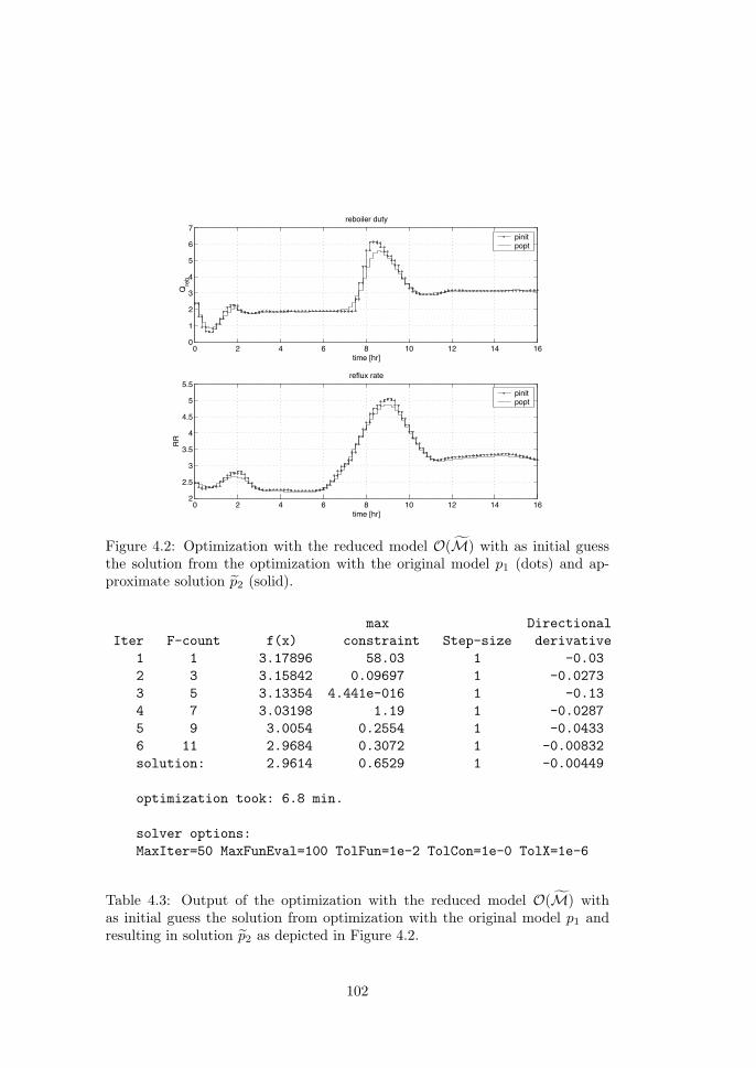
0 2 4 6 8 10 12 14 160

1

2

3

4

5

6

7reboiler duty

Qre

b

time [hr]

pinitpopt

0 2 4 6 8 10 12 14 162

2.5

3

3.5

4

4.5

5

5.5reflux rate

RR

time [hr]

pinitpopt

Figure 4.2: Optimization with the reduced model O(M) with as initial guessthe solution from the optimization with the original model p1 (dots) and ap-proximate solution p2 (solid).

max DirectionalIter F-count f(x) constraint Step-size derivative

1 1 3.17896 58.03 1 -0.032 3 3.15842 0.09697 1 -0.02733 5 3.13354 4.441e-016 1 -0.134 7 3.03198 1.19 1 -0.02875 9 3.0054 0.2554 1 -0.04336 11 2.9684 0.3072 1 -0.00832solution: 2.9614 0.6529 1 -0.00449

optimization took: 6.8 min.

solver options:MaxIter=50 MaxFunEval=100 TolFun=1e-2 TolCon=1e-0 TolX=1e-6

Table 4.3: Output of the optimization with the reduced model O(M) withas initial guess the solution from optimization with the original model p1 andresulting in solution p2 as depicted in Figure 4.2.

102

Evaluation by simulation

A simple check of model quality is to do two simulations, first with the originaland repeat the simulation with the reduced model. Comparison of the keyprocess variables gives a fist impression of model quality. For the test of thereduced model as discussed in this chapter we used the optimal trajectoriescomputed by the optimization based on the original model. These trajectorieswhere applied to the reduced model and Figure 4.1 shows the responses ofbottom impurity and bottom flow. These process variables are considered to bethe key process variables.

We see that constraints for the bottom impurity are not satisfied at alltimes but the constraint violation is minimal. These minor differences can beascribed to small differences in internal flows related to the constant molar vaporflow assumption. A separate check on the relative volatility showed that theapproximation was nearly perfect for the range of operation that was consideredhere.

Differences in bottom flow rate are very small. In steady-state these cannotdiffer because that would imply a violation of the conservation laws since it isthe only way out of the process.

Model adequacy

The second approach to assess model quality is to check the optimality condi-tions of the optimization based on the reduced model with the true optimum.Or stated differently, check whether or not the true optimum is also an optimumfor the optimization based on the reduced model.

Results of these tests are presented in Figure 4.2. Some minor changes can benoted mainly due to the constraint violation that occurs with the original guess.This can be verified in the Table 4.3 that confirms the constraint violation at thefirst iteration. Note that the responses of the key process variables to the initialguess coincides with the responses used for the comparison based on simulationand therefore equal to the responses depicted in Figure 4.1. Remarkable is thetime still needed to converge (Table 4.3) compared to the result as presented inTable 4.1 with the step shaped initial guess. Despite the initial guess is quitegood the warm started optimization is less than two times faster compared tothe optimization with a cold start.

Although this is a sensible approach to assess the model quality for dynamicoptimization, in practice we would like to do optimizations based on the re-duced model and assess the quality of those solutions. This is precisely what isdiscussed next.

103

0 2 4 6 8 10 12 14 160

1

2

3

4

5

6

7reboiler duty

Qre

b

time [hr]

pinitpopt

0 2 4 6 8 10 12 14 162

2.5

3

3.5

4

4.5reflux rate

RR

time [hr]

pinitpopt

Figure 4.3: Optimization with the original model O(M) with as initial guessthe approximate solution from optimization with the reduced model p1 (dots)and resulting solution p2 (solid).

max DirectionalIter F-count f(x) constraint Step-size derivative

1 1 3.04862 73.07 1 0.1842 3 3.29795 24.13 1 0.07673 5 3.39243 10.71 1 -0.02154 7 3.37446 0.4812 1 -0.06555 9 3.32522 0.07207 1 -0.02216 11 3.30531 0.3974 1 -0.0149solution: 3.29149 0.02154 1 -0.00599

optimization took: 46.8 min.

solver options:MaxIter=50 MaxFunEval=100 TolFun=1e-2 TolCon=1e-0 TolX=1e-6

Table 4.4: Output of the optimization with the original model O(M) withas initial guess the approximate solution from optimization with the reducedmodel p1 and resulting in solution p2 as depicted in Figure 4.3.

104

Solution adequacy

The capability of a reduced or approximate models to predict optimal solutionsthat are acceptable close to the true process optimum is crucial. This capabilityis tested by redoing the optimization based on the original model with theapproximate solution as initial guess derived with the reduced model.

The result of this test is depicted in Figure 4.3 where the input trajectoriesof the reboiler duty and reflux rate are shown. Again we only observe minordifferences between initial guess and converged solution. The intermediate sta-tistics are gathered in Table 4.4, which shows an initial constraint violation thatis satisfied at cost of an increased objective value.

Note that the optimal solutions represent local minima. This is clearly visibleif we compare the reflux rate in Figures 4.2 and 4.3. This may be caused bya lack of sensitivity for this input channel. The shape of the optimal inputtrajectories of the boilup rate are striking similar, which pleas for the followedapproach.

From a computational point of view we already concluded that is was veryattractive to use the reduced model, reducing computation time with a factorof seventeen. If we use the reduced model only for computation of an initialguess as a first step, we still reduce the computational effort by more than afactor three. The local minimum of the original optimization problem is slightlybetter than a two-step approach. This emphasizes that we indeed found a localminimizer.

A last comment is that coincidentally the same number of iteration is neededfor convergence as in the previous test.

4.4 Discussion

In this chapter the added value of a physically reduced model becameevident for this dynamic optimization problem. A significant reduction in com-putational time was achieved using the reduced model. Even when this solutionwas used as an initial guess for the optimization with the detailed model theoverall time for optimization is shorter3.

In practice, one could argue what the added value is of the use of the detailedmodel since the quality of the reduced model is already quite high. Especiallyconsidering that there will also be mismatch between the detailed model andthe real plant. Furthermore the presence of disturbances will require a feedbackmechanism. Since the performance of a feedback controller is limited by thesample rate a controller based on a detailed model with low sample rate can be

3In a closed loop implementation the converged solution of the previous cycle could beused to construct an good initial guess.

105

outperformed by a controller based on a simple less accurate model with a highsample rate.

The approach to derive the simplified model can be generalized to modelsthat describe physical properties based on detailed physical property models e.g.based on a Soave equation of state. These detailed physical property modelshave a large validity range that is not exploited within the dynamic optimization.This allows for simplification by using simplified models available from literatureIn this thesis the simplified distillation column from Skogestad (1997) was used.This model was extended with equations that reconstruct variables that arepresent in the detailed model but not available in the simplified model.

Key to the success of this approach is that the simplified model has similarproperties as the detailed model. The simplified model has a similar sparsitystructure and nonlinearity but with less differential and algebraic equations.Inevitably will an optimization based on such a model be computationally lessdemanding. It requires detailed process knowledge to distinguish between rele-vant phenomena and less important details to come to a right tradeoff.

Should this dynamic optimization run online we saw that a warm startedoptimization with the reduced model is seven times faster than the optimizationwith the original. A closed loop evaluation with disturbances is not performedin this thesis but a controller based on the reduced model and a sampling rate often minutes would most likely outperform the controller based on the rigorousmodel and sampling rate of almost one hour. How much better the controllerwould be mainly depends on the character of the disturbances.

106

Chapter 5

Model order reduction byprojection

In this chapter the possibilities of model order reduction by projection for dy-namic optimization are explored. The focus in this chapter will be on the modelquality whereas the techniques to derive the projection have been discussed Chap-ter 2 of this thesis. Proper Orthogonal Decomposition and a Gramian based re-duction are applied to the physics-based reduced model as presented in Chapter 4and assessed within a dynamic optimization problem as outlined in Chapter 3.

5.1 Introduction

In Chapter 2 model order reduction by projection has been discussed.Because of its success in reducing model order significantly while keeping theapproximation error small it was selected as a promising model reduction tech-nique for dynamic optimization. Two different approaches to derive a suitableprojection are selected. The first approach is based on a proper orthogonaldecomposition of data generated by simulation of the optimal trajectory resul-ting from the optimization as defined in Chapter 3. The second approach isa balanced reduction based on averaging controllability Gramians and avera-ging observability Gramians derived along the same optimal trajectory (thatwas used for proper orthogonal decomposition) via linearization and Lyapunovequations.

In this chapter we will assess those two different projection techniques forboth truncation and residualization and for all reduced model orders. As areference model we use the physics-based reduced model as presented in Chap-ter 4, which has forty seven differential equations. With two different projection

107

techniques and both truncation and residualization we have almost two hundredreduced-order models that will be assessed in this chapter.

The motivation for assessing all model orders is that in literature no leadsare available how to find the optimal order for the projected model. One expectsa gradual increase of the simulation approximation error when increasing thelevel of reduction. At the same time one expects that increasing the level ofreduction results in a gradual decrease of computational load of simulation. Forthe sequential approach implementation of dynamic optimization, a reductionof computational load of the simulation directly results in a reduction in timerequired for one iteration. Model reduction by projection is therefore expectedto reduce the overall computational effort assuming that the number of iterationsremains approximately the same for the optimization.

Difference between model reduction by truncation and by residualizationis that in case of residualization the steady state approximation error is zerowhereas for truncation in general this is not the case. Note that model reductionby singular perturbation is also a reduction by residualization. However, modelreduction by singular perturbation is based on a modal analysis whereas properorthogonal decomposition and Gramian based reduction are based on an energymeasure from input to state or output, respectively. For dynamic optimizationa zero steady-state approximation error is a favorable property because the tailof the solution is dominated by low frequent dynamics and approach a steady-state.

When comparing proper orthogonal decomposition with Gramian based re-duction both methods have strong and weak points. Strong point for properorthogonal decomposition is that the reduction is based on a trajectory, whichcan be an optimal trajectory based on the full-order model. The reduction istailored for this specific trajectory and requires a conscious choice of input tra-jectories used for model reduction. Recall however that the result also dependson scaling of the different state variables. Gramian based reduction does not de-pend on the scaling of states and really takes the input to output behavior intoaccount. On the other hand the projection matrix required for a Gramian-basedprojection can be close to singular whereas the projection matrix for proper or-thogonal decomposition is orthogonal. It is hard to predict what method shouldbe preferred.

It is not possible to give an analytical answer to the question which modelprojection approach provides the best results in terms of quality and reduction ofcomputational load. Therefore in this chapter these different projection methodsare assessed experimentally within an optimization environment. Based on theresults we can answer the question whether it is possible to successfully applydifferent projected models within dynamic optimization. This will be done basedon performance indicators that are outlined next.

108

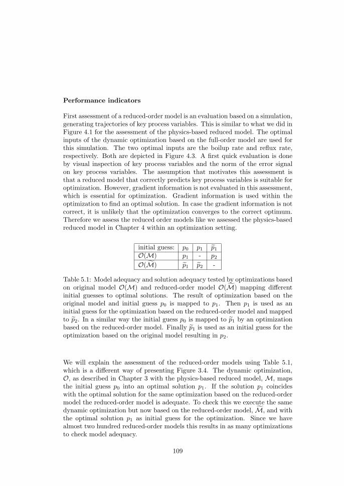
Performance indicators

First assessment of a reduced-order model is an evaluation based on a simulation,generating trajectories of key process variables. This is similar to what we did inFigure 4.1 for the assessment of the physics-based reduced model. The optimalinputs of the dynamic optimization based on the full-order model are used forthis simulation. The two optimal inputs are the boilup rate and reflux rate,respectively. Both are depicted in Figure 4.3. A first quick evaluation is doneby visual inspection of key process variables and the norm of the error signalon key process variables. The assumption that motivates this assessment isthat a reduced model that correctly predicts key process variables is suitable foroptimization. However, gradient information is not evaluated in this assessment,which is essential for optimization. Gradient information is used within theoptimization to find an optimal solution. In case the gradient information is notcorrect, it is unlikely that the optimization converges to the correct optimum.Therefore we assess the reduced order models like we assessed the physics-basedreduced model in Chapter 4 within an optimization setting.

initial guess: p0 p1 p1

O(M) p1 - p2

O(M) p1 p2 -

Table 5.1: Model adequacy and solution adequacy tested by optimizations basedon original model O(M) and reduced-order model O(M) mapping differentinitial guesses to optimal solutions. The result of optimization based on theoriginal model and initial guess p0 is mapped to p1. Then p1 is used as aninitial guess for the optimization based on the reduced-order model and mappedto p2. In a similar way the initial guess p0 is mapped to p1 by an optimizationbased on the reduced-order model. Finally p1 is used as an initial guess for theoptimization based on the original model resulting in p2.

We will explain the assessment of the reduced-order models using Table 5.1,which is a different way of presenting Figure 3.4. The dynamic optimization,O, as described in Chapter 3 with the physics-based reduced model, M, mapsthe initial guess p0 into an optimal solution p1. If the solution p1 coincideswith the optimal solution for the same optimization based on the reduced-ordermodel the reduced-order model is adequate. To check this we execute the samedynamic optimization but now based on the reduced-order model, M, and withthe optimal solution p1 as initial guess for the optimization. Since we havealmost two hundred reduced-order models this results in as many optimizationsto check model adequacy.

109

Conversely, we can execute a dynamic optimization based on the reduced-ordermodel with p0 as initial guess for the optimization. This results in an optimalsolution p1 for each reduced-order model. The quality of this solution canbe checked in a similar way as we checked the quality of the reduced-ordermodels. We repeat the dynamic optimization based on the full-order modelM and use p1 as the initial guess for the optimization. If the solution basedon the reduced-order model coincides with the optimal solution for the full-order model the solution is adequate. Again this results in almost two hundredoptimizations. Before executing these optimizations a first quick evaluation ofthe optimal solution p1 is done by visual inspection. This is done by comparingthese solutions to the optimal solution p1 based on the full-order model.

Besides the model quality we are interested in the computational load ofthe dynamic optimization based on the reduced-order models. The results oncomputational load of the dynamic optimization and the number of iterationsto reach convergence are defined as performance indicators. Note that for theevaluation of the reduced models we use the same initial guess, p0, for the opti-mization. First we will continue with the properties of the nonlinear models andthe implementation of projection of a set of differential and algebraic equations.Then we will present the results of all optimizations as discussed in this sectionto assess reduced-order model quality.

5.2 Projection of nonlinear models

Model properties

The class of models that are considered in this thesis can be described by a setof differential and algebraic equations (dae) of at most index one (Brenan etal., 1996),

0 = F (x, x, y, u) , (5.1)

where x ∈ Rnx are defined as state variables, y ∈ R

ny are defined as algebraicvariables, u ∈ R

nu are defined as input variables and t ∈ R is defined as thevariable time. Here nx is referred to as the order of the model.We will confine to models defined by a set of explicit differential algebraic equa-tions

x = f(x, y, u)0 = g(x, y, u) , (5.2)

where f ∈ Rnx and g ∈ R

ny . This can be written in the general format as

0 = F (x, x, y, u) =[

−x+ f(x, y, u)g(x, y, u)

]. (5.3)

110

This shows precisely the structure that is imposed on the models that we con-sider in this chapter.

A special case occurs when all algebraic equations can be made explicit interm of an analytical expression of state and input variables

0 = F (x, x, y, u) =[

−x+ f(x, y, u)−y + g(x, u)

]. (5.4)

The algebraic equations can be eliminated from the differential equations bysubstitution

x = f(x, g(x, u), u) = f(x, u)y = g(x, u) .

(5.5)

This is defined as a set of ordinary differential equations (ode) because thedifferential equations only depend on state variables and input variables. Thephysics-based reduced model used in this chapter can be described as in Equa-tion (5.4).

Projection dynamics of nonlinear models

For the type of differential and algebraic equations as described in Equation (5.2)we will present how to project the dynamics. How to compute a suitable pro-jection was discussed in Chapter 2.

1. Transform the original state under similarity into a new coordinate systemmore suitable for model reduction

z = T (x− x∗) , (5.6)

and transformation to original coordinate system

x = T−1z + x∗ , (5.7)

where T is square and nonsingular and x∗ is a steady-state vector in Rnx

defined by f(x∗, y∗, u∗) = 0 and g(x∗, y∗, u∗) = 0. The dynamics in thenew coordinate system can be written as

z = Tf(T−1z + x∗, y, u)0 = g(T−1z + x∗, y, u) . (5.8)

2. Decompose the transformed space into two subspaces with state vectorsz1 ∈ R

nr and z2 ∈ Rnx−nr , respectively. Hence,[

z1

z2

]=[

T1

T2

](x− x∗) , (5.9)

111

and transformation to original coordinate system

x =[

T1 T2

] [z1

z2

]+ x∗ , (5.10)

where [T1 T2

] [T1

T2

]= I , (5.11)

with consistent partitioning. The dynamics in the new coordinate systemcan be written as

z1 = T1f(T1z1 + T2z2 + x∗, y, u)z2 = T2f(T1z1 + T2z2 + x∗, y, u)0 = g(T1z1 + T2z2 + x∗, y, u) .

(5.12)

3. Finally, like in Equation (2.68) we can reduce the number of differentialequations by residualization, i.e. z2 = 0

z1 = T1f(T1z1 + T2z2 + x∗, y, u)0 = T2f(T1z1 + T2z2 + x∗, y, u)0 = g(T1z1 + T2z2 + x∗, y, u) ,

(5.13)

or like in Equation (2.70) we can reduce the number of differential equa-tions by truncation, i.e. z2 = 0

z1 = T1f(T1z1 + x∗, y, u)0 = g(T1z1 + x∗, y, u) .

(5.14)

Note that model-order reduction by residualization, like model-order reductionby singular perturbation, does not introduce a steady-state error.

From an implementation point of view, in a simulation environment thetransformation is just added to the set of equations. This increases the totalnumber of equations, as we will see in the next section, but prevents manualelimination of x,

z = Tf(x, y, u)0 = g(x, y, u)z = T (x− x∗) ,

(5.15)

where x is no longer a state variable but an explicit algebraic variable.

112

5.3 Results of model reduction by projection

The dynamic optimization used to assess the model quality was outlinedin Chapter 3. Before we present the results, some model statistics are presentedin Table 5.2. This table shows the model statistics of the physical reduced full-order model and residualized and truncated models depending on the order ofreduction. Note that the addition of the transformation has a significant effecton the number of nonzero elements due to the (non sparse) state transformation.And note that the number of algebraic equations is much larger than the numberof differential equations.

model: nx ny na nnz

full-order 54 211 24 859residualized 54− nr 428 + nr 24 5574− nr

truncated 54− nr 428 + nr 24 5574− nr · 47

Table 5.2: Properties original and reduced model with nx, ny and na the numberof differential, algebraic and assigned variables, respectively. nnz is the num-ber of nonzero elements in the Jacobian. nr is the number of projected statevariables.

Although one may expect monotonicity in both error and computational loadfor an increasing degree of reduction, experience proves otherwise. Therefore itwas decided to do the full-scale exploration of all reduced-order models, bothwith residualization as well as truncation. With two different projections, tworeduction methods and an original model with 47 differential equations1 thisadds up to almost two hundred candidate reduced models.

A first evaluation is done by simulation: solution p1 (see Table 5.1) is ap-plied as the input trajectory for reboiler duty and reflux rate for all projectedmodels. The output trajectories of the key process variables are compared tothe trajectory produced by simulation with the original model. In total wewill assess 184 different reduced models: two different transformations (properorthogonal decomposition and Gramian based) times two different projectionmethods (residualization and truncation) times forty six different orders.

Secondly, a check whether the original optimal solution p1 satisfies opti-mality conditions for all reduced models. We therefore redo the optimizationwith the reduced models with initial guess equal to the optimal solution p1:O(M, p1)→ p2 and check the maximum constraint violation and count numberof iterations before reaching convergence. Recall that p1 was already availablefrom O(M, p0)→ p1 in Chapter 4.

1In the model 54 differential equations are present because the three tanks and one redun-dant pressure controller were counted that are not part of the projection.

113

0 2 4 6 8 10 12 14 160

0.02

0.04

0.06

0.08bottom impurity

x b

time [hr]

0 5 10 15 20 25 30 35 40 45 50

10−5

100

||ε||

order

gram residgram truncpod residpod trunc

Figure 5.1: Top: response of bottom impurity to the optimal trajectory p1 for alldifferent projections. Bottom: norm of error between original and approximatedresponse.

0 2 4 6 8 10 12 14 160.47

0.48

0.49

0.5

0.51

0.52

0.53bottom flow

B

time [hr]

0 5 10 15 20 25 30 35 40 45 50

10−5

100

||ε||

order

gram residgram truncpod residpod trunc

Figure 5.2: Top: response of bottom flow to the optimal trajectory p1 for alldifferent projections. Bottom: norm of error between original and approximatedresponse.

114

Thirdly, we compute p1 by solving the optimization problem again for all pro-jected models: O(M, p0) → p1. Then we will do a visual inspection of thesolution and compute the error norm ‖p1 − p1‖.

Finally, we will present the maximum constraint violation of the approximatesolution applied to the original model and the number of iterations required toreach convergence of the original optimization problem with the approximatesolution as initial guess. This implies that for all converged solutions p1 weexecute an optimization O(M, p1)→ p2 and check for the maximum constraintviolation and count the number of iterations before reaching convergence.

Evaluation by simulation

Most common method to differentiate between models is by comparing theirability to predict key process variables. The key process variables in this case arethe product quality and throughput, which are the bottom impurity and bottomflow of the distillation column. These variables are predicted by simulation withall different projections. The input trajectories used for the simulation are theoptimal input trajectories resulting from the optimization with the full-ordermodel as presented in Chapter 4.

The results of these simulations are presented in Figures 5.1 and 5.2 wherethe order of the projected models is set on horizontal axis in the bottom of bothfigures. On the vertical axis in the bottom of both figures the logarithm of thesquared integral error is shown. In the top of both figures the time responses areshown of all simulations with an error smaller than the level represented by thedashed line in the bottom of both figures. So each cross, diamond, square andplus in the bottom figure under the dashed line represents a simulation of whichthe resulting trajectory is plotted in the top of the figure. The truncated mo-dels are pointed out with square and diamond of which the square correspondsto the Gramian based projection and the diamond to the proper orthogonaldecomposition based projection. The plus and cross represent the residualizedmodels of which the plus corresponds to the Gramian based projection and thecross to the proper orthogonal decomposition based projection.

During the execution of a simulation with a reduced-order model it appearedthat some simulations were not successful. These unsuccessful simulations ter-minated due to convergence problems of the simulation algorithm. This can beexplained by the approximative character of the reduced model. Due to thisapproximation some variables hit their upper of lower bound where those limitswhere not hit in the full-order model. These upper and lower limits are helpfulduring the process of building the model but are not strictly necessary duringsimulation. Therefore all limits were removed from the reduced-order models,which resulted in a larger number of successful simulations. Still at some pointthe solver was not able to solve for all reduced models.

115

0 5 10 15 20 25 30 35 40 45 500

20

40

60

80

100

120

140

160

180

200CPU time [sec]

order

gram residgram truncpod residpod trunc

Figure 5.3: Computational load for simulation of the optimal input trajectoryof different projected models measured in cpu seconds.

0 5 10 15 20 25 30 35 40 45 50100

101

102

103CPU time [min]

order

gram residgram truncpod residpod trunc

0 5 10 15 20 25 30 35 40 45 50100

101

102iterations

order

Figure 5.4: Optimizations with projected models and initial condition p0

O(M, p0)→ p1 Top: cpu time required for the optimization. Bottom: numberof iterations required by the optimization with different projections.

116

The bottom impurity trajectories of all successful simulations that had an errorbelow the dashed line are depicted in the top of Figure 5.1. Simulation resultsthat are not plotted because the integral error was too large are considered tobe bad. In a similar way the results of the bottom flow are shown in Figure 5.2.

First observation from Figures 5.1 and 5.2 is that the error does not mono-tonically decrease with the model order. This can be explained by the fact thatthe model reduction was based on energy in signals and did not explicitly in-clude feasibility of the simulation. From this observation we can conclude thatknowledge on the error of two neighboring reduced-order models (one with ahigher and the other with a lower order) does not give a guaranteed predictionof the error of the intermediate reduced-order model.

Furthermore, we see that in general the residualized model seems to have ahigher accuracy than the truncated models. This is according to expectation.For the lower-order models we see that the Gramian based residualized modelsoutperform the other reduced models in predicting the bottom impurity. In caseof prediction of the bottom flow the distinction is less pronounced, which maybe explained by the choice of output variables for the Gramian based reductionof which the bottom flow was no part of.

The plots with the simulation results are intended to reflect model qualityof its capability to represent the input-output behavior of the original model.As discussed in Chapter 1 the motivation for the model reduction was to re-duce computational effort. Therefore we simply plotted the time needed forthe simulation for each reduced model with the same convention for the square,diamond, plus and cross as in Figures 5.1 and 5.2. This resulted in Figure 5.3where the dashed line represents the simulation time of the physics-based re-duced model without transformation equations. From the models that are onlytransformed but not reduced we can see the impact of approximately a factorthree on cpu compared to the original model.

The cpu decreases almost monotonically with the model order in case of theproper orthogonal decomposed truncated models. Same holds for the properorthogonal decomposed residualized models but with more exceptions. Unex-pected is the behavior of the Gramian based reduced models. For some reasonthe cpu time peaks between model order of twenty and forty. Overall, it can beconcluded that projection did not result in a reduction of simulation cpu timescompared to the original model.

In joint work with Schlegel (Schlegel et al., 2002) the same effect on cpu timeof model reduction by proper orthogonal projection was observed. In that worka similar model (177 equations of which 47 differential) but different dynamicoptimization was defined. Furthermore, in the sequential dynamic optimizationsensitivity equations were used to obtain gradient information instead of usingthe linear time varying gradient approximation. For this optimization problemthe computational time of the projected model was almost five times longer

117

0 2 4 6 8 10 12 14 160

1

2

3

4

5

6

7reboiler duty

time [hr]

Qre

b

0 5 10 15 20 25 30 35 40 45 5010−4

10−2

100

102

104

||ε||

order

gram residgram truncpod residpod trunc

Figure 5.5: Top: optimal trajectories O(M, p0)→ p1 for the boilup duty. Bot-tom: error ‖p1 − p1‖ for different projections.

0 2 4 6 8 10 12 14 161

2

3

4

5

6reflux rate

time [hr]

RR

0 5 10 15 20 25 30 35 40 45 5010−4

10−2

100

102

104

||ε||

order

gram residgram truncpod residpod trunc

Figure 5.6: Top: optimal trajectories O(M, p0)→ p1 for the reflux ratio. Bot-tom: error ‖p1 − p1‖ for different projections.

118

than for the nominal model. Like in Figure 5.3 the computational time slightlyreduced with reducing the order of reduction. Furthermore the quality of theresidualized model was higher than the truncated reduced-order models. In thepaper not all reduced-orders are tested but only a selection of nine.

We need to stress that the choice of numerical solver can have a significantimpact on the cpu. We found that the dasolv routine had a good performanceon the original model. This same routine was used for simulation of the reducedmodels with an absolute accuracy of 10−6 and relative accuracy of 10−4.

In case the model has a sparse structure it is important to know whether thisstructure is exploited by the solver. If a solver does not exploit model sparsitystructure the impact of a non sparse projection is less significant as we sawin our example. Important observation is that if we assess a model reductiontechnique by simulation, we actually assess the combination of specific reducedmodel and solver.

Evaluation of model quality by optimization: O(M, p0)→ p1

Next we will do the evaluation of reduced models and optimal solutions derivedfrom them as already was discussed in the previous section. We start withgenerating optimal solutions with all reduced models with initial guess equal tothe initial guess that was used in the optimization with original model. Theresult is presented in Figures 5.5 and 5.6. These figures are a visual inspectionof the optimal trajectories computed for reboiler duty and reflux rate. In thetop of both figures, the trajectories are shown in the case that the error betweenapproximate and original solution is smaller than some error bound. The shapesof the approximate optimal solutions are quite similar. The error ‖p1 − p1‖ isplotted in the bottom of both figures against model order for all projectionmethods.

In the high order range the proper orthogonal decomposition based truncatedmodels perform worse than the other reduced models. In the mid range ofreduced model the absence of Gramian based reduced models attracts attention.This can be related to long CPU times as presented in Figure 5.3 indicating ahigher change of termination of the simulation and subsequently termination ofthe optimization. For the low-order reduced models it is clear that the solutionsbased on the residualized models are more accurate where the Gramian basedreduced models produce slightly better solutions than the proper orthogonaldecomposition based reduced models.

Evaluation of solution adequacy by optimality check: O(M, p1)→ p2

In the top of Figure 5.4 the computational load of each optimization basedon the reduced-order models is presented. The bottom of Figure 5.4 shows the

119

0 5 10 15 20 25 30 35 40 45 5010−2

100

102

104maximum contstraint at first iteration

order

g max

gram residgram truncpod residpod trunc

0 5 10 15 20 25 30 35 40 45 50100

101

102iterations for convergence

order

iter

Figure 5.7: Solution adequacy test O(M, p1) → p2 Top: Maximum constraintviolation at first iteration. Bottom: Number of iterations for convergence.

0 5 10 15 20 25 30 35 40 45 5010−2

100

102

104maximum contstraint at first iteration

order

g max

gram residgram truncpod residpod trunc

0 5 10 15 20 25 30 35 40 45 50100

101

102iterations for convergence

order

iter

Figure 5.8: Model adequacy test. O(M, p1) → p2 Top: Maximum constraintviolation at first iteration. Bottom: Number of iterations for convergence.

120

number of iterations required for convergence also on a logarithmic scale and forall reduced-order models. Missing data indicates a failure of the optimizationdue to an unsuccessful simulation in one of the iterations. Reasons for anunsuccessful simulation were already discussed in this section. Recall that theoriginal optimization converged in ten iterations. For the ten highest orderreduced models the projection has not an effect on the number of iterationsexcept for the proper orthogonal decomposition based truncated models. Forthese reduced models the number of iterations was increased by a factor ten.The other results are scattered from which can be concluded that the effect ofprojection on the computational load of this dynamic optimization cannot bepredicted.

The optimal solutions that were computed by optimization with reducedmodels were already assessed by visual inspection. An alternative way of as-sessment is to check whether the approximate solution satisfies optimality con-ditions of the optimization with the original model. This can be checked byan optimization with the original model and the approximate solution as initialguess. Two performance indicators are presented in Figure 5.7. In the top ofthis figure the maximum constraint violation at the first iteration is shown ona logarithmic scale for all approximate solutions against the model order thatwas used to derive the approximate solution.

The second indicator is presented in the bottom of Figure 5.7 and showthe number of iterations for convergence. A number of solutions only need oneiteration, which implies that the approximate solution satisfies the optimalityconditions. All solutions but one where better than the original initial guess p0

since the number of required iterations is less than ten. Solutions generated bythe proper orthogonal decomposition based reduced models appear to performless in terms of maximum constraint violation and number of iterations requiredfor convergence. The rest of the results are again scattered and from that canbe concluded that the effect of projection on the quality of the optimal solutioncannot be predicted.

Note that the missing data is explained by non convergence of the optimiza-tion based on the projected models. Only the converged solutions could beassessed.

Evaluation of model adequacy by optimality check: O(M, p1)→ p2

The last check presented here is a model adequacy test. In this test all reducedmodels are used within an optimization with initial guess the original solution p1.Again we will assess the model by two performance indicators that are presentedin Figure 5.8. The first indicator is shown in the top of the figure and shows themaximum constraint violation at first iteration. A second indicator is presented

121

in the bottom of the same figure and shows the number of iterations requiredto reach a converged solution.

Although the results are again quite scattered some conclusions can bedrawn. First we can observe the performance of the proper orthogonal decom-position based residualized models outperform almost all other reduced models.This can be explained by the fact that proper orthogonal decomposition basedmodels are tailored to this trajectory, so to speak. This is in line with theassessment based on simulation performance of the key process variables.

Remarkable are the sudden jumps of e.g. the Gramian-based residualizedmodels. Many of these reduced models require only one iteration to convergewhereas seemingly random, some orders require between 2 and 50 iterations.

Connection between different figures

Let us trace a specific reduced-order model throughout all figures and pick theproper orthogonal truncated model of order twenty. In the bottom of Figures5.1 and 5.2 we see that it is the only reduced-order model of order twentythat successfully performed the simulation with the optimal input trajectoryrepresented by p1. This optimal solution was the result of the optimizationwith initial guess p0 and the full order model or equivalently O(M, p0) → p1.For the other three reduced-order models of order twenty, the simulation of thisoptimal trajectory failed. In Figure 5.3 we can find the according time requiredfor simulation of this optimal input trajectory. And because the others failed,no simulation times in that figure are present for the other three reduced modelsof order twenty.

The simulation needs to be successful in each iteration for the optimizationto proceed. The simulation results in Figures 5.1 and 5.2 correspond to thefirst simulation executed within the optimization O(M, p1)→ p2. Therefore inFigure 5.8 for the model order of twenty only the truncated proper orthogonalreduced-order model is present. The other reduced models of order twenty werenot successful in simulating the optimal trajectory, p1, and therefore could notprovide a maximum constraint violation and the optimization could not continueto find a converged solution p2.

When we start the optimization with initial guess p0 and use the reduced-order models, O(M, p0)→ p1, not all optimizations result in a converged solu-tion. We can see in Figure 5.4 that for the reduced-order models of order twentyonly the optimization with the truncated proper orthogonal reduced-order modelconverged. This can also be observed in Figures 5.5 and 5.6 where the resultingoptimal trajectories, p1, are presented. Only for this solution we can performthe solution adequacy test, O(M, p1)→ p2, as presented in Figure 5.7.

All four types of optimization as presented in Table 5.1 are used to assessthe reduced-order models. Next we will discuss and interpret the results.

122

5.4 Discussion

In this chapter an extensive assessment has been presented of almosttwo hundred candidate reduced models by different projections that involvedmore than five hundred optimizations.

We can come to the following observations after studying the results of alloptimization and simulations executed in this chapter:

1. It has been shown that quite some of the reduced models are adequate inthe sense that the optimal solution of the original model is also (close to)an optimal solution for the reduced model. This is illustrated in Figure5.8. Many optimizations based on the reduced model required only oneiteration, starting with the optimal solution of the original model as initialguess. This implies that the gradient information of the reduced-ordermodel (approximately) coincides with the gradient information of the full-order model.

2. We showed that it is possible to use projected models for dynamic opti-mization. This can be explained by the fact that the simulation algorithmuses gradient information, which is the same gradient information usedwithin the optimization algorithm. Therefore a small simulation errorimplies high quality gradient approximation, which explains the good op-timization results. See Appendix D for details on the result of projectionon gradient information.

A first robustness test was to execute the optimization with a differentinitial trajectory than was used for deriving the projections. In this way wecan investigate the sensitivity to the trajectory used for model reduction byprojection. No extensive testing was done on performance of the reduced-order models for different optimization objectives. One can think of otherquality specifications on the end product. It is nontrivial how to define aset of trajectories that provides a suitable projection for a class of differentoptimization objectives.

3. None of the simulations in Figure 5.3 with projected models had a lowercomputational load than the full-order model. This result depends onthe combination of model properties and specific numerical integrationroutine. Projection transforms a sparse structured model into a densemodel. In case that the model is sparse, which is exploited by the solver,simulation of the reduced-order model is less efficient. Starting with thefull-order dense model we see that for proper orthogonal decomposition theefficiency of the simulation increases a little by reducing the model order.For the Gramian-based reduced-order models we see that the reduced-

123

order models in the mid range even get less efficient. For the lower ordermodels the efficiency is a little bit better than the full-order dense model.

4. Some optimizations based on reduced-order models required less iterationsthan the full-order model. Despite the longer simulation time per iterationthis resulted in a small reduction of the overall optimization time. Thisis illustrated in Figure 5.4. The reduction in overall optimization timeis very small and cannot counterbalance the model approximation. Withthe full-order model we know that the simulation will be successful fora large set of input trajectories, even without testing them on forehand.This is purely based on the underlying model assumptions. After modelorder reduction we cannot say much about model quality for other inputtrajectories than the one used to derive the projection for. Even worse,we cannot say anything on model quality on forehand for the trajectorythat was used to derive the projection.

5. The issue related to scaling of state variables, which affects reduction byproper orthogonal decomposition, appeared not to be a problem in thismodel. Apparently the model was properly scaled. In general it is worth-while to scale your model properly. Simply because this is beneficial for allnumerical operations applied to the model such as simulation and lineari-zation. From a theoretical point of view the Gramian based reduction ismore elegant since it does not depend on the coordinate system you startwith. From a practical point of view proper orthogonal decomposition ismore easy to apply.

6. All performance indicators that are used in this chapter behave discon-tinuously. The result of a specific reduced-order cannot be estimated byinterpolation of its neighboring reduced-order models. Model reductionby projection is based on energy in signals and does not consider stabilityor efficiency of simulation. The model reduction has a different objec-tive than what we want to use it for because not better alternative is yetavailable.

7. Comparing proper orthogonal decomposition with Gramian-based modelorder reduction we can make several observations:

(a) Models reduced by proper orthogonal decomposition have more fa-vorable simulation properties in terms of computational load, whichis illustrated in Figure 5.3. This holds for both the truncated andresidualized models.

(b) In this application the approximation error in general is higher fortruncated models than for residualized models, which is illustratedin Figures 5.1 and 5.2.

124

By the experimental setup for testing two well known projection methods wenow better understand what the value is for the sequential implementation ofdynamic optimization based on dae model. Projection of dynamics of daewith a sparse structure is not a suitable model reduction technique to reduce thecomputational load of dynamic optimization. Open issues are the choice of inputtrajectories that represent the relevant operating envelope. For this operatingenvelope, the reduced-order model should provide a high quality approximation.For nonlinear models it is not possible to check this analytically. Only by manydifferent simulations one can build confidence that the quality of a model isgood enough.

For the simultaneous implementation of dynamic optimization we can expectsimilar results as we found for the sequential approach that was implementedin this thesis. For other model structures than dae the results can be quitedifferent. One can think of an ode model combined with a fixed step-sizesolver. In case the projected model does not have fast dynamics anymore, thefixed step-size can be increased, which increases the simulation efficiency.

125

Chapter 6

Conclusions and futureresearch

In this thesis we pose three main research questions. First research questionis how to derive projections for nonlinear model order reduction suitable fordynamic optimization. Second research question is how to derive an approxi-mate model by physics-based model reduction suitable for dynamic optimizationand third research question is how to assess different reduced models for theiruse within dynamic optimization. Conclusions on these research questions arepresent in this chapter.

6.1 Conclusions

Model order reduction of nonlinear models by projection

• Projection is an effective method to reduce the number of differential equa-tions for process models. Proper orthogonal decomposition and Gramian-based projection are selected as most promising transformation techniquesfrom which reduced models can be derived by truncation as well as residu-alization. Proper orthogonal decomposition is less involved than Gramian-based reduction but has a weaker theoretical basis. The freedom to scalethe differential variables before applying the proper orthogonal decompo-sition has a decisive impact on the resulting transformation but only apragmatic approach for scaling is available.

• Empirical Gramians have been unravelled and reduced to averaging oflinear controllability and observability matrices of local dynamics. Com-putation of these averaged Gramians is less involved than computation of

127

empirical Gramians. Compared to proper orthogonal decomposition, thetheoretical basis for Gramian-based reduction is much stronger. Gramian-based reduction really accounts for the relevant input to output behaviorwhereas proper orthogonal decomposition only accounts for input to statebehavior. Internal scaling of differential equations (states) does not affectthe Gramian-based reduced models since reduction is based on input tooutput behavior. The effect of scaling of different input and output varia-bles in this case is clear. For Gramian based reduction the transformationmatrix can become nearly singular whereas the transformation by properorthogonal decomposition the projection matrix is always orthonormal.

• The relation between proper orthogonal decomposition and balanced re-duction is presented. The snapshot matrix multiplied with its transposeapproximates the discrete time controllability Gramian in case white noisesignals are used to generate the snapshot data.

• Projection of nonlinear models does not have a predefined error boundlike there is for the linear models. It is not possible to interpolate results.Results of two neighboring reduced-order models does not provide an es-timate of model properties of the intermediate reduced-order model. Thisis a serious problem that is rarely reported in literature.

Physics-based model reduction

• Opposed to the mathematical projection, which is generally applicable todifferent process models we studied the possibility of physics-based modelreduction. This is a process specific approach and in the case of thisthesis involved a distillation process. This process is well studied and arelative volatility model is used that simplifies the vapor-liquid equilibriumdescribed by a cubic equation of state. The relative volatility constant ismade dependent of component mole fraction to better match the originalequilibrium model that is based on a cubic equation of state.

The result of this approach is a tremendous reduction of both differentialand algebraic equations and number of nonzero elements in the Jacobianwithout significantly effecting the input-output behavior. This reductionapproach (reusing simplified models available in literature) was systematicand therefore it should be possible to carry it over to other processesthan distillation processes. Its success depends on operation envelope anddegree of exotic behavior captured.

• Model reduction of the physical property model is more generally applica-ble wherever many equations are involved to very precisely compute theseproperties over a very wide operating range. It is questionable if this

128

accuracy is required for online applications and very likely that more effi-cient simplified physical property models will reduce computational loadwithout losing too much accuracy.

Assessment of reduced models for dynamic optimization

Assessment of models, and thus model reduction techniques, requires formula-tion of an objective. The objective for a model used within an online dynamicoptimization is not straightforward. Therefore different performance indicatorswere introduced. First indicator was based on how models tend to be assessedin general, which is by visual inspection or error norm of some key processvariables for a relevant input trajectory. Second indicator is visual inspectionof the optimal solution generated by an optimization based on the approximatemodel compared to the optimal solution based on the original model with thesame initial guess for the optimization. This optimization generates two otherfigures namely the number of iterations and CPU time required to solve theoptimization of which the last in important for the assessment of models foronline applications.

Third and forth performance indicators are optimality tests of respectivelyapproximate model and approximate solution. Therefore we start the optimiza-tion with the approximate model and original solution. The number of iterationsrequired for convergence indicates how well the original optimum coincides withthe approximate model. Finally we can start the optimization with originalmodel with the approximate solution. Again the number of iterations requiredfor convergence is an indicator that reflects how well the approximate solutioncoincides with the original solution. Furthermore, we can simply compute themaximum constraint violation on the approximate solution which also assessesthe quality of the approximate solution. These performance indicators enablemodel assessment for dynamic optimization.

• The performance indicators as defined in this thesis assess the combina-tion of model reduction and specific optimization technique. This notioncannot be stressed enough and is underexposed in literature.

• With the performance indicators as defined in this thesis the physics-based reduced model has been assessed and appeared to be very successfulaccording to the different performance indicators. The optimization is overa factor of seventeen faster without losing too much accuracy in simulationand optimization results. If this approximate solution is used as initialguess for the original model, this still reduces the overall optimizationtime with a factor of more than three.

• Model order reduction by projection is assessed by applying it to thephysics-based reduced model. This is partially successful according to

129

the performance indicators. Even with a strongly reduced number oftransformed differential equations it is possible to produce acceptable ap-proximate solutions. The original optimal solution was for many reducedmodels close to the optimum of the optimization based on the reducedmodels. However, model reduction by projection does not reduce com-putational time of the optimization as implemented in this thesis, i.e. asequential dynamic optimization approach with linear time-varying gradi-ent approximation.

• Model order reduction by projection of nonlinear models described by adae is not suited for simulation. Projection does not provide predictableresults in terms of simulation error and stability. It is too unreliable foronline applications and does not reduce the computational load of sim-ulation. Consequently it will not reduce computational load of dynamicoptimization that utilizes a simulation. This is at least the case for the se-quential implementation of a dynamic optimization problem as presentedin this thesis.

6.2 Future research

During the course of this thesis some interesting directions were identi-fied but not explored. These could give direction for future research in the areaof model reduction for dynamic real time optimization.

• The performance indicators defined in this thesis should be extended witha closed-loop performance indicator. In this setup the receding horizonsampling rate is determined by the computational load. The tradeoff be-tween model accuracy and overall computational speed can then be takeninto account resulting in an real-time closed loop performance indicator.

• In this thesis we restricted ourselves to the sequential dynamic optimiza-tion approach. Since the concept of the simultaneous dynamic optimiza-tion is different, it would be interesting to study the effect of projectionin that framework.

• The sequential approach may be improved by reuse of solutions. In thecurrent implementation the numerical solver has to redo all step-size andpredictor-corrector type of calculations every iteration. The solution ofthe previous simulation may contain useful information that could speedup simulation, especially close to convergence where input perturbationsbecome small. In a receding horizon implementation one even could thinkof transfer of this information from one complete simulation to the next.

130

• One of the observations is that the correlation between the computationalload of simulations and the number of nonzero elements in the Jacobianis much stronger than with e.g. the number of differential equations. Itwould be interesting to eliminate algebraic variables by automatic substi-tution or symbolic manipulation. The crucial step is an algorithm thatidentifies the implicit algebraic. This could lead to a notion of nonlinearminimal realization.

• A fundamental problem working with nonlinear models is that no guaran-teed error bounds can be derived. This would enable a more rigorousway for nonlinear model assessment. The best one can do is to pick a setof input trajectories representing the process envelope and test for theseconditions. This will always be a selection and therefore not a guaranteefor all inputs trajectories. The problem even gets more interesting whendisturbance scenarios are considered.

131

Bibliography

[1] H. Aling, S. Banerjee, A.K. Bangia, V. Cole, J. Ebert, A. Emami-Naeini,K.F. Jensen, I.G. Kevrekidis, and S. Shvartsman. Nonlinear model reduc-tion for simulation and control of rapid thermal processing. In Proceedingsof the American Control Conference, pages 2233–2238, 1997.

[2] H. Aling, J.L. Ebert, A. Emani-Neaini, and R.L. Kosut. Application of anonlinear model reduction method to rapid thermal processing (rtp) reac-tors. Proceedings of the 13th IFAC World congress, B:205–210, 30th june -5th july 1996.

[3] H. Aling, R.L. Kosut, A. Emami-Naeini, and J.L. Ebert. Nonlinear modelreduction with application to rapid thermal processing. In Conference onDecision and Control, pages 4305–4309, 1996.

[4] I.P. Androulakis. Kinetic mechanism reduction based on an integer pro-gramming approach. AIChE Journal, 46(2):361–371, 2000.

[5] A.C. Antoulas and D.C. Sorensen. Approximation of large-scale dynamicalsystems: An overview. International Journal of Applied Mathematics andComputer Science, 11(5):1093–1121, 2001.

[6] K.J. Astrom and B. Wittenmark. Computer-Controlled Systems. Prentice-Hall, Upper Saddle River, 1997.

[7] T. Backx, O.H. Bosgra, and W. Marquardt. Integration of model predictivecontrol and optimization of processes. Proceedings ADCHEM 2000, 1:249–260, 2000.

[8] J. Baker and P.D. Christofides. Finite-dimensional approximation and con-trol of non-ninear parabolic PDE systems. International Journal of Control,73(5):439–456, 2000.

[9] L.S. Balasubramhanya and F.J. Doyle III. Nonlinear model-based controlof a batch reactive distillation column. Journal of Process Control, 10:209–218, 2000.

133

[10] E. Bendersky and P.D. Christofides. Optimization of transport-reactionprocesses using nonlinear model reduction. Chemical Engineering Science,55:4349–4366, 2000.

[11] G. Berkooz, P. Holmes, and J. L. Lumley. The proper orthogonal decompo-sition in the analysis of turbulent flows. Ann. Rev. Fluid Mech., 25:539–575,1993.

[12] L.T. Biegler. Solution of dynamic optimization problems by successivequadratic programming and orthogonal collocation. Computers and Chem-ical Engineering, 8(3):243–248, 1984.

[13] L.T. Biegler. Advances in simultaneous strategies for dynamic process op-timization. Chemical Engineering Science, 57(4):575–593, 2002.

[14] L.T. Biegler, I.E. Grossmann, and A.W. Westerberg. A note on approxi-mation techniques used for process optimization. Computers and ChemicalEngineering, 6(2):201–206, 1985.

[15] I.D.L. Bogle and J.D. Perkins. A new sparsity preserving quasi-newton up-date for solving nonlinear equations. SIAM Journal on Scientific StatisticalComputing, 11(4):621–630, 1990.

[16] K.E. Brenan, S.L. Campbell, and L.R. Petzold. Numerical Solution ofInitial-Value Problems in Differential-Algebraic Equations. SIAM, Philadel-phia, 1996.

[17] H. Briesen and W. Marquardt. Adaptive model reduction and simulationof thermal cracking of multicomponent hydrocarbon mixtures. Computersand Chemical Engineering, 24:1287–1292, 2000.

[18] H.J.L. Van Can, H.A.B. Te Braake, S. Dubbelman, C. Hellinga, K.Ch.A.MLuyben, and J.J. Heijnen. Understanding and applying the extrapolationproperties of serial gray-box models. AIChE Journal, 44(5):1071–1089,1998.

[19] E.H. Chimowitz and C.S. Lee. Local thermodynamic models for high pres-sure process calculations. Computers and Chemical Engineering, 9(2):195–200, 1985.

[20] M. Diehl, H.G. Bock, J.P. Schloder, R. Findeisen, Z. Nagy, and F. Allgower.Real-time optimization and nonlinear model predictive control of processesgoverned by differential-algebraic equations. Journal of Process Control,12:577–585, 2002.

[21] J.R. Dormand. Numerical methods for differential equations. CRC Press,Boca Raton, USA, 1996.

134

[22] P. Duchene and P. Rouchon. Kinetic scheme reduction via geometric singu-lar perturbation techniques. Chemical Engineering Science, 51(20):4661–4672, 1996.

[23] T.F. Edgar and D.M. Himmelblau. Optimization of chemical processes.McGraw-Hill Book Co., New York, 1989.

[24] K. Edwards, T.F. Edgar, and V.I. Manousiouthakis. Reaction mechanismsimplification using mixed-integer nonlinear programming. Computers andChemical Engineering, 24:67–79, 2000.

[25] W. Favoreel, B. De Moor, and P. Van Overschee. Subspace state spacesystem identification for industrial processes. Journal of Process Control,10:149–155, 2000.

[26] R. Findeisen, M. Diehl, I. Disli-Uslu, S. Schwarzkopf, F. Allgower, J.P.Bock, H.G. Schloder, and E.D. Gilles. Computation and performance as-sessment of nonlinear model predictive control. IEEE Conference on Deci-sion and Control, December 2002.

[27] C.A. Floudas. Nonlinear and Mixed-Integer Optimization. Fundamentalsand Applications. Oxford University Press, Inc., New York, 1995.

[28] J.F. Forbes, T.E. Marlin, and J.F. MacGregor. Model adequacy require-ments for optimizing plant operations. Computers and Chemical Engineer-ing, 18(6):497–510, 1994.

[29] N. Ganesh and L.T. Biegler. A robust technique for process flowsheetoptimization using simplified model approximations. Computers ChemicalEngineering, 11(6):553–565, 1987.

[30] R. Gani, J. Perregaard, and H. Johansen. Simulation strategies for de-sign and analysis of complex chemical processes. Trans. IChemE, 68(PartA):407–417, 1990.

[31] P.E. Gill, W. Murray, and M.H. Wright. Practical Optimization. AcademicPress, London, 1981.

[32] gPROMS Technical Document. The gPROMS Model Library. ProcessSystems Enterprise Ltd., London, UK, 1997.

[33] S. Gugercin and A.C. Antoulas. A comparative study of 7 algorithms formodel reduction. In Proceedings IEEE Conference on Decision and Control,December 2000, pages 2367–2372, 2000.

[34] J. Hahn and T. E. Edgar. Reduction of nonlinear models using balancingof emperical Gramians and Galerkin projections. In Proceedings of theAmerican Control Conference, pages 2864–2868, 2000.

135

[35] J. Hahn and T.F. Edgar. An improved method for nonlinear model re-duction using balancing of emperical gramians. Computer and ChemicalEngineering, 26:1379–1397, 2002.

[36] S.P. Han. A globally convergent method for nonlinear programming. Jour-nal of Optimization Theory and Applications, 22:197, 1977.

[37] P.J. Holmes, J.L. Lumley, G. Berkooz, J.C. Mattingly, and R.W. Witten-berg. Low-dimensional models of coherent structures in turbulence. PhysicsReports, 287:337–384, 1997.

[38] A. Isidori. Nonlinear control systems: An introduction. Springer Verlag,Berlin, 1989.

[39] A. Kienle. Low-order dynamic models for ideal multicomponent distillationprocesses using nonlinear wave propagation. Chemical Engineering Science,55:1817–1828, 2000.

[40] P.V. Kokotovic, H.K. Khalil, and J. O’Reilly. Singular Perturbation Me-thods in Control: Analysis and Design. Academic Press, London, 1986.

[41] R.L. Kosut. Uncertainty model unfalsification: A system identificationparadigm compatible with robust control design. In Conference on Decisionand Control, pages 3492–3497, 1995.

[42] D. Kraft. On converting optimal control problems into nonlinear program-ming problems. Comput. and Math. Prog., 15:261–280, 1985.

[43] A. Kumar and P. Daoutidis. Nonlinear model reduction and control of high-purity distillation columns. Americal Control Conference, pages 2057–2061,June 1999.

[44] M.J. Kurtz and M.A. Henson. Input-output linearizing control of con-strained nonlinear processes. Journal of Process Control, 7(1):3–17, 1997.

[45] S. Lall, J.E. Marsden, and S. Glavaski. A subspace approach to balancedtruncation for model reduction of nonlinear control systems. Int. J. RobustNonlinear Control, 12:519–535, 2002.

[46] S. Lall, J.E. Marsden, and S. Glavaski. Empirical model reduction of con-trolled nonlinear systems. Proceedings of the IFAC World Congress, F:473–478, July 1999.

[47] T. Ledent and G. Heyen. Dynamic approximation of thermodynamicproperties by means of local models. Computers and Chemical Engineering,18(Suppl.):S87–S91, 1994.

136

[48] K.S. Lee, Y. Eom, J.W. Chung, J. Choi, and D. Yang. A control-relevantmodel reduction technique for nonlinear systems. Computers and ChemicalEngineering, 24:309–315, 2000.

[49] F.L. Lewis. Optimal Estimation. John Wiley and Sons, Inc., New York,1986.

[50] G. Li and H. Rabitz. Combined symbolic and numerical approach to con-strained nonlinear lumping - with application to anH2/O2 oxidation model.Chemical Engineering Science, 51(21):4801–4816, 1996.

[51] G.Y. Li, A.S. Tomlin, and H. Rabitz. Determination of approximate lump-ing schemes by singular perturbation techniques. Journal of ChemicalPhysics, 99(5):3562–3574, 1993.

[52] W.M. Ling and D.E. Rivera. Control relevant model reduction of Volteraseries models. Journal of Process Control, 8(2):78–88, 1998.

[53] W.M. Ling and D.E. Rivera. A methodology for control-relevant nonlinearsystem identification using restricted complexity models. Journal of ProcessControl, 11:209–222, 2001.

[54] H.P. Loffler and W. Marquardt. Order reduction of non-linear differential-algebraic process models. Journal of Process Control, 1(1):32–40, 1991.

[55] W.L. Luyben, B.D. Tyreus, and M.L. Luyben. Plant wide process control.McGraw-Hill Book Co., New York, 1999.

[56] W. Marquardt. Traveling waves in chemical processes. Int. Chem. Engng.,30:585–606, 1990.

[57] W. Marquardt. Nonlinear model reduction for optimization based control oftransient chemical processes. In Proceedings of Chemical Process Control-6,pages 30–60, 2001.

[58] B.C. Moore. Principal component analysis in linear systems: Controllabil-ity, observability, and model reduction. IEEE Transactions on AutomaticControl, 26(1):17–32, 1981.

[59] S.G. Nash and A. Sofer. Linear and Nonlinear Programming. McGraw-HillBook Co., New York, 1996.

[60] C.P. Neuman and A. Sen. Suboptimal control algorithm for constrainedproblems using cubic splines. Automatica, 9:601–613, 1973.

[61] A. Newman and P.S. Krishnaprasad. Nonlinear model reduction forRTCVD. IEEE Proceedings 32nd Conference Information Sciences andSystems, 1998.

137

[62] H. Nijmeijer and A.J. van der Schaft. Nonlinear Dynamical Control Sys-tems. Springer Verlag, New York, 1990.

[63] S.J. Norquay, A. Palazoglu, and J.A. Romagnoli. Application of Wienermodel predictive control (WMPC) to an industrial C2-splitter. Journal ofProcess Control, 9:461–473, 1999.

[64] G. Obinata and B.D.O. Anderson. Model Reduction for Control SystemDesign. Springer, London, 2001.

[65] U. Pallaske. Ein verfahren zur ordnungsreduktion mathematischer prozess-modelle. Chem.-Ing.-Tech., 59(7):604–605, 1987.

[66] R.K. Pearson. Selecting nonlinear model structures for computer control.Journal of Process Control, 13:1–26, 2003.

[67] R.K. Pearson and M. Pottmann. Gray-box identification of block-orientednonlinear models. Journal of Process Control, 10:301–315, 2000.

[68] J. Perregaard. Model simplification and reduction for simulation and op-timization of chemical processes. Computers and Chemical Engineering,17(5/6):465–483, 1993.

[69] L. Petzold and W. Zhu. Model reduction for chemical kinetics: An opti-mization approach. AIChE Journal, 45(4):869–886, 1999.

[70] J.B. Rawlings. Tutorial overview of model predictive control. IEEE ControlSystems Magazine, 20(3):38–52, 2000.

[71] R.C. Reid, J.M. Prausnitz, and B.E. Poling. The Properties of Gases andLiquids. McGraw-Hill, New York, 1987.

[72] G.A. Robertson and I.T. Cameron. Analysis of dynamic models for struc-tural insight and model reduction. Part 2: A multi-stage compressor shut-down case-study. Computers and Chemical Engineering, 21(5):475–488,1996.

[73] G.A. Robertson and I.T. Cameron. Analysis of dynamic process modelsfor structural insight and model reduction. Part 1: Structural identificationmeasures. Computers and Chemical Engineering, 21(5):455–473, 1996.

[74] A.A. Safavi, A. Nooraii, and J.A. Romagnoli. A hybrid model formulationfor a distillation column and the on-line optimization study. Journal ofProcess Control, 9:125–134, 1999.

[75] M.G. Safonov and R.Y. Chiang. A Schur method for balanced-truncationmodel reduction. IEEE Transactions on Automatic Control, 34(7):729–733,1989.

138

[76] J. Scherpen. Balancing for nonlinear systems. Systems and Control Letters,21:143–153, 1993.

[77] M. Schlegel, J. van den Berg, W. Marquardt, and O.H. Bosgra. Projectionbased model reduction for dynamic optimization. AIChE Annual Meeting.Indianapolis, 2002.

[78] M. Schlegel, K. Stockmann, T. Binder, and W. Marquardt. Dynamic op-timization using adaptive control vector parameterization. Computers andChemical Engineering, 29(8):1731–1751, 2005.

[79] G. Sentoni, O. Agamennoni, A. Desages, and J. Romagnoli. Approximatemodels for nonlinear control. AIChE Journal, 42(8):2240–2250, 1996.

[80] L.F. Shampine. Numerical solution of ordinary differential equations.Chapman and Hall, New York, 1994.

[81] S.Y. Shvartsman and I.G. Kevrekidis. Nonlinear model reduction for con-trol of distributed systems: A computer-assisted study. AIChE Journal,44(7):1579–1595, 1998.

[82] L. Sirovich. Analysis of turbulent flows by means of the empirical eigen-functions. Fluid Dynamics Research, 8:85–100, 1991.

[83] S. Skogestad. Dynamics and control of distillation columns - a tutorialintroduction. In Institution of Chemical Engineers Symposium Series, pages23–57, 1997.

[84] W.E. Stewart, K.L. Levien, and M. Morari. Simulation of fractionationby orthogonal collocation. Chemical Engineering Science, 40(3):409–421,1985.

[85] S. Støren and T. Hertzberg. Local thermodynamic models used in sensitiv-ity estimation of dynamic systems. Computers and Chemical Engineering,21(Suppl.):S709–S714, 1997.

[86] S. Støren and T. Hertzberg. Obtaining sensitivity information in dynamicoptimization problems solved by the sequential approach. Computers andChemical Engineering, 23:807–819, 1999.

[87] F.Z. Tatrai, P.A. Lant, P.L. Lee, I.T. Cameron, and R.B. Newell. Con-trol relevant model reduction: A reduced order model for ’Model IV’ fluidcatalic cracking units. Journal of Process Control, 4(1):3–14, 1994.

[88] F.Z. Tatrai, P.A. Lant, P.L. Lee, I.T. Cameron, and R.B. Newell. Model re-duction for regulatory control: An FCCU cas study. Chemical EngineeringResearch and Design / Transactions Institution of Chemical Engineering(Trans IChemE), 72(5):402–407, 1994.

139

[89] R.L. Tousain. Dynamic optimization in business-wide process control. PhDthesis, Delft University of Technology, Systems and Control Group, 2002.

[90] V. Vassiliadis. Computational Solution of Dynamic Optimization Problemswith General Differential-Algebraic Constraints. PhD thesis, Imperial Col-lege of Science, London, 1993.

[91] P.M.R. Wortelboer. Frequency-weighted balanced reduction of closed-loopmechanical servo-systems: theory and tools. PhD thesis, Delft Universityof Technology, Systems and Control Group, 1994.

[92] K.L. Wu, C.C. Yu, W.L. Luyben, and S. Skogestad. Reactor/Separatorprocesses with recycles 2. Design for composition control. Computers &Chemical Engineering, 27:401–421, 2002.

[93] L. Zhang and J. Lam. On H2 model reduction of bilinear systems. Auto-matica, 38:205–216, 2002.

[94] K. Zhou, J.C. Doyle, and K. Glover. Robust and Optimal Control. Prentice-Hall, Upper Saddle River, 1995.

140

List of symbols

Symbol DescriptionA system matrix ∈ R

nx×nx

B system matrix input to state ∈ Rnx×nu

C system matrix state to output ∈ Rny×nx

D system matrix input to output ∈ Rny×nu

F discrete time system matrix input to state ∈ Rnx×nu

F (.) differential algebraic equationsf(.) differential equationsG discrete time system matrix ∈ R

nx×nx

g(.) algebraic equationsH discrete time Hankel matrix ∈ R

∞×∞

h(.) inequality constraintsL linear performance weight ∈ R

nz×nz

M covariance matrixM plant modelM approximate model of Mnu number of inputs variables ∈ N

nx number of state variables ∈ N

ny number of output variables ∈ N

nz number of performance variables ∈ N

np number of parametrization coefficients ∈ N

nr number of reduced state variables ∈ N

O(M) optimization operator based on model MO(M, p) optimization operator based on model M and initial condition pP controllability Gramian ∈ R

nx×nx

p parametrization coefficients optimization problem ∈ Rnp

Q observability Gramian ∈ Rnx×nx or quadratic weight ∈ R

nz×nz

T transformation matrix ∈ Rnx×nx

t time variable ∈ R

tf final time ∈ R

141

ts sample time variable ∈ R

U orthogonal transformation matrix ∈ Rnx×nx

u input variable ∈ Rnx

V objective optimizationWo discrete time observability Gramian ∈ R

nx×nx

Wc discrete time controllability Gramian ∈ Rnx×nx

X state data matrix ∈ Rnx×N

x state variable ∈ Rnx

Y output data matrix ∈ Rny·nq×N

y output variable ∈ Rnx

z performance variable ∈ Rnz

Γo observability matrix ∈ R∞×nx

Γc controllability matrix ∈ Rnx×∞

Sub/superscript Descriptionc controllabilityi time instant ik time instant kN number of sampleso observability

Abbreviation DescriptionAPC Advanced Process ControlDAE Differential Algebraic EqualtionDCS Distributed Control SystemDRTO Dynamic Real Time OptimizationINCOOP INtegration of COntrol and OPtimizationLTI Linear Time InvariantLTV Linear Time VaryingMPC Model Productive ControlODE Ordinary Differential EqualtionPDE Partial Differential EqualtionPOD Proper Orthogonal DecompositionRTO Real Time Optimization

142

Appendix A

Gramians

A.1 Balancing transformations

Suppose we define the following continuous time linear time-invariantsystem [

xy

]=[

A BC D

] [xu

], (A.1)

and the Lyapunov equations from which the controllability and observabilityGramians can be solved

AP + PAT +BBT = 0ATQ+QA+ CTC = 0 .

(A.2)

Let us define the eigenvalue decompositions of the controllability and observa-bility Gramians P and Q, respectively, where Uc and Uo are chosen orthogonal

P = UcΣ2cU

Tc (A.3)

Q = UoΣ2oU

To . (A.4)

The product of controllability and observability Gramians can now be writtenas

PQ = UcΣ2cU

Tc UoΣ2

oUTo . (A.5)

Consider the similarity transformation T

T = Σ−1c UT

c , (A.6)

143

and the transformed linear system[zy

]=[

TAT−1 TBCT−1 D

] [zu

]=

[A B

C D

] [zu

]. (A.7)

The transformed Lyapunov equations

(TAT−1)(TPTT ) + (TPTT )(T−TATTT ) + (TB)(BTTT ) = 0(T−TATTT )(T−TQT−1) + (T−TQT−1)(TAT−1) + (T−TCT )(CT−1) = 0 ,

(A.8)

or

AP + P AT + BBT = 0AT Q+ QA+ CT C = 0 .

(A.9)

With this specific transformation the controllability gramian becomes the unitymatrix,

P = TPTT = Σ−1c UT

c UcΣ2cU

Tc UcΣ−1

c = I . (A.10)

The product of controllability and observability gramians in the transformeddomain can now be written as

P Q = TPTTT−TQT−1 = TPQT−1

= (Σ−1c UT

c )(UcΣ2cU

Tc )(UoΣ2

oUTo )(UcΣc)

= (ΣcUTc UoΣo)(ΣoU

To UcΣc)

= HTH .

(A.11)

The singular value decomposition of H gives

H = UHΣHV TH , (A.12)

which enables to write the controllability gramian in the transformed domainas

P Q = IQ = Q = HTH = VHΣHUTHUHΣHV T

H = VHΣ2HV T

H . (A.13)

We can balance the transformed linear system by applying a second transfor-mation R such that

RPRT = R−T QR−1 = ΣH . (A.14)

The transformation that does this is R = Σ12HV T

H

R−1 = VHΣ− 1

2H → R−T = Σ− 1

2H V T

H

R = Σ12HV T

H → RT = VHΣ12H .

(A.15)

The composed transformation that brings the original system into a balancedrealization is

RT = Σ12HV T

HΣ−1c UT

c . (A.16)

144

A.2 Perturbed empirical Gramians

Suppose we define initial conditions in sets of orthogonal groups Tlwith different amplitudes cm. The matrix of perturbed initial conditions usedfor the discrete time perturbed data based observability Gramian becomes

X0 = [c1T1, c1T2, .., c1Tr|c2T1, c2T2, .., c2Tr| . . . |csT1, csT2, .., csTr] , (A.17)

with TlTTl = I, l = 1, . . . , r. In this special case X0X

T0 can be written as

X0XT0 =

r∑l=1

s∑m=1

c2mTlTTl =

r∑l=1

s∑m=1

c2mI = γI , (A.18)

which yields for right-inverse X†0

X†0 = XT

0 (X0XT0 )

−1 = γ−1XT0 . (A.19)

Substitution of X†0 = γ−1XT

0 and YN = ΓoX0 in the definition of Wo yields

Wo = X†0

TY TN YNX†

0 = γ−2X0XT0 Γ

To ΓoX0X

T0 = γ−1X0X

T0 Γ

To Γo . (A.20)

This matrix multiplication can be written as a sequence of summations

γ−1X0XT0 Γ

To Γo = γ−1

r∑l=1

s∑m=1

c2mTlTTl

q∑k=0

FT kCTCF k (A.21)

=r∑

l=1

s∑m=1

1rs

· 1c2m

q∑k=0

c2mTlTTl FT k

CTCF kTlTTl (A.22)

=r∑

l=1

s∑m=1

1rsc2m

q∑k=0

TlΨlmk TT

l , (A.23)

where

Ψlmij k

= (yilmk − yss)T (yjlmk − yss) , (A.24)

since

yilmk = cmCF kTlei , (A.25)

is the output at time t = k∆t to the free response of the system to the perturbedinitial condition xo = cmTlei + xss.

This proves that for the special orthogonal sets of initial conditions, theempirical observability Gramian defined by Lall is a special case of the discretetime perturbed data based observability Gramian as defined in this thesis.

145

Appendix B

Proper orthogonaldecomposition

Suppose we define the following discrete time linear time-invariant system[xk+1

yk

]=[

F GC D

] [xkuk

], (B.1)

and white noise input sequence u0, u1, . . . , uN . We can generate a snapshotmatrix XN by simulation of the system with the white noise input sequence,

XN =[x1 x2 · · · xN

], (B.2)

where xk is the value of the state at t = kh of the response to the input sequenceu(t). XN can be written as

XN = ΓNc UNN , (B.3)

with ΓNc the discrete time controllability matrix and the input matrix UNN

ΓNc =[G FG · · · FNG

](B.4)

UNN =

u0 u1 · · · uN0 u0 · · · uN−1

.... . . . . .

...0 · · · 0 u0

. (B.5)

If the system is stable limq→∞ F q = 0. Therefore we can truncate the control-lability matrix and input matrix and approximate XN

XN ≈ ΓcUN , (B.6)

147

with Γc the truncated controllability matrix as in Equation (2.93) and the trun-cated input matrix as

Γc =[G FG · · · F qG

], (B.7)

UN =

u0 u1 · · · uq uN−1

0 u0 · · · uq−1 uN−2

.... . . . . .

...0 · · · 0 u0 uN−1−q

. (B.8)

The expected value for N � q of UNUTN is

E{UNUTN} =

∑N−1

k=0 ukuTk 0 . . . 0

0∑N−2

k=0 ukuTk 0

.... . .

...0

∑N−1−qk=0 uku

Tk

=

(N − 1)I 0 . . . 0

0 (N − 2)I 0...

. . ....

0 (N − 1− q)I

= N

I 0 . . . 00 I 0...

. . ....

0 I

,

(B.9)

since E{uiuTj } = 0 ∀ i �= j and E{uiuTj } = I ∀ i = j.

The expected value of E{XNXTN} is

E{XNXTN} = E{ΓcUNUT

NΓTc } = NΓcΓTc = NWc . (B.10)

In case we compare both singular value decompositions we see that both areidentical except for the factor N

ΓcΓTc =Wc = UcΣcUTc

XNXTN = NWc = NUcΣcU

Tc .

(B.11)

So that is the relation between the snapshot matrix exited with white noise andthe discrete time controllability Gramian.

148

Appendix C

Nonlinear Optimization

We consider only smooth, i.e. differentiable constraint nonlinear programmingproblems

minx

f(x), x ∈ Rn

s.t. gi(x) = 0, i ∈ {1, . . . , p} (C.1)hj(x) ≥ 0, j ∈ {1, . . . , q} .

Here, x is a n-dimensional vector with the so-called decision variables, f(x) isthe objective or cost function to be minimized subjected to p equality constraintsand q inequality constraints. These functions are assumed to be continuouslydifferentiable in R

n.

Equality constraints

Suppose we only have equality constraints the Lagrangian for the problem is

L(x, λ) = f(x)− λT g(x) , (C.2)

and the first order optimality condition is

∇L(x, λ) =[

∇xf(x)− λT∇xg(x)−g(x)

]= 0 . (C.3)

We can write down the sequence that is used in a sequential quadratic program(sqp) to compute the optimal value to this problem starting at an initial guessfor the problem xk and λk. The update scheme is[

xk+1

λk+1

]=[

xkλk

]+[∆xk∆λk

], (C.4)

149

where ∆xk and ∆λk are the solution of

∇2L(xk, λk)[∆xk∆λk

]= −∇L(xk, λk) , (C.5)

and where

∇2L(xk, λk) =[

∇2xxf(xk)− λT∇2

xxg(xk) −∇xg(xk)−∇xg(xk)T 0

]. (C.6)

Inequality constraints

Inequality constraints are more difficult to deal with because it is unknownwhich inequalities are active. Interior point method a possible approach to dealwith inequality constraints and is discussed here. For simplicity we assume onlyto have inequality constraints. By introducing slack variables the optimizationproblem is transformed in

minx

f(x), x ∈ Rn

s.t. hj(x)− y = 0, j ∈ {1, . . . , q} (C.7)y ≥ 0 .

A Lagrangian for this problem is

L(x, λ, y) = f(x)− λT (h(x)− y)− µ

q∑j=1

log yj , (C.8)

with the first order optimality condition

∇L(x, λ, y) =

∇xf(x)− λT∇xh(x)−(h(x)− y)

λj − µyj, j ∈ {1, . . . , q}

= 0 . (C.9)

When µ approaches to zero the first order optimality conditions coincide withthe optimality conditions for the problem with the slack variable

∇xf(x)− λT∇xh(x) = 0 (C.10)y − h(x) = 0 (C.11)λjyj − µ = 0, j ∈ {1, . . . , q} . (C.12)

This implies that the j−th constraint is active when yj = 0 and the correspond-ing Lagrangian multiplier λj ≥ 0. Or, reversely, the j−th constraint is not activewhen yj > 0 which results in the corresponding Lagrangian multiplier λj = 0.

150

This is the interior point method and a modern variant of a barrier method. Inthis case the barrier function added to the Lagrangian assures that y ≥ 0.

Suppose µk is a sequence of positive numbers tending to zero. We can writedown the sequence that is used in a sequential quadratic program (sqp) tocompute the optimal value to this problem starting at an initial guess for theproblem xk, λk and yk. The update scheme is xk+1

λk+1

yk+1

= xk

λkyk

+ ∆xk∆λk∆yk

, (C.13)

where ∆xk, ∆λk and ∆yk are the solution of

∇2L(xk, λk, yk)

∆xk∆λk∆yk

= −∇L(xk, λk, yk) , (C.14)

and where

∇2L(xk, λk, yk) =

∇2xxf(xk)− λT∇2

xxh(xk) −∇xh(xk) 0−∇xh(xk)T 0 I

0 Yk Λk

, (C.15)

with Yk = diag{yk1 , . . . , ykq } and Λk = diag{λk1 , . . . , λkq}. With these matricesλkj y

kj with j ∈ {1, . . . , q} can be written as Λky

Tk or YkλTk . See for more details

e.g. Nash and Sofer (1996).

151

Appendix D

Gradient information ofprojected models

For a dynamic optimization defined as

minu(p)∈U

V =tf∫

t=t0

Lzdt

s.t. x = f(x, y, u) , x(t0) = x0

0 = g(x, y, u)z = Cxx+ Cyy + Cuu0 ≤ h(z, t) ,

(D.1)

the gradient information required for sequential dynamic optimization can bederived from the partial differential equations

∂V

∂p=

∂V

∂z

∂z

∂u

∂u

∂p, (D.2)

∂h

∂p=

∂h

∂z

∂z

∂u

∂u

∂p, (D.3)

where ∂V∂z ,

∂h∂z and

∂u∂p can be derived analytically and

∂z∂u can be approximated

by a linear time variant model along the trajectory.The effect of model order reduction by projection on the approximation of ∂z

∂u :

153

∆z0

∆z1

∆z2

∆z3

...

=

D0 0 0 0 . . .

C1Γ0 D1 0 0 . . .

C2Φ1Γ0 C2Γ1 D2 0 . . .

C3Φ2Φ1Γ0 C3Φ2Γ1 C3Γ2 D3

.... . .

∆u0

∆u1

∆u2

∆u3

...

, (D.4)

where[T )

1 T )2

] [ T1

T2

]= I ⇔

[T1

T2

] [T )

1 T )2

]=[

I 00 I

], (D.5)

and the effect of truncation is

Φi = T1ΦiT)1 (D.6)

Γi = T1Γi (D.7)

Ci = CiT)1 (D.8)

Therefore

C3Φ2Φ1Γ0 = C3T)1 T1Φ2T

)1 T1Φ1T

)1 T1Γ0 �= C3Φ2Φ1Γ0 . (D.9)

Note that the size does not change. For residualization a similar derivation ispossible. The direct throughput term, D, is effected then as well. The gradientis effected by projection which explains why the number of iterations can differfor different projections.

154

Summary

Model Reduction for Dynamic Real-Time Optimization of ChemicalProcesses

Jogchem van den Berg

The value of models in process industries becomes apparent in practice andliterature where numerous successful applications are reported. Process modelsare being used for optimal plant design, simulation studies, for off-line and onlineprocess optimization.

For online optimization applications the computational load is a limitingfactor. The focus of this thesis is on nonlinear model approximation techniquesaiming at reduction of computational load of a dynamic real-time optimizationproblem. Two type of model approximation methods were selected from litera-ture and assessed within a dynamic optimization case study: model reductionby projection and physics-based model reduction.

The model in the case study is described by a set of nonlinear coupled dif-ferential and algebraic equations and for the implementation of the dynamicoptimization problem is chosen for the sequential approach. Assessment of dif-ferent algorithms and implementations of the dynamic optimization are not partthis thesis.

Model order reduction by projection is partially successful. Even with astrongly reduced number of transformed differential equations it is possible tocompute acceptable approximate solutions. The original optimal solution wasfor many reduced order models close to the optimum of the optimization basedon the reduced order models. On reduction of computational time of the opti-mization however it is not successful. Model reduction by projection does notreduce computational time of the optimization as implemented in this thesis.

Reduced order models by projection of nonlinear models, described by a setof differential and algebraic equations, are not suited for simulation. Projectiondoes not provide predictable results in terms of simulation error and stability

155

and does not reduce the computational load of simulation. This can be ascribedto the sparse structure that is destroyed by the projection.

Two projection methods from literature are compared. Empirical Gramianswere unravelled and reduced to averaging of linear Gramians. Proper orthogonaldecomposition was related to balanced reduction. In special cases the empiricalcontrollability Gramian can be computed directly from the data and used for aproper orthogonal decomposition.

Physics-based model reduction is very successful in reducing the compu-tational load of the sequential dynamic optimization problem. It reduces thecomputational load in the case study with a factor of seventeen and with an ac-ceptable approximation error on the optimal solution. This reduction techniquerequires detailed process and modelling knowledge.

156

Samenvatting

Model Reduction for Dynamic Real-Time Optimization of ChemicalProcesses

Jogchem van den Berg

Procesmodellen worden onder meer gebruikt voor het optimaliseren van fabrieks-ontwerpen, het uitvoeren van simulatiestudies en voor zowel off-line als onlineoptimalisatie van de bedrijfsvoering. Ook in de literatuur worden talrijke suc-cesvolle toepassingen vermeld waaruit de toegevoegde waarde van het gebruikvan modellen in de procesindustrie duidelijk wordt.

Voor online optimalisatie toepassingen is de tijd die nodig is voor de bere-keningen een limiterende factor. In dit proefschrift ligt de nadruk op approxi-matietechnieken van niet-lineaire modellen met als doel het reduceren van debenodigde rekentijd voor het oplossen van dynamische optimalisatieproblemen.Hiervoor zijn twee approximatietechnieken uit de literatuur geselecteerd en be-oordeeld binnen een dynamische optimalisatie voorbeeldstudie: modelreductiedoor middel van projectie en fysisch gebaseerde reductie.

Het model in de voorbeeldstudie wordt beschreven door een stelsel van niet-lineaire gekoppelde differentiaal en algebraısche vergelijkingen en als implemen-tatie van het dynamische optimalisatieprobleem is gekozen voor de sequentielemethode. Het beoordelen van verschillende algoritmen en implementaties vandynamische optimalisatie zijn geen onderdeel van dit proefschrift.

Modelreductie door middel van projectie is deels succesvol gebleken. Zelfsmet een zeer sterk gereduceerd aantal getransformeerde differentiaal vergelij-kingen is het mogelijk gebleken om acceptabele benaderende oplossingen teberekenen. Ook lag het oorspronkelijke optimum voor veel gereduceerde model-len dicht bij het optimum gebaseerd op het gereduceerde model. Het reducerenvan de benodigde rekentijd was daarentegen minder succesvol. Modelreductiedoor middel van projectie levert geen reductie op van de benodigde rekentijdvan het optimalisatieprobleem zoals dat geımplementeerd is in dit proefschrift.

157

Modelreductie door middel van projectie van niet-lineaire modellen, beschrevendoor een set van differentiaal en algebraısche vergelijkingen, is niet geschikt voorsimulatie doeleinden. Projectie levert geen voorspelbare resultaten in termenvan simulatiefout en simulatiestabiliteit en reduceert de benodigde rekentijd vande simulatie niet. Het laatste kan toegeschreven worden aan de ijle structuurdie teniet wordt gedaan door de projectie.

Er zijn twee projectiemethoden uit de literatuur vergeleken. EmpirischeGramianen zijn ontrafeld en teruggebracht tot het middelen van lineaire Grami-anen. En proper orthogonal decomposition is gerelateerd aan gebalanceerde re-ductie. In bijzondere gevallen kan de empirische Gramian direct uit de databerekend worden die ook gebruikt wordt voor een proper orthogonal decomposi-tion.

De op vereenvoudigen van de fysica gebaseerde modelreductie is zeer ef-fectief in het reduceren van de rekentijd die nodig is voor het oplossen vaneen sequentiele dynamisch optimalisatieprobleem. Het reduceert de benodigderekentijd in het geval van de voorbeeldstudie met een factor zeventien met eenacceptabele benaderingsfout op de optimale oplossing. Deze reductietechniekvereist wel gedegen proces- en modelleringkennis.

158

Curriculum Vitae

Jogchem van den Berg was born at February 8, 1974 in Enschede, The Nether-lands.

1986-1992 Atheneum-B at Jacobus College, Enschede.1982-1998 MSc. Mechanical Engineering Systems and Control at Delft Uni-

versity of Thechnology. Thesis on Modelling of a CrystallizationProcess conducted at DSM, Geleen.

1998-2003 PhD. Mechanical Engineering Systems and Control at Delft Uni-versity of Thechnology. Thesis on Model Reduction for DynamicReal-Time Optimization of Chemical Processes.

2003- Advanced Process Control Engineer at Cargill, Bergen op Zoom.

159