Model Checking Tap Withdrawal in C. Elegans

Md. Ariful Islam1, Richard DeFrancisco1, Chuchu Fan3, Radu Grosu1,2,Sayan Mitra3, and Scott A. Smolka1

1 Department of Computer Science, Stony Brook University2 Department of Computer Engineering, Vienna University of Technology

3 Dpt. of Electrical & Computer Engineering, Univ. of Illinois Urbana Champaign

We present what we believe to be the first formal verification of a biologicallyrealistic (nonlinear ODE) model of a neural circuit in a multicellular organism:Tap Withdrawal (TW) in C. Elegans, the common roundworm. TW is a reflexivebehavior exhibited by C. Elegans in response to vibrating the surface on which itis moving; the neural circuit underlying this response is the subject of this inves-tigation. Specially, we perform reach-tube-based reachability analysis on the TWcircuit model of Wicks et al. (1996) to estimate key model parameters. Underly-ing our approach is the use of Fan and Mitra’s recently developed technique forautomatically computing local discrepancy (convergence and divergence rates)of general nonlinear systems.

The results we obtain are a significant extension of those of Wicks et al.(1996), who equip their model with fixed parameter values that reproduce thepredominant TW response they observed experimentally in a population of 590worms. In contrast, our techniques allow us to much more fully explore themodel’s parameter space, identifying in the process the parameter ranges re-sponsible for the predominant behavior as well as the non-dominant ones. Theverification framework we developed to conduct this analysis is model-agnostic,and can thus be re-used on other complex nonlinear systems.

1 Introduction

Although neurology and brain modeling/simulation is a popular field of biologi-cal study, formal verification has yet to take root. There has been cursory studyinto neurological model checking (see Sec. 2), but not with the nonlinear ODEmodels used by biologists. The application of verification technology to hard-ware circuits has played a key role in the Electronic Design Automation (EDA)industry; perhaps it will play a similar role with neural circuits

For our initial neurological study, we have selected the round worm, Caenorhab-ditis Elegans, due to the simplicity of its nervous system (302 neurons, ∼5,000synapses) and the breadth of research on the animal. The complete connectomeof the worm is documented, and there have been a number of interesting exper-iments on its response to stimuli.

For model-checking purposes, we were particularly interested in the tap with-drawal (TW) neural circuit. The TW circuit governs the reactionary motion ofthe animal when the petri dish in which it swims is perturbed. (A related circuit,touch sensitivity, controls the reaction of the worm when a stimulus is applied toa single point on the body.) Studies of the TW circuit have traditionally involved

using lasers to ablate the different neurons in the circuit of multiple animals andmeasuring the results when stimuli are applied.

A model of the TW circuit was presented by Wicks, Roehrig, and Rankinin [17]. Their model is in the form of a system of nonlinear ODEs with anindication of polarity (inhibitory or excitatory) of each neuron in the TW circuit.Additionally, Wicks and Rankin had a previous paper in which they measure thethree possible reactions of the animals to TW with various neurons ablated [16];see also Fig. 3. The three behaviors—acceleration, reversal of movement, andno response—are logged with the percentage of the experimental population todisplay that behavior.

The [17] model has a number of circuit parameters, such as gap-junctionconductance, capacitance, and leakage current, that crucially affect the behaviorof the organism. A single value for each parameter is given in [17]. With thissingle set of parameter values, the model produces predominant behavior in mostablation groups with a few exceptions.

While the experimental work in [16, 17] and the model presented in [17] wereby no means insubstantial, the exploration of the model is vastly incomplete.The fixed parameter values fitted through experimentation cause the model toreplicate the predominant behavior seen in said experiments, but little can besaid about the model beyond that. The ranges that can produce the predominantbehavior, as well as the two other behaviors, are completely missing. This is notto fault the authors of [17], however, as the technology needed to uncover theseranges simply did not exist at the time.

The missing technology was the ability to automatically generate local dis-crepancy functions [3], and has only recently been developed [6]. With this tech-nique, we can theoretically compute reach tubes used in verification. In reality,this is not a simple plug-and-play situation. To make use of [6], we needed tocreate the verification framework in Fig. 1. Through careful model engineering(Fig. 1 (1-3)) and verification engineering (Fig. 1 (4-6)) we were able to exploreand verify the full parameter ranges in the Wicks et al. model to produce allthree behaviors in the TW circuit. Such an understanding of the model is criti-cal to morphospace exploration [15] of the animal. A detailed description of ourframework and its application to the [17] model (Fig. 1(b)) is given in Sec. 4.

This verification framework has the additional benefit of being model agnos-tic. It can be reused to verify other complex nonlinear ODE models.

The rest of the paper develops along the following lines. Section 2 reviews re-lated work. Section 3 provides requisite background material on the TW neuralcircuit, its reactionary behavior, and the ODE model of [17]. Section 4 describesour reach-tube reachability analysis and associated property checking. Section 5presents our extensive collection of model-checking/parameter-estimation re-sults. Section 6 offers our concluding remarks and directions for future work.

2 Related Work

Iyengar et al. [11] present a Pathway Logic (PL) model of neural circuits in themarine mollusk Aplysia. Specifically, the circuits they focus on are those involvedin neural plasticity and memory formation. PL systems do not use differential

(3) Augmenting state vector with parameters

(2) Artificial parameterization

(1) Normalize M

Original nonlinear ODE model M

(4) Compute Reach Tube [6]

φ satisfied? Done

Initial diameter δ

Refine δ

gigap = gm

gap / ci

pigap = 10 / gi

gap

!pigap = 0

φrev :∀t ∈Tint ,∀x ∈Reach(Θ,[t,t ]),VAVA(x) >VAVB(x)

(a) (b)

(5) (6)

No Yes

gmgap

Wicks et al. model [17] includes

Fig. 1. Verification framework of nonlinear ODE model based on automatic computation of dis-crepancy function. (a) The general framework, (b) Application to [17] model.

equations, favoring qualitative symbolic models. They do not argue that theycan replace traditional ODE systems, but rather that their qualitative insightscan support the quantitative analysis of such systems. Neurons are expressed interms of rewrite rules and data types. Their simulations, unlike our reachabilityanalysis, do not provide exhaustive exploration of the state space. Additionally,PL models are abstractions usually made in collaboration between computerscientists and biologists. Our work meets the biologists on their own terms,using the pre-existing ODE systems developed from physiological experiments.

Tiwari and Talcott [14] build a discrete symbolic model of the neural cir-cuit Central Pattern Generator (CPG) in Aplysia. The CPG governs rhythmicforegut motion as the mollusk feeds. Working from a physiological (non-linearODE) model, they abstract to a discrete system and use the Symbolic Analy-sis Laboratory (SAL) model checker to verify various properties of this system.They cite the complexity of the original model and the difficulty of parameterestimation as motivation for their abstraction. Neuronal inputs can be positive,negative, or zero and outputs are boolean: a pulse is generated or not. Our ap-proach uses the original biological model of the TW circuit of C. Elegans [17],and through reachability analysis, we obtain the parameter ranges of interest.

We have extensive experience with model checking and reachability analysisin the cardiac domain, e.g. [7, 9, 10, 13]. In fact, much of our previous work hasfocused on the cardiac myocyte, a computationally similar cell to the neuron.This is not surprising as both belong to the class of excitable cells. The similarities

are so numerous that we have used a variation of the Hodgkin-Huxley model ofthe squid giant axon [8] to model ion channel flow in cardiac tissue.

3 BackgroundIn C. Elegans, there are three classes of neurons: sensory, inter, and motor. Forthe TW circuit, the sensory neurons are PLM, PVD, ALM, and AVM, and theinter-neurons are AVD, DVA, PVC, AVA, and AVB. The model we are usingabstracts away the motor neurons as simply forward and reverse movement.

Neurons are connected in two ways: electrically via bi-directional gap junc-tions, and chemically via uni-directional chemical synapses. Each connection hasvarying degrees of throughput, and each neuron can be excitatory or inhibitory,governing the polarity of transmitted signals. These polarities were experimen-tally determined in [17], and used to produce the circuit shown in Fig. 2.

PLM PVD ALM AVM

AVA AVB

PVC

DVA

REV FWD

21

1

12 10

1

9

2

1

55

70

1

110

2

28

2

8

14

27

1

4

3

27

27

28

32

1

45

3

1

Fig. 2. Tap Withdrawal Circuit of C. Elegans. Rectangle: Sensory Neurons; Circle: Inter-neurons;Dashed Undirected Edge: Gap Junction; Solid Directed Edge: Chemical Synapse; Edge Label: Num-ber of Connections; Dark Gray: Excitatory Neuron; Light Gray: Inhibitory Neuron; White: UnknownPolarity. FWD: Forward Motor system; REV: Reverse Motor System.

The TW circuit produces three distinct locomotive behaviors: acceleration,reversal of movement, and a lack of response. In [16], Wicks et al. performeda series of laser ablation experiments in which they knocked out a neuron in agroup of animals (worms), subjected them to a tapped surface, and recordedthe magnitude and direction of the resulting behavior. Fig. 3 shows the responsetypes for each of their experiments.

The dynamics of a neuron’s membrane potential, V, is determined by thesum of all input currents, written as:

CV =1

R(Vl − V ) +

∑Igap +

∑Isyn + Istim

where C is the membrane capacitance, R is the membrane resistance, Vl is theleakage potential, Igap and Isyn are gap-junction and the chemical synapse cur-rents, respectively, and Istim is the applied external stimulus current. The sum-mations are over all neurons with which this neuron has a (gap-junction orsynaptic) connection.

0

20

40

60

80

100

ReversalAccelerationNo Response

Control

ALM,AVM,PLM-

PLM-

AVM-

PLM,ALM-

ALM-

ALMR-

AVM,ALM-

PVM-

LUA-

PVC-

LUA,PVC-

PVC,ALM-

AVA-

AVD-

PVD-

PLM,PVD-

ALM,PVD-

V6-

DVA-

PLM,DVA-

ALM,DVA-

PVR-

ASH-

AVE-

PHB-

T-

Fig. 3. Effect of ablation on Tap Withdrawal reflex. The length of the bars indicate the fraction ofthe population demonstrating the particular behavior. [16]

The current flow between neuron i and j via a gap-junction is given by:

Igapij = ngapij ggapm (Vj − Vi)

where the constant ggapm is the maximum conductance of the gap junction, andngapij is the number of gap-junction connections between neurons i and j. Theconductance ggapm is one of the key circuit parameters of this model that dra-matically affects the behavior of the animal.

The synaptic current flowing from pre-synaptic neuron j to post-synapticneuron i is described as follows:

Isynij = nsynij gsynij (t)(Ej − Vi)

where gsynij (t) is the time-varying synaptic conductance of neuron i, nsynij is thenumber of synaptic connections from neuron j to neuron i, and Ej is the reversalpotential of neuron j for the synaptic conductance.

The chemical synapse is characterized by a synaptic sign, or polarity, spec-ifying if said synapse is excitatory or inhibitory. The value of Ej is assumedto be constant for the same synaptic sign; its value is higher if the synapse isexcitatory rather than inhibitory.

Synaptic conductance is dependent only upon the membrane potential ofpresynaptic neuron Vj , given by:

gsynij (t) = gsyn∞ (Vj)

where gsyn∞ is the steady-state post-synaptic conductance in response to a pre-synaptic membrane potential.

The steady-state post-synaptic membrane conductance is modeled as:

gsyn∞ (Vj) =gsynm

1 + exp (−4.3944Vj−VEQj

VRange)

where gsynm is the maximum post-synaptic membrane conductance for the synapse,VEQj

is the pre-synaptic equilibrium potential, and VRange is the pre-synapticvoltage range over which the synapse is activated.

Combining all of the above pieces, the mathematical model of the TW circuitis a system of nonlinear ODEs, with each state variable defined as the membranepotential of a neuron in the circuit. Consider a circuit with N neurons. Thedynamics of the ith neuron of the circuit is given by:

CiVi =Vli − ViRi

+

N∑j=1

Igapij +

N∑j=1

Isynij + Istimi (1)

Igapij = ngapij ggapm (Vj − Vi) (2)

Isynij = nsynij gsynij (Ej − Vi) (3)

gsynij =gsynm

1 + exp (−4.3944Vj−VEQj

VRange). (4)

The equilibrium potentials (VEQ) of the neurons are computed by setting theleft-hand side of Eq. (1) to zero. This leads to a system of linear equations, thatcan be solved as follows:

VEQ = A−1b (5)

where matrix A is given by:

Aij =

{−Ringapij ggapm if i 6= j

1 +Ri∑Nj=1 n

gapij ggapij gsynm /2 if i = j

and vector b is written as:

bi = Vli +Rmi

N∑j=1

Ejnsynij gsynm /2.

The potential of the motor neurons AVB and AVA determine the observablebehavior of the animal. If the integral of the difference between VAVA - VAVB islarge, the animal will reverse movement. By extension, if the difference is a largenegative value, the animal will accelerate, and if the difference is close to zerothere will be no response. The equation that converts the membrane potentialof AVB and AVA to a behavioral property, (e.g. reversal), is given by:

Propensity to Reverse ∝∫

(VAVA − VAVB )dt (6)

where the integration is computed from the beginning of tap stimulation untileither the simulation ends or the integrand changes sign. To allow initial tran-sients after the tap, the test for a change of integrand sign occurs only after agrace period of 100 ms.

For the purpose of reachability analysis (Section 4), we normalize the systemof equations with respect to the capacitance. This correlates to step (1) in Fig. 1.Combining Eqs.(1) and (4) and taking Cmi

to the right-hand side, we have:

Vi =Vli− Vi

RiCi

+ggapm

Ci

N∑j=1

ngapij (Vj − Vi) +

gsynm

Ci

N∑j=1

nsynij (Ej − Vi)

1 + exp (−4.3944Vj−V

EQj

VRange)

+1

Ci

Istimi

Now letting gleaki = 1RiCi

, ggapi =ggapm

Cmi, gsyni =

gsynm

Cmiand Iexti = 1

Cmithe

system dynamics can be written as:

Vi = gleaki (Vli

−Vi)+ggapi

N∑j=1

ngapij (Vj − Vi)+g

syni

N∑j=1

nsynij (Ej − Vi)

1 + exp (−4.3944Vj−VEQjVRange

)

+Iexti (7)

This is the 9 dimensional ODE model of the TW circuit. The key circuit param-eters are the gap conductances, ggapi , and we aim to characterize the ranges ofthese conductances that produce acceleration, reversal, and no response.

4 Reachability Analysis of Nonlinear TW CircuitReachability analysis for verifying properties for general nonlinear dynamicalsystems is a well-known hard problem. The verification framework introducedin Fig. 1 combines model and verification engineering to perform reachabilityanalysis on the Wicks et al. [17] model, discovering crucial parameter ranges toproduce all three behaviors of the TW circuit. Our framework can be applied toany nonlinear ODE model.

4.1 Background on Reachability using DiscrepancyConsider an n-dimensional autonomous dynamical system:

x = f(x), (8)

where f : Rn → Rn is a Lipschitz continuous function. A solution or a trajectoryof the system is a function ξ : Rn × R≥0 → Rn such that for any initial pointx0 ∈ Rn and at any time t > 0, ξ(x0, t) satisfies the differential equation (8).A state x in Rn is reachable from the initial set Θ ⊆ Rn within a time interval[t1, t2] if there exists an initial state x0 ∈ Θ and a time t ∈ [t1, t2] such thatx = ξ(x0, t). The set of all reachable states in the interval [t1, t2] is denotedby Reach(Θ, [t1, t2]). If t1 = 0, we write Reach(t2) when set Θ is clear fromthe context. If we can compute or approximate the reach set of such a model,then we can check for invariant or temporal properties of the model. Specifically,C. Elegans TW properties such as accelerated forward movement or reversal ofmovement fall into these categories. Our core reachability algorithm [3, 9, 4] usesa simulation engine that gives sampled numerical simulations of (8).

Definition 1. A (x0, τ, ε, T )-simulation of (8) is a sequence of time-stampedsets (R0, t0), (R1, t1) . . . , (Rn, tn) satisfying:

1. Each Ri is a compact set in Rn with dia(Ri) ≤ ε.2. The last time tn = T and for each i, 0 < ti − ti−1 ≤ τ , where the parameter

τ is called the sampling period.3. For each ti, the trajectory from x0 at ti is in Ri, i.e., ξ(x0, ti) ∈ Ri, and for

any t ∈ [ti−1, ti], the solution ξ(x0, t) ∈ hull(Ri−1, Ri).

The algorithm for reachability analysis uses a key property of the model calleda discrepancy function.

Definition 2. A uniformly continuous function β : Rn ×Rn ×R≥0 → R≥0 is adiscrepancy function of (8) if

1. for any pair of states x, x′ ∈ Rn, and any time t > 0,

‖ξ(x, t)− ξ(x′, t)‖ ≤ β(x, x′, t), and (9)

2. for any t, as x→ x′, β(., ., t)→ 0.

If a function β meets the two conditions for any pair of states x, x′ in a compactset K then it is called a K-local discrepancy function. Uniform continuity meansthat ∀ε > 0,∀x, x′ ∈ K, ∃δ such that for any time t, ‖x−x′‖ < δ ⇒ β(x, x′, t) < ε.The verification results in [3, 9, 5, 4] required the user to provide the discrepancyfunction β as an additional input for the model. A Lipschitz constant of thedynamic function f gives an exponentially growing β, contraction metrics [12]can give tighter bounds for incrementally stable models, and sensitivity analysisgives tight bounds for linear systems [2], but none of these give an algorithm forcomputing β for general nonlinear models. Therefore, finding the discrepancycan be a barrier in the verification of large models like the TW circuit.

Here, we use Fan and Mitra’s recently developed approach that automat-ically computes local discrepancy along individual trajectories [6]. Using thesimulations and discrepancy, the reachability algorithm for checking propertiesproceeds as follows: Let the U be the set of states that violate the invariant inquestion. First, a δ-cover C of the initial set Θ is computed; that is, the unionof all the δ-balls around the points in C contain Θ. This δ is chosen to be largeenough so that the cardinality of C is small. Then the algorithm iteratively andselectively refines C and computes more and more precise over-approximationsof Reach(Θ, T ) as a union ∪x0∈CReach(Bδ(x0), T ). Here, Reach(Bδ(x0), T ) iscomputed by first generating a (x0, τ, ε, T )-simulation and then bloating it bya factor that maximizes β(x, x′, t) over x, x′ ∈ Bδ(s0) and t ∈ [ti−1, ti]. IfReach(Bδ(x0), T ) is disjoint from U or is (partly) contained in U, then the al-gorithm decides that Bδ(x0) satisfies and violates U, respectively. Otherwise, afiner cover of Bδ(x0) is added to C and the iterative selective refinement contin-ues. We refer to this in this paper as δ-refinement. In [3], it is shown that thisalgorithm is sound and relatively complete for proving bounded time invariants.

4.2 Applying Local Discrepancy to TW Circuit

Fan and Mitra’s algorithm (see details in [6]) for automatically computing localdiscrepancy relies on the Lipschitz constant and the Jacobian of the dynamicfunction, along with simulations. The Lipschitz constant is used to constructa coarse, one-step over-approximation S of the reach set of the system alonga simulation. Then the algorithm computes an upper bound on the maximumeigenvalue of the symmetric part of the Jacobian over S, using a theorem frommatrix perturbation theory. This gives a piecewise exponential β, but the expo-nents are tight as they are obtained from the maximum eigenvalue of the linearapproximation of the system in S. This means that for models with convergenttrajectories, the exponent of β over S will be negative, and the Reach(T ) ap-proximation will quickly become very accurate. In the rest of this section, wedescribe key steps involved in making this approach work with the TW circuit.

The model of the TW circuit from Section 3 can be written as V = f(V ),where V ∈ R9. The Jacobian of the system is the matrix of partial derivativeswith the ijth term given by:

∂fi

∂Vi

= −gleaki − ggap

i

N∑j=1,j 6=i

ngapij − gsyn

i

N∑j=1,j 6=i

nsynij

1 + exp(−4.3944Vj−VEQjVRange

)

= ggapi n

gapij − gsyn

i nsynij

−4.3944VRange

exp(−4.3944Vj−VEQjVRange

)(Ej − Vi)

(1 + exp(−4.3944Vj−VEQjVRange

))2(10)

For parameter-range estimation of the TW circuit, each parameter p of inter-est is added as a new variable with constant dynamics (p = 0). Computing thereach-set from initial values of p is then used to verify or falsify invariant proper-ties for a continuous range of parameter values, and therefore a whole family ofmodels, instead of analyzing just a single member of that family. Here the param-eters of interest are the quantities pleaki = 1/gleaki , pgapi = 10/ggapi , psyni = 1/gsyni .Consider, for example, 1/gleaki as a parameter:

˙[V

1/gleaki

]=

[f(V )

0

].

In this case the Jacobian matrices for the system with parameters will be singularbecause of the all-zero rows that come from the parameter dynamics. The zeroeigenvalues of these singular matrices are taken into account automatically bythe algorithm for computing local discrepancy. In this paper we focus on pgapi ,leaving the others for future work.

4.3 Checking PropertiesOnce the reach sets are computed, checking the acceleration, reversal, and no-response properties are conceptually straightforward. For instance, Equation (6)gives a method to check reversal movement. Instead of computing the integralof (VAVA − VAVB ), we use the following sufficient condition to check it:

φrev : ∀ t ∈ Tint ,∀ x ∈ Reach(Θ, [t, t]), VAVA(x) > VAVB (x).

Here, Tint is a specific time interval after the stimulation time, Θ is the initial setwith parameter ranges, and recall that Reach(Θ, [t, t]) is the set of states reachedat time t from Θ. We implement this check by scanning the entire reach-tubeand checking that its projection on VAVB (x) is above that of VAVA(x) over allintervals. If this check succeeds (as in Figure 7(a)), we conclude that the rangeof parameter values produce the reversal movement. If the check fails, then thereversal movement is not provably satisfied (Figure 5(a)) and in that case weδ-refine the initial partition (Figure 5(b)). In some cases, such as Figure 7(b), δ-refinement can not prove the property satisfied or unsatisfied. This often occurswhen two tubes intersect within the interval of interest. In this case, the propertyis considered to be unknown.

Time (s)0 0.01 0.02 0.03 0.04 0.05 0.06 0.07

Vo

lta

ge

(V

)

-0.029

-0.028

-0.027

-0.026

-0.025

-0.024

-0.023

-0.022

-0.021

-0.02

AVA TubeAVB Tube

(a) Rev. property satisfied with ggapAV M = 1000.

Time (s)0 0.01 0.02 0.03 0.04 0.05 0.06 0.07

Vo

lta

ge

(V

)

-0.029

-0.028

-0.027

-0.026

-0.025

-0.024

-0.023

-0.022

-0.021

-0.02AVA TubeAVB Tube

(b) Rev. unknown with ggapAV M = 33.33.

Fig. 4. Model Checking Reversal Property of Control Group, with δ = 5e− 5, varying ggapAVM .

Time (s)0 0.01 0.02 0.03 0.04 0.05 0.06 0.07

Vo

lta

ge

(V

)

-0.035

-0.03

-0.025

-0.02

-0.015

-0.01AVA TubeAVB Tube

(a) Rev. property unknown with δ = 1e-4.

Time (s)0 0.01 0.02 0.03 0.04 0.05 0.06 0.07

Vo

lta

ge

(V

)

-0.029

-0.028

-0.027

-0.026

-0.025

-0.024

-0.023

-0.022

-0.021

-0.02

AVA TubeAVB Tube

(b) Rev. property satisfied with δ = 5e-5.

Fig. 5. Model Checking Reversal Property of Control Group by refining δ.

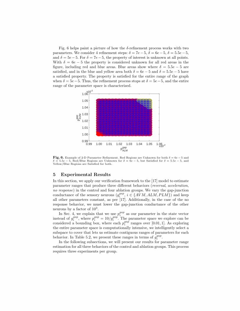
Fig. 6 helps paint a picture of how the δ-refinement process works with twoparameters. We consider 4 refinement steps: δ = 7e− 5, δ = 6e− 5, δ = 5.5e− 5,and δ = 5e− 5. For δ = 7e− 5, the property of interest is unknown at all points.With δ = 6e − 5 the property is considered unknown for all red areas in thefigure, including red and blue areas. Blue areas show where δ = 5.5e − 5 aresatisfied, and in the blue and yellow area both δ = 6e− 5 and δ = 5.5e− 5 havea satisfied property. The property is satisfied for the entire range of the graphwhen δ = 5e−5. Thus, the refinement process stops at δ = 5e−5, and the entirerange of the parameter space is characterized.

pgapALM

0.99 1.00 1.01 1.02 1.03 1.04 1.05 1.06

pgap

AV

M

0.99

1.00

1.01

1.02

1.03

1.04

1.05

1.06

x10-2

x10-2

Fig. 6. Example of 2-D Parameter Refinement. Red Regions are Unknown for both δ = 6e− 5 andδ = 5.5e − 5, Red/Blue Regions are Unknown for δ = 6e − 5, but Satisfied for δ = 5.5e − 5, andYellow/Blue Regions are Satisfied for both.

5 Experimental Results

In this section, we apply our verification framework to the [17] model to estimateparameter ranges that produce three different behaviors (reversal, acceleration,no response) in the control and four ablation groups. We vary the gap-junctionconductance of the sensory neurons (ggapi , i ∈ {AVM,ALM,PLM}) and keepall other parameters constant, as per [17]. Additionally, in the case of the noresponse behavior, we must lower the gap-junction conductance of the otherneurons by a factor of 103.

In Sec. 4, we explain that we use pgapi as our parameter in the state vectorinstead of ggapi , where pgapi = 10/ggapi . The parameter space we explore can beconsidered a bounding box, where each pgapi ranges over [0.01, 1]. As exploringthe entire parameter space is computationally intensive, we intelligently select asubspace to cover that lets us estimate contiguous ranges of parameters for eachbehavior. In Table 5.2, we present these ranges in terms of ggapi .

In the following subsections, we will present our results for parameter rangeestimation for all three behaviors of the control and ablation groups. This processrequires three experiments per group.

5.1 1-D Parameter SpaceHere we vary pgapAVM in all groups, except the AVM,ALM- group. By varyingthis parameter, we are able to produce reversal behavior in all four groups. Weare also able to produce acceleration in all groups but PLM-. The PLM neurondrives acceleration in the TW circuit [16]. Hence, its absence in the PLM- groupprevents acceleration from being produced, justifying the result.

For the AVM,ALM- group, we vary pgapPLM and produce acceleration and noresponse behaviors. As both AVM and ALM, responsible for reversal of move-ment, are ablated, reversal cannot be produced by this group.

5.2 2-D Parameter SpaceIn this set of experiments, we vary two parameters simultaneously. First we varypgapAVM and pgapALM for the control and PLM- groups. In both cases we producereversal behavior. For the same reasons given in the previous subsection, we areunable to produce acceleration in the PLM- group and no response behavior inboth these groups.

Next, we vary pgapAVM and pgapPLM for the ALM- and ALM,DVA- groups. Weare able to produce both all three behaviors in both groups.

5.3 3-D Parameter SpaceSince the ablation groups we have used in this paper all feature at least one ofthe primary sensory neurons (ALM, AVM, and PLM ) ablated, we can only showthe 3-D case for the original animal.

For the 3-D case, in addition to pgapAVM and pgapALM , we have the pgapPLM con-ductance. Finally, we get a non-zero value for no response in the control, butTable 5.2 shows that this value is an order of magnitude smaller than accelerationand several orders smaller than reversal.

5.4 Runtime and Memory Complexity AnalysisThe time and memory needed for the procedure depends upon the value of δused and the size of the parameter space. Assume Ld to be the interval length inthe dth dimension. The total number of δ-balls required to cover the parameterspace completely is:

TN = ΠDd=1Nd

where D is the number of parameters added to the state vector and Nd = 2Ld/δ.If Ld is the same in all dimensions, TN = ND

d . We can analyze both runtime andmemory complexity based on TN . If we consider the time and memory requiredfor verifying each δ-ball to be O(1), then the time and memory complexity willboth be O(TN ) = O(ND

d ). Note that the complexity also depends on the valueof the δ-refinement loop counter. Since we can safely assume that the loop williterate only a constant number of times, this is not an issue.

Fig. 7 illustrates how runtime relates to TN in one (a) and multiple (b)dimensions. The graph from (a) is the same as the 1D line in (b), but for a largerrange of TN . This increased range more clearly illustrates the linear relationshipof runtime to TN when D = 1. Part (b) shows the rates for D = 1, D = 2 andD = 3 over a much smaller range of TN but helps to demonstrate the effectof dimensionality on time complexity. Since runtime grows at a trinomial rate

Group Name Property Parameters Ranges δ Runtime (sec)

Control

REV ggapAV M [46.2, 1000] 1e− 6 6324.4REV ggapAV M , ggapALM [952.38, 1000]2 2e− 5 776.5REV ggapAV M , ggapALM , ggapALM [990.01, 1000]3 2e− 5 314.23ACC ggapAV M [15.87, 10] 1e− 5 1110.01ACC ggapAV M , ggapALM [15.86, 15.87]2 2e− 5 1619.8ACC ggapAV M , ggapALM , ggapALM [15.85, 15.87]3 2e− 5 320.12NR ggapAV M - - -NR ggapAV M , ggapALM - - -NR ggapAV M , ggapALM , ggapALM [10.005, 10]3 5e− 5 124.23

PLM-

REV ggapAV M [467.3, 1000] 1e− 5 718.08REV ggapAV M , ggapALM [952.38, 1000]2 2e− 5 775.12ACC ggapAV M - - -ACC ggapAV M , ggapALM - - -NR ggapAV M - - -NR ggapAV M , ggapALM [15.84, 15.87]2 5e− 5 124.23

ALM-

REV ggapAV M [467.3, 1000] 1e− 5 718.08REV ggapAV M , ggapPLM [952.38, 1000]2 2e− 5 785.01ACC ggapAV M [15.38, 15.87] 2e− 5 660.87ACC ggapAV M , ggapPLM [14.91, 14.93]2 2e− 5 782.3NR ggapAV M - - -NR ggapAV M , ggapPLM [10, 10.05]2 5e− 5 125.01

ALM,DVA-

REV ggapAV M [250, 500] 1e− 5 1085.74REV ggapAV M , ggapPLM [487.80, 500]2 2e− 5 779.75ACC ggapAV M [13.88, 14.28] 1e− 5 1084.23ACC ggapAV M , ggapPLM [15.84, 15.87]2 2e− 5 782.3NR ggapAV M - - -NR ggapAV M , ggapPLM [15.86, 15.87]2 2e− 5 779.01

ALM,AVM-REV ggapPLM - - -ACC ggapPLM [33.33, 1000] 5e− 5 3619.19NR ggapPLM , ggapALM [10, 13.33] 5e− 5 3118.45

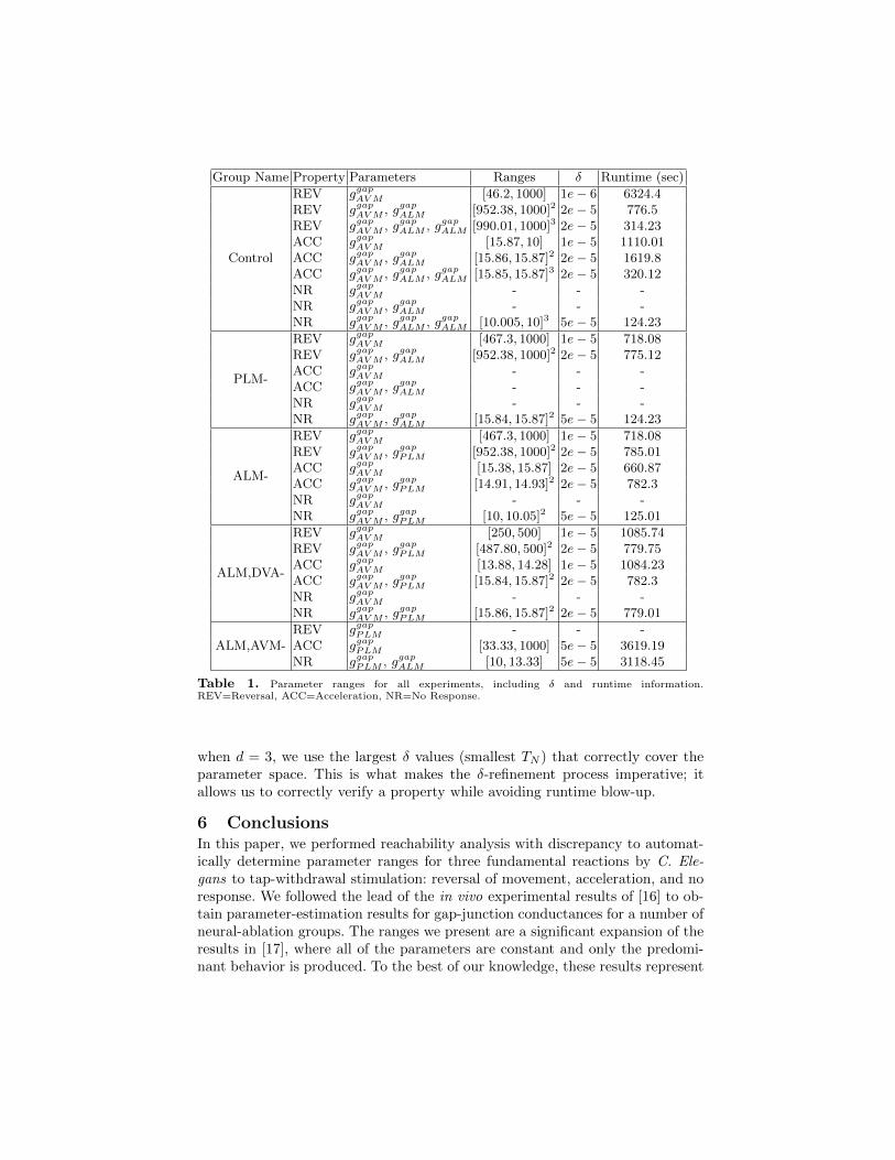
Table 1. Parameter ranges for all experiments, including δ and runtime information.REV=Reversal, ACC=Acceleration, NR=No Response.

when d = 3, we use the largest δ values (smallest TN ) that correctly cover theparameter space. This is what makes the δ-refinement process imperative; itallows us to correctly verify a property while avoiding runtime blow-up.

6 ConclusionsIn this paper, we performed reachability analysis with discrepancy to automat-ically determine parameter ranges for three fundamental reactions by C. Ele-gans to tap-withdrawal stimulation: reversal of movement, acceleration, and noresponse. We followed the lead of the in vivo experimental results of [16] to ob-tain parameter-estimation results for gap-junction conductances for a number ofneural-ablation groups. The ranges we present are a significant expansion of theresults in [17], where all of the parameters are constant and only the predomi-nant behavior is produced. To the best of our knowledge, these results represent

0 1000 2000 3000 4000 5000 6000 70000

500

1000

1500

2000

2500

Total points (TN)

Ru

ntim

e (

s)

(a) Runtime analysis over TN

0 5 10 15 20 25 300

1000

2000

3000

4000

5000

6000

7000

8000

9000

Points in each dimension (ND)

Ru

ntim

e (

s)

1D2D3D

(b) Runtime analysis over dimension

Fig. 7. Experiment on runtime analysis.

the first formal verification of a biologically realistic (nonlinear ODE) model ofa neural circuit in a multicellular organism.

The verification framework we develop is model-agnostic, and allows the tech-niques of [6] to be applied to general nonlinear ODE models. This is only possiblethrough the careful model and verification engineering developed in this paper.

As alluded in Sec. 5, our results cannot necessarily cover the entire param-eter space due to the TN required, but still enough to verify the properties inquestion. A potential solution to the incomplete coverage is parallelizing ourapproach. Luckily, calculating reach-tubes is a data-parallel computation andconsidered “trivially parallel” for the GPGPU (General-Purpose computing ona Graphics Processing Unit) architecture. This should allow us to run verifica-tion experiments in a fraction of the current required time, giving us a potentialexpansion of coverage.

Acknowledgments. We would like to thank Junxing Yang, Heraldo Memelli,Farhan Ali, and Elizabeth Cherry for their numerous contributions to this project.Our research is supported in part by the following grants: NSF IIS 1447549,NSF CAR 1054247, AFOSR FA9550-14-1-0261, AFOSR YIP FA9550-12-1-0336,CCF-0926190, and NASA NNX12AN15H.

References

1. M. Chalfie, J. E. Sulston, J. G. White, E. Southgate, J. N. Thomson, and S. Bren-ner. The neural circuit for touch sensitivity in Caenorhabditis Elegans. The Journalof Neuroscience, 5(4):956–964, 1985.

2. A. Donze and O. Maler. Systematic simulation using sensitivity analysis. In HybridSystems: Computation and Control, pages 174–189. Springer, 2007.

3. P. S. Duggirala, S. Mitra, and M. Viswanathan. Verification of annotated mod-els from executions. In Proceedings of the International Conference on EmbeddedSoftware, EMSOFT 2013, Montreal, Canada, Sep.-Oct. 2013. IEEE.

4. P. S. Duggirala, S. Mitra, M. Viswanathan, and M. Potok. C2E2: A verification toolfor Stateflow models. In 21st International Conference on Tools and Algorithmsfor the Construction and Analysis of Systems, TACAS 2015, 2015.

5. P. S. Duggirala, L. Wang, S. Mitra, M. Viswanathan, and C. Munoz. Temporalprecedence checking for switched models and its application to a parallel landingprotocol. In FM 2014: Formal Methods, 19th International Symposium, Proceed-ings, volume 8442 of Lecture Notes in Computer Science, pages 215–229. Springer,May 2014.

6. C. Fan and S. Mitra. Bounded verification using on-the-fly discrepancy compu-tation. Technical Report UILU-ENG-15-2201, Coordinated Science Laboratory,University of Illinois at Urbana-Champaign, Feb. 2015.

7. R. Grosu, G. Batt, F. H. Fenton, J. Glimm, C. L. Guernic, S. A. Smolka, andE. Bartocci. From cardiac cells to genetic regulatory networks. In Proceedings ofthe 23rd International Conference on Computer Aided Verification, pages 396–411.Springer, 2011.

8. A. L. Hodgkin and A. F. Huxley. A quantitative description of membrane currentand its application to conduction and excitation in nerve. Journal of Physiology,117:500–544, 1952.

9. Z. Huang, C. Fan, A. Mereacre, S. Mitra, and M. Z. Kwiatkowska. Invariantverification of nonlinear hybrid automata networks of cardiac cells. In ComputerAided Verification, 26th International Conference, CAV 2014, Proceedings, volume8559 of Lecture Notes in Computer Science, pages 373–390, Vienna, Austria, July2014. Springer.

10. M. A. Islam, A. Murthy, A. Girard, S. A. Smolka, and R. Grosu. Composition-ality results for cardiac cell dynamics. In Proceedings of the 17th InternationalConference on Hybrid Systems: Computation and Control. ACM, 2014.

11. S. M. Iyengar, C. Talcott, R. Mozzachiodi, E. Cataldo, and D. A. Baxter. Exe-cutable symbolic models of neural processes.

12. W. Lohmiller and J. J. E. Slotine. On contraction analysis for non-linear systems.Automatica, 1998.

13. A. Murthy, M. A. Islam, R. Grosu, and S. A. Smolka. Computing bisimulationfunctions using SOS optimization and delta-decidability over the reals. In Proceed-ings of the 18th International Conference on Hybrid Systems: Computation andControl. ACM, 2015.

14. A. Tiwari and C. L. Talcott. Analyzing a discrete model of Aplysia central patterngenerator. In Proceedings of the 6th Conference on Computational Methods inSystems Biology (CMSB), pages 347–366. Springer, 2008.

15. L. R. Varshney. Individual differences. http://blog.openworm.org/post/

107263481195/individual-differences, 2015.16. S. R. Wicks and C. H. Rankin. Integration of mechanosensory stimuli in

Caenorhabditis Elegans. The Journal of Neuroscience, 15(3):2434–2444, 1995.17. S. R. Wicks, C. J. Roehrig, and C. H. Rankin. A dynamic network simulation

of the nematode tap withdrawal circuit: Predictions concerning synaptic functionusing behavioral criteria. The Journal of Neuroscience, 16(12):4017–4031, 1996.