1

Abstract

The Ambient Calculus is a process calculus where processes may re-side within a hierarchy of locations and modify it. The purpose of thecalculus is to study mobil ity, which is seen as the change of spatialconfigurations over time. In order to describe properties of mobilecomputations we devise a modal logic that can talk about space aswell as time, and that has the Ambient Calculus as a model.

1 Introduction

In the course of our ongoing work on mobili ty [3,4,5,12], we haveoften struggled to express precisely certain properties of mobilecomputations. Informally, these are properties such as “ the agent hasgone away”, “eventually the agent crosses the firewall” , “everyagent always carries a suitcase” , “somewhere there is a virus” , or“ there is always at most one agent called n here” . There are severalconceivable ways of formalizing these assertions. It is possible toexpress some of them in terms of equations [12], but this is some-times diff icult or unnatural. It is easier to express some of them asproperties of computational traces, but this is very low-level.

Modal logics (particularly, temporal logics) have emerged inmany domains as a good compromise between expressiveness andabstraction. In addition, many modal logics support useful computa-tional applications, such as model checking. In our context, it makessense to talk about properties that hold at particular locations, and itbecomes natural to consider spatial modali ties for properties thathold at a certain location, at some location, or at every location.

Space

Interesting spatial structures can be represented conveniently as un-ordered edge-labeled trees, where edge labels correspond to namesof sublocations, and subtrees correspond to sublocations. Such a rep-resentation of locations is shared by the Ambient Calculus [3], theDistributed Join Calculus [10], the Seal Calculus [20], and triviallyby the many distributed process calculi with a flat location structure(e.g.: [2]).

The following edge-labeled tree represents two contiguous lo-cations, a and b, such that b has no sublocations, and a has a sublo-cation called p. The diagram on the right gives a more intuitive butequivalent description of location contiguity and containment:

In the Ambient Calculus, contiguous locations (or processes)are represented by standard parallel composition (P | Q), and namedlocations are represented by ambients (n[P]) which name a locationn with contents P. This fragment of the Ambient Calculus, togetherwith a void process (0) and simple syntactic equivalences, amountsto a textual representation of edge-labeled trees. The example abovecould be written as a[p[0]] | b[0], assuming there are no active pro-cesses within the locations.

Even before considering process execution, we can talk aboutspatial properties and spatial specifications. For example, we havethe following correspondence between spatial constructs in the Am-bient Calculus and certain formulas of the logic we develop later:

We have a logical constant 0 that is satisfied by the process 0 repre-senting void. We have logical propositions of the form n[$] (mean-ing that $ holds at location n) that are satisfied by processes of theform n[P] (meaning that process P is located at n) provided that Psatisfies $. We have logical propositions of the form $ | % (mean-ing that $�and %�hold contiguously) which are satisfied by contigu-ous processes of the form P | Q if P satisfies $�and Q satisfies %, orvice versa.

Time

Spatial configurations evolve over time as a consequence of the ac-tivities of processes. For example, our initial tree may go through thefollowing two steps of evolution, as the result of a process movingthe location p from a to b through the ether in between.

Permission to make digita/hard copies of all or part of this material for personal or class-room use is granted without fee provided that the copies are not made or distributed for profit or commercial advantage, the copyright notice, the title of the publication and its date appear, and notice is given that copyright is by permission of the ACM, Inc. To copy otherwise, to republish, to post on servers or to redistribute to lists, requires spe-cific permission and/or fee.POPL 2000, Boston, USA.© 2000 ACM.

Processes0n[P]P | Q

(void)(location)(composition)

Formulas0n[$]$ | %

(there is nothing here)(there is one thing here)(there are two things here)

a b

p

pa b

Î

a bp

Î

a b

p

Anytime, AnywhereModal Logics for Mobile Ambients

Luca Cardelli, Andrew D. Gordon

Microsoft Research

2

We can think of processes as sitting at the nodes of edge-labeledtrees, and directing the movement of those nodes through the trees.So, the steps above could be caused by a process executing move-ment instructions at the node under p.

Mobility

We regard mobili ty as the evolution of spatial configurations overtime. A specification logic for mobil ity should be able to talk aboutthe structure of spatial configurations and about their evolutionthrough time; that is, it should be a modal logic of space and time.

A typical specification would say that the configuration looksinitially like a certain tree, and eventually li ke some other tree. Insome cases we may want to be very precise about describing thestructure of locations, even though this runs against the traditionalattitude in logics for process calculi that prevents “counting” thenumber of processes (or locations) involved. Our logic can be veryspecific, in this sense.

Of course, since we are dealing with specifications, we mayalso want to be able to be imprecise, and describe things that happen“somewhere” or “sometime”. Rarely, though, we want to be veryprecise about particular execution steps, so that the same flavor oflogic of mobility seems applicable to a variety of calculi. In fact, thenotion of mobil ity as evolution of location trees is shared by severalcalculi, including Ambients, Join, and Seal, although the mechanismand properties of mobili ty steps differ greatly between them.

In this paper, we concentrate on the Ambient Calculus for con-creteness, but our main thrust is applicable to any distributed processcalculus that includes a hierarchical and dynamic structure of loca-tions.

Paper Outline

Spatial modali ties have an intensional flavor that distinguishes ourlogic from other modal logics for concurrency. Previous work in thearea concentrates on properties that are invariant up to strong equiv-alences such as bisimulation [15,6], while our properties are invari-ant only up to simple spatial rearrangements. Some of our tech-niques can be usefully applied to other process calculi, even onesthat do not have locations, such as CCS.

We start from a computational basis: a process calculus, sum-marized in Section 2, that acts as a model for the logic. In Section 3we introduce logical formulas and a notion of satisfaction. In Section4, we derive logical inference rules, including rules for time, space,and satisfiability modalities, and novel rules for locations and pro-cess composition (the rules are summarized in the Appendix). At theend of this section we give a detailed example of logical inference.In Section 5 we investigate model checking of mobile programs, onthe basis of the satisfaction relation between processes and formulas.Finally, in Section 6, we compare our logic with relevant and linearlogics.

2 The Ambient Calculus with Public Names

In this paper we consider only ambients having public names; that iswe do not deal with name restriction and scope extrusion. Handlingof private names in a logic is a very interesting topic, but we leave itfor future work.

2.1 Ambients

We summarize a modified version of the basic Ambient Calculus of[3]. The changes consist in removing name restriction, and in

strengthening the definition of structural congruence so that it char-acterizes the intended equivalence on spatial configurations.

The following table summarizes the syntax of processes. Wehave separated the process constructs into spatial and temporal; thisis similar to the distinction between static and dynamic constructs inCCS [17]. This paper focuses on the spatial constructs; the temporalconstructs and the dynamic behavior are necessary but secondary forour current purposes.

Processes

The set of free names of a process P, written fn(P), is defined as usu-al; the only binder is in the input action. We write P{ n←M} for thesubstitution of the message M for each free occurrence of the namen in the process P. Similarly for M{ n←M’ } . The 0 process is oftenomitted in the contexts n[0] and M.0, yielding n[] and M.

2.2 Structural Congruence and Reduction

Structural congruence is a relation between processes; it is usedheavily in the logic, as well as in the reduction semantics. Intuitively,structural congruence equates processes up to simple “rearrange-ment” of parts, without any computational significance. We canidentify five groups of rules in the following table: for equivalence,for congruence of spatial operators, for composition, for replication,and for temporal operators and paths.

Structural Congruence

P,Q,R ::=0P | Q!PM[P]M.P(n).PjMk

processesvoidcompositionreplicationambientcapabil ity actioninput actionoutput action

M ::=nin Mout Mopen MεM.M’

messagesnamecan enter into Mcan exit out of Mcan open Mnullcomposite

P � PP � Q ⇒ Q � PP � Q, Q � R ⇒ P � R

P � Q ⇒ P | R � Q | RP � Q ⇒ !P � !QP � Q ⇒ M[P] � M[Q]

P | Q � Q | P(P | Q) | R � P | (Q | R)P | 0 � P

(Struct Refl)(Struct Symm)(Struct Trans)

(Struct Par)(Struct Repl)(Struct Amb)

(Struct Par Comm)(Struct Par Assoc)(Struct Par Zero)

!(P | Q) � !P | !Q!0 � 0!P � P | !P!P � !!P

(Struct Repl Par)(Struct Repl Zero)(Struct Repl Copy)(Struct Repl Repl)

spatial

temporal

capabilities

paths

names

3

Spatial configurations are ambient configurations consistingonly of spatial operators. For example, a[b[0] | !c[0 | 0] | !0] is a spa-tial configuration. These configurations have a natural interpretationas edge-labeled finite-depth trees, where replication introduces infi-nite branching. The rules for structural congruence are sound andcomplete for equivalence of these trees. We do not elaborate this fur-ther, but it suffices to say that this completeness result motivates thechoice of axioms for structural congruence, and particularly the ax-ioms for replication (which are the same as in Engelfriet’s work onthe π-calculus [9]).

Reduction

The reduction relation describes the dynamic behavior of am-bients. In particular, the rules (Red In), (Red Out) and (Red Open)represent mobility, while (Red Comm) represents local communica-tion (see [3] for an extended discussion). For example, the process:

represents a packet p that travels out of host a and into host b, whereit is opened, and its contents m are read and used to create a new am-bient. The process reduces in four steps (illustrating each of the fourreduction rules) to the residual process a[] | b[m[] ]. The first threestates correspond to the tree diagrams in the Introduction.

2-1 Facts about Structural Congruence(1) P | Q ����0 iff P ����0 and Q ����0.

(2) n[P] #�0.

(3) n[P] ��Q | R iff either Q ��n[P] and R ��0, or Q ��0 and R ��n[P].

(4) m[P] �� n[Q] iff m = n and P �� Q.

(5) m[P] | n[Q] ��m’ [P’ ] | n’ [Q’ ] iff either m = m’ , n = n’ , P � P’ ,Q � Q’ , or m = n’ , n = m’ , P � Q’ , Q � P’ .

1

3 The Logic

In a modal logic, the truth of a formula is relative to a state (orworld). In our case, the truth of a space-time modal formula is rela-tive to the here and now. Each formula talks about the current time,that is, the current state of execution, and the current place, that is,the current location. For example, the formula n[0] is read: there is

here and now an empty location called n. The operator n[$] repre-sents a single step in space, allowing us to talk about the place onestep down into n. Another operator, �$, allows us to talk about anarbitrary number of steps in space; this is akin to the temporal even-tuality operator, 2$.

3.1 Logical Formulas

The syntax of logical formulas is summarized below. This is a modalpredicate logic with classical negation. As usual, many standardconnectives are interdefinable. The meaning of the formulas wil l begiven shortly in terms of a satisfaction relation. Informally, the firstthree formulas (true, negation, disjunction) give propositional logic.The next three (void, location, composition) capture spatial config-urations, as we discussed. Then we have quantification over names,the two temporal and spatial modalities, and two further operatorsthat we explain later. Quantified variables range only over names:these variables may appear in the location and location adjunct con-structs.

Logical Formulas

The free names of a formula, fn($), are easily defined since there areno name binders. The free variables of a formula, fv($), are definedalong standard lines: only quantifiers bind variables. A formula $ isclosed if fv($) = Ô.

3.2 Satisfaction

The satisfaction relation P � $�means that the process P satisfies theclosed formula $. This relation is defined inductively in the follow-ing table, where Π is the sort of processes, Φ is the sort of formulas,ϑ is the sort of variables, and Λ is the sort of names. We are very ex-plicit about quantification and sorting of meta-variables because ofsubtle scoping issues, particularly in the definition of P � Òx.$. Weuse the same syntax for logical connectives at the meta-level and ob-ject-level, but this is unambiguous.

The meaning of the temporal modality is given by reductions inthe operational semantics of the Ambient Calculus. For the spatialmodality, we need the following definition: the relation P�P’ indi-cates that P contains P’ within exactly one level of nesting; that is,P’ is one step away from P in space, in some downward direction.

Then, P�*P’ is the reflexive and transitive closure of the previous re-lation, indicating that P contains P’ at some nesting level. Note thatP’ consists of either the top level P, or the entire contents of an en-closed ambient.

P � Q ⇒ M.P � M.QP � Q ⇒ (x).P � (x).Q

(Struct Action)(Struct Input)

ε.P � P(M.M’ ).P � M.M’ .P

(Struct ε)(Struct .)

n[in m. P | Q] | m[R] xyyz m[n[P | Q] | R] (Red In)m[n[out m. P | Q] | R] xyyz n[P | Q] | m[R] (Red Out)open n. P | n[Q] xyyz P | Q (Red Open)(n).P | jMk xyyz P{ n←M} (Red Comm)P xyyz Q ⇒ n[P] xyyz n[Q] (Red Amb)P xyyz Q ⇒ P | R xyyz Q | R (Red Par)P’ � P, P xyyz Q, Q � Q’ ⇒ P’ xyyz Q’ (Red �)xyyz* is the reflexive and transitive closure of xyyz

a[p[out a. in b. jmk]] | b[open p. (x). x[]]

a[p[out a. in b. jmk]] | b[open p. (x). x[]]xyyz a[] | p[in b. jmk] | b[open p. (x). x[]] (Red Out)xyyz a[] | b[p[jmk] | open p. (x). x[]] (Red In)xyyz a[] | b[jmk | (x). x[]] (Red Open)xyyz a[] | b[m[]] (Red Comm)

η is a name n or a variable x

$, %, & ::=T true¬$ negation$ ∨ % disjunction0 voidη[$] location$ | % compositionÒx.$ universal quantification over names2$ sometime modality�$ somewhere modali ty$@η location adjunct$©% composition adjunct

P�P’ iff Ón, P” . P � n[P’ ] | P”

4

Satisfaction

We spell out some of these definitions. A process P satisfies theformula n[$] if there exists a process P’ such that P has the shapen[P’ ] with P’ satisfying $. A process P satisfies the formula $ª | $¨if there exist processes P’ and P” such that P has the shape P’ | P”with P’ satisfying $ª and P” satisfying $¨. A process P satisfies theformula 2$ if $ holds in the future for some residual P’ of P, where“residual” is defined by Pxyz*P’ . A process P satisfies the formula�$ if $ holds at some sublocation P’ within P, where “sublocation”is defined by P�*P’ .

The last two connectives, @ and ©, can be used to express as-sumption/guarantee specifications [1]; they were inspired by thewish to express security properties. A reading of P � $@n is that P(together with its context) manages to satisfy $ even when placedinto a location called n. A reading of P � $©% is that P (togetherwith its context) manages to satisfy % under any possible attack byan opponent that is bound to satisfy $. Moreover, P � (4$)©(4$)can be interpreted as saying that P preserves the invariant $. We willsee that these two connectives arise as natural adjuncts to the loca-tion and composition connectives, respectively.

The definition of satisfaction is based heavily on the structuralcongruence relation. This use of structural congruence may appeararbitrary: other equivalence relations could be used in its place. Wehave tried to motivate the choice of structural congruence by dis-cussing in Section 2.2 how structural congruence precisely capturesthe intuition of ambients as spatial configurations. Moreover, struc-tural congruence is easily decidable, which is useful in model-checking applications (see Section 5).

The following table lists some derived connectives, illustratingsome properties that can be expressed in the logic. The informalmeanings can be understood better by expanding out the definitionsfrom the table above. Some discussion follows.

Der ived Connectives

Syntactic conventions: ‘©’ , ‘2’ , ‘4’ , ‘�’ , and ‘�’ bind more strong-ly than ‘ |’ ; and they all bind more strongly than the standard logicalconnectives, which have standard precedences. Quantifiers extendto the right as far as possible.

Decomposition is the DeMorgan dual of composition. A de-composition formula $ || % is satisfied if for every parallel decom-position of the process in question, either one component satisfies $or the other satisfies %. Then, $Ò means that in every decompositioneither one component satisfies $ or the other satisfies F; since thelatter is impossible, in every possible decomposition one componentmust satisfy $. For example: (n[T]⇒n[m[T]])Ò means that everyambient n that can be found here contains a single subambient m.The DeMorgan dual of $Ò is $Ó, which means that it is possible tofind a decomposition where one component satisfies $. For exam-ple, n[m[T]Ó]Ó means that there is at least one ambient n here thatcontains at least one subambient m.

Other operators are derived as DeMorgan duals: existentialquantification, and everytime and everywhere modalities. Examplesfor these modalities are: 4n[T] (there is always a location called nhere), and �¬(n[T]Ó) (there is now no location called n anywhere).

Fusion, $ ∝ %, is an operator that arises in relevant logic (when© is seen as relevant implication). In our context, $ ∝ % means thatthere is a context satisfying %�that helps ensuring $. The adjunct offusion, $ |⇒ %, turns out to be very natural in specifications: itmeans that in every decomposition, if one part satisfies $, then theother part must satisfy %.

The following is a fundamental property of the satisfaction re-lation; it states that satisfaction is invariant under structural congru-ence of processes. In other words, logical formulas can only expressproperties that are invariant up to structural congruence. The proofis a simple induction on the structure of $.

3-1 Proposition (Satisfaction is up to �)(P � $�∧ P � P’ ) ⇒ P’ � $

1We end this section with an example of a proof that a certain

process satisfies a certain formula. A proof of even a very simplenegative formula requires techniques for analyzing the derivation ofstructural congruences. For example, consider proving the followingassertion, where m ≠ n:

For a contradiction, suppose that m[] | n[] � Óx. x[T] | x[T]. Bydefinition, this means there is a P such that m[] | n[] � P and there isa q with P � q[T] | q[T]. This implies that there are processes P’ andP” such that m[] | n[] ��P’ | P” with P’ � q[T] and P” � q[T]. Inturn, P’ � q[T] implies there is Q’ such that P’ ��q[Q’ ]. Similarly,P” � q[T] implies there is Q” such that P” ��q[Q” ]. In summary:

According to the Fact 2-1(5), there are two ways in which this equa-tion can have been derived. In either case, it follows that m = q andn = q, and therefore m = n. This yields the desired contradiction, aswe are assuming that m ≠ n.

ÒP:Π.ÒP:Π, $:Φ.

P � TP � ¬$ $ ¬ P � $

ÒP:Π, $,%:Φ. P � $∨% $ P � $ ∨ P � %

ÒP:Π.ÒP:Π, n:Λ, $:Φ.ÒP:Π, $,%:Φ.

ÒP:Π, x:ϑ, $:Φ.ÒP:Π, $:Φ.ÒP:Π, $:Φ.

P � 0P � n[$]P � $ | %

P � Òx.$P � 2$

P � �$

$ P � 0$ ÓP’ :Π. P � n[P’ ] ∧ P’ � $$ ÓP’ ,P” :Π. P � P’ |P”

∧ P’ � $ ∧ P” � %$ Òm:Λ. P � ${ x←m}$ ÓP’ :Π. Pxyz*P’ ∧ P’ � $$ ÓP’ :Π. P�*P’ ∧ P’ � $

ÒP:Π, $:Φ.ÒP:Π, $,%:Φ.

P � $@nP � $©%

$ n[P] � $ $ ÒP’ :Π. P’ � $ ⇒ P|P’ � %

F $ ¬T$ ∧ % $ ¬(¬$ ∨ ¬%)

falseconjunction

$ ⇒ % $ ¬$ ∨ % implication$ ⇔ % $ ($ ⇒ %) ∧ (% ⇒ $) logical equivalence$ || % $ ¬(¬$ | ¬%)$Ò $ $ || F$Ó $ $ | TÓx.$ $ ¬Òx.¬$

decompositionevery component satisfies $some component satisfies $existential quantification

4 $ $ ¬2¬$

�$ $ ¬�¬$

everytime modalityeverywhere modality

$ ∝ % $ ¬(% © ¬$)$ |⇒ % $ ¬($ | ¬%)

fusionfusion adjunct

m[] | n[] � ¬ Óx. x[T] | x[T]

m[] | n[] ��q[Q’ ] | q[Q” ]

5

4 Validity

In this section, we study valid formulas, valid sequents, and validlogical inference rules. All these are based on the satisfaction rela-tion given in the previous section. Once the definition of satisfactionis fixed, we are basically committed to whatever logic comes out ofit. Therefore, it is important to stress that the satisfaction relation ap-pears very natural to us. In particular, the definitions of 0, n[$], and$ | % seem inevitable, once we accept that formulas should be ableto talk about the tree structure of locations, and that they should notdistinguish processes that are surely indistinguishable (up to �). Theconnectives $@n and $©%�have natural security motivations. Themodalities 2$�and �$�talk about process evolution and structure inan undetermined way, which is good for mobility specifications. Therest is classical predicate logic, with the ability to quantify over lo-cation names.

Through the satisfaction relation, our logic is based on solidcomputational intuitions. We should now approach the task of dis-covering the rules of the logic without preconceptions. As we shallsee, what we get has famil iar as well as novel aspects.

4.1 The Meaning of Rules

A closed formula is valid if it is satisfied by every process. (For themoment, we consider only validity for closed formulas, i.e., propo-sitional validity.) We use validity for interpreting logical inferencerules, as described in the next definition. We use a linearized nota-tion for inference rules, where the usual horizontal bar separating an-tecedents from consequents is written ‘’ in-line, and ‘ ;’ is used toseparate antecedents.

Validity, Sequents, and Rules

We adopt a non-standard formulation of sequents, where eachsequent has exactly one assumption and one conclusion: $�L} %. Ourintention in doing so is to avoid pre-judging the interpretation of thestructural operator “ ,” in standard sequents. In our logic, by taking ∧on the left and ∨ on the right of�L} as structural operators (i.e., as “ ,” ),all the standard rules of sequent and natural deduction systems withmultiple premises/conclusions can be derived. Instead, by taking | onthe left of�L} as a structural operator, all the rules of intuitionistic lin-ear logic can be derived. Finally, by taking nestings of ∧ and | on theleft of L} as structural “bunches” , we obtain a bunched logic [18]. Wediscuss this further in Section 6.

Noticeably, we abandon Gentzen’s distinction between struc-tural rules and other logical rules, which has been a staple of formallogic since [11]. We do not see this as a fundamental or irrevocablestep. Not all l ogics fit easily into Gentzen’s initial approach, andmany alternative sequent structures have been studied [7]. There-

fore, there may be formulations of our logic which identify a set ofstructural rules, perhaps along the lines of [18]. At the current stagein the development of our logic, however, it is unclear how to pro-ceed in that direction.

4.2 Rules of the Logic

In the sequel, we organize our results into tables of Rules, which arevalidated in the model, and into tables of Corollaries, which are de-rived purely logically from the inference rules.

4.2.1 Propositions

The following is a non-standard presentation of the propositional se-quent calculus [14], based on our single-assumption single-conclu-sion sequents. In this presentation, the rules of propositional logicbecome very symmetrical, and many proofs become more regular,having to consider only single formulas instead of sequences of for-mulas.

Propositional Rules

The standard deduction rules of propositional logic, both for the se-quent calculus and for natural deduction (interpreting “ ,” as ∧ on theleft and ∨ on the right), are derivable from the rules in the table.

4.2.2 Composition

The logical rules of composition apply not only to our calculus butalso to any calculus that includes a standard process composition op-erator, for example, CCS.

Composition Rules

The first two rules assert that 0 is part of any process, and thatif a part is non-0 so is the whole. The next three rules give associa-tivity, commutativity, and congruence of composition.

The converse of the |-∨ distribution rule ( | ∨), namely $ | &�∨% | & L} ($∨%) | &, is derivable. So is a |-∧ distribution rule, ($∧%)

vld($) $ ÒP:Π. P � $ Validity for (closed) $

$�L} % $ vld($ ⇒ %) Sequent

$�xML} % $ $�L} % ∧ %�L} $ Double Sequent

$1�L} %1; ...; $n�L} %n� $0�L} %0 $ Inference Rule (n≥0)$1�L} %1 ∧ ... ∧ $n�L} %n ⇒ $0�L} %0

$1�L} %1; ...; $n�L} %n� $�xML} % $ Double Conclusion$1�L} %1 ∧ ... ∧ $n�L} %n ⇒ $0�xML} %0

$1�L} %1 $2�L} %2 $ Double Rule$1�L} %1 $2�L} %2 ∧ $2�L} %2 $1�L} %1

(A-L) $∧(&∧')�L} % ($∧&)∧'�L} %(A-R) $�L} (&∨')∨% $�L} &∨('∨%)(X-L) $∧&�L} % &∧$�L} %(X-R) $�L} &∨% $�L} %∨&(C-L) $∧$�L} % $�L} %(C-R) $�L} %∨% $�L} %(W-L) $�L} % $∧&�L} %(W-R) $�L} % $�L} &∨%(Id) $�L} $(Cut) $�L} &∨%; $ª∧&�L} %ª $∧$ª�L} %∨%ª

(T) $∧T�L} % $ L} %(F) $�L} F∨% $ L} %(¬-L) $�L} &∨% $∧¬&�L} %(¬-R) $∧&�L} % $�L} ¬&∨%

( | 0) $ | 0 xML} $( | ¬0) $ | ¬0 L} ¬0(A | ) $ | (% | &) xML} ($ | %) | &(X | ) $ | % L} % | $( | L}) $ª�L} %ª; $¨�L} %¨ $ª | $¨ L} %ª | %¨

( | ∨) ($∨%) | & L} $ | &�∨ % | &( | || ) $ª | $¨ L} ($ª | %¨)�∨ (%ª | $¨)�∨ (¬%ª | ¬%¨)( | ©) $ | &�L} % $�L} &©%

6

| & L} $ | &�∧ % | &. However, the converse of that, namely $ | &�∧ %| & L} ($∧%) | &, is not sound. (Take $ = n[m[T]], % = n[p[T]] , & =n[T], and P = n[m[]] | n[p[]]; then P � $ | & and P � % | &, but ¬ P� ($∧%) | &.) As a consequence, one cannot always “push | inside∧” on the left-hand side of a sequent. In particular, after an applica-tion of ( | L}) one cannot in general renormalize a sequent to bring ∧(or “ ,” ) to the top level.

The decomposition axiom, ( | || ), can be used to analyze a com-position $ª | $¨ with respect to arbitrarily chosen %ª�and %¨. An easyconsequence of it is ¬($ | %) L} ($ | T) ⇒ (T | ¬%), which meansthat if a process cannot be decomposed into parts that satisfy $ and%, but can be decomposed in such a way that a part satisfies $, thenit can also be decomposed in such a way that a part does not satisfy%. An even simpler consequence is that ¬(T | %) L} T | ¬%, whichis one of the few cases in which one can push ¬ across |.

The rule ( | ©) states that $ | %�and $©% are logical adjuncts1.This has a large number of interesting consequences, most of themderiving from the adjunction along standard lines.

Some Composition Corollar ies

It is worth pointing out that some composition rules produce in-teresting interactions between the ∧ and | fragments of the logic. Forexample, ($ | %) ∧ 0 L} $�is derivable using ( | || ) and ( | ¬0).

4.2.3 Locations

The location rules are specific to calculi with tree-structured loca-tions, such as the Ambient Calculus.

Location Rules

The first two rules assert that locations are non-void and are notdecomposable. The next three rules give congruence and distributiv-

ity of locations with respect to ∧ and ∨. The rule (n[] @) states that$@n and n[$] are adjuncts, and the rule (¬ @) states that the loca-tion adjunct @ is self-dual.

Note that (n[] �L}) holds in both directions, and that the inversedirections of (n[] ∧) and (n[] ∨) are derivable; hence, the locationfragment of the logic is particularly simple to handle.

Some Location Corollar ies

4.2.4 Time and Space Modalities

The “somewhere” modality was our starting point in developing ourlogic. We can now investigate its properties.

Time and Space Modality Rules

The operators 2 and � obey the rules of S4 modalities (the first6 rules in each column); these follow simply from reflexivity andtransitivity of xyyz* and �*. These operators, however, are not S5 mo-dali ties, that is, 2$ L} 42$ is not valid (if $ may happen along somereduction branch, it wil l not necessarily happen starting from everyreduction point), and neither is �$ L} ��$ (if $ holds in some sub-location, it does not necessarily hold in some sublocation of everysublocation).

The modalities differ prominently in the way they distributeover compositions and locations, as seen in the subsequent 4 rules.

The last rule shows that the two modalities permute in one di-rection: somewhere sometime implies sometime somewhere. Butthe other direction is not sound. (Consider P = (open n. m[p[]]) | n[] .Then P ��2�p[0], but P ¡��2p[0]).

Some Modali ty Corollar ies

1. We say that two binary operators -,. are logical adjuncts if $-&

L} % $� L} &.%. The main adjunction of logic is given by thepair ∧,⇒. Moreover, we say that two unary operators -,. are log-ical adjuncts if -$�L} % $�L} .%.

(©�L}) $ª�L} $; %�L} %ª $©%�L} $ª©%ª

(©�| ) ($©%) | $ L} %(©©) ($©%) | (%©&) L} $©&(©-L) ' L} $; % L} & ' | ($©%) L} &( | T) $ L} $ | T( | F) $ | F L} F ( | ∧) ($∧%) | & L} $ | &�∧ % | &( | ∨) $ | &�∨ % | & L} ($∨%) | &(T ©) T©$ L} $(F ©) T L} F©$(©∧∨) $©% L} ($∧&)©%. $©(%∧&) xML} $ ©%�∧ $ ©&

$©(&∧%) L} $©%. ($∨&)©% xML} $ ©%�∧ & ©% $©% L} $©(&∨%). $ ©%�∨ $ ©& L} $©(%∨&) ($∨&)©% L} $©%. $ ©%�∨ & ©% L} ($∧&)©%

(n[]�¬0) n[$]�L} ¬0(n[]�¬ | ) n[$]�L} ¬(¬0 | ¬0)(n[]�L}) $�L} % n[$]�L} n[%](n[] ∧) n[$]∧n[%]�L} n[$∧%](n[] ∨) n[$∨%] L} n[$]∨n[%](n[] @) n[$]�L} % $�L} %@n(¬ @) $@n�xML} ¬((¬$)@n)

(n[] F) n[F]�L} F(n[] ∧) n[$∧%]�L} n[$]∧n[%](n[] ∨) n[$]∨n[%] L} n[$∨%](@ L}) $�L} % $@n�L} %@n

(n[$@n]) n[$@n]�L} $(n[$]@n) $�xML} n[$]@n

(n[¬$]) n[¬$]�L} ¬n[$](¬n[$]) ¬n[$]�xML} n[T] ⇒ n[¬$]

(2) 2$ xML} ¬4¬$ (�) �$ xML} ¬�¬$

(4 K) 4($⇒%) L} 4$⇒4% (� K) �($⇒%) L} �$⇒�%

(4 T) 4$ L} $ (� T) �$ L} $(4 4) 4$ L} 44$ (� 4) �$ L} ��$

(4 T) T L} 4T (� T) T L} �T(4 L}) $�L} % 4$�L} 4% (� L}) $�L} % �$�L} �%

(2n[]) n[2$]�L} 2n[$] (�n[]) n[�$]�L} �$

(2 | ) 2$ | 2%�L} 2($ | %) (� | ) �$ | %�L} �($ | T)

(�2) �2$ L} 2�$

(2 L}) $�L} % 2$�L} 2% (� L}) $�L} % �$�L} �%

(4 ∧) 4($∧%)�xML} 4$∧4% (� ∧) �($∧%)�xML} �$∧�%

(2 T) $ L} 2$ (� T) $ L} �$

(4 2) 4$ L} 2$ (� �) �$ L} �$

(2 K) 2$⇒2% L} 2($⇒%) (� K) �$⇒�% L} �($⇒%)(2 4) 22$ L} 2$ (� 4) ��$ L} �$

(2 ∨) 2($∨%)�xML} 2$∨2% (� ∨) �($∨%)�xML} �$∨�% (2 F) 2F�L} F (� F) �F�L} F

7

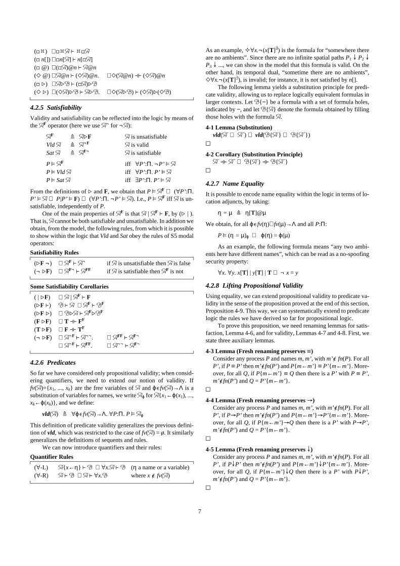
4.2.5 Satisfiability

Validity and satisfiability can be reflected into the logic by means ofthe $F�operator (here we use $¬ for ¬$):

From the definitions of ©�and F, we obtain that P � $F ⇔ (ÒP’ :Π.P’ � $ ⇒ P|P’ � F) ⇔ (ÒP’ :Π. ¬P’ � $). I.e., P � $F iff $�is un-satisfiable, independently of P.

One of the main properties of $F is that $ | $F L} F, by (©�| ).That is, $�cannot be both satisfiable and unsatisfiable. In addition weobtain, from the model, the following rules, from which it is possibleto show within the logic that Vld and Sat obey the rules of S5 modaloperators:

Satisfiabil ity Rules

Some Satisfiabil ity Corollar ies

4.2.6 Predicates

So far we have considered only propositional validity; when consid-ering quantifiers, we need to extend our notion of validity. Iffv($)={ x1, ..., xk} are the free variables of $ and ϕÐfv($)→Λ is asubstitution of variables for names, we write $ϕ�for ${ x1←ϕ(x1), ...,xk←ϕ(xk)} , and we define:

This definition of predicate validity generalizes the previous defini-tion of vld, which was restricted to the case of fv($) = Ô. It similarlygeneralizes the definitions of sequents and rules.

We can now introduce quantifiers and their rules:

Quantifier Rules

As an example, �Òx.¬(x[T]Ó) is the formula for “somewhere thereare no ambients” . Since there are no infinite spatial paths P1 � P2 �P3 � ..., we can show in the model that this formula is valid. On theother hand, its temporal dual, “sometime there are no ambients” ,2Òx.¬(x[T]Ó), is invalid; for instance, it is not satisfied by n[] .

The following lemma yields a substitution principle for predi-cate validity, allowing us to replace logically equivalent formulas inlarger contexts. Let %{ −} be a formula with a set of formula holes,indicated by −, and let %{$} denote the formula obtained by fill ingthose holes with the formula $.

4-1 Lemma (Substitution)vld($ª ⇔ $¨) ⇒ vld(%{$ª} ⇔ %{$¨} )

1

4-2 Corollary (Substitution Pr inciple)$ª�xML} $¨ ⇒ %{$ª} �xML} %{$¨}

1

4.2.7 Name Equality

It is possible to encode name equali ty within the logic in terms of lo-cation adjuncts, by taking:

We obtain, for all ϕÐfv(η)∪fv(µ)→Λ and all P:Π:

As an example, the following formula means “any two ambi-ents here have different names”, which can be read as a no-spoofingsecurity property:

4.2.8 Lifting Propositional Validity

Using equali ty, we can extend propositional validity to predicate va-lidity in the sense of the proposition proved at the end of this section,Proposition 4-9. This way, we can systematically extend to predicatelogic the rules we have derived so far for propositional logic.

To prove this proposition, we need renaming lemmas for satis-faction, Lemma 4-6, and for validity, Lemmas 4-7 and 4-8. First, westate three auxiliary lemmas.

4-3 Lemma (Fresh renaming preserves ��)Consider any process P and names m, m’ , with m’Ñ fn(P). For allP’ , if P � P’ then m’Ñfn(P’ ) and P{ m←m’ } � P’ { m←m’ } . More-over, for all Q, if P{ m←m’ } � Q then there is a P’ with P � P’ ,m’Ñfn(P’ ) and Q = P’ { m←m’ } .

1

4-4 Lemma (Fresh renaming preserves xyz)Consider any process P and names m, m’ , with m’Ñfn(P). For allP’ , if PxyzP’ then m’Ñfn(P’ ) and P{ m←m’ } xyzP’ { m←m’ } . More-over, for all Q, if P{ m←m’ } xyzQ then there is a P’ with PxyzP’ ,m’Ñfn(P’ ) and Q = P’ { m←m’ } .

1

4-5 Lemma (Fresh renaming preserves �)Consider any process P and names m, m’ , with m’Ñfn(P). For allP’ , if P�P’ then m’Ñfn(P’ ) and P{ m←m’ }�P’ { m←m’ } . More-over, for all Q, if P{ m←m’ }�Q then there is a P’ with P�P’ ,m’Ñfn(P’ ) and Q = P’ { m←m’ } .

1

(4�) 4�$ L} �4$(4 n[] ) 4n[$]�L} n[4$]( ������4�@) (4$)@n L} $@n( ������2�@) $@n L} (2$)@n. 2($@n) xML} (2$)@n

( ������4�©) $©% L} (4$)©%( ������2�©) (2$)©% L} $©%. 2($©%) L} (2$)©(2%)

$F $ $©FVld $ $ $¬F

Sat $ $ $F¬

$ is unsatisfiable$ is valid$ is satisfiable

P � $F

P � Vld $P � Sat $

iff ÒP’ :Π. ¬P’ � $iff ÒP’ :Π. P’ � $iff ÓP’ :Π. P’ � $

(©F ¬) $F L} $¬

(¬ ©F) $F¬ L} $FFif $ is unsatisfiable then $�is falseif $ is satisfiable then $F�is not

( | ©F) $ | $F L} F(©F�L}) %�L} $ $F�L} %F

(©F�©) %©$ L} $F©%F

(F ©F) T xML} FF

(T ©F) F xML} TF

(¬ ©F) $¬F L} $¬¬. $FF L} $F¬

$¬F L} $FF. $¬¬ L} $F¬

vld($) $ ÒϕÐfv($)→Λ. ÒP:Π. P � $ϕ

(Ò-L) ${ x←η} �L} % Òx.$�L} % (η a name or a variable)(Ò-R) $�L} % $�L} Òx.% where x Ñ�fv($)

η�= µ $ η[T]@µ

P � (η = µ)ϕ ⇔ ϕ(η) = ϕ(µ)

Òx. Òy. x[T] | y[T] | T ⇒ ¬ x = y

8

4-6 Lemma (Fresh renaming preserves �)For all closed formulas $, processes P, and names m, m’ , if m’Ñfn(P)∪fn($) then P � $ ⇔ P{ m←m’ } � ${ m←m’ } .

ProofThe proof is by induction on the number of symbols in the closedformula $. Note that the number of symbols in a formula is un-changed by substituting a name for a variable or another name. Con-sider an arbitrary process P, and any names m and m’ . If m=m’ thelemma holds trivially, so we may assume that m≠m’ . We show onlythe case for parallel composition and the case for universal quantifi-cation.

Case for |: We prove each half of the following separately, wherem’Ñfn(P)∪fn($ | %).

P � $ | % ⇔ P{ m←m’ } � ($ | %){ m←m’ } .

(⇒) Assume P � $ | %. We are to show that there are Q’ , Q” suchthat P{ m←m’ } � Q’ | Q” , Q’ � ${ m←m’ } , and Q” � %{ m←m’ } .By assumption, there are P’ , P” such that P � P’ | P” , P’ � $, andP” � %. Let Q’ = P’ { m←m’ } and Q” = P” { m←m’ } . By Lemma 4-3, P � P’ | P” and m’Ñfn(P) imply that m’Ñfn(P’ )∪fn(P” ) andP{ m←m’ } � Q’ | Q” . By induction hypothesis, m’Ñfn(P’ )∪fn($)and P’ � $ imply that Q’ � ${ m←m’ } , and also m’Ñfn(P” )∪fn(%)and P” � % imply that Q” � %{ m←m’ } .(⇐) Assume P{ m←m’ } � ($ | %){ m←m’ } . We are to show thatthere are P’ , P” such that P � P’ | P” , P’ � $, and P” � %. By as-sumption, there are Q’ , Q” such that P{ m←m’ } � Q’ | Q” , Q’ �${ m←m’ } , and Q” � %{ m←m’ } . By Lemma 4-3, P{ m←m’ } � Q’ |Q” and m’Ñfn(P) imply there is R with P � R, m’Ñfn(R) and Q’ | Q”= R{ m←m’ } , and hence that there are P’ , P” such that R = P’ | P” ,m’Ñfn(P’ ), m’Ñfn(P” ), Q’ = P’ { m←m’ } , and Q” = P” { m←m’ } . Byinduction hypothesis, m’Ñfn(P’ )∪fn($) and Q’ � ${ m←m’ } implythat P’ � $, and also m’Ñfn(P” )∪fn(%) and Q” � %{ m←m’ } implythat P” � %.

Case for Ò: We prove each direction of the following separately,where m’Ñfn(P)∪fn(Òx.$).

P � Òx.$ ⇔ P{ m←m’ } � (Òx.$){ m←m’ } .

(⇒) Assume P � Òx.$. Pick any name n. We are to show thatP{ m←m’ } � ${ m←m’ }{ x←n} . We spli t the proof into three cases.First, suppose that m=n. Pick a fresh name m” such that m” Ñ fn(P)∪fn($)∪{ m,m’ } . By assumption, P � ${ x←m” } . Since m’Ñfn(P)∪fn(${ x←m” } ), the induction hypothesis implies that P{ m←m’ } �${ x←m” }{ m←m’ } . Recall that m≠m’ . Then, since mÑfn(P{ m←m’ } ) and mÑfn(${ x←m” }{ m←m’ } ), we get that P{ m←m’ }{ m” ←m} � ${ x←m” }{ m←m’ }{ m” ←m} by a second applicationof the induction hypothesis. But because of the freshness of m” , wehave P{ m←m’ }{ m” ←m} = P{ m←m’ } and ${ x←m” }{ m←m’ }{ m” ←m} = ${ m←m’ }{ x←m} . Since m=n, we have shownP{ m←m’ } � ${ m←m’ } { x←n} .Second, suppose that m≠n and m’=n. By assumption, P � ${ x←m} .In general we know that m’Ñfn(P)∪fn($) and m≠m’ . Therefore, wecan apply the induction hypothesis to obtain P{ m←m’ } � ${ x←m}{ m←m’ } . We have ${ x←m}{ m←m’ } = ${ m←m’ } { x←m’ } . Sincem’=n, we have shown P{ m←m’ } � ${ m←m’ }{ x←n} .Third, suppose that m≠n and m’≠n. By assumption, P � ${ x←n} .We have that m’Ñfn(P)∪fn($) and in this case we know that m’≠n.Therefore, we can apply the induction hypothesis to obtainP{ m←m’ } � ${ x←n}{ m←m’ } . Since m≠n we have ${ x←n}{ m←m’ } = ${ m←m’ }{ x←n} . So we have shown P{ m←m’ } �${ m←m’ } { x←n} .

(⇐⇐) Assume P{ m←←m’ } �� (ÒÒx.$){ m←←m’ } . Pick any name n. Weare to show that P �� ${ x←←n} . We split the proof into three cases.First, suppose n=m’ . Pick a fresh name m” such that m” Ñfn(P)∪fn($)∪{ m,m’ } . By assumption, we have P{ m←m’ } � ${ m←m’ }{ x←m” } . We can calculate ${ m←m’ }{ x←m” } = ${ x←m” }{ m←m’ } since m≠m” . Then, since m’Ñfn(P)∪fn(${ x←m” } ), theinduction hypothesis implies P � ${ x←m” } . Again, since m’Ñfn(P)and m’Ñfn(${ x←m” } ), the induction hypothesis implies P{ m”←m’ } � ${ x←m” } { m” ←m’ } . But because of the freshness of m” ,this is P � ${ x←m’ } . Therefore, since n=m’ , we have shown P �${ x←n} .Second, take n≠m’ but n=m. By assumption, P{ m←m’ } �${ m←m’ } { x←m’ } . From m≠m’, we get ${ m←m’ }{ x←m’ } =${ x←m’ }{ m←m’ } . Moreover, we also get mÑfn(P{ m←m’ } ) andmÑfn(${ x←m’ } { m←m’ } . Hence, the induction hypothesis impliesP{ m←m’ }{ m’←m} � ${ x←m’ }{ m←m’ }{ m’←m} . Since m’Ñfn(P)∪fn($), we can calculate P{ m←m’ }{ m’←m} = P and${ x←m’ } { m←m’ }{ m’←m} = ${ x←m} . Therefore, we haveshown P ��${ x←n} .Third, suppose n≠m’ and n≠m. By assumption, P{ m←m’ } �${ m←m’ } { x←n} . Since n≠m we have ${ m←m’ }{ x←n} =${ x←n}{ m←m’ } . Since n≠m’ , m’Ñfn(P)∪fn(${ x←n} ). Hence, theinduction hypothesis implies P � ${ x←n} .1

4-7 Lemma (Fresh renaming preserves validity)If $�is closed and valid and m’Ñfn($) then ${ m←m’ } is closedand valid.

ProofWe can assume that m’≠m. Take any P and two distinct names n,n’Ñfn(P)∪fn($)∪{ m,m’ } . Since $ is valid we have, in particular, thatP{ m←n}{ m’←m} � $. By Lemma 4-6, since m’Ñfn(P{ m←n}{ m’←m} )∪fn($), we obtain P{ m←n}{ m’←m}{ m←m’ } � ${ m←m’ } . This is the same as P{ m←n} � ${ m←m’ } . Again by Lemma4-6, since mÑfn(P{ m←n} )∪fn(${ m←m’ } ), we obtain P{ m←n}{ n←m} � ${ m←m’ }{ n←m} . This is the same as P � ${ m←m’ } .Hence ${ m←m’ } is valid. Since $ is closed, so is ${ m←m’ } . 1

4-8 Lemma (Injective complete renaming preserves validity)If $ is closed and valid and ρÐfn($)→Λ is an injective renaming,then $ρ is closed and valid.

ProofLet ρ = { m1←n1, ..., mk←nk} , where { m1, ..., mk} = fn($) and all theni are distinct. Take fresh p1, ..., pk Ñ { m1, n1, ..., mk, nk} . By induc-tion on i ranging from 1 to k, since $ is closed and valid andpiÑfn(${ m1←p1} ...{ mi-1←pi-1} ), by using Lemma 4-7 at each step,we obtain that $ª�$�${ m1←p1} ...{ mk←pk} is closed and valid. Notethat fn($ª) = { p1, ..., pk} . Then again, by induction on i ranging from1 to k, since niÑfn($ª{ p1←n1} ...{ pi-1←ni-1} ), by using Lemma 4-7 ateach step, we obtain that $¨�$�$ª{ p1←n1} ...{ pk←nk} is closed andvalid. Since p1, ..., pk are fresh, $¨�= $ρ. 1

4-9 Proposition (L ift ing propositional validity)If $�is closed and valid, then for any injective map ψÐfn($)→ϑfrom names to variables, the formula (dfn($)⇒$)ψ is valid,where dfn($) is the conjunction of all inequalities ¬n=m suchthat n,m are distinct names in fn($).

9

ProofAssume that $�is closed and valid and that ψÐfn($)→ϑ is injective.By construction, we also have that dfn($)⇒$�is closed and valid.Take any ϕÐfv((dfn($)⇒$)ψ)→Λ (with rng(ψ)=dom(ϕ)) and con-sider ϕ�ψ. There are two cases. If ϕ is not injective then dfn($)ϕ�ψ isequivalent to F, and therefore (dfn($)⇒$)ϕ�ψ is valid. Otherwise, ifϕ is injective, then ϕ�ψ is also injective with dom(ϕ�ψ) = fn($) =fn(dfn($)⇒$). By Lemma 4-8, since dfn($)⇒$ is closed and valid,we have that (dfn($)⇒$)ϕ�ψ is closed and valid. We have shownthat ÒϕÐfv((dfn($)⇒$)ψ)→Λ. ÒP:Π. P � (dfn($)⇒$)ϕ�ψ; that is,vld((dfn($)⇒$)ψ).1

For example, the valid proposition: n[T] ⇒ ¬m[T] is trans-formed into the valid predicate ¬x=y ⇒ (x[T] ⇒ ¬y[T]). However,without the assumption ¬x=y, the predicate x[T] ⇒ ¬y[T] is not val-id: for predicate validity one must consider also the substitutions thatmap x and y to the same name.

4.2.9 Case Analysis Principle

When reasoning about equality, it is often convenient to reason bycases on whether the equality is true or false. To this end, we intro-duce a case analysis principle.

4-10 Definition (Classical Predicates)$ is classical i ff ÒϕÐfv($)→Λ. { P @�P � $ϕ} Ð {Π, Ô} .

1The predicates T, F, and η=µ are classical. So is the disjunction

and negation of classical predicates.

4-11 Proposition (Case Analysis Pr inciple)Let 6{ −} be a sequent with a set of formula holes, and $ be aclassical predicate. Then 6{ T} ∧ 6{ F} ⇒ 6{$} .

ProofTaking 6{ −} = %ª{ −} �L} %¨{ −} and %{ −} $ %ª{ −} ⇒ %¨{ −} , it issuff icient to show that vld(%{ T} ) ∧ vld(%{ F} ) ⇒ vld(%{$} ). As-sume vld(%{ T} ) ∧ vld(%{ F} ). Take any ϕÐfv(%{$} )→Λ and P:Π.By assumption we have P � %ϕ{ T} and P � %ϕ{ F} . Since $�is clas-sical, we have also that { Q @�Q � $ϕ} Ð {Π, Ô} . Consider the casewhere { Q @�Q � $ϕ} = Π so that for any P, P � $ϕ iff P � T. By Lem-ma 4-1, P � %ϕ{$ϕ} iff P � %ϕ{ T} , hence we obtain P � %ϕ{$ϕ} .Consider the case where { Q @�Q � $ϕ} = Ô so that for any P, P � $ϕiff P � F. By Lemma 4-1, P � %ϕ{$ϕ} iff P � %ϕ{ F} , hence we haveP � %ϕ{$ϕ} . In both cases, we have shown that ÒϕÐfv(%{$} )→Λ.ÒP:Π. P � %ϕ{$ϕ} , that is, vld(%{$} ).1

4.3 Logical Properties of Type Systems

In this section we briefly discuss applications of our logic to expressproperties guaranteed by type systems, beyond the standard state-ments of subject reduction. This section assumes knowledge of typesystems for the Ambient Calculus [5].

Consider the system of locking and mobili ty types for the Am-bient Calculus [5], recast for the calculus of this paper. The assump-tion p:Amb•[S] ensures that ambients named p are locked, that is,they cannot be dissolved by an open. We can prove that if E,p:Amb•[S], E’ �L} P : T, then P � 4(�(p[T]Ó) ⇒ 4�(p[T]Ó)). This ex-presses that in a well-typed process, once a locked ambient named psomewhere comes into being, ever after there wil l somewhere be anambient named p.

Moreover, the assumption q:Amb•[RS’ ] ensures that ambients

named q are locked and immobile, that is, they cannot be moved byin or out, nor dissolved by open. We can prove that if E,q:Amb•[RS’ ], E’ �L} P : T, then P � 4(q[T]Ó ⇒ 4q[T]Ó). This expressesthat in a well-typed process, once a locked, immobile ambient ap-pears at the top-level of the process, it will stay there ever after.Moreover, we can prove that if E, p:Amb•[S], q:Amb•[RS’ ], E’ �L} P :T, then P � 4(�(p[q[T]Ó]Ó) ⇒ 4�(p[q[T]Ó]Ó)). This expresses thatin a well-typed process, once a locked, immobile ambient named qis somewhere a child of a locked ambient named p, ever after therewill somewhere be a q child of p.

4.4 An Example

In this example we use the laws of 2, | , and ©, to analyze the con-sequences of composing two logical specifications.

The specifications describe two subsystems: a Shopper and aThief, and focus on what happens to the shopper’s wallet. The walletis described simply by the formula Wallet[T], leaving the contentsof the wallet unspecified. The absence of a wallet in a given locationis described by the formula NoWallet, defined as ¬(Wallet[T] | T),meaning that it is not possible to decompose the current location intoa part containing a wallet and some other part.

A thief is somebody who, in the direct presence of a wallet, canmake the wallet disappear. Its specification is Wallet[T] ©2NoWallet, and its implementation in the Ambient Calculus couldsimply be given by open Wallet.

A shopper is, initially, a person with a wallet (a Looker) who islater likely to become a Buyer. A buyer is a person who has pulledout the wallet, presumably to buy something. When a wallet hasbeen pulled out, it becomes vulnerable to a nearby thief.

In the following derivation, we show that the interaction of ashopper with a thief (possibly in some larger context) may result ina CrimeScene, which is a situation in which the shopper has no wal-let, and also there is no wallet to be found nearby.

We begin with the system Buyer | Thief; using the rules (©�| ) and (�|L}) we obtain:

Buyer | Thief = Person[NoWallet] | Wallet[T] | (Wallet[T] ©�2NoWallet)L} Person[NoWallet] | 2NoWallet

From the rules (2T) $�L}�2$, (Id), and (�| L}) we obtain, in general,$�| (2%)�L}�(2$)�| (2%). Then, by (2 | ) (2$) | (2%)�L} 2($ | %)and transitivity (derivable from (Cut)) we obtain $�| (2%)�L}�2($�|%). Using this fact in our example we obtain, by transitivity:

Buyer | Thief L}�2(Person[NoWallet]�| NoWallet) = 2CrimeScene

Using the rules (2�L}) $�L}�%� 2$�L}�2%, and (2�4) 22$�L}�2$,we derive:

2(Buyer | Thief) L}�22CrimeScene22CrimeScene L}�2CrimeScene

As before, we can derive (2$)�| %�L}�2($�| %); therefore:(2Buyer) | Thief L}�2(Buyer | Thief)

and, by transitivity from above:

NoWallet $ ¬(Wallet[T] | T)Looker $ Person[Wallet[T] | T]Buyer $ Person[NoWallet] | Wallet[T]Shopper $ Looker ∧ 2BuyerThief $ Wallet[T] ©�2NoWalletCrimeScene $ Person[NoWallet] | NoWallet

10

(2Buyer) | Thief L}�2CrimeScenethen, by weakening (W-L):

(Looker | Thief) ∧ ((2Buyer) | Thief) L}�2CrimeSceneNow let’s consider the system Shopper | Thief. By the distribution of| over ∧ (( | ∧), from section 4.2.2) we have:

Shopper | Thief = (Looker ∧ 2Buyer) | ThiefL} (Looker | Thief) ∧ ((2Buyer) | Thief)

and finally, by transitivity from above, we obtain:

5 A Decidable Sublogic

A model checker is an algorithm that determines the truth of an as-sertion P � $, given process P and formula $ as input. We describea model checker for the case where P is replication-free and $�is ©-free. The model checker depends on putting any replication-freeprocess into a normal form, given by a finite product of prime pro-cesses:

Products, Pr imes, and Normal Forms

The following recursive algorithm maps any replication-freeprocess to a list of prime processes representing a normal form struc-turally congruent to the original process. We write li sts of processesin the notation [P1, ..., Pk].

Normal Form for a Replication-Free Process

5-1 LemmaIf Norm(P) = [π1, ..., πk] then P ��ΠiÐ1..k πi.

1To check the sometime and somewhere modalities, we depend

on two routines Reachable and SubLocations that given a process Pcompute a representation of the sets of processes Q such that P xyyz*Q and P �* Q, respectively. We omit the straightforward definitionsof these routines. Instead, we state their desired properties, which areproved using techniques developed previously [12].

5-2 LemmaIf Reachable(P) = [P1, ..., Pk] then for all iÐ1..k, P xyyz* Pi, and forall Q, if P xyyz* Q then Q ��Pi for some iÐ1..k.

If SubLocations(P) = [P1, ..., Pk] then for all iÐ1..k, P �* Pi, andfor all Q, if P �* Q then Q ��Pi for some iÐ1..k.

1

Next, we define our model checking algorithm, and state itscorrectness property, Proposition 5-4, together with the main lem-mas used in its proof.

Checking Whether Process P Satisfies Closed Formula $

5-3 Lemmas(1) For all replication-free processes P and Q, and all replication-

free primes π1, ..., πk, P | Q ��ΠiÐ1..k πi if and only if there are setsI and J such that I∪J = 1..k, I∩J = Ô, P ��ΠiÐI πi, and Q ��ΠiÐJ πi.

(2) For all replication-free processes P, and all replication-freeprimes π1, ..., πk, n[P] ��ΠiÐ1..k πi if and only if k = 1 and there isQ with π1 = n[Q] and P � Q.

(3) For all replication-free processes P and ©-free closed formulasÒx.$, if { m1, ..., mk} = fn(P)∪fn($) and m0Ñ{ m1, ..., mk} , then: P� Òx.$ if and only if ÒiÐ0..k. P � ${ x←mi} .

1

5-4 PropositionFor all replication-free processes P and ©-free closed formulas $,P � $ if and only if Check(P, $) = T.

1Since all the recursive calls are on subformulas of the original

formula, the algorithm always terminates. When computingCheck(P, $ | %) with Norm(P) = [π1, ..., πk] there are 2k differentsubsets of 1..k, and so 2k different choices of the sets I and J. There-fore, in general the time complexity of Check(P, $) is at least expo-nential in the size of P. (The practical performance of this algorithmcan be greatly improved by special-casing and heuristics.)

Examples: define an n $ n[T]Ó, and p parents q $ p[q[T]Ó]Ó,and let P = a[p[out a. in b. jmk]] | b[open p. (x). x[]] , as in Section2.2. The algorithm returns the following results on various exampleformulas:

In summary, Proposition 5-4 shows that the model checkingproblem for the sublogic without © and the subcalculus without ! is

Shopper | Thief L}�2CrimeScene

ΠiÐ1..k Pi $ P1 | ... | Pk | 0π ::= M[P] @ n.P @ in M.P @ out M.P @ open M.P

@ (n).P @ jMkΠiÐ1..k πi

productprime process

normal form

Norm(0) $ []Norm(P | P’ ) $ [π1, ..., πk, π’1, ..., π’k’]

if Norm(P) = [π1, ..., πk] and Norm(P’ ) = [π’1, ..., π’ k’] Norm(M[P]) $ [M[P]]Norm(M.P) $ [M.P] if M Ð�{ n, in N, out N, open N}Norm(ε.P) $ Norm(P)Norm((M.N).P) $ Norm(M.(N.P))Norm((n).P) $ [(n).P]Norm(jMk) $ [jMk]

Check(P, T) $ TCheck(P, ¬$) $ ¬Check(P, $)Check(P, $ ∨ %) $ Check(P, $) ∨ Check(P, %)Check(P, 0) $ if Norm(P) = [] then T else FCheck(P, n[$]) $

if Norm(P) = [n[Q]] for some Q, then Check(Q, $), else FCheck(P, $ | %) $

let Norm(P) = [π1, ..., πk] in ÓI,J. I∪J=1..k ∧ I∩J=Ô ∧

Check(ΠiÐI πi, $) ∧ Check(ΠiÐJ πi, %)Check(P, Òx.$) $

let { m1, ..., mk} = fn(P)∪fn($) and m0Ñ{ m1, ..., mk} in ÒiÐ0..k. Check(P, ${ x←mi} )

Check(P, 2$) $ let [P1, ..., Pk] = Reachable(P) in ÓiÐ1..k. Check(Pi, $)

Check(P, �$) $ let [P1, ..., Pk] = SubLocations(P) in ÓiÐ1..k. Check(Pi, $)

Check(P, $@n) $ Check(n[P], $)

Check(P, an a) = TCheck(P, an b) = TCheck(P, an p) = FCheck(P, �an p) = T

Check(P, 2�an m) = TCheck(P, a parents p) = TCheck(P, b parents p) = FCheck(P, 2b parents p) = T

11

decidable. It is not clear in general how to extend this algorithm toinclude either ! or ©, because in principle an unbounded number ofprocesses needs to be considered. For example, checking the truth ofP � T©$ in principle requires showing for all processes P’ that P |P’ � $. Similarly, checking the truth of !P � ¬($ | T) in principlerequires showing that neither !P � $�nor Pk � $ for all k ≥ 0.

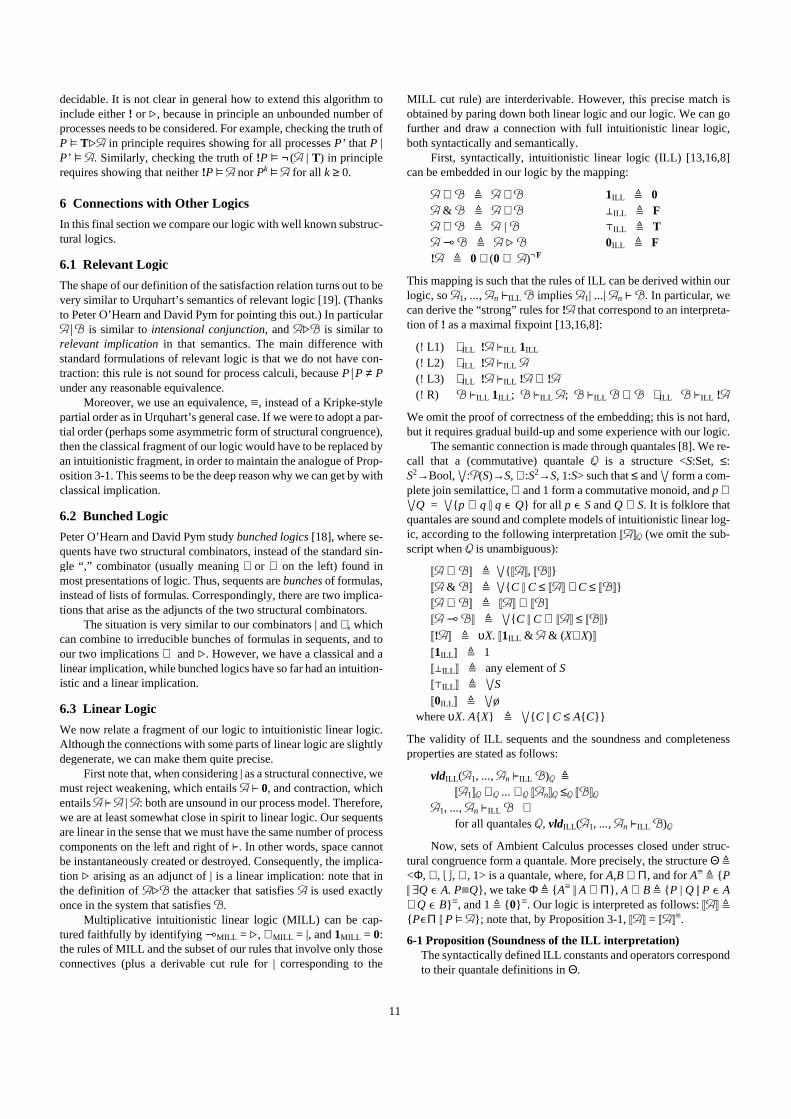
6 Connections with Other Logics

In this final section we compare our logic with well known substruc-tural logics.

6.1 Relevant Logic

The shape of our definition of the satisfaction relation turns out to bevery similar to Urquhart’s semantics of relevant logic [19]. (Thanksto Peter O’Hearn and David Pym for pointing this out.) In particular$_% is similar to intensional conjunction, and $©% is similar torelevant implication in that semantics. The main difference withstandard formulations of relevant logic is that we do not have con-traction: this rule is not sound for process calculi , because P_P ≠ Punder any reasonable equivalence.

Moreover, we use an equivalence, �, instead of a Kripke-stylepartial order as in Urquhart’s general case. If we were to adopt a par-tial order (perhaps some asymmetric form of structural congruence),then the classical fragment of our logic would have to be replaced byan intuitionistic fragment, in order to maintain the analogue of Prop-osition 3-1. This seems to be the deep reason why we can get by withclassical implication.

6.2 Bunched Logic

Peter O’Hearn and David Pym study bunched logics [18], where se-quents have two structural combinators, instead of the standard sin-gle “ ,” combinator (usually meaning ∧ or ⊗ on the left) found inmost presentations of logic. Thus, sequents are bunches of formulas,instead of lists of formulas. Correspondingly, there are two implica-tions that arise as the adjuncts of the two structural combinators.

The situation is very similar to our combinators | and ∧, whichcan combine to irreducible bunches of formulas in sequents, and toour two implications ⇒ and ©. However, we have a classical and alinear implication, while bunched logics have so far had an intuition-istic and a linear implication.

6.3 L inear Logic

We now relate a fragment of our logic to intuitionistic linear logic.Although the connections with some parts of linear logic are slightlydegenerate, we can make them quite precise.

First note that, when considering | as a structural connective, wemust reject weakening, which entails $ L} 0, and contraction, whichentails $ L} $ | $: both are unsound in our process model. Therefore,we are at least somewhat close in spirit to linear logic. Our sequentsare linear in the sense that we must have the same number of processcomponents on the left and right of L}. In other words, space cannotbe instantaneously created or destroyed. Consequently, the implica-tion © arising as an adjunct of | is a linear implication: note that inthe definition of $©% the attacker that satisfies $� is used exactlyonce in the system that satisfies %.

Multiplicative intuitionistic linear logic (MILL) can be cap-tured faithfully by identifying xyµMILL = ©, ⊗MILL = |, and 1MILL = 0:the rules of MILL and the subset of our rules that involve only thoseconnectives (plus a derivable cut rule for | corresponding to the

MILL cut rule) are interderivable. However, this precise match isobtained by paring down both linear logic and our logic. We can gofurther and draw a connection with full intuitionistic linear logic,both syntactically and semantically.

First, syntactically, intuitionistic linear logic (ILL) [13,16,8]can be embedded in our logic by the mapping:

This mapping is such that the rules of ILL can be derived within ourlogic, so $1, ..., $n LL}}ILL % implies $1| ...| $n LL}} %. In particular, wecan derive the “strong” rules for !$�that correspond to an interpreta-tion of ! as a maximal fixpoint [13,16,8]:

We omit the proof of correctness of the embedding; this is not hard,but it requires gradual build-up and some experience with our logic.

The semantic connection is made through quantales [8]. We re-call that a (commutative) quantale 4 is a structure <S:Set, ≤:S2→Bool, r:3(S)→S, ⊗:S2→S, 1:S> such that ≤ and r form a com-plete join semilattice, ⊗ and 1 form a commutative monoid, and p ⊗rQ = r{ p ⊗ q @ q Ð�Q} for all p Ð�S and Q ⊆ S. It is folklore thatquantales are sound and complete models of intuitionistic linear log-ic, according to the following interpretation ?$A4�(we omit the sub-script when 4�is unambiguous):

The validity of ILL sequents and the soundness and completenessproperties are stated as follows:

Now, sets of Ambient Calculus processes closed under struc-tural congruence form a quantale. More precisely, the structure Θ $<Φ, ⊆, t, ⊗, 1> is a quantale, where, for A,B ⊆ Π, and for A� $�{ P@ ÓQ Ð�A. P�Q} , we take Φ $�{ A� @ A ⊆ Π} , A ⊗ B $�{ P | Q @ P Ð�A∧ Q Ð�B} �, and 1 $�{ 0} �. Our logic is interpreted as follows: ?$A�${ PÐΠ @ P � $} ; note that, by Proposition 3-1, ?$A�= ?$A�.

6-1 Proposition (Soundness of the ILL interpretation)The syntactically defined ILL constants and operators correspondto their quantale definitions in Θ.

$ ⊕ %� $ $ ∨ %$ & %� $ $ ∧ %$ ⊗ %� $ $ | %$ xyµ %� $ $ © %!$� $ 0 ∧ (0 ⇒ $)¬F

1ILL� $ 0�ILL� $ F�ILL� $ T0ILL� $ F

(! L1) ILL !$ L}ILL 1ILL

(! L2) ILL !$ L}ILL $(! L3) ILL !$ L}ILL !$�⊗ !$(! R) % L}ILL 1ILL; % L}ILL $; % L}ILL %�⊗ % ILL % L}ILL !$

?$ ⊕ %A� $ r{ ?$A, ?%A}?$ & %A� $ r{ C @ C ≤ ?$A ∧ C ≤ ?%A}?$ ⊗ %A� $ ?$A ⊗ ?%A?$ xyµ %A� $ r{ C @ C ⊗ ?$A ≤ ?%A}

?!$A� $ υX. ?1ILL & $ & (X⊗X)A?1ILLA� $ 1?�ILLA� $ any element of S?�ILLA� $ rS

?0ILLA� $ rÔwhere υX. A{ X} � $ r{ C @ C ≤ A{ C} }

vldILL($1, ..., $n L}ILL %)4 $ ?$1A4 ⊗4 ... ⊗4 ?$nA4 ≤4 ?%A4

$1, ..., $n L}ILL % ⇔for all quantales4, vldILL($1, ..., $n L}ILL %)4

12

ProofWe detail the most interesting cases, for ⊗, xyµ, and !.

Case for ⊗: ?$ ⊗ %A = ?$A ⊗ ?%A.(P Ð ?$ ⊗ %A)�⇔�(P Ð ?$ | %A)�⇔�(P � $ | %)�⇔�(ÓP’ ,P” :Π. P �P’ | P” ∧ P’ � $ ∧ P” � %)�⇔�(P Ð { P’ | P” @ P’ � $ ∧ P” � %} ��)⇔�(P Ð { P’ | P” @ P’ Ð ?$A ∧ P” Ð ?%A} ��)�⇔�(P Ð ?$A ⊗ ?%A)

Case for xyµ: ?$ xyµ %A = ?$A xyµ ?%A.Let A = ?$A�and B = ?%A. (P Ð ?$A xyµ ?%A)�⇔�(P Ð A xyµ B)�⇔�(P Ðt{ C @ C ⊗ A ⊆ B} )�⇔�(ÓC. P Ð C ∧ C ⊗ A ⊆ B)�⇔�(ÓC. P Ð C ∧ÒQ. (ÓQ’,Q” . Q � Q’ | Q” ∧ Q’ Ð C ∧ Q” Ð A) ⇒ Q Ð B) ⇔ (ÒQ” .Q” Ð A ⇒ P | Q” Ð B). The last step is derived as follows:1) Assume ÓC. P Ð C ∧ ÒQ. (ÓQ’,Q” . Q � Q’ | Q” ∧ Q’ Ð C ∧ Q”Ð A) ⇒ Q Ð B. Take any R and assume R Ð A. Instantiate the assump-tion with P | R for Q and take Q’=P and Q” =R; we obtain P | R Ð B. 2) Conversely, assume ÒR. R Ð A ⇒ P | R Ð B. Take C={ P} �, takeany Q, and assume (ÓQ’,Q” . Q � Q’ | Q” ∧ Q’ Ð { P} � ∧ Q” Ð A).Instantiating the assumption with Q” for R, we obtain P | Q” Ð B.Now, Q’ ��P by assumption, hence P | Q” ��Q’ | Q” � Q. Since Bis �-closed, we obtain Q Ð B.Hence, (P Ð ?$A xyµ ?%A) ⇔ (ÒQ” . Q” Ð A ⇒ P | Q” Ð B) ⇔ (ÒQ” .Q” � $ ⇒ P | Q” � %) ⇔ (P � $ © %) ⇔ (P Ð ?$ © %A) ⇔ (P Ð?$ xyµ %A).

Case for !: ?!$A = !?$A.First we show that ÒP. 0 � $ ⇔ P � (0 ⇒ $)¬F. Take any P; by definition of ©, we have P � (0 ⇒ $)¬F ⇔ (ÒQ. Q� 0 ⇒ $). Then, (ÒQ. Q � 0 ⇒ $) ⇔ (ÒQ. Q � 0 ⇒ Q � $) ⇔ 0� $. The last step is by instantiation of Q with 0, in one direction,and by Proposition 3-1, in the other direction.Then we compute: (P Ð ?!$A) ⇔ (P Ð ?0 ∧ (0 ⇒ $)¬FA) ⇔ (P � 0 ∧P � (0 ⇒ $)¬F) ⇔ (P � 0 ∧ 0 � $).Now, in a quantale !A = υX. 1 & A & (X⊗X), which in Θ means υX.{ 0} � ∩ A ∩ (X | X). If 0 Ñ A then {0} � ∩ A = Ô, and !A = Ô. If instead0 Ð A, then {0} � ∩ A = { 0} �, and !A = υX. { 0} � ∩ (X | X). We havethat { 0} � is a fixpoint of λX. { 0} � ∩ (X | X); moreover, if B = { 0} �

∩ (B | B) then B ⊆ {0} �, hence { 0}� is the greatest fixpoint, and !A= { 0} �. In conclusion: if 0 Ñ A then !A = Ô�else if 0 Ð A then !A ={ 0} � and, by contrapositive, if !A ≠ Ô then 0 Ð A.Hence P Ð !?$A �⇒ !?$A ≠ Ô ⇒ 0 Ð ?$A ⇒ !?$A = { 0}� ⇒ P Ð{ 0} �; that is P Ð !?$A ⇒ P � 0 ∧ 0 � $. Conversely, if P � 0 ∧ 0 �$, then 0 Ð ?$A ⇒ !?$A = { 0} � ⇒ P Ð !?$A.In conclusion P Ð !?$A �⇔ �P � 0 ∧ 0 � $ �⇔ �P Ð ?!$A.1

Moreover, in our model the linear notion of validity matchesour notion of validity:

6-2 PropositionLet $1, ..., $n, % be formulas in ILL.

vldILL($1, ..., $n L}ILL %)Θ� ⇔ vld($1 | ... | $n L} %)

(For n=0 this means: vldILL(�L}ILL %)Θ� ⇔ vld(0 L} %).)

Proof(ÒP. P � $1 | ... | $n ⇒ %) ⇔ (ÒP. P � $1 | ... | $n ⇒ P � %)⇔ (ÒP. P Ð ?$1 | ... | $nA ⇒ P Ð ?%A) ⇔ ?$1 | ... | $nA ⊆ ?%A⇔ ?$1A ⊗ ... ⊗ ?$nA ⊆ ?%A. The last step is as in the ⊗ case of Proposition 6-1.1

The discrepancies with ILL are as follows. We identify �ILL

and 0ILL (as F); therefore, $� acquires special properties. The addi-tives ⊕ and & distribute over each other (both semantically and as a

derived rule). The semantic interpretation of !$ is rather degenerate;in particular, !$ xyµ %�does not seem to have an interesting meaning.

Conclusions and Fur ther Work

We have introduced an expressive logic that can describe propertiesof spatial configurations and of mobile computation, including secu-rity properties. Although some attack scenarios can already be de-scribed, many interesting security properties require the use of namerestriction (which is already present in our full Ambient Calculus):we intend to study extensions of our logic in that direction. We alsointend to study recursive modal formulas. Finally, we should consid-er issues of logical completeness: these have not been looked at be-cause our focus has been on studying properties of the model. Theonly sense in which we feel we have a “large enough” set of rules isthat we can logically derive the rules of intuitionistic linear logic.

We have previously developed type systems for mobility; nowwe have a model-checking algorithm for a decidable sublogic, and amore complete logic of mobility. These can be seen as three progres-sive stages in the screening of mobile code, corresponding to byte-code verification by type checking, by model checking, and by proofchecking (as in proof-carrying code). In all these cases, it is possibleto express and verify properties of mobile code that allow the codeto move around after verification, safely removing the constraints ofrigid sandboxing policies.

Acknowledgments

Giorgio Ghelli participated in the initial discussions leading to thislogic. Barney Hilken and Peter O’Hearn both pointed out that ‘©’ �isadjunct to ‘ |’ . Glynn Winskel directed us to the connection with in-tuitionistic linear logic. Peter O’Hearn and David Pym pointed us toliterature on relevant logic. Gordon Plotkin suggested the new axi-oms for structural congruence. Useful comments were made byMartín Abadi and Todd Knoblock.

References

[1] Abadi, M., Plotkin, G.D.: A Logical View of Composition.TCS 114(1), 3-30, 1993.

[2] Amadio, R.M., Prasad, S.: Localities and failures. FST &TCS '94, LNCS 880, 205-216, Springer, 1994.

[3] Cardelli , L., Gordon, A.D.: Mobile Ambients. FoSSaCS’98,LNCS 1378, 140-155, Springer, 1998.

[4] Cardelli , L., Gordon, A.D.: Types for M obile Ambients.POPL’99, 79-92, 1999.

[5] Cardelli , L., Ghell i, G., Gordon, A.D.: Mobility Types forMobile Ambients. ICALP’99. LNCS 1644, 230-239, Spring-er, 1999.

[6] Dam, M.: Relevance Logic and Concurr ent Composition.LICS’88, 178-185, 1988.

[7] Došen, K.: A Histor ical Introduction to Substructural Log-ics. In: Schroeder-Heistler, P., Došen, K. (eds.): SubstructuralLogics. Studies in Logic and Computation 2, 1-30, ClarendonPress, 1994.

[8] Engberg, U.H., Winskel, G.: Linear Logic on Petr i Nets.BRICS Report RS-94-3, 1994.

[9] Engelfriet, J.: A Multiset Semantics for the π-calculus withReplication. TCS 153, 65-94, 1996.

13

[10] Fournet, C., Gonthier, G.: A Calculus of Mobile Agents.CONCUR’96, LNCS 1119, Springer, 1999.

[11] Gentzen, G.: Untersuchungen über das logische Schließen.Mathematische Zeitschrift 39, 176-210, 405-431, 1935. En-glish translation in: The collected papers of Gerhard Gentzen.M.E.Szabo (ed.), 132-213, North Holland, 1969.

[12] Gordon, A.D., Cardell i, L.: Equational Properties of MobileAmbients. FoSSaCS’99, LNCS 1578, 212-226, Springer,1996.

[13] Girard, J.-Y., Lafont, Y.: Linear Logic and Lazy Computa-tion. TAPSOFT 87, LNCS 250 vol 2, 53-66, Springer, 1987.

[14] Girard, J.-Y., Lafont, Y., Taylor, P.: Proofs and Types. Cam-bridge University Press, 1989.

[15] Hennessy, H., Milner, R.: Algebraic Laws for Nondetermin-ism and Concurrency. JACM, 32(1)137-161, 1985.

[16] Lafont, Y.: The L inear Abstract Machine. TCS (59)157-180, 1988.

[17] Milner, R.: Flowgraphs and Flow Algebras. JACM 26(4),1979.

[18] O’Hearn, P.W., Pym, D.: The Logic of Bunched Implica-tions. Bulletin of Symbolic Logic. To appear, 1999.

[19] Urquhart, A.: Semantics for Relevant Logics. Journal ofSymbolic Logic 37(1)159-169, 1972.

[20] Vitek, J., Castagna, G.: Seal: A Framework for Secure Mo-bile Computations. Internet Programming Languages, LNCS1686, 47-77, Springer, 1999.

Appendix: Rules of the Ambient Logic

This appendix collects information already presented in the paper.

Sequents: $�L} %Rules: $1�L} %1; ...; $n�L} %n� $�L} % (n≥0)

Abbreviations: xML}�means L}�in both directions; means �in bothdirections.

Propositional Rules

(A-L) $∧(&∧')�L} % ($∧&)∧'�L} %(A-R) $�L} (&∨')∨% $�L} &∨('∨%)(X-L) $∧&�L} % &∧$�L} %(X-R) $�L} &∨% $�L} %∨&(C-L) $∧$�L} % $�L} %(C-R) $�L} %∨% $�L} %(W-L) $�L} % $∧&�L} %(W-R) $�L} % $�L} &∨%(Id) $�L} $(Cut) $�L} &∨%; $ª∧&�L} %ª $∧$ª�L} %∨%ª

(T) $∧T�L} % $ L} %(F) $�L} F∨% $ L} %(¬-L) $�L} &∨% $∧¬&�L} %(¬-R) $∧&�L} % $�L} ¬&∨%

Quantifier Rules

(Ò-L) ${ x←η} �L} % Òx.$�L} % (η is a name or a variable)(Ò-R) $�L} % $�L} Òx.% where x Ñ�fv($)

Composition Rules

( | 0) $ | 0 xML} $( | ¬0) $ | ¬0 L} ¬0(A | ) $ | (% | &) xML} ($ | %) | &(X | ) $ | % L} % | $( | L}) $ª�L} %ª; $¨�L} %¨ $ª | $¨ L} %ª | %¨

( | ∨) ($∨%) | & L} $ | &�∨ % | &( | || ) $ª | $¨ L} ($ª | %¨)�∨ (%ª | $¨)�∨ (¬%ª | ¬%¨)

( | ©) $ | &�L} % $�L} &©%(©F ¬) $F L} $¬

(¬ ©F) $F¬ L} $FF

Location Rules

(n[] �¬0) n[$]�L} ¬0(n[] �¬ | ) n[$]�L} ¬(¬0 | ¬0)(n[] �L}) $�L} % n[$]�L} n[%](n[] ∧) n[$]∧n[%]�L} n[$∧%](n[] ∨) n[$∨%] L} n[$]∨n[%]

(n[] @) n[$]�L} % $�L} %@n(¬ @) $@n�xML} ¬((¬$)@n)

Time and Space Modality Rules

(2) 2$ xML} ¬4¬$

(4 K) 4($ ⇒ %) L} 4$ ⇒ 4%(4 T) 4$ L} $(4 4) 4$ L} 44$(4 T) T L} 4T(4 L}) $�L} % 4$�L} 4%

(�) �$ xML} ¬�¬$

(� K) �($ ⇒ %) L} �$ ⇒ �%

(� T) �$ L} $(� 4) �$ L} ��$

(� T) T L} �T(� L}) $�L} % �$�L} �%

(2 n[]) n[2$]�L} 2n[$](2 | ) 2$ | 2%�L} 2($ | %)

(� n[]) n[�$]�L} �$

(� | ) �$ | %�L} �($ | T)

(�2) �2$ L} 2�$