1

This is an electronic version of an article published in Georisk, Vol. 5, No. 1, March 2011, p 44-58 The typeset article is available online at: http://www.informaworld.com/10.1080/17499511003679931

Uncertainty treatment in earthquake modeling using Bayesian probabilistic networks

Yahya Y. Bayraktarli Institute of Structural Engineering, Group Risk and Safety, ETH Zurich HIL E22.2, Wolfgang-Pauli-Str. 15, CH-8093 Zurich Jack W. Baker Department of Civil and Environmental Engineering, Stanford University Yang & Yamasaki Energy & Environment Building, Room 283, Stanford, CA 94305-4020, Michael H. Faber Institute of Structural Engineering, Group Risk and Safety, ETH Zurich HIL E23.3, Wolfgang-Pauli-Str. 15, CH-8093 Zurich

Abstract A probabilistic description of potential ground motion intensity is computed using a Bayesian Probabilistic Network (BPN) representing the standard probabilistic seismic hazard analysis (PSHA). Two earthquake ground motion intensity parameters are used: response spectral values for structural failures and peak ground acceleration for geotechnical failures. The correlation of these parameters is also considered within a BPN. It is further shown how deaggregation of the seismic hazard could be easily performed using BPN’s. A systematic consideration of uncertainty in the values of the parameters of a particular seismic hazard model can be described by PSHA. But the correct choices for elements of the seismic hazard model are uncertain. Logic trees provide a convenient framework for the treatment of model uncertainty. The paper illustrates an alternative way of incorporating the model uncertainty by extending the developed BPN. Incorporation of time-dependant seismic hazard using a BPN is also illustrated. Finally, the uncertainty treatment in earthquake modeling using BPN’s is illustrated on the region Adapazari, which is located close to the western part of the North Anatolian Fault in Turkey. 1. Introduction State-of-the-art seismic hazard studies calculate the probability of occurrence of a ground motion intensity parameter within a given time period due to an earthquake using earth science models for the characteristics of earthquakes in the region of interest. Uncertainty about the causes and effects of earthquakes and about the seismic characteristics of potential active faults lead to uncertainties in the input parameters for the seismic hazard analysis. Cornell (1968) proposed a mathematical approach for systematically incorporating the uncertainties for calculating probability of exceeding some level of earthquake ground shaking at a site. The methodology is known as Probabilistic Seismic Hazard Analysis (PSHA) and comprises in summary four steps: • Identification of all earthquake sources capable of producing ground motions, specifying the

uncertainty in location.

2

• Characterization of the temporal distribution of earthquake recurrence, specifying the uncertainty in magnitude and time of occurrence.

• Prediction of the resulting ground motion intensity as a function of location and magnitude. • Combination of the uncertainties in location, magnitude, time and ground motion intensity,

using the total probability theorem. In more advanced seismic hazard studies two types of uncertainty, namely aleatory variability and epistemic uncertainty, are distinguished. The uncertainty in size, location and time of the next earthquake and the resulting ground motion are considered to be inherent to the natural physical process and indifferent to change in our knowledge. Hence they are called aleatory variability or sometimes also randomness. Epistemic uncertainty results from our imperfect knowledge about earthquakes and can be reduced with a better knowledge basis and additional data (NRC 1997). The combination of the aleatory variability in location, size and time and ground motion intensity yields a single hazard curve (i.e., a curve reporting annual rates of exceedance for varying levels of ground motion intensity). Considering different assumptions, hypotheses, models or parameter values for the location, size and time to the next earthquake and for the predicted ground motion yields a suite of hazard curves representing the epistemic uncertainty. These epistemic uncertainties are typically organized and displayed by means of logic trees (Kulkarni et al., 1985; Coppersmith and Youngs 1985). Quantification and treatment of these epistemic uncertainties is carefully considered in the SSHAC Level 4 methodology, where a systematic and well-balanced integration of experts was a central issue (NRC 1997; Stepp et al. 2001; Abrahamson et al. 2001). In this paper the application of the state-of-the-art PSHA methodology using Bayesian Probabilistic Networks (BPN) is considered. After illustrating a generic application, aspects regarding the correlation of several ground motion intensity measures, incorporation of epistemic uncertainties and non-Poisson earthquake recurrence are discussed. In traditional PSHA studies, the primary analysis output is the annual frequency of exceeding some level of earthquake ground shaking at a site. In contrast, the main output of the BPN based seismic hazard calculation is the probability distribution of the maximum ground motion intensity measures observed in some window of time. The two output formats have a one-to-one relationship, so this transformation from one to the other is introduced because of the needfor these distributions in a newly developed generic indicator-based risk assessment framework based on BPN’s, which is illustrated in an accompanying paper (Bayraktarli and Faber 2008). 2. Bayesian probabilistic networks BPN’s constitute a flexible, intuitive and strong model framework for Bayesian probabilistic analysis (Jensen 2001). BPN’s may replace both fault and event trees and can be used at any stage of a probabilistic analysis. Due to their mind mapping characteristic, they comprise a significant support in the early phases of a probabilistic analysis, where the main task is to identify the potential scenarios and the interrelation of events leading to adverse events. N is a Bayesian network triplet ( , , )V A P , where:

• V is a set of variables , 1,2,3...iv i .

• A is a set of links showing causal interrelations between variables. A and V form a directed acyclic graph.

• ( | ) : vP P v v V , where v is the set of parents of v . In words P is the set the

conditional probabilities of the all variables given their parents.

3

It is common to visualize the variables in a BPN as nodes. A BPN may be formulated by the following steps, see also Figure 1: • Variables necessary and sufficient to model the problem framework of interest are identified. • Causal interrelations existing between the nodes are formulated, graphically shown by arrows. • A number of discrete mutually exclusive states are assigned to each variable. • Probability tables are assigned for the states of each of the variables. More formally, the BPN maps the joint probability distribution, ( )NP V , of a considered system.

( ) ( | )

N vv V

P V P v (1)

As an example, for the principle BPN in Figure 1 the joint probability is given by:

( , , ) ( ) ( ) ( | , )NP A B C P A P B P C A B (2) The marginal probability of any variable, say variable C in Figure 1, is defined by marginalizing all variables different from variable C out of the joint probability:

/

( ) ( ) N NV C

P C P V (3)

There may be evidence that some of the variables have specific values. For example, the variable B in the BPN in Figure 1 may be observed to be in State I. Then the posterior probability of any variable in the BPN, for example of variable C is defined as:

( , State I)( | State I)

( State I)

N

NN

P C BP C B

P B (4)

Efficient so-called inference engines are available for the numerical evaluation of Equations (2)-(4) (Jensen 2001). The computations in this paper are performed with the commercial software Hugin Researcher (2008).

4

Figure 1. A sample Bayesian Probabilistic Network.

A Bayesian Probabilistic Network for a generic seismic source The application of the BPN approach for seismic hazard analysis is described using a generic line source as specified in Kramer (1996). Line sources are tectonic faults capable of producing earthquakes of different sizes. In case when individual faults cannot be identified, the earthquake sources may be described by areal zones. The application of the approach to areal sources is analogous to the herein described line source. To predict the ground shaking at a site, the distribution of distances from the earthquake epicenter to the site of interest is necessary. The seismic sources are defined by epicenteres assumed to have equal probability. In a line sources these equal probability locations fall along a line; in a point source they would fall on a single point; in other cases areal sources are postulated. Using the geometric characteristics of the source, the distribution of distances can be calculated easily (Figure 2, left). Gutenberg and Richter (1944) observed that the distribution of earthquake magnitudes in a region generally follows a distribution given by log m a bM (5) where m is the rate of earthquakes with magnitude greater than m, and a and b are constants. a and b are generally estimated using statistical analysis of historical observations. a indicates the overall rate of earthquakes in a region, and b the relative ration of small to large magnitudes. The above described Gutenberg-Richter recurrence law is sometimes applied with a lower and upper bound. The lower bound is represented by a minimum magnitude mmin below which earthquakes are ignored due to their lack of engineering importance. The upper bound is given

5

Figure 2. Specification of the generic line source and discrete probabilities of distance (a, b), Gutenberg-Richter recurrence law and discrete probabilities of magnitude (c, d), and probability distribution of epsilon

and discrete probabilities for 50 states (e, f).

by the maximum magnitude mmax that a given seismic source can produce. Setting a range of magnitudes of interest, using the bounds Lm and Um , Equation 6 can be used to compute the probability that an earthquake magnitude falls within these bounds (Figure 2, middle).

|

L U

min max

M U M L L U min max

m m

m m

F m F m P m M m m M m

(6)

The earthquakes are modelled by ground motion prediction equations, which predict the probability distribution of ground motion intensity, as a function of many variables such as the earthquake’s magnitude, source-to-site distance, faulting mechanism, near surface site condition, etc. Ground motion prediction equations, also called attenuation functions, are generally developed using statistical analysis of measurements from past earthquakes. As there is significant scatter in the measured ground motion intensities, the ground motion prediction equation provides a probability distribution for the intensity parameter. Generally the predictive equations specify the predicted mean and the standard deviation of the intensity measure. The distribution of the ground motion intensity measure is then calculated by adding a normalized residual to the predicted mean. This factor is often denoted epsilon, . A BPN for the generic line source is constructed by conditioning the ground motion intensity parameter (here spectral displacement (SD)) on magnitude, M distance, R and epsilon, . Equation 6 is used to calculate the probabilistic distribution of magnitudes into 10 bins of equal intervals. Using simple geometric considerations, the distribution of the distance of the site to the generic line source is calculated also for 10 bins. The distribution of epsilon is discretized into 50 bins. The spectral displacement node is discretized also into 10 bins. For any of the combinations

6

of the 10 magnitudes, 10 distances and 50 epsilons the corresponding spectral displacement values are calculated using the ground motion prediction equation (Boore et al. 1997). The vector with the size of the number of bins for the spectral displacement has an entry of unity in the bin, where the ground motion intensity value falls. The 5000 vectors (multiplying 10x10x50) form the conditional probability table of spectral displacement. Having constructed the structure of the BPN and the corresponding probability tables, the BPN can be evaluated to yield the marginal distributions for any parameter in the network. These probability distributions may now be used to calculate the joint distribution of all or any set of the parameters in the network using simple probabilistic calculation schemes. In Figure 3 the BPN for seismic hazard analysis of the generic line source is illustrated with the marginal distribution of the spectral displacement. Once constructed, the BPN can be used to find the conditional distribution of any parameter, given knowledge of the state of any other parameter in the BPN. In Figure 3 the distribution of the spectral displacement is given for the situation that the magnitude is known to be 5.5 and the distance to be 60 km.

Figure 3. BPN for a generic seismic line source (a), discrete probabilities of SD (T=0.49 s) evaluated using the BPN for the probability distributions given in Figure 2 (b, c).

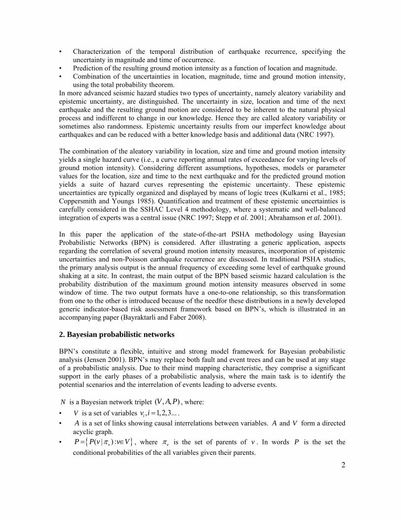
The information about which earthquake scenarios are most likely to produce a specific level of ground motion intensity can be retrieved from a PSHA computation through a process known as deaggregation (McGuire 1995). Using the constructed BPN and by instantiating, i.e. by assigning certainty to any state of any node, the conditional probabilities of the other nodes or the joint probability of any node combination can easily be retrieved. A sample deaggregation result for the magnitude - distance deaggregation given a SD (T=0.49 s) of between 4 mm and 5 mm is given in Figure 4. To verify the constructed BPN, the same magnitude-distance deaggregation is computed using a traditional PSHA analysis procedure (Figure 4). The small discrepancies in the probabilities arise from differences in the discretisation schemes between the traditional PSHA analysis and the BPN.

7

Figure 4. Deaggregation by magnitude and distance for SD= 4.4 mm using traditional PSHA (left), and for

4 mm<=SD<5 mm using BPN (right).

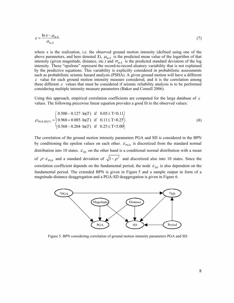
4. Incorporation of the Correlation of Ground motion intensity parameters By combining probabilistic descriptions of ground motion intensity with predictions of structural or geotechnical response as a function of that intensity, it is possible to compute the seismic reliability of engineering systems. This approach has been used for assessment of structural reliability (Bazzurro and Cornell 1994; Cornell et al. 2000) as well as geotechnical reliability considering liquefaction failures (Kramer et al. 2006). But reliability assessments that attempt to simultaneously consider both structural and geotechnical failures are currently not possible using this approach, because structural and geotechnical responses are generally predicted using different ground motion intensity parameters, and the tools are not available for determining a probabilistic characterization of the joint occurrence of these parameters (Baker 2007). Structural response (and structural failure) is often predicted using elastic spectral displacement (SD) (Pinto et al. 2004). Liquefaction failure, on the other hand, is typically predicted using peak ground acceleration (PGA) (Cetin et al. 2004; Youd et al. 2001). In this section, the correlation coefficient models necessary to achieve the goal of considering both structural and liquefaction failures simultaneously are developed based on Baker (2007). The needed correlation coefficients are obtained by first selecting a large set of recorded ground motions. Ground motion intensity parameters are then computed for each ground motion, along with predicted values for these parameters provided by ground motion prediction models. Correlations among the prediction residuals of the ground motion intensity parameters are then computed, and simple analytic equations are fitted to provide a simple means of calculating the required correlation coefficients. All of these intensity parameters are well represented by lognormal distributions, conditional upon earthquake magnitude, distance, and other parameters. Mean values and standard deviations for the possible values that the logarithms of these parameters may take in a given earthquake scenario are given by ground motion prediction models. The prediction model of Abrahamson and Silva (1997) is used for the SD and the model of Boore et al. (1997) for the PGA. Once these models are used to compute means and standard deviations of the intensity for a given ground motion, one can compute a normalized residual, that indicates the number of standard deviations away from the mean prediction a given observation is, using the following equation:

8

ln

ln

ln X

X

x

(7)

where x is the realization, i.e. the observed ground motion intensity (defined using one of the above parameters, and here denoted X), ln X is the predicted mean value of the logarithm of that intensity (given magnitude, distance, etc.) and ln X is the predicted standard deviation of the log intensity. These “epsilons” represent the record-to-record aleatory variability that is not explained by the predictive equations. This variability is explicitly considered in probabilistic assessments such as probabilistic seismic hazard analysis (PSHA). A given ground motion will have a different value for each ground motion intensity measure considered, and it is the correlation among these different values that must be considered if seismic reliability analysis is to be performed considering multiple intensity measure parameters (Baker and Cornell 2006). Using this approach, empirical correlation coefficients are computed for the large database of values. The following piecewise linear equation provides a good fit to the observed values:

, ( )

0.500 0.127 ln( ) if 0.05 T<0.11

0.968 0.085 ln( ) if 0.11 T<0.25

0.568 0.204 ln( ) if 0.25 T<5.00PGA SD T

T

T

T

(8)

The correlation of the ground motion intensity parameters PGA and SD is considered in the BPN by conditioning the epsilon values on each other. PGA is discretized from the standard normal

distribution into 10 states. SD on the other hand is a conditional normal distribution with a mean

of PGA and a standard deviation of 21 and discretized also into 10 states. Since the

correlation coefficient depends on the fundamental period, the node SD is also dependent on the

fundamental period. The extended BPN is given in Figure 5 and a sample output in form of a magnitude-distance deaggregation and a PGA-SD deaggregation is given in Figure 6.

Figure 5. BPN considering correlation of ground motion intensity parameters PGA and SD.

9

Figure 6. Deaggregation by magnitude and distance using BPN for PGA=0.05g, SD=3mm (left) and by PGA

and SD for M=6.8, R=27km (right).

5. Incorporating Model uncertainties For one particular seismic hazard model (defined by specifying a source model, a recurrence model and a ground motion prediction model) the aleatory variability described by that model is systematically considered. But there is still an uncertainty about the best choices for elements of the seismic hazard model itself. This is now commonly addressed by combining the uncertainties about the various inputs in logic trees (Kulkarni et al. 1984; Coppersmith and Youngs, 1986; SSHAC 1997). Each branch of a logic tree represents a set of chosen elements for a seismic hazard model. For each of the seismic hazard models the hazard calculations are performed and a single hazard curve representing ground motion versus annual frequency of exceedance is produced. The relative weighting of each hazard curve is then determined by multiplying the weights in each of the branches. From this set of hazard curves a mean, a median and curves for different fractiles can be defined. The BPN for the seismic hazard model introduced before will now be extended to incorporate model uncertainties. For each of the elements producing branches in a logic tree, a node is introduced into the network and the required dependencies with the existing nodes are set using additional arrows. The simple logic tree shown in Figure 7 allows uncertainty in selection of models for ground motion prediction equations and maximum magnitude to be considered. The ground motion prediction equations of Boore et al. (1997) and Abrahamson and Silva (1997) are considered, assigning weights of 0.7 and 0.3 respectively. At the other level of nodes, weights of 0.4 and 0.6 are assigned to the maximum magnitudes Mw=7.3 and Mw=7.7 the single line source is capable of producing. A sample output of the BPN in Figure 7 is given in Figure 8.

10

.

Figure 7. Logic tree and corresponding BPN considering modeling uncertainties.

Figure 8. Contribution by ground motion prediction equation and maximum magnitude choice for

PGA=0.15g, SD=6mm (left) and for PGA=0.25g, SD=5mm (right).

6. Incorporating time-dependant seismic hazard Earthquake occurrences are stochastic in nature, both in time and space. Small and medium magnitude earthquakes may occur independently implying a Poisson model. Large magnitude earthquakes on a particular fault segment, however, should not be independent from each other according to the elastic rebound theory (Reid 1911). As earthquakes occur to release the stress accumulation in a fault, the occurrence of a large earthquake should reduce the chances for occurrence of a following independent large earthquake in the same source. Paleoseismic studies on fault slip data led to the ‘characteristic earthquake’ recurrence model (Kramer, 1996). The seismic sources tend to generate regularly earthquakes of similar sizes near to the maximum magnitude known as characteristic earthquakes. This tendency is not seen for smaller earthquakes, which occur more or less randomly. Hence the earthquakes are classified into two groups; small/ medium size earthquakes and characteristic earthquakes. For small and medium size earthquakes a time-independent recurrence model and for characteristic earthquakes a time-dependent recurrence model is assumed. A review of non-Poisson models is presented in Anagnos and Kiremidjian (1988). The application of BPN’s for non-Poisson recurrence models is illustrated using the Brownian Passage Time (BPT) model developed by Matthews et al. (2002) and used in Takahashi et al. (2004). The occurrence of earthquakes of magnitude M constitutes a renewal process with ( , )Tf t M denoting the probability density function (PDF) of the interarrival times. Such a process reduces to the Poisson process, if ( , )Tf t M is taken as an exponential distribution. For all non-characteristic

11

earthquakes in the source a Poisson model and for the characteristic earthquake a more generalized renewal model is assumed. Setting the origin of time to the most recent occurrence of the characteristic earthquake and denoting the waiting time to the n-th occurrence of the characteristic event by nW , the conditional PDF of the waiting time to the n-th characteristic event, given that no characteristic earthquake has happened before the start of the operating time of the structures of interest 0( )t t is denoted by 1 0( , | )

nWf t M W t . In case the analysis is performed for structures

with a life span much shorter than the mean interarrival time of the characteristic earthquake it is reasonable to consider the contribution to the seismic activity only from the first characteristic earthquake. As the results of this paper will be used in an accompanying paper on earthquake risk for cities with residential buildings, the contributions of the 2nd and subsequent events to the rate of activity are neglected (Takahashi et al. 2004). A special case of the renewal process for which the interarrival times are exponentially distributed is the Poisson process. The interarrival times for the non-characteristic earthquakes are modelled by the exponential distribution:

( , ) expTf t M M M t (9)

where M is the constant mean occurrence rate of earthquakes with magnitude M . For the

characteristic earthquake the interarrival times are modelled by the Brownian Passage Time (BPT) distribution:

2

2 3 2 3( , ) exp

2 2T char

tf t M

t t

(10)

where is the mean recurrence time and

is the aperiodicity. Since the Poisson process is memoryless, the conditional distribution of the waiting time to the first event, given that no event has occurred prior to the operating time of the structure, remains exponential with the time origin shifted to 0t :

1 1 0 0( , | ) expWf t M W t M M t t M (11)

The conditional PDF for the time to the first characteristic earthquake, given that no characteristic earthquake Mcharhas occurred prior to the operating time of the structure, t0 is given by:

1

1 0

1

1 0

0

( , )( , | )

1 ( , )

W charW char t

W char

f t Mf t M W t

f M d

(12)

For the generic line source a mean recurrence time of 100 years and an aperiodicity of 0.5 is assumed. It is further assumed that the last characteristic earthquake occurred 10 years ago. A period of 50 years from t0 is considered as this is the residential building lifespan. Figure 9 illustrates the rate of occurrence of the next characteristic earthquake. This time-varying rate is then combined with the Gutenberg-Richter recurrence relation (Figure 9, right). For each year of the building lifespan, the rate of occurrence of the characteristic earthquake (λMchar) is equal to the

12

time-varying rate, whereas the rate of smaller and medium size earthquakes is constant (following the Poisson model). The distribution of magnitudes is then computed using Equations 13 and 14 for each of the 50 years.

Figure 9. Mean occurrence rates using the BPT model for Mchar=7.3 and the extended Gutenberg-Richter equation considering characteristic earthquake.

The mean occurrence rate of the characteristic earthquake for each year of the lifespan of the building is read out from the conditional BPT distribution and assigned to the Rate of exceedance curve. Equation 13 can be used to compute a cumulative distribution function for the magnitudes other than the characteristic earthquake for each year:

'

| ,

L U

min max char

M U M L L U min max char

m m

m m m

F m F m P m M m m M m M m

(13)

The probability of having a characteristic earthquake in that year, given that there is an earthquake larger than a minimum magnitude can be computed using Equation 14:

'

char

min max char

mM char

m m m

F m

(14)

For each year of the lifespan of the building a BPN is constructed (Figure 10). The probability distribution of the magnitude for that year is assigned to the magnitude node and the distributions of PGA and SD are calculated using the BPN’s. In Figure 11 sample results of the BPN’s for T=10 years, T=50 years and for comparison for a Poisson process for all magnitudes are given. Minor changes in the probabilities can be observed for the lower PGA and SD values in the renewal model as they are caused by the (Poissonian) small magnitude events. In contrast, the probabilities for higher PGA and SD values change more over time as the probability of occurrence of a characteristic earthquake changes. Here only the methodical issues are discussed and the application is shown. In the following section an application to a real case is illustrated and in the accompanying paper the influence of considering the renewal process on a risk management and risk assessment problem is discussed.

13

Figure 10. BPN considering epistemic uncertainty.

Figure 11. Discrete probabilities of PGA and SD evaluated using the BPN in Figure 10 assuming a Poisson

process for all magnitudes (a, b), assuming a more generalized renewal model for the characteristic earthquake, results given for T=10 years (c, d) and for T=50 years (e, f).

7. Example: PSHA using BPN for Adapazari, Turkey The application of PSHA using BPN on a real case is considered for the city of Adapazari. This region in Northwestern Turkey has been a site of many severe earthquakes. In an accompanying paper the seismic risk for the city is considered. The city includes the most affected region during the Kocaeli Mw7.4 earthquake as well as areas with liquefaction during the same event (DRM 2004). Hence the output in this section in form of probability distributions of peak ground acceleration (for the liquefaction analysis) and spectral displacement (for the structural response analysis) will be used as input for the earthquake risk studies. In Figure 12 the Northwestern part of Turkey with the city of Adapazari (in red) is illustrated. The spatial distribution of the seismicity using the earthquake catalogue from the International

14

Seismological Centre (ISC) is given in the top-left figure. The fault segmentation model for the region as shown in Figure 12 top-right by Erdik et al. (2004) is used for the characteristic earthquake recurrence model. The characteristic earthquake parameters associated with the segments are given in Table 1. For the non-characteristic magnitudes the zonation model proposed by Atakan et al. (2002) is used. There, the earthquake sources are based on a gross zonation taking into account the entire North Anatolian Fault Zone a single zone. In the west of Adapazari the zone is divided into a northern and a southern strand following the general trend of the fault system (Figure 12 bottom-left). The relevant source parameters with the areas are given in Table 2. Hereby the regional rates of earthquake activit, a’, are calculated by relating the areal of the source within the considered 100km radius to the area of thatsource. In Figure 12 at the bottom-right the two zonation models are combined in order to use the fault segmentation model for the characteristic and the areal sources for the non-characteristic earthquakes. Earthquakes within 100 km of the city center are included into the analysis.

Figure 12. Spatial distribution of the seismicity in the region (Atakan et al. 2002) (top-left), seismic zonation models proposed by Erdik et al. (2004) (top-right) and Atakan et al. (2002) (bottom-left), hybrid zonation

with the considered area around Adapazari (bottom-right).

Table 1. Characteristic earthquake parameters associated with the segments. Segment Last characteristic EQ COV Mean recurrence time Characteristic

magnitude Time since last

characteristic EQ S1 1999 0.5 140 7.2 9 S2 1999 0.5 140 7.2 9 S3 1999 0.5 140 7.2 9 S4 1999 0.5 140 7.2 9 S12 1967 0.5 250 7.2 41 S13 - 0.5 600 7.2 1000 S14 - 0.5 600 7.2 1000 S21 1999 0.5 250 7.2 9 S22 1957 0.5 250 7.2 51

15

Table 2. Parameters of the areal sources. Segment Areal source a a’ b Characteristic/Max.

magnitude S1 A1 2.14 0.98 1.12 7.2 S2 A1 2.14 1.28 1.12 7.2 S3 A1 2.14 1.55 1.12 7.2 S4 A1 2.14 1.49 1.12 7.2 S12 A1 2.14 1.31 1.12 7.2 S13 A2 2.85 2.48 1.00 7.2 S14 A2 2.85 2.61 1.00 7.2 S21 A1 2.14 0.92 1.12 7.2 S22 A1 2.14 1.15 1.12 7.2

Background 0.47 0.47 1.00 5.5

The BPN in Figure 6 is applied for the example application. The earthquakes are classified into six states according to their magnitudes, 4.75≤ Mw <5.25, 5.25≤ Mw <5.75, 5.75≤ Mw <6.25, 6.25≤ Mw <6.75, 6.75≤ Mw <7.25, 7.25≤ Mw <7.75, and their representative values as Mw=5, Mw=5.5, Mw=6, Mw=6.5, Mw=7, Mw=7.5. The magnitude range 7.25≤ Mw <7.75 is assumed to represent the characteristic earthquakes. The occurrence of events belonging to the first five states is modelled as Poisson events, while the occurrence of characteristic earthquakes classified into the last state are modelled by a non-Poisson renewal model. The probability distributions of the magnitudes are calculated for each year as described in the preceding section. The earthquake distance node is discretized into five states; R=10km, R=30km, R=50km, R=70km, R=90km. Simple geometrical considerations as illustrated in Section 3 are used to calculate the probability distributions of the earthquake distance, R. The node of the standard normal distributed parameter

PGA is discretized into 10 equally spaced states between -3.5 and 3.5. The correlation of the ground motion intensity parameters PGA and SD is considered in the BPN by conditioning the

SD on PGA . The correlation coefficient is calculated using Equation 8 for 0.64T s , which

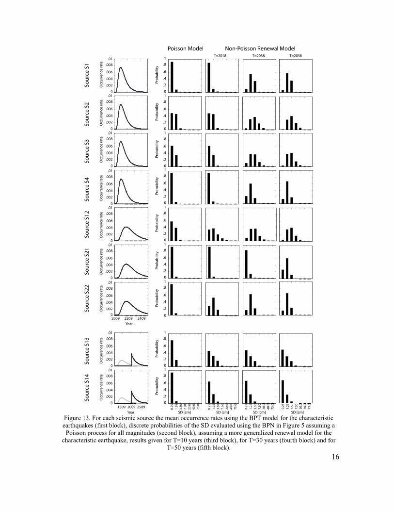
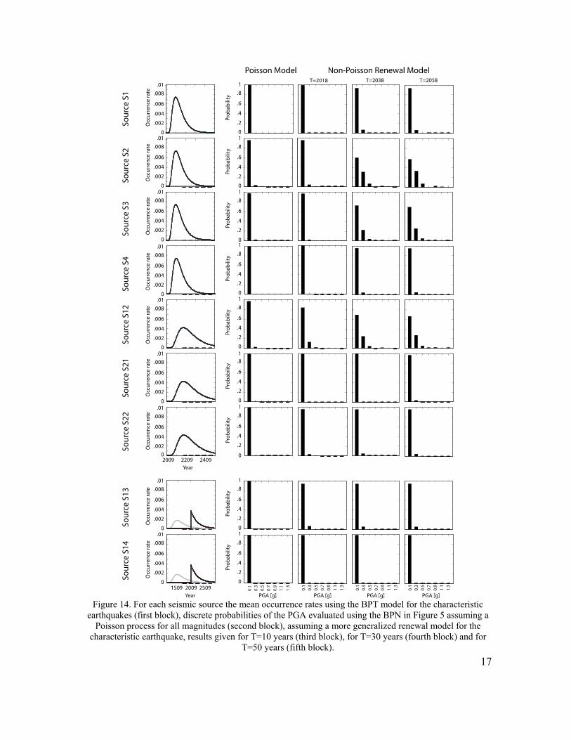
is the fundamental period of the structures considered in the accompanying paper (Bayraktarli and Faber 2009) where the result of these analyses are used. SD is a conditional normal distribution with a mean of PGA and a standard deviation of 21 and discretized also into 10 states. Evaluating each state in PGA from -3.5 to 3.5 with the corresponding correlation coefficient results in conditional probability distributions for SD that are more likely to take extremely large or small values than is PGA (because of the non-zero mean of the conditional distributions).The range of values for the equally spaced 10 discrete states for the node SD is hence taken from -5 to 5. For each of the nine segments in the zonation model and each of the 50 years a BPN as given in Figure 5 is constructed. The probability tables of the five nodes other than the magnitude node are constructed with the specification of the segments. For the magnitude node the probability tables are calculated for each year according to the Equations 13-14 (see Figure 9). Thus 450 BPN’s are constructed, which yield a marginal distribution for PGA and SD for each segment and each year through evaluation of the corresponding BPN. In Figure 13 and Figure 14 sample results for each segment for the years 2018, 2038 and 2058 are given. The distributions of PGA and SD for each segment are also given for the case, when the occurrence of all the magnitudes is modelled as Poisson events. As the distribution of PGA and SD are calculated with the condition that at least one earthquake larger than Mw=5 will occur, the final results when using the output for further analyses have to be multiplied by the rate of exceeding Mw=5.

16

Figure 13. For each seismic source the mean occurrence rates using the BPT model for the characteristic earthquakes (first block), discrete probabilities of the SD evaluated using the BPN in Figure 5 assuming a

Poisson process for all magnitudes (second block), assuming a more generalized renewal model for the characteristic earthquake, results given for T=10 years (third block), for T=30 years (fourth block) and for

T=50 years (fifth block).

17

Figure 14. For each seismic source the mean occurrence rates using the BPT model for the characteristic

earthquakes (first block), discrete probabilities of the PGA evaluated using the BPN in Figure 5 assuming a Poisson process for all magnitudes (second block), assuming a more generalized renewal model for the

characteristic earthquake, results given for T=10 years (third block), for T=30 years (fourth block) and for T=50 years (fifth block).

18

8. Conclusions An alternative calculation and representation scheme for the standard Probabilistic Seismic Hazard Analysis (PSHA) using Bayesian Probabilistic Networks (BPN) is presented. BPN’s allow for easy calculation of the marginal probability distribution of any parameter within the model as well as the calculation of the joint probability distribution for a subset or all of the parameters. The BPN is easily extended to compute joint probability distributions for multiple ground motion parameters—a feature not easily implemented in standard PSHA. Backward calculation, as implemented using deaggregation in standard PSHA, can also easily be performed using BPN’s. One critical issue in constructing BPN’s is the discretisation of the parameters within the model. The sensitivity of the results on the discretisation scheme is discussed in the accompanying paper of Bayraktarli and Faber (2008), as here the general application of the methodology and the input for the risk study is calculated. Incorporation of model choice uncertainties and time-dependant seismic hazard into the BPN model for seismic hazard are also discussed. Finally, the uncertainty treatment in earthquake modeling using BPN is illustrated on the region Adapazari, which is located close to the western part of the North Anatolian Fault in Turkey. Discrete probabilities for spectral displacement and peak ground acceleration are calculated for Adapazari using BPN’s. These results will be used in the accompanying paper in this special edition, where several aspects regarding seismic risk are discussed (Bayraktarli and Faber 2008). Acknowledgements The support provided by the Swiss National Science Foundation for the research project “Management of Earthquake Risks using Condition Indicators” (MERCI, 2008) is greatly acknowledged. References Abrahamson N. A and Silva W. J., Empirical Response Spectral Attenuation Relations for Shallow

Crustal Earthquakes. Seismological Research Letters, 1997, Vol. 68, pp. 94-126. Abrahamson N., Birkhaeuser P., Koller M., Mayer-Rosa D., Smit P., Sprecher C., et al. Pegasos—

A comprehensive probabilistic seismic hazard assessment for nuclear power plants in Switzerland. Proc. 12th European Conf. on Earthquake Eng., London, 2002, Paper no: 633.

Anagnos, T. and Kiremidjian, A. S., A review of earthquake occurrence models for seismic hazard analysis. Probabilistic Engineering Mechanics, 1988, Vol. 3, Issue 1, 3-11.

Atakan, K., Ojeda, A., Meghraoui, M., Barka, A. A., Erdik, M., Bodare, A., Seismic hazard in Istanbul following the 17 August 1999 Izmit and 12 November 1999 Düzce earthquakes. Bulletin of the Seismological Society of America, 2002, Vol. 92, Issue 1, pp. 466-482.

Baker, J. W., Correlation of ground motion intensity parameters used for predicting structural and geotechnical response. Proceedings 10th International Conference on Applications of Statistics and Probability in Civil Engineering, Tokyo, 2007.

Baker J. W. and Cornell C. A., Correlation of Response Spectral Values for Multi-Component Ground Motions. Bulletin of the Seismological Society of America, 2006, Vol. 96, pp.215-227.

Bayraktarli, Y. Y., Faber, M. H., Bayesian probabilistic network approach for managing earthquake risks of cities, submitted to Georisk, 2009.

Bazzurro P. and Cornell C. A., Seismic Hazard Analysis of Nonlinear Structures I: Methodology. Journal of Structural Engineering, 1994, Vol. 120, pp.3320-3344.

19

Boore, D. M., Joyner, W. B., Fumal, T. E., Equations for Estimating Horizontal Response Spectra and Peak Acceleration from Western North American Earthq.: A Summary of Recent Work. Seismological Research Letters, 1997, Vol. 68/1.

Cetin, K. O., et al., Standard Penetration Test-Based Probabilistic and Deterministic Assessment of Seismic Soil Liquefaction Potential. Journal of Geotechnical and Geoenvironmental Engineering, 2004, Vol. 130, pp. 1314-1340.

Coppersmith, K. J. and Youngs, R. R., Capturing uncertainty in probabilistic seismic hazard assessments with intraplate tectonic environments. Proceedings, 3rd U.S. National Conference on Earthquake Engineering, Charleston, South Carolina, 1986, Vol. 1, pp.301-312.

Cornell, C. A., Engineering seismic risk analysis. Bulletin of the Seismological Society of America, 1968, Vol. 58, pp. 1583-1606.

Cornell C. A, et al., Probabilistic Basis for 2000 SAC Federal Emergency Management Agency Steel Moment Frame Guidelines. Journal of Structural Eng., 2002, Vol. 128, pp. 526-533.

DRM, World Inst. for Disaster Risk Management Inc. and General Directorate of Disaster Affairs, Seismic Microzonation for Municipalities, 2004, www.DRMonline.net

Erdik, M., Demircioglu, M., Sesetyan, K., Durukal, E., Siyahi, B., Earthquake hazard in Marmara Region, Turkey. Soil Dynamics and Earthquake Engineering, 2004, Vol. 24, pp. 605-631.

Gutenberg, B. and Richter, C. F., Frequency of earthquakes in California, Bulletin of the Seismological Society of America, 1944, Vol. 34, pp. 185-188.

Hugin, Version 6.8, 2008, Software, www.hugin.com Jensen, F. V., Bayesian Networks and Decision Graphs, 2001 (UCL Press Limited). Kramer, S. L., Geotechnical Earthquake Engineering, 1996 (Prentice-Hall). Kramer S. L., Mayfield R. T., Anderson D. G., Performance-Based Liquefaction Evaluation:

Implications for Codes and Standards. Proceedings 8th US National Conference on Earthquake Engineering, San Francisco, 2006.

Kulkarni, R. B., Youngs, R. R., Coppersmith, K. J., Assessment of Confidence Intervals for Results of Seismic Hazard Analysis. Proceedings of the Eighth World Conference on Earthquake Engineering, San Francisco, 1984.

Matthews, M. V., Ellsworth, W. L., Raesenberg, P. A., A Brownian model for recurrent earthquakes. Bulletin of the Seismological Society of America, 2002, Vol. 92, pp. 2233-2250.

McGuire, R., Probabilistic Seismic Hazard Analysis and Design Earthquakes: Closing the Loop, Bulletin of the Seismological Society of America, 1995, Vol. 85, Issue 5, pp. 1275-1284.

NRC, Panel on seismic hazard evaluation, Review of recommendations for probabilistic seismic hazard analysis: guidance on uncertainty and use of experts, National Research Council, 1997.

Pinto P. E., Giannini R., Franchin P., Seismic Reliability Analysis of Structures, 2004 (IUSS Press Pavia).

Reid, H. F., The elastic rebound theory of earthquakes. Bulletin of the Department of Geology, University of California, Berkeley, CA, 1911, Vol. 6, pp. 413-444.

SSHAC 1997, Senior Seismic Hazard Analysis Committee 1997: Recommendations for probabilistic seismic hazard analysis: Guidance on uncertainty and use of experts. U.S. Nuclear Regulatory Commission, 1997, NUREG/CR-6372.

Stepp J. C., Wong I., Whitney J., Quittmeyer R., Abrahamson N., Toro G., et al, Yucca Mountain PSHA project members. Probabilistic seismic hazard analyses for ground motions and fault displacements at Yucca mountain, Nevada. Earthquake Spectra, 2001, Vol. 17, pp. 113–51.

Takahashi, Y., Der Kiureghian, A., Ang, A. H.-S., Life-Cycle cost analysis based on a renewal model of earthquake occurrences. Earthquake Engineering & Structural Dynamics, 2004, Vol. 33, pp. 859-880.

Youd, T. L. et al. Liquefaction Resistance of Soils: Summary Report from the 1996 NCEER and 1998 NCEER/NSF Workshops on Evaluation of Liquefaction Resistance of Soils. Journal of Geotechnical and Geoenvironmental Engineering, 2001, Vol. 127, pp. 817-833.