mobile lidar-based convergence detection in underground
TRANSCRIPT

Mobile LiDAR-based convergence detection in underground tunnel
environments
Brian K. Lyncha,∗, Jordan Marrb, Joshua A. Marshalla,b, Michael Greenspanb
aThe Robert M. Buchan Department of Mining, Queen’s University at Kingston bDepartment of Electrical and Computer Engineering, Queen’s University at Kingston
Abstract
This paper presents a mobile LiDAR-based method for remotely identifying convergence (i.e., naturally occurring
deformation) in excavated underground tunnel environments. A mobile LiDAR system is used to collect and
generate two independent 3D point clouds of the excavated environment. In the absence of actual convergence,
simulated deformation is applied to one of the two point clouds based on a simple convergence model.
Registration of the 3D data is performed by using a rough alignment based on principal components, followed
by a piecewise iterative closest point (ICP) algorithm. The residual point-to-surface distances are then used as a
deformation signal, which is filtered using a modal analysis based on expected deformation shapes as well as a
median filter. It was found that convergence deformations of 0.05 m could be confidently identified and
deformations as low as 0.0125 m could be detected within residual deformation data with a mean absolute error
of approximately 0.0235 m. The proposed technique therefore allows deformations on the same order as
background noise to be characterized and flagged for further inspection by mine operators.
Keywords: convergence, LiDAR, frequency analysis, signal processing
1. Introduction
Underground tunnels, shafts, and drifts are subject
to enormous stresses caused by the loads distributed
in the surrounding rock. The stress field around these
excavated openings leads to inelastic deformation
that causes them to slowly close—a phenomenon
known as convergence. Measuring and understanding
convergence is important to geoscientists and
engineers who operate in underground tunnel
environments. Convergence in underground mining is
a particularly serious concern, causing damage to
equipment and infrastructure, project delays and
production losses, as well as posing a significant risk
to human safety.
Typical convergence monitoring involves the use of
instrumentation installed at strategic locations for
directly measuring displacement or strain.
Instruments called telltales are often installed inside
drilled holes, with one end anchored and the other
end protruding outwards with a colour-coded
indicator [1]. These mechanical devices show the
amount of movement of the anchored point with
respect to the rock face. Electronic telltales can be
used to provide a linked network
∗ Corresponding author. Email addresses: [email protected] (Brian K.
Lynch), [email protected] (Jordan Marr),
[email protected] (Joshua A. Marshall),
[email protected] (Michael Greenspan) URL: msl.engineering.queensu.ca (Joshua A. Marshall)
that continuously monitors deformation throughout
the mine. Various types of extensometers are also
available for monitoring deformation between the
floor and back or between walls. Using a tape or
telescopic rod and a position sensor such as a linear
variable displacement transducer, extensometers can
provide precise measurements on location or
remotely [2, 3]. Monitoring systems based on
computer vision have also been developed and
tested. These typically use a digital camera to track
the movement of a reflective target plate [4, 5].
Another method for measuring deformation in
underground environments is the use of
photogrammetry, where a 3D model is generated
from 2D photographic data and used to estimate
volume changes [6].
1.1. Background
The current state-of-the-art in underground
surveying and mapping is the use of stationary laser

2
range measurement systems based on light detection
and ranging technology (LiDAR), which has become an
invaluable tool for many applications in mining and
geotechnics [7, 8, 9, 10]. Previous work has
demonstrated the feasibility of detecting changes
based on
comparisons of LiDAR scans captured before and after
deformation has occurred. The simplest method for
detecting deformation is to compute the distance
between nearest corresponding points in each scan
(Hausdorff distance) [11, 12, 13]. Another approach is
the use of minimum-distance projection to compare
subsequent scan data and determine local
deformations [14]. An improvement on the point-to-
point method is to generate meshed surfaces from
scan data and compute surface-to-surface distances
to detect changes [15, 16]. Deformations in circular
tunnel cross-sections have been analyzed by fitting
ellipses to scan data and comparing the change in
shape [17]. Deformation in tunnels has also been
investigated by comparing LiDAR scan data to
previously surveyed models [18, 19]. In many cases,
alignment and registration of scan data depends on
the use of designated control points that are often
carefully surveyed within a known coordinate system
[20, 21]. It is important to note that stationary LiDAR
scanning is typically laborious and time-consuming,
and often requires that operations be ceased in the
vicinity of the survey.
1.2. About this Paper
This paper presents a method for remote
convergence detection that uses relatively low-cost
LiDAR devices mounted on a mobile platform (e.g., a
vehicle), which is used to repeatedly scan areas of
interest. The approach presented in this paper builds
on recent advances in the field of simultaneous
localization and mapping (SLAM), where LiDAR and
inertial measurement unit (IMU) data are fused in
order to estimate sensor motion and create 3D point
clouds of underground environments where a global
positioning system (GPS) is unavailable. Compared
with the use of stationary LiDAR surveys, this method
is prone to larger errors and higher uncertainty, but
can provide acceptable results in significantly less
time. In this research, two LiDAR scans of the same
underground mine environment were generated
from a mobile platform and used to study a method
for convergence detection. Although actual
convergence deformation from two time-separated
scans would be preferable, simulated deformation
was added to one scan due to constraints on data
collection and the unavailability of reference
measurements. The use of simulated deformation
also provided ground-truth for evaluating the
accuracy of the convergence detection algorithm.
The results presented in this paper were derived
from data collected using the uGPS Rapid MapperTM
(RM) system—see Fig. 1—although any similar system
could have been used. It consists of two orthogonally-
mounted 2D LiDAR devices and an IMU. The device is
vehicle-mounted and collects data that is
subsequently processed to form a 3D map of the
environment. Surveyed markers are also used
intermittently to affix the map within a global
coordinate frame and reduce uncertainty [22]. Fig. 2
shows an example of two point clouds covering the
same region in an underground mine, generated using
the RM system.
Point cloud data generated from a mobile LiDAR
platform has been successfully used to generate as-
Figure 1: The uGPS Rapid MapperTM (RM) mobile LiDAR scanning system, mounted to the trailer hitch of a vehicle [photo: Peck Tech Consulting].
Figure 2: Example of two RM point clouds covering the same region. One point cloud is shown in blue, with the other shown in grey for comparison.
built models of tunnel environments [23].
Furthermore, change detection in mobile LiDAR data
has also been studied previously, demonstrating
detection of changes in features as small as 20 cm
[24]. The primary challenge when analyzing mobile
LiDAR data to detect convergence is the high level of
uncertainty associated with the reconstructed point
cloud data (typically on the same or greater order of
Preprint submitted to Computers and Geotechnics April 6, 2017
3
magnitude as the expected convergence
deformation). This low signalto-noise ratio makes
direct comparison of two subsequent data sets
impractical. In addition, drift due to imperfect inertial
navigation causes dead reckoning errors which can
vary significantly between subsequent surveys.
Mobile LiDAR data is also much more sparse
compared to stationary LiDAR data, resulting in less
detail. Therefore, more sophisticated signal
processing techniques are required to confidently
detect convergence in mobile LiDAR scans. Although
error and uncertainty in stationary LiDAR data has
been studied [25] and may be included as part of an
analysis of mobile LiDAR data, the specific variances
of the reconstructed RM data were unavailable for
this study.
Before analyzing the data to characterize
deformation, the two data sets must be registered to
minimize errors due to sensor drift. This process is
achieved by using a piecewise version of the point-to-
plane iterative closest point (ICP) algorithm [26]. The
out-of-plane distances that remain when comparing
the registered data sets are then assumed to be the
measured deformation along with a large amount of
noise. The measured deformation is then analyzed to
determine lowfrequency responses represented by
expected convergence deformation modes, and the
resulting responses smoothed with a median filter to
further reduce noise. The experiments reported by
this paper found that deformations of 50 mm were
confidently identified by using a LiDAR-based mobile
mapping system such as the RM system employed
here, but that deformations as low as 12.5 mm may
be detectable.
2. Data, Modelling, and Simulation
Convergence is complex and non-uniform due to
the stress field in the surrounding rock structure, and
displacement of a tunnel face occurs generally in any
direction. However, a simplified model was adopted
for this study, where displacement was assumed to
occur only in the out-of-plane direction (i.e.,
displacement along the tunnel or around its
perimeter was ignored).
2.1. Data Structure
The RM system generates a point cloud by
estimating the sensor pose using a combination of
horizontal scan matching and inertial navigation, and
transforming laser range measurements into an
inertial reference frame (see [22] for further details).
Data from an additional vertically-installed scanner is
used to generate a 3D point cloud. The employed SICK
LMS 111 laser scanner measures range at 541 points
as it sweeps across an angular window of 270◦, with
position and orientation of the sensor estimated at a
rate of 10 Hz, for a total of 5410 points per second.
A dataset is therefore composed of a series of scan
slices with points defined in a Cartesian inertial
reference frame. The data may also be represented in
a quasi-cylindrical coordinate system where the laser
range and angle form the polar coordinates, but the
linear axis is replaced with an axis that follows the
sensor path (defined by scan slice index, j). Out-of-
plane displacement is provided as a result of the
piecewise ICP registration process, but convergence
deformation is reduced to displacement in the radial
direction with respect to the tunnel centroid at each
scan slice.
2.2. Convergence Model
The amplitude of deformation at each point in a
dataset is defined by a scalar displacement map, δ.
Each point is then displaced in the corresponding
radial direction by the appropriately indexed value of
the displacement map.
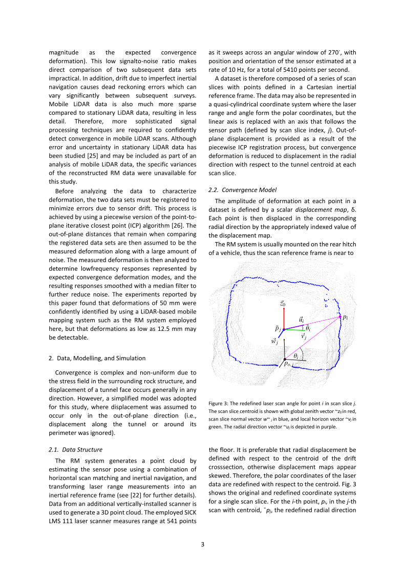
The RM system is usually mounted on the rear hitch
of a vehicle, thus the scan reference frame is near to
Figure 3: The redefined laser scan angle for point i in scan slice j.
The scan slice centroid is shown with global zenith vector ~z0 in red,
scan slice normal vector w~ j in blue, and local horizon vector ~vj in
green. The radial direction vector ~uj is depicted in purple.
the floor. It is preferable that radial displacement be
defined with respect to the centroid of the drift
crosssection, otherwise displacement maps appear
skewed. Therefore, the polar coordinates of the laser
data are redefined with respect to the centroid. Fig. 3
shows the original and redefined coordinate systems
for a single scan slice. For the i-th point, pi, in the j-th
scan with centroid, ¯pj, the redefined radial direction

4
is given by ~ui. The scan angle is also redefined as θ˜i
based on the radial direction vector and local horizon.
Modal shape functions are then used to model
convergence deformation. These mode shapes are
defined as a function of the laser scan angle with
respect to the scan slice centroid. Two deformation
modes were used for this study: 1) a uniform mode,
and 2) a squeezing mode. Modes are then combined
to form more complex overall deformation
distributions. This approach for modelling
deformation in underground tunnels has previously
been used for analytical and numerical studies [27].
Fig. 4 shows the deformation modes applied to a
circular drift cross-section and a sample crosssection
from an RM dataset.
The uniform mode applies constant deformation,
resulting in a modal function, η1, that is simply unity
across the entire scan slice
η1 = 1. (1)
The squeezing mode applies inward deformation to
the floor and back and outward deformation to the
walls. This was achieved by using a cosine modal
function
η2 = cos2θ.˜ (2)
Equation 3 defines the total modal displacement
for a single scan slice where ψj,k is the amplitude of the
Figure 4: Top: Deformation mode shapes applied to a circular tunnel cross-section (original data in black and deformed data in blue). Bottom: Deformation mode shapes applied to a sample tunnel crosssection from a RM dataset (original data in black and deformed data in blue).
k-th mode over the j-th scan slice,
M X
δj = ψj,kηk. (3) k=1
The total deformation across a scan slice due to the
linearly combined modes with respective modal
deformation magnitudes ψj,1 and ψj,2 is given by
δj = ψj,1η1 + ψj,2η2. (4)
The total deformation may also be defined as the
matrix product of the modal matrix, H, and modal
amplitude vector, ψ~ j, as shown in
H = hη1 η2i
(5) " #
ψ~ j = ψj,1 (6) ψj,2
δj = Hψ~ j (7)
The modal matrix, H, is the concatenation of the mode
shape column vectors evaluated at the laser scan
angles θ˜. Given the displacement δj across a scan
slice, the mode amplitudes ψ~ j may be determined by
inverting Equation 7 using the Moore-Penrose
pseudoinverse
ψ~ j = HT H−1 HTδj. (8)
The modal deformation functions apply only to the
2D drift cross-section, therefore varying the
magnitudes across scan slices is necessary to achieve
3D effects. For simulation, the cross-section
deformation is specified as a function of scan slice
index, j, using continuous sigmoid functions to define
a region of constant deformation amplitude.
Convergence deformation is simulated on a RM
dataset across four separate regions. The uniform and
Squeezing Mode Uniform Mode
UNIFORM SQUEEZING

5
Figure 5: Simulated convergence deformation applied to a RM dataset with radial displacement specified in metres, positive inwards. Top: applied modal amplitudes across scan slices. Bottom: radial displacement visualized over RM dataset.
squeezing modes are each applied individually over
the first two regions, both modes are applied in
combination over the third region, and non-modal
deformation is applied over the fourth region by
displacing the tunnel outwards in the lateral direction
only. Figure 5 shows the applied modal amplitudes as
a function of scan index number as well as the radial
displacement visualized over the RM dataset. Note
that smooth, continuous sigmoidal functions are used
but the applied modal amplitudes vary slightly across
scan indices due to the variation in scan angle with
respect to the scan slice centroid.
3. Registration
Datasets generated using the RM system suffer
from local errors—typically ±3 cm, based on
experiments 1 —too large to allow for direct
comparison as a method for detecting convergence.
In addition, repeated scans from exactly the same
sensor pose is impractical. Therefore, registration of
the datasets using a piecewise transformation
technique is necessary to enable a proper
comparison.
The registration process is composed of three
phases: 1) preparation; 2) rough alignment; and, 3)
1 As reported at www.ugpsrapdimapper.com (March 7, 2016).
piecewise transformation. The preparation phase
involves manual selection and trimming of two
datasets covering a common region of interest. Rough
alignment then matches the centroids and principal
axes of both data sets by transforming the query
dataset. The fixed and roughly-aligned query datasets
are then passed to an algorithm that registers sections
of the query dataset within the fixed data set.
The registration method used in this paper is based
on the iterative closest point (ICP) algorithm, which
rigidly transforms a query point cloud to match a
reference point cloud. ICP typically attempts to
minimize point-to-point or point-to-surface distances
between matched points in the two clouds, and many
variants of the ICP algorithm have been studied.
Others have implemented non-rigid registration by
using generalized methods for matching a deformed
query point cloud to a reference model that accounts
for significant noise, occlusions, and outlying points
[28]. However, this paper is concerned with finding an
appropriate non-rigid registration to remove drift in
the reconstructed query point cloud while still
retaining small deformations due to actual
convergence. A similar problem that involves non-
rigid registration of laser range data from an
unmanned helicopter was investigated in [29], where
drift in the motion model was compensated within
the registration process.
Point cloud data from the RM system is
reconstructed independently for each individual data
set, therefore non-rigid registration cannot be applied
based on the motion model. Instead, it is assumed
that drift is negligible for small subsections of data,
allowing rigid point-to-plane ICP registration to be
performed for each individual scan slice based on a
window of surrounding data and resulting in a
piecewise rigid registration method. The
transformation for each subsection is then applied
only to the centre scan slice during reconstruction.
In this paper, the preparation and rough alignment
phases were computed using MATLAB R scripts. The
piecewise transformation was computed using C++
scripts based on Point Cloud Library (PCL) functions.
3.1. Preparation
Two datasets are selected that cover an
overlapping region of an underground tunnel and
extracted by using the RM software. The datasets are
then examined and manually trimmed to cover only
the overlapping region of interest. For example,
consider the two datasets shown in Figure 6, each

6
covering the same general area of an underground
mine.
3.2. Rough Alignment
The centroid of each data set is computed by
finding the average position of the point cloud data.
Before computing the centroid, the point cloud is
filtered
Figure 6: Example of a pair of trimmed Rapid Mapper point clouds before rough alignment.
Figure 7: Example of the trimmed point clouds after rough alignment.
to ensure that the point density is relatively uniform
and to avoid biasing the centroid position. This is
accomplished by truncating the point cloud position
data based on a selected resolution and keeping only
unique points, resulting in an occupancy grid data
format. The same filtered point cloud is then used to
determine the moment of area tensor from which the
principal components of each data set are extracted.
The principal axes represent the orientation of the
data set reference frame within the global coordinate
system. The original query data set point cloud is then
transformed into the fixed data set reference frame
based on the position offset and rotation. Figure 7
shows trimmed point clouds after rough alignment,
resulting in an imperfect but acceptable initial
registration of the two data sets.
3.3. Piecewise Registration
To obtain the results in this paper, the fixed and
query data point clouds were exported from MATLAB
R to point cloud data (PCD) format. These files were
passed to a C++ script that computed surface normals
using PCL functions (based on a PCA algorithm) and
performed the piecewise ICP registration for
successive sections of the query data set, storing the
transformations and outputting to a delimited ASCII
text file.
The registration algorithm iterates through each
scan slice of the query data set, sampling a window of
data centred on the current query slice and
registering that window of the query point cloud with
a window of the
Figure 8: Example of the trimmed point clouds after non-rigid ICP alignment.
fixed point cloud. The fixed point cloud window is
selected based on a mapping of the nearest centroids
for the bounding indices of the query data window,
reducing the number of points being considered and
speeding up the overall process. Margins are also
added to the bounding indices to account for error
remaining after rough alignment.
The point-to-plane ICP algorithm is then applied to
the fixed and query point cloud windows. The query
point cloud window is transformed to minimize the
sum of the squared out-of-plane distances between
each point in the query data and the nearest point in
the fixed data (i.e., projected along the normal
direction of the fixed data point). After the ICP
algorithm has converged, the resulting translation
and rotation transformation is stored and the
algorithm continues to the next scan slice index.
Although the registration process is performed
using a rigid transformation for windowed sections of
the data, the solved transformation is applied only to
the centre scan slice. Therefore, each scan slice is
transformed independently but based on registration
of a surrounding window of data, resulting in a
nonrigid transformation of the overall point cloud. For
the results in this paper, a C++ script outputs a
delimited ASCII text file containing the translation and
rotation data for each scan slice. Final reconstruction
of the query point cloud was performed by using a
MATLAB R script.

7
Figure 8 shows the results of piecewise registration
of the previously rough aligned query data set.
Comparison of Figure 7 and Figure 8 demonstrates
noticeable improvement in the alignment of the two
datasets. Table 1 presents the mean, median, and
standard deviation of the absolute out-of-plane
distances after rough alignment and after non-rigid
ICP alignment. Note that the registration results are
presented for the case with no convergence
deformation added, therefore the residual out-of-
plane distances are strictly the result of errors due to
sensor uncertainty, point cloud reconstruction, and
registration. Table 1: Point-to-plane distance statistics after rough alignment and piecewise non-rigid registration.
Parameter Rough Piece-wise
Mean (m) 0.6398 0.0211
Median (m) 0.3461 0.0144
Std. Dev. (m) 0.7723 0.0235
4. Post Processing & Analysis
The residual point-to-plane distances after
piecewise registration represent the deformation of
the tunnel and are output as a measured
displacement map to be post-processed. However,
significant noise corrupts the displacement map due
to the presence of measurement uncertainty during
data collection, registration errors during generation
of the RM data set, and registration errors during the
rough alignment and piecewise registration
processes. The amplitude of the noise in the
displacement signal is within the same order of
magnitude as the amplitude of expected convergence
deformation. Therefore, inspection of the raw
displacement map is not sufficient for identifying
regions undergoing convergence, and post-processing
is necessary to suppress noise and highlight
convergence deformation.
Noise in the displacement map is randomly
distributed across each point and characterized by
high spatial frequencies, whereas convergence
deformation is modelled using mode shapes that are
characterized by low spatial frequencies. The mode
amplitudes for each scan slice were determined from
the displacement map by applying the inverse
transformation given by Equation 8. These mode
amplitudes were then further reduced to a single
value at each scan slice by evaluating the norm of the
mode amplitude vector
q
ψ¯ = ψ~Tψ.~ (9)
Mode analysis is applied to each scan slice
individually (i.e., around the circumference of the
tunnel) but does not suppress noise along the tunnel.
A median filter with a window of 81 scan slices is
therefore applied along the tunnel to further reduce
noise in the mode amplitude norm signal.
Although mine operators may be interested in
inspecting the individual mode responses or even the
raw displacement map, the filtered mode amplitude
norm, ψ¯, provides a single scalar value at each scan
slice that indicates the estimated amount of
convergence deformation present.
The overall process of rough alignment, piecewise
non-rigid registration, and post-processing is
summarized in the flow chart shown in Figure 9.
Figure 9: Flow chart describing the overall algorithm.
5. Results & Discussion
Registration and post-processing were performed
for the pair of real RM datasets shown in Figure 2 with
simulated convergence deformation of various
amplitudes applied to the query dataset prior to
registration. Real data with actual convergence
deformation was not available, therefore simulated
convergence deformation was necessary and also
provided a known groundtruth for comparison. Based
on discussions with practitioners, the desired
minimum observable deformation magnitude was
0.05 m. This is the amount of deformation that should
Fixed Scan Query Scan
Rough Alignment
Non - Rigid Registration
Out - of - plane error analysis
Modal Response
Median Filter
Rough - aligned query scan
Registered query scan
Displacement map
Norm of mode amplitudes
Convergence deformation

8
evoke action such as detailed inspection or structural
reinforcement. The analyses were also performed
without any deformation applied in order to provide
a baseline comparison. Although this would not be
possible with real convergence deformation, it allows
the combined error due to sensor uncertainty,
original data reconstruction, and registration to be
evaluated independently of applied deformation.
Analyses were performed using the simulated
convergence deformation model shown in Figure 5
with mode amplitudes corresponding to convergence
deformation of 0.05 m, 0.0375 m, 0.025 m, and
0.0125 m. The deformed query dataset was then
registered to the fixed dataset and the resulting
displacement map was analyzed to determine the
medial-filtered norm of the mode amplitudes.
Figure 10 shows the absolute value of the
displacement maps for the applied deformation, the
results after registration with no applied
deformation, and the results after registration with
0.05 m applied deformation. It can be seen that
there are regions with relatively high residual error
even with no applied deformation (most notably
around scan slice 1100). These regions of high
residual error represent false positives that may be
interpreted as convergence deformation when in
fact they are the result of error accumulated during
the original data reconstruction and piecewise
registration processes. The results after registration
of the data with 0.05 m applied deformation show
identifiable regions of convergence but there exists
relatively large amounts of noise in the surrounding
regions without any actual applied deformation.
Inverse modal analysis of the displacement map
based on the use of Equation 8 yields the results
shown in Figure 11. The mode amplitude response for
both uniform and squeezing modes is still corrupted
by a significant amount of noise, but shows a better
correspondence with the applied mode amplitudes.
Figure 11 shows the results after taking the norm of
the mode amplitudes as well as with the application
of the median filter. It can be seen that the resulting
response after application of the median filter
successfully suppresses noise and more closely
matches the applied deformation.
Figure 12 shows the norm of mode amplitudes for
results with various magnitudes of applied
deformation after applying the median filter, along
with the norm of mode amplitudes for the actual
applied deformation. The results for the case with no
applied deformation are also included for
comparison. Each response underestimates the
convergence deformation but the overall result is that
regions of convergence are clearly discernible after
computing the norm of the modal response and
applying the median filter.
Using the approach presented in this paper, target
convergence deformations of 0.05 m are apparent to
an operator but deformations as low as 0.0125 m may
also be detected. This is emphasized in Figures 13 and
14 where the median-filtered norm of mode
amplitudes and the unprocessed displacement map
are each mapped onto the meshed surface of the scan
data and compared side-by-side for applied
deformations of 0.05 m and 0.0125 m respectively.
While the majority of background noise is
eliminated using the proposed post-processing
technique, there remain some areas of high residual
point-toplane distance that could be falsely identified
as convergence. The primary source of these false
positives are errors in the registration process,
especially at intersections in tunnels where the LiDAR
sensors are exposed to open spaces causing lower
point density and higher reconstruction errors.
Another major source of error is due to the ICP
registration method, which attempts to minimize the
sum of the square of

9
Figure 10: Top: displacement map corresponding to simulated convergence deformation with 0.05 m amplitude. Middle: displacement map after registration of fixed and query data sets with no applied deformation. Bottom: displacement map after registration of fixed and query data sets with 0.05 m applied deformation. Note that absolute displacement is shown.
Figure 11: Top: response of each mode compared to applied deformation. Bottom: norm of mode amplitudes with and without median filter compared to applied deformation. Note these results are for the case with 0.05 m convergence deformation. Figure 12: Norm of mode amplitudes after application of the median filter for various amplitudes of applied deformation compared to actual applied deformations.
200 400 600 800 1000 1200 1400 1600 1800 2000 2200 −0.06 −0.04 −0.02
0 0.02 0.04 0.06 0.08
Uniform (Response) Squeezing (Response) Uniform (Applied) Squeezing (Applied)
200 400 600 800 1000 1200 1400 1600 1800 2000 2200 0
0.02
0.04
0.06
0.08
0.1
0.12
Scan Slice Index
Mode Amplitude Norm Applied Deformation Mode Amplitude Norm (Median Filter)

10
Figure 13: Comparison of unprocessed displacement map and computed mode amplitude norm response mapped onto meshed scan data (0.05 m convergence deformation). Left: unprocessed displacement map. Right: norm of mode amplitudes with median filter applied.
Figure 14: Comparison of unprocessed displacement map and computed mode amplitude norm response mapped onto meshed scan data (0.0125 m convergence deformation). Left: unprocessed displacement map. Right: norm of mode amplitudes with median filter applied.
the point-to-plane distances based on rigid
transformation of the data window being considered.
Ideal registration of a deformed data set would result
in zero point-to-plane residual distances at non-
deformed areas, whereas the ICP algorithm spreads
the residual error across all points in the windowed
section. Therefore, point-to-plane distances after
registration are expected to be lower than the applied

11
deformation and result in an underestimation of the
mode amplitudes.
6. Conclusion
The techniques described in this paper
demonstrate that relatively small deformations due
to convergence in underground tunnels may be
efficiently identified by comparison of subsequent
LiDAR data sets captured on a mobile platform.
Although the error and uncertainty in the measured
point cloud data is on the same order of magnitude as
the deformation amplitude, postprocessing
techniques were successful in identifying deformation
signals. By modelling convergence deformation using
expected mode shapes and applying a median filter to
the resulting responses, noise was successfully
suppressed and the target deformation amplitude of
0.05 m was apparent. In addition, convergence
deformations as low as 0.0125 m may be detectable
although with higher risk of falsely characterizing
residual errors as convergence.
Acknowledgment
The authors would like to thank Andy Chapman and
Jamie Lavigne at Peck Tech Consulting for facilitating
access to real underground uGPS Rapid MapperTM
data. Thanks also to Steve McKinnon and Lindsay
Vanderbeck for useful discussions about the
convergence phenomenon.
This project was funded in part by the Natural
Sciences and Engineering Research Council of Canada
(NSERC) under project CRDPJ 44SBO4-12 and by
Barrick Gold Corporation and Peck Tech Consulting.
References
[1] D. Bigby, K. MacAndrew, K. Hurt, Innovations in mine roadway stability monitoring using dual height and remote reading electronic telltales, in: Proceedings of the 2010 Underground Coal Operators Conference, 2010, pp. 146–160.
[2] C. D. Martin, N. A. Chandler, R. S. Read, The role of convergence measurements in characterizing a rock mass, Canadian Geotechnical Journal 33 (2) (1996) 363–370. doi:10.1139/t96014.
[3] D. F. Malan, V. A. Kononov, S. J. Coetzer, A. L. Janse van Rensburg, B. S. Spottiswoode, The feasibility of a mine-wide continuous closure monitoring system for gold mines, Tech. rep., CSIR Miningtek (2000).
[4] D. B. Apel, B. R. Gray, R. H. Moss, S. E. Watkins, T. H. Jones, Development and laboratory trials of the light-based high-resolution target movement monitor for monitoring convergence at underground mines, Journal of Geotechnical and Geoenvironmental Engineering 133 (9) (2007) 1167–1171.
[5] M. Kellaway, D. Taylor, G. J. Keyter, The use of geotechnical instrumentation to monitor ground displacements during excavation of the ingula power caverns, for model calibration
and design verification purposes, Tech. rep., The Southern African Institute of Mining and Metallurgy (2012).
[6] D. J. Benton, S. R. Iverson, L. A. Martin, J. C. Johnson, M. J. Raffaldi, Volumetric measurement of rock movement using photogrammetry, International Journal of Mining Science and Technology 26-1 (2016) 123–130.
[7] S. Fekete, M. Diederichs, M. Lato, Geotechnical and operational applications for 3-dimensional laser scanning in drill and blast tunnels, Tunnelling and Underground Space Technology 25 (2010) 614–628.
[8] S. Fekete, M. Diederichs, Integration of three-dimensional laser scanning with discontinuum modelling for stability analysis of tunnels in blocky rock masses, International Journal of Rock Mechanics & Mining Sciences 57 (2013) 11–23.
[9] M. J. Lato, M. S. Diederichs, Mapping shotcrete thickness using LiDAR and photogrammetry data: Correcting for overcalculation due to rockmass convergence, Tunnelling and Underground Space Technology 41 (2014) 234–240.
[10] M. J. Gallant, J. A. Marshall, Automated rapid mapping of joint orientations with mobile LiDAR, International Journal of Rock Mechanics and Mining Sciences 90 (2016) 1–14.
[11] D. Girardeau-Montaut, M. Roux, R. Marc, G. Thibault, Change detection on points cloud data acquired with a ground laser scanner, International Archives of Photogrammetry, Remote Sensing and Spatial Information Sciences 36 (3).
[12] Z. Kang, Z. Lu, The change detection of building models using epochs of terrestrial point clouds, in: Multi-Platform/MultiSensor Remote Sensing and Mapping (M2RSM), 2011 International Workshop on, 2011, pp. 1–6.
[13] J. Kemeny, K. Turner, Ground-based LiDAR, rock slope mapping and assessment, Tech. Rep. FHWA-CFL/TD-08-006, Federal Highway Administration, U.S. Department of Transportation (2008).
[14] J.-Y. Han, J. Guo, Y.-S. Jiang, Monitoring tunnel profile by means of multi-epoch dispersed 3-D lidar point clouds, Tunnelling and Underground Space Technology 33 (2013) 186– 192.
[15] T. Barnhart, B. Crosby, Comparing two methods of surface change detection on an evolving thermokarst using hightemporal-frequency terrestrial laser scanning, Selawik River, Alaska, Remote Sensing 5 (2013) 2813–2837.
[16] B. A. Slaker, E. C. Westman, B. P. Fahrman, M. Luxbacher, Determination of volumetric changes from laser scanning at an underground limestone mine, Mining Engineering 65-11 (2010) 50–54.
[17] G. Walton, D. Delaloye, M. S. Diederichs, Development of an elliptical fitting algorithm to improve change detection capabilities with applications for deformation monitoring in circular tunnels and shafts, Tunnelling and Underground Space Technology 43 (2014) 336–349.
[18] E. Karampinos, J. Hadjigeorgiou, P. Turcotte, F. MercierLangevin, Large-scale deformation in underground hard-rock mines, Journal of The Southern African Institute of Mining and Metallurgy 115 (2015) 645–652.
[19] T. Nuttens, C. Stal, H. De Backer, G. Deruyter, K. Schotte, P. Van Bogaert, A. De Wulf, Laser scanning for precise ovalization measurements: Standard deviations and smoothing levels, Journal of Surveying Engineering 142-4 (2016) 05016001–1–9.
[20] R. Kukutsch, V. Kajzar, P. Konicek, P. Waclawik, J. Ptacek, Possibility of convergence measurement of gates in coal mining using terrestrial 3D laser scanner, Journal of Sustainable Mining 14 (1) (2015) 30–37.
[21] R. Kukutsch, V. Kajzar, P. Waclawik, J. Nemcik, Use of 3D laser scanner technology to monitor coal pillar deformation, in: Proceedings of 2016 Coal Operators’ Conference, 2016, pp. 99–107.
[22] N. Lavigne, J. Marshall, A landmark-bounded method for large-scale underground mine mapping, Journal of Field Robotics 29 (6) (2012) 861–879.

12
[23] M. Arastounia, Automated as-built model generation of subway tunnels from mobile LiDAR data, Sensors 16-9 (2016) 1486–1505.
[24] W. Xiao, B. Vallet, N. Paparoditis, Change detection in 3D point clouds acquired by a mobile mapping system, in: ISPRS Annals of Photogrammetry, Remote Sensing and Spatial Information Sciences, Volume II-5/W2, 2013, pp. 331–336.
[25] A. Cuartero, J. Armesto, P. Rodriguez, P. Arias, Error analysis of terrestrial laser scanning data by means of spherical statistics and 3D graphs, Sensors 10 (2010) 128–145.
[26] P. J. Besl, N. D. McKay, A Method for Registration of 3-D Shapes, IEEE Transactions on Pattern Analysis and Machine Intelligence 14 (2) (1992) 239–256.
[27] F. Pinto, A. J. Whittle, Ground movements due to shallow tunnels in soft ground, Journal of Geotechnical and Geoenvironmental Engineering 140-4 (2013) 1–17.
[28] T. Fabry, D. Smeets, D. Vandermeulen, P. Suetens, 3d nonrigid point cloud based surface registration based on mean shift, in: WSCG 2010: Full Papers Proceedings: 18th International Conference in Central Europe on Computer Graphics, Visualization and Computer Vision in co-operation with EUROGRAPHICS, 2010, pp. 121–128.
[29] R. Kaestner, S. Thrun, M. Montemerlo, M. Whalley, A nonrigid approach to scan alignment and change detection using range sensor data, in: Field and Service Robotics, Vol. 25 of Springer Tracts in Advanced Robotics, Springer Berlin Heidelberg, 2006, pp. 179–194.