mobile intelligent systems 2004
DESCRIPTION
Mobile Intelligent Systems 2004. Course Responsibility: Ola Bengtsson. Course Examination. 5 Exercises – Matlab exercises – Written report (groups of two students - individual reports) 1 Written exam – In the end of the period. Course information. Lectures - PowerPoint PPT PresentationTRANSCRIPT

Mobile Intelligent Systems 2004
Course Responsibility:
Ola Bengtsson

Course Examination
• 5 Exercises – Matlab exercises – Written report (groups of two students - individual reports)
• 1 Written exam – In the end of the period

Course information
• Lectures
• Exercises (w. 15, 17-20) – will be available from the course web page
• Paper discussions (w. 14-15, 17-21) – questions will be available from the course web page => Course literature
• Web page: http://www.hh.se/staff/boola/MobIntSys2004/
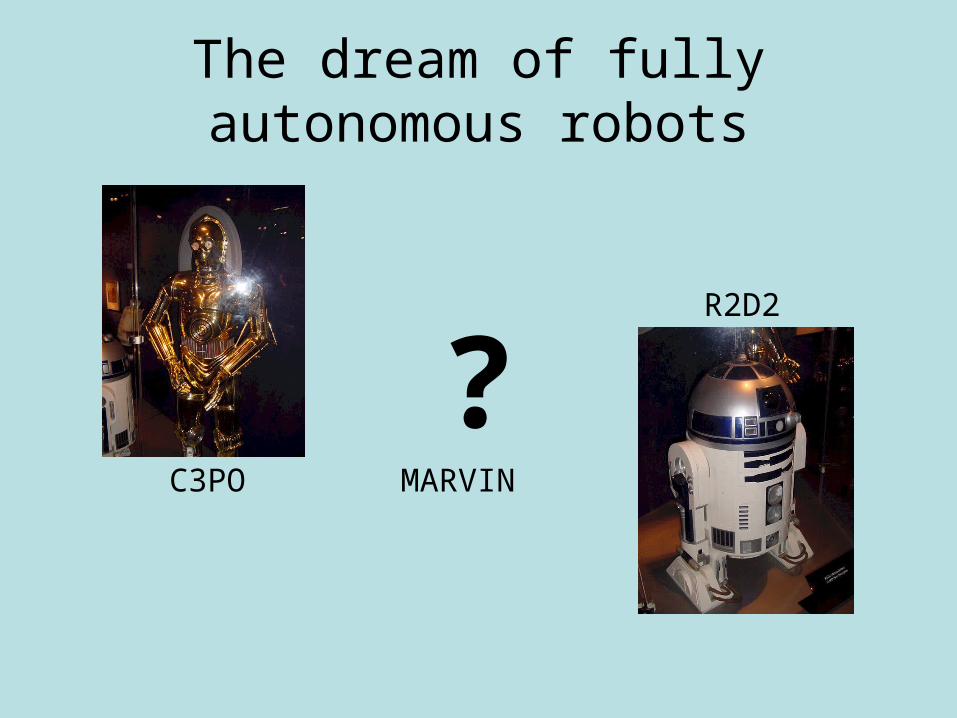
The dream of fully autonomous robots
R2D2
C3PO MARVIN
?

Autonomous robots of today
• Stationary robots- Assembly- Sorting- Packing
• Mobile robots- Service robots
- Guarding- Cleaning- Hazardous env.
- Humanoid robots
Trilobite ZA1, Image from: http://www.electrolux.se
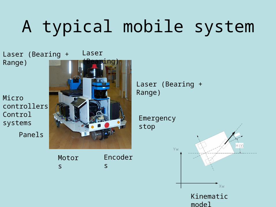
A typical mobile system
H(r)
Xw
Yw
Laser (Bearing + Range)
Laser (Bearing)Laser (Bearing + Range)
EncodersMotors
Panels
Kinematic model
Micro controllers Control systems
Emergency stop

Mobile Int. Systems – Basic questions
• 1. Where am I? (Self localization)• 2. Where am I going? (Navigation)• 3. How do I get there? (Decision making /
path planning)
• 4. How do I interact with the environment? (Obstacle avoidance)
• 5. How do I interact with the user? (Human –Machine interface)

Sensors – How to use them
Micro controller -How to use all these
sensor values
Encoder 1
Gyro 1
Laser
GPS
Gyro 2
Compass
IR
Encoder 2
Ultra sound
Reaction / Decision
Sensor fusion

Course contents
• Basic statistics
• Kinematic models, Error predictions
• Sensors for mobile robots
• Different methods for sensor fusion, Kalman filter, Bayesian methods and others
• Research issues in mobile robotics

Basic statistics – Statistical representation – Stochastic variable
Battery lasting time, X = 5hours ±1hour
X can have many different values
[hours]
P
[hours]
P
Discrete variableContinous variable
Continous – The variable can have any value within the bounds
Discrete – The variable can have specific (discrete) values

[hours]
P
Basic statistics – Statistical representation – Stochastic variable
Another way of discribing the stochastic variable, i.e. by another form of bounds
In 68%: x11 < X < x12
In 95%: x21 < X < x22
In 99%: x31 < X < x32
In 100%: - < X <
The value to expect is the mean value => Expected value
How much X varies from its expected value => Variance
Probability distribution

Expected value and Variance
0 5 10 15 20 250
1
2
3
4
5
6
7
8Lasting time for 25 battery of the same type
dxxfxXE X )(.
k
X kpkXE )(.
dxxfXExXV XX )(.)( 22
K
XX kpXEkXV )(.)( 22
The standard deviation X is the square root of the variance

Gaussian (Normal) distribution
2
2
2
)(
2.
1)( X
XEx
X
X exp
XXmNX ,~
-10 -5 0 5 10 15 200
0.05
0.1
0.15
0.2
0.25
0.3
0.35
0.4Gaussian distributions with different variances
Stochastic Variable, X
Pro
babi
lity,
p(x
)
N(7,1)N(7,3)N(7,5)N(7,7)
By far the mostly used probability distribution because of its nice statistical and mathematical properties
What does it means if a specification tells that a sensor measures a distance [mm] and has an error that is normally distributed with zero mean and = 100mm?
Normal distribution:
~68.3%
~95%
~99%
etc.
XXXX mm ,
XXXX mm 2,2
XXXX mm 3,3

Estimate of the expected value and the variance from observations
0 1 2 3 4 5 6 7 8 9 100
5
10
15
20
25Histogram of measurements 1 .. 100 of battery lasting time
Lasting time [hours]
No.
of
occu
renc
es [
N]
N
kNX kXm
1
1 )(ˆ
N
kXNX mkX
1
21
12 )ˆ)((̂
-10 -5 0 5 10 15 200
0.05
0.1
0.15
0.2
0.25
0.3
0.35
0.4
Lasting time [hours]
p(x)
Estimated distributionHistogram of observations

Linear combinations (1)
+X1 ~ N(m1, σ1)
X2 ~ N(m2, σ2)
Y ~ N(m1 + m2, sqrt(σ1 +σ2))
bXaEbaXE XVabaXV 2
2121 XEXEXXE 2121 XVXVXXV
This property that Y remains Gaussian if the s.v. are combined linearily is one of the great properties of the Gaussian distribution!

Linear combinations (2)
DDND ,~ˆ
5
1
151
51
51
51
51
N
iiN DDDDDDY
We measure a distance by a device that have normally distributed errors,
Do we win something of making a lot of measurements and use the average value instead?
What will the expected value of Y be?
What will the variance (and standard deviation) of Y be?
If you are using a sensor that gives a large error, how would you best use it?

Linear combinations (3)
Ground Plane
a(1)
a(i)
X [m]
Y [m]
theta(i)
dii dd ˆ
iiˆ
di is the mean value and d ~ N(0, σd)
αi is the mean value and α ~ N(0, σα)
With d and α un-correlated => V[d, α] = 0 (Actually the co-variance, which is defined later)
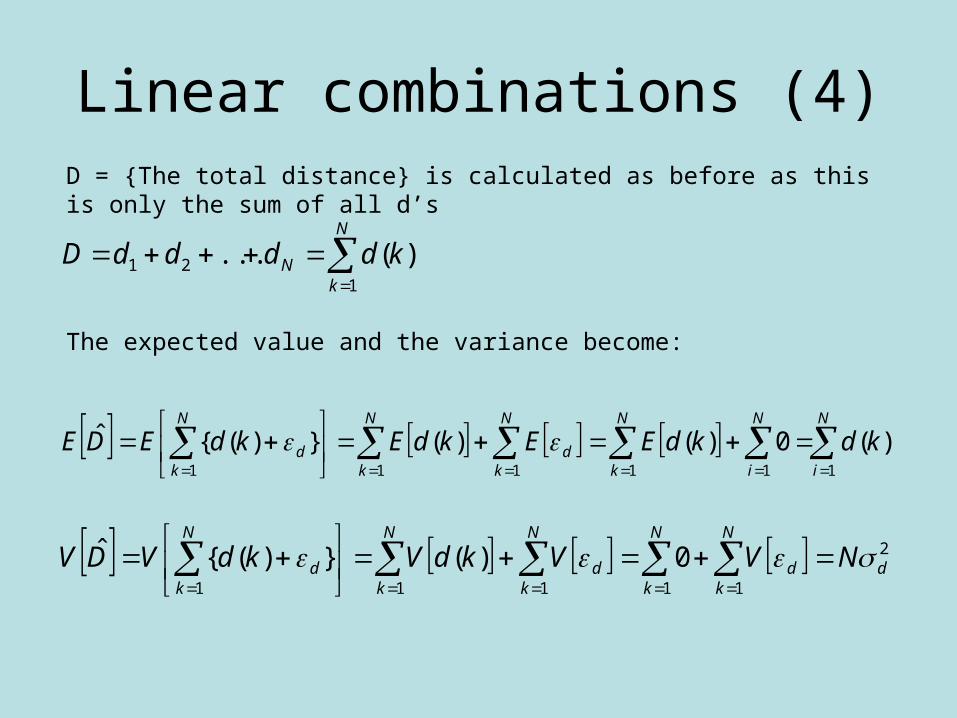
Linear combinations (4)
N
kN kddddD
121 )(...
N
i
N
i
N
k
N
kd
N
k
N
kd kdkdEEkdEkdEDE
111111
)(0)()(})({ˆ
2
11111
0)(})({ˆd
N
kd
N
k
N
kd
N
k
N
kd NVVkdVkdVDV
D = {The total distance} is calculated as before as this is only the sum of all d’s
The expected value and the variance become:
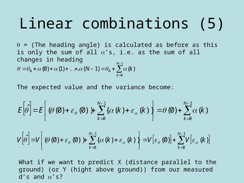
Linear combinations (5) = {The heading angle} is calculated as before as this is only the sum of all ’s, i.e. as the sum of all changes in heading
The expected value and the variance become:
1
000 )()1(...)1()0(
N
k
kN
1
0
1
0
)()0()}()({))0()0((ˆN
k
N
k
kkkEE
1
0
1
0
)()0()}()({))0()0((ˆN
k
N
k
kVVkkVV
What if we want to predict X (distance parallel to the ground) (or Y (hight above ground)) from our measured d’s and ’s?
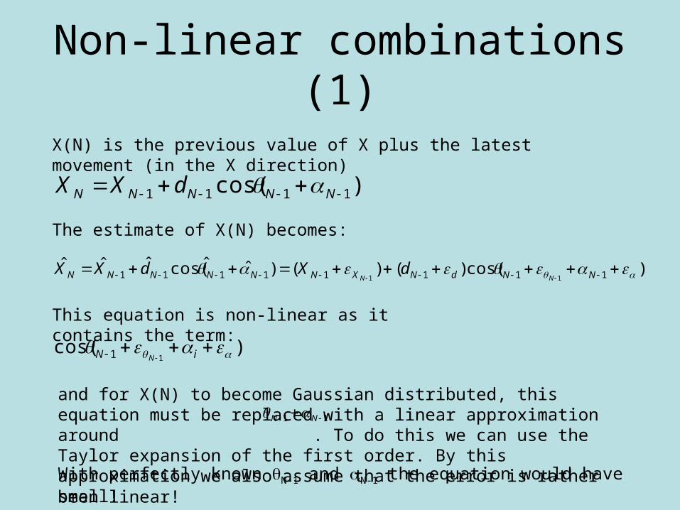
Non-linear combinations (1)
)cos( 1111 NNNNN dXX
X(N) is the previous value of X plus the latest movement (in the X direction)
The estimate of X(N) becomes:
)cos()()()ˆˆcos(ˆˆˆ11111111 11 NNdNXNNNNNN NN
dXdXX
)cos(11 iN N
This equation is non-linear as it contains the term:
and for X(N) to become Gaussian distributed, this equation must be replaced with a linear approximation around . To do this we can use the Taylor expansion of the first order. By this approximation we also assume that the error is rather small!With perfectly known N-1 and N-1 the equation would have been linear!
11 NN

Non-linear combinations (2)
)sin()()cos()()(
)cos()()(ˆ
111111
1111
11
11
NNNNdNXN
NNdNXNN
NN
NN
dX
dXX
Use a first order Taylor expansion and linearize X(N) around .11 NN
This equation is linear as all error terms are multiplied by constants and we can calculate the expected value and the variance as we did before.
)cos()cos(
)sin()()cos()()(ˆ
11111111
111111 11
NNNNNNNN
NNNNdNXNN
dXdEXE
dXEXENN

Non-linear combinations (3)
The variance becomes (calculated exactly as before):
221
22221
2
11
11
11
11
11
)sin()cos()sin(
)sin()()cos()(
)sin()()cos()()(ˆ
NN
NN
NN
NdNX
dNXN
dNXNN
dd
dVVXV
dXVXV
Two really important things should be noticed, first the linearization only affects the calculation of the variance and second (which is even more important) is that the above equation is the partial derivatives of:
)ˆˆcos(ˆˆˆ1111 NNNNN dXX with respect to our uncertain
parameters squared multiplied with their variance!

Non-linear combinations (4)
This result is very good => an easy way of calculating the variance => the law of error propagation
2
2
1
2
2
1
2
2
1
2
2
111
ˆˆˆˆˆ
NN
N
N
N
Nd
N
NX
N
NN
XX
d
X
X
XXV
1ˆ
1
N
N
X
X )cos(ˆ
1
N
N
d
X)sin(ˆ
ˆ1
1
NN
N dX
)sin(ˆˆ
11
NN
N dX
The partial derivatives of become:)ˆˆcos(ˆˆˆ1111 NNNNN dXX
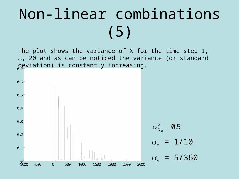
Non-linear combinations (5)
-1000 -500 0 500 1000 1500 2000 2500 30000
0.1
0.2
0.3
0.4
0.5
0.6
0.7Estimated X and its variance
X [km]
P(X
)
The plot shows the variance of X for the time step 1, …, 20 and as can be noticed the variance (or standard deviation) is constantly increasing.
d = 1/10
= 5/360
5.02
0X

Multidimensional Gaussian distributions (1)
)()( 121
21
)2(
1)( XX
TX mxmx
XNX exp
23
22
21
2,31,3
3,21,2
3,12,1
x
x
x
X
xxCxxC
xxCxxC
xxCxxC
The Gaussian distribution can easily be extended for several dimensions by: replacing the variance () by a co-variance matrix () and the scalars (x and mX) by column vectors.
The CVM describes (consists of):
1) the variances of the individual dimensions => diagonal elements
2) the co-variances between the different dimensions => off-diagonal elements
! Symmetric
! Positive definite

MGD (2)
-250 -200 -150 -100 -50 0 50 100 150 200 250-250
-200
-150
-100
-50
0
50
100
150
200
250
X
Y
Un-correlated S.V.
STD of X is 10 times bigger than STD of YSTD of Y is 5 times bigger than STD of X
-250 -200 -150 -100 -50 0 50 100 150 200 250-250
-200
-150
-100
-50
0
50
100
150
200
250
X
Y
Correlated S.V.
STD of X is 10 times bigger than STD of YSTD of Y is 5 times bigger than STD of X
25000
0100)(green
25754287
42877525)(red
19001039
1039700)(green
25000
0100)(red
Eigenvalues => standard deviations
Eigenvectors => rotation of the ellipses
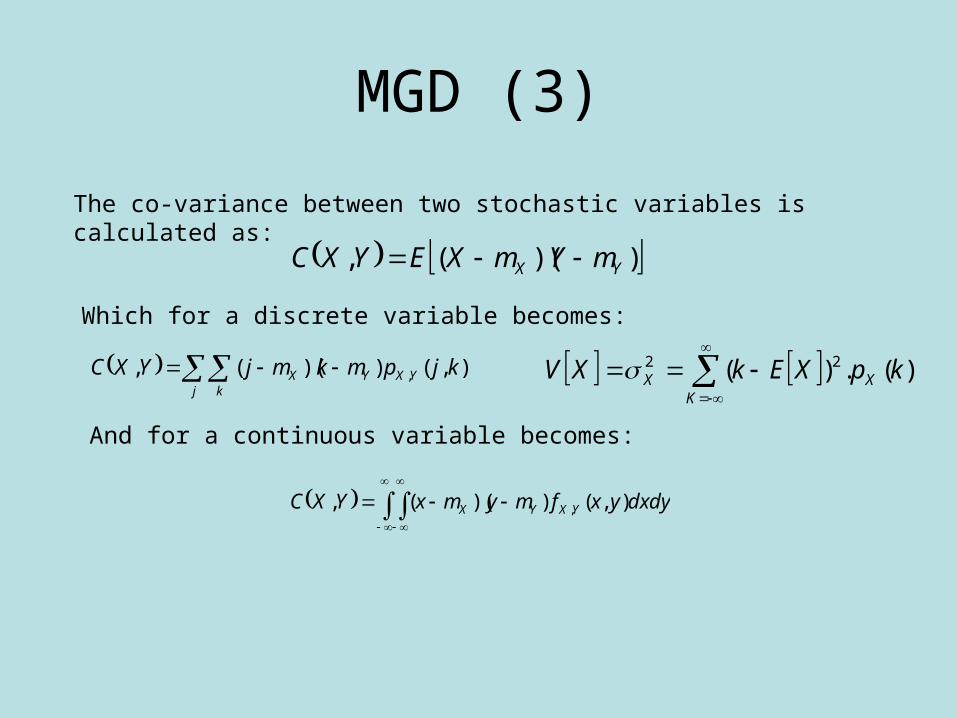
MGD (3)
))((, YX mYmXEYXC
j k
YXYX kjpmkmjYXC ),())((, ,
dxdyyxfmymxYXC YXYX ),())((, ,
The co-variance between two stochastic variables is calculated as:
Which for a discrete variable becomes:
And for a continuous variable becomes:
K
XX kpXEkXV )(.)( 22
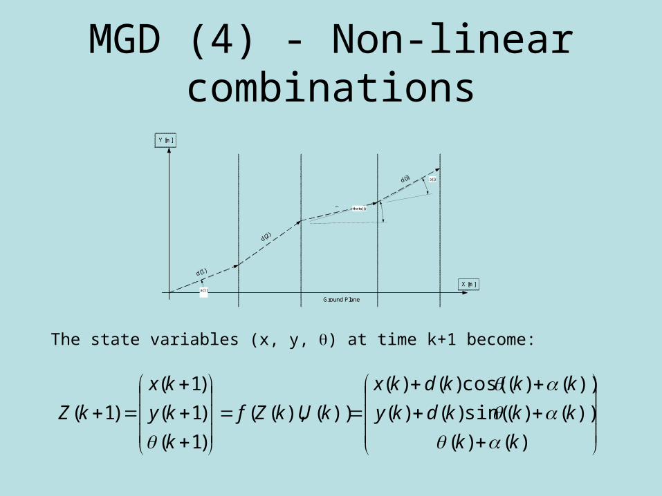
MGD (4) - Non-linear combinations
Ground Plane
a(1)
a(i)
X [m]
Y [m]
theta(i)
)()(
))()(sin()()(
))()(cos()()(
))(),((
)1(
)1(
)1(
)1(
kk
kkkdky
kkkdkx
kUkZf
k
ky
kx
kZ
The state variables (x, y, ) at time k+1 become:

MGD (5) - Non-linear combinations
TUU
TXX fkUffkkfkk )1()|()|1(
)()(
))()(sin()()(
))()(cos()()(
))(),((
)1(
)1(
)1(
)1(
kk
kkkdky
kkkdkx
kUkZf
k
ky
kx
kZ
We know that to calculate the variance (or co-variance) at time step k+1 we must linearize Z(k+1) by e.g. a Taylor expansion - but we also know that this is done by the law of error propagation, which for matrices becomes:
100
))()(cos()(10
))()(sin()(01
kkkd
kkkd
f X
10
))()(cos()())()(sin(
))()(sin()())()(cos(
kkkdkk
kkkdkk
fU
With fX and fU are the Jacobian matrices (w.r.t. our uncertain variables) of the state transition matrix.

MGD (6) - Non-linear combinations
0 200 400 600 800 1000 1200 1400 1600
-200
0
200
400
600
800
1000
Airplane taking off, relative displacement in each time step = (100km, 2deg)
X [km]
Y [
km
]
The uncertainty ellipses for X and Y (for time step 1 .. 20) is shown in the figure.