Minimum Legal Drinking Age and its E�ect on Mortality

Archavanich Kawmongkolsi

March 4, 2015

Abstract

This paper discuss the e�ect of the Minimum Legal Drinking Age(MLDA) and its e�ect on the actual

population that drinks and mortality.Two main datasets will be used, one containing information on the

individual's characteristic and their drinking behavior, while the other contains information on mortality

rate for each cause by age. Since we want to �nd the e�ect from a cuto� or threshold(being over 21), we

will use the Regression Discontinuity Design. After analyzing and using statistical inference, we found

that the MLDA decreases mortality by 8 per 100,000 people.

1 Introduction

The main focus of this paper is to look at the e�ect of Minimum Legal Drinking Age on drinking behavior

and mortality. Many countries have set their MLDA to lower than 21, mostly 18. The reason for this paper

is to see whether or not lowering the MLDA will reduce mortality by reducing alcohol consumption. We

can see the e�ect of the Minimum Legal Drinking Age on drinking rate by looking at whether there is a

jump at the MLDA and estimate how big the jump is. We estimate that MLDA decreases by drinking

rate by 0.078. Using that information we can tie it to the mortality rate for each cause of death on each

age bin to determine the correlation of the MLDA and mortality rate. There are two main datasets used,

the NHIS which contains data on individual's characteristics and drinking habit, and Mortality data which

contains di�erent causes of death for each age. In order to graphically represent the jump in drinking rate

at age 21, a new modi�ed aggregate dataset has to be created. In order to �nd the e�ect of drinking on

1

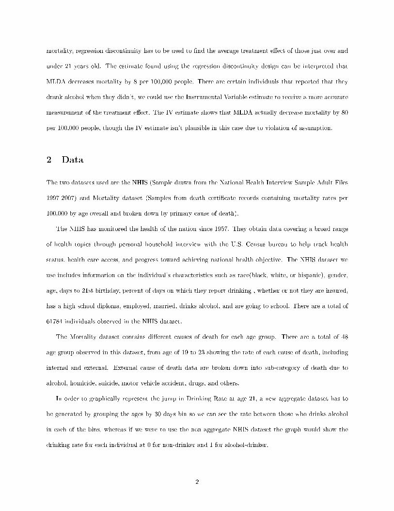
mortality, regression discontinuity has to be used to �nd the average treatment e�ect of those just over and

under 21 years old. The estimate found using the regression discontinuity design can be interpreted that

MLDA decreases mortality by 8 per 100,000 people. There are certain individuals that reported that they

drank alcohol when they didn't, we could use the Instrumental Variable estimate to receive a more accurate

measurement of the treatment e�ect. The IV estimate shows that MLDA actually decrease mortality by 80

per 100,000 people, though the IV estimate isn't plausible in this case due to violation of assumption.

2 Data

The two datasets used are the NHIS (Sample drawn from the National Health Interview Sample Adult Files

1997-2007) and Mortality dataset (Samples from death certi�cate records containing mortality rates per

100,000 by age overall and broken down by primary cause of death).

The NHIS has monitored the health of the nation since 1957. They obtain data covering a broad range

of health topics through personal household interview with the U.S. Census bureau to help track health

status, health care access, and progress toward achieving national health objective. The NHIS dataset we

use includes information on the individual's characteristics such as race(black, white, or hispanic), gender,

age, days to 21st birthday, percent of days on which they report drinking , whether or not they are insured,

has a high school diploma, employed, married, drinks alcohol, and are going to school. There are a total of

61784 individuals observed in the NHIS dataset.

The Mortality dataset contains di�erent causes of death for each age group. There are a total of 48

age group observed in this dataset, from age of 19 to 23 showing the rate of each cause of death, including

internal and external. External cause of death data are broken down into sub-category of death due to

alcohol, homicide, suicide, motor vehicle accident, drugs, and others.

In order to graphically represent the jump in Drinking Rate at age 21, a new aggregate dataset has to

be generated by grouping the ages by 30 days bin so we can see the rate between those who drinks alcohol

in each of the bins, whereas if we were to use the non-aggregate NHIS dataset the graph would show the

drinking rate for each individual at 0 for non-drinker and 1 for alcohol-drinker.

2

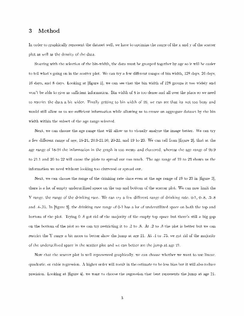
3 Method

In order to graphically represent the dataset well, we have to optimize the range of the x and y of the scatter

plot as well as the density of the data.

Starting with the selection of the bin-width, the data must be grouped together by age so it will be easier

to tell what's going on in the scatter plot. We can try a few di�erent ranges of bin width, 128 days, 26 days,

16 days, and 8 days. Looking at [�gure 1], we can see that the bin width of 128 groups it too widely and

won't be able to give us su�cient information. Bin width of 8 is too dense and all over the place so we need

to restrict the data a bit wider. Finally getting to bin width of 26, we can see that its not too busy and

would still allow us to see su�cient information while allowing us to create an aggregate dataset by the bin

width within the subset of the age range selected.

Next, we can choose the age range that will allow us to visually analyze the image better. We can try

a few di�erent range of age, 18-24, 20.9-21.10, 20-22, and 19 to 23. We can tell from [�gure 2], that at the

age range of 18-24 the information in the graph is too messy and cluttered, whereas the age range of 20.9

to 21.1 and 20 to 22 will cause the plots to spread out too much. The age range of 19 to 23 shows us the

information we need without looking too cluttered or spread out.

Next, we can choose the range of the drinking rate since even at the age range of 19 to 23 in [�gure 2],

there is a lot of empty underutilized space on the top and bottom of the scatter plot. We can now limit the

Y range, the range of the drinking rate. We can try a few di�erent range of drinking rate, 0-1, 0-.8, .2-.8

and .4-.75. In [�gure 3], the drinking rate range of 0-1 has a lot of underutilized space on both the top and

bottom of the plot. Trying 0-.8 got rid of the majority of the empty top space but there's still a big gap

on the bottom of the plot so we can try restricting it to .2 to .8. At .2 to .8 the plot is better but we can

restrict the Y range a bit more to better show the jump at age 21. At .4 to .75, we got rid of the majority

of the underutilized space in the scatter plot and we can better see the jump at age 21.

Now that the scatter plot is well represented graphically, we can choose whether we want to use linear,

quadratic, or cubic regression. A higher order will result in the estimate to be less bias but it will also reduce

precision. Looking at [�gure 4], we want to choose the regression that best represents the jump at age 21.

3

The linear regression

DrinksAlcoholi = β0 + β1posti + β2AgeCenteredi + β3AgeCenteredi ∗ posti + Ui

where post = 1 when age is over 21, and 0 when under 21, best represent the jump. Using this regression

discontinuity design helps us observe near the jump at age 21. Although the results from the linear, quadratic,

and cubic regression are robust; we chose the linear regression because when we compare it with the quadratic

and cubic regression, we can see that there is a large decline in drinking rate as the person approaches age

21 which doesn't make much sense.Our coe�cient of interest is post, since the regression estimate will tell

us the jump in alcohol drinking rate after turning 21.

After �nding the estimate of MLDA on the rate of drinking, we can �nd the estimate of MLDA on

mortality. First we can make a regression table to make sure that the observable characteristic are statistically

insigni�cant documenting that people over 21 and under 21 are very similar using the following regression:

Characteristici = β0 + β1posti + β2AgeCenteredi + β3AgeCenteredi ∗ posti + Ui

The estimates of each regression shows that the co-variates of the two groups (over 21 and under 21) are

similar whether the individual is just over or under 21. Knowing that both the groups are similar will give

us a more legitimate estimate and less bias.

After making sure that the characteristics are similar before and after turning 21, We can visually plot

all the causes of death against the age at the time of death. This will show how much of an e�ect turning

21 has on each causes of death. We run a similar regression based o� the Regression Discontinuity Design:

CauseOfDeath = β0 + β1post+ β2AgeCentered+ β3AgeCentered ∗ post+ Ui

then create a regression table for each cause of death after turning 21 to get an estimate. Our coe�cient of

interest is post, since the regression estimate will tell us the jump in mortality after turning 21.

We can then try using the Instrumental Variable Estimate to get an e�ect of drinking on mortality. The

4

way to �nd Instrumental Variable estimate is to obtain the First Stage and Reduced Form then dividing

reduced form by �rst stage. The reduced form is the e�ect of being assigned to drink alcohol on mortality

The �rst stage is to adjust for those that do not comply to their assignment of drinking/not drinking.

4 Results

Looking at the �tted regression line using the regression discontinuity in [Figure 5] and the estimates in

[Figure 6], we can see that there is a jump in drinking rate after turning 21. In [Figure 5] we can see that

there is a steadily increasing drinking rate leading up to age 21, then the drinking rate jumps up after

turning 21. To see the estimate of the jump we can turn to [Figure 6]. This shows us that under the Linear

Regression Discontinuity, the jump in drinking rate after turning 21 is 0.078. In comparing the Linear vs

Linear with Birthday e�ect model, we can see that all co-variates are signi�cant except for the birthday

e�ect, where the P value is bigger than 0.1. The scatter plot is �ltered for a good visual representation, so it

only shows data grouped together by 26 days from age 19 to 23, and drinking rates of .40 to .75. The linear

regression shows that there is an increase of 0.078 in drinking rate after turning 21.

Next, we can look at [Figure 7] to see from the regression table that of observable characteristics are

statistically insigni�cant, showing us that the characteristics are statistically insigni�cant except for married

which could mean that there may be a large increase of people getting married around age 21, though this

increase will be assumed to not cause further bias on our estimate because certain people may have just

decided to get married right by age 21. The estimates of each regression shows that the co-variates of the

two groups (over 21 and under 21) are similar whether the individual is just over or under 21. Knowing that

both the groups are similar will give us a more legitimate estimate and less bias.

Next, looking at [�gure 8] and [�gure 9], we can see that the jump in all causes of death at age 21

as well as speci�cally to motor vehicle and alcohol death. This could be due to the MLDA being met at

age 21. [�gure 9] estimates that meeting the MLDA increases overall mortality by 8.06 per 100,000 people,

speci�cally motor vehicle accident increases by 3.65 people per 100,000 people and alcohol death increases by

0.37 per 100,000 people with the mortality rate declining as people turns 21. All of the cause of death except

homicide and internal death are statistically signi�cant. homicide and internal death rate being statistically

5

insigni�cant means that these cause of death might not be signi�cantly correlated with turning 21. We use

the robust standard errors for this regression table, because the homoskedasticity assumption is violated.

To account for both compliers and non-compliers, [Figure 10] shows the Instrumental Variable estimates

and standard error for each of the estimates. Looking at the table, the MLDA increases mortality by

79.88 per 100,000. To see if the IV estimates hold, we have to check the following 3 assumptions. 1) The

Instrument(turning 21) is correlated with the endogenous variable(drinking). The �rst assumption holds

because turning 21 is correlated with drinking. 2) Turning 21 is not correlated with the error term. 3)

Turning 21 a�ects mortality only through drinking. Assumption 1 is met as we can see the jump using the

regression discontinuity design. Assumption 2 is questioned since turning 21 could be correlated to some

error terms such in�uence of older friends or dangerous individuals, or transportation to bars and clubs. Due

to the assumptions not being met, the instrumental variable estimates may not be accurate.

5 Conclusion

Starting from creating a graphical representation of both the NHIS and Mortality dataset, we can see that

there is clearly a jump in drinking at age 21 which also a�ects mortality rate. Although we can see the

jump, we have to see if the estimates are accurate starting with internal validity because it directly a�ects

its external validity. Both datasets are reliable as we have checked using the table of regression estimate and

the mortality data are obtained from death certi�cates. We can consider the measurement error in age as

well. The mean 0 measurement error in age is caused when the date gathered in the data aren't exact(only

approximate month and week) due to con�dentiality. This may cause a downward attenuation bias because

people that are just under 21 may be grouped with those over 21 but report that they don't drink. We

can also take reporting error into consideration. Drinking is very under-reported when comparing the data

from surveys to tax records of alcohol being sold. This means the drinking rate might be lower than it

actually is. People that are under 21 may report in surveys that they don't drink, or drink less due to legal

circumstances. This could cause our estimate of the discontinuity to have a downward bias. Many people

who drink alcohol may not be able to remember exactly how many drinks they've had the past week or

months. According to the regression discontinuity design estimate, when the MLDA is met(individual turns

6

21), there is an increase of 8 out of 100,000 mortality. We use the IV to try and get an estimate of the people

that began drinking at age 21 because they are the ones that are driving the increase in mortality estimate.

Since the 3 assumptions does not hold, this means that there are other factors other than those that started

drinking when they turn 21 that is driving the mortality estimate and the IV estimates are invalid. So,

to answer the question of whether or not MLDA reduce drinking and mortality, if so how much? Yes, the

MLDA does reduce drinking and mortality rate by 0.078 and 8.06 per 100,000 people respectively.

7

Figure 1 

 

Figure 2

 

Figure 3

Figure 4 

 

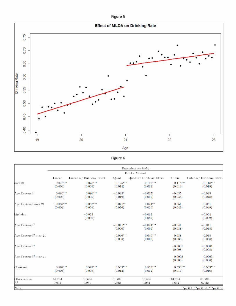
Figure 5 

 

Figure 6 

 

Figure 7 

 

Figure 8 

 

Figure 9 

 

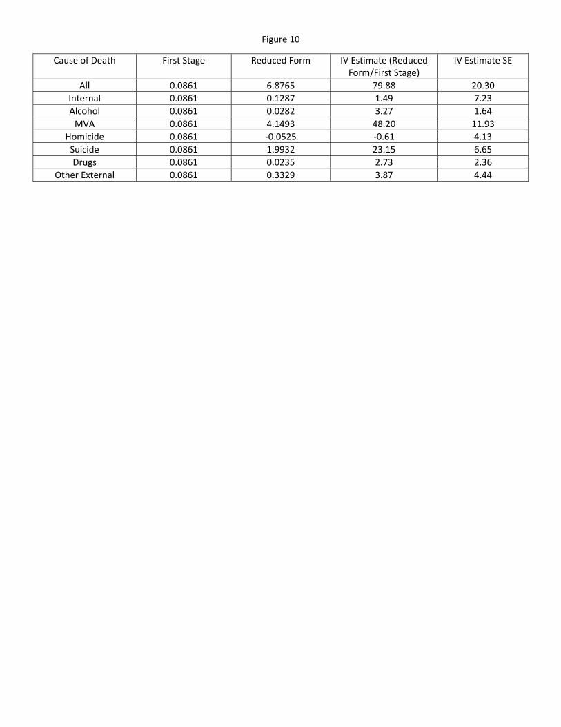
Figure 10 

Cause of Death  First Stage  Reduced Form  IV Estimate (Reduced Form/First Stage) 

IV Estimate SE 

All  0.0861  6.8765  79.88  20.30 

Internal  0.0861  0.1287  1.49  7.23 

Alcohol  0.0861  0.0282  3.27  1.64 

MVA  0.0861  4.1493  48.20  11.93 

Homicide  0.0861  ‐0.0525  ‐0.61  4.13 

Suicide  0.0861  1.9932  23.15  6.65 

Drugs  0.0861  0.0235  2.73  2.36 

Other External  0.0861  0.3329  3.87  4.44