Miren Lafourcade and Giordano Mion Concentration, agglomeration and the size of plants Article (Accepted version) (Refereed)

Original citation: Lafourcade, Miren and Mion, Giordano (2007) Concentration, agglomeration and the size of plants. Regional science and urban economics, 37 (1). pp. 46-68. ISSN 0166-0462 DOI: 10.1016/j.regsciurbeco.2006.04.004 © 2006 Elsevier This version available at: http://eprints.lse.ac.uk/42666/ Available in LSE Research Online: May 2012 LSE has developed LSE Research Online so that users may access research output of the School. Copyright © and Moral Rights for the papers on this site are retained by the individual authors and/or other copyright owners. Users may download and/or print one copy of any article(s) in LSE Research Online to facilitate their private study or for non-commercial research. You may not engage in further distribution of the material or use it for any profit-making activities or any commercial gain. You may freely distribute the URL (http://eprints.lse.ac.uk) of the LSE Research Online website. This document is the author’s final manuscript accepted version of the journal article, incorporating any revisions agreed during the peer review process. Some differences between this version and the published version may remain. You are advised to consult the publisher’s version if you wish to cite from it.

Concentration, Agglomeration and the Size of Plants∗

Miren Lafourcade† Giordano Mion‡

April 27, 2005

Abstract

This paper investigates whether the geographic distribution of manufacturing activities inItaly is likely to differ according to the scale of plants. We find strong evidence of a significantpositive relationship between size and concentration, as in Kim (1995) or Holmes and Stevens(2002, 2004). However, we go one step further in examining how sensitive is this feature to theconsideration of spatial dependence between geographic units. We show that, while large plantsexhibit a clear tendency to cluster within narrow geographical units such as local labor systems,small establishments, by contrast, rather co-locate within wider areas in which a distance-basedpattern emerges. These findings are consistent with plants of heterogeneous size engaging indifferent transport intensive activities.

JEL classification: C21, L11, R12, R30, R34.Keywords: Concentration, Spatial Auto-Correlation, Size of Plants.

∗The authors would like to thank Giuseppe De Arcangelis, Jerome Carreau, Bart Jourquin, Renato Santelia andStefano Usai for their critical help in gathering data, and Antonio Ciccone, Thierry Mayer, Henry Overman, FredericRobert-Nicoud, Fabiano Schivardi, Eric Strobl, Stefano Usai and three anonymous referees for very helpful comments.Mion gratefully acknowledges financial support from the CEPR Research Network on “The Economic Geography ofEurope: Measurement, Testing and Policy Simulations”, funded by the European Commission under the ResearchTraining Network Programme (Contract No: HPRN-CT-2000-00069). The usual disclaimer applies.

†Universite d’Evry (IUT - Departement GLT) and PSE (Paris-Jourdan Sciences Economiques), Unite Mixtede Recherche CNRS-EHESS-ENPC-ENS. PSE, 48 boulevard Jourdan, 75014 Paris, France. lafourca@enpc.fr.http://www.enpc.fr/ceras/lafourcade/.

‡Corresponding author. Universita di Bologna. Dipartimento di Scienze Economiche, Universita di Bologna, str.Maggiore 45, 40125 Bologna, Italy. mion@spbo.unibo.it. http://www.dse.unibo.it/mion/.

1 Introduction

Economists, geographers and historians share a considerable interest in analyzing the causes of

regional specialization. Among the myriad of determinants which have been explored, particular

attention was deserved to regional endowments or raw material intensity, comparative advantages,

localized externalities, or, more recently, transport costs and market potential. In this paper, we

focus on a particular aspect of this complex set of mechanisms, which remains quite unexplored:

the size of plants. Our main contributions are to investigate whether the geographic distribution of

manufacturing activities is related to their establishments’ scope, and to seek for specific distance-

based patterns that could arise from differences in the size of plants.

We address this question by examining Italian census data on manufacturing industries for dif-

ferent years, geographic and industrial scales. By extending the empirical focus on Europe, we thus

hope to complement the seminal empirical studies of Kim (1995) and Holmes and Stevens (2002,

2004), which had both focused on North-American countries. Kim (1995) reports a positive corre-

lation between concentration and both the average plant size per worker and the intensity of raw

materials, across the U.S. manufacturing industries. Holmes and Stevens (2002) find strong support

of the same phenomenon within industries: Plants located in areas where an industry concentrates

are larger, on average, than outside such areas, especially for the manufacturing sector. In addition

to Kim (1995), Holmes and Stevens (2002) emphasize that this positive relationship is robust to the

control of the establishments’ own effects on concentration.

In order to go further in examining the relation between plant size and distribution patterns, we

extend the analytical framework to account for the spatial dependence of geographic units. Recent

papers such as Arbia (2001a), Duranton and Overman (2004) or Marcon and Puech (2003) all point

to significant differences in the patterns of concentration obtained from distance-based measures

conveying the possible propagation of a spatial phenomenon in a continuous space. Accounting for

spatial dependence is therefore important regarding economic policy, as it may alter the picture

of economic density we draw from standard indexes of concentration. Since labor productivity is

positively related to employment density, as shown by Ciccone and Hall (1996) or Ciccone (2002),

examining how densely clustered are the establishments of an industry and how this is likely to

depend upon their employment size, remains high on the police makers’ agenda.

Although our approach builds on this recent revival of spatial dependence, we keep working

with a discrete vision of space as formed by a number of spatial units (which can be more or

less aggregated). This allows us to complement a standard concentration index with an indicator

of spatial association (the Moran index) in order to account for possible spatial auto-correlation

patterns. Spatial auto-correlation is a feature of spatial distribution that has received relatively less

1

attention than concentration and that can be related to transport costs minimization, as supported by

the New Economic Geography literature. Therefore, in the paper, we use the term “agglomeration”

to refer to spatial auto-correlation patterns or, more intuitively, to distance-based clusters that

possibly overlap the boundaries of the geographic units chosen to measure concentration.

We find strong evidence of a non-random positive relationship between size and concentration,

as in Kim (1995) or Holmes and Stevens (2002). Going one step further in examining how sensitive

is such a feature to the consideration of spatial dependence we find that, on average, small plants

exhibit stronger agglomeration patterns. This result suggests that, while large plants would cluster

within narrow geographical units such as local labor systems, small firms, by contrast, would rather

co-locate within wider areas in which a distance-based pattern emerges. One interpretation of these

findings is that the location choices of large Italian plants is less sensitive to domestic distances

and translates into narrow scope dense clusters of activities mainly oriented towards either the local

or the foreign markets. Conversely, small Italian establishments are possibly engaged in transport

intensive activities requiring some proximity to domestic consumers’ markets, which, in return,

would make them more sensitive to national distances than larger establishments. Some exceptions

arise, however, for most of the industries characterizing the so called “Italian Districts”, where

manufacturing activities appear to be extremely concentrated, but only weakly agglomerated, despite

low plant scales.1 We provide several checks showing that these results are robust to changes in

the partition of space and plants, in the industry definition, in the measure of distance, and to

the consideration of industry specific characteristics. Furthermore, as regards the time evolution

of spatial distribution patterns, we find that concentration (agglomeration) has slightly decreased

(increased) over the period 1981-1996, small plants being conducive to more dynamics.

The rest of the paper is organized as follows. Section 2 presents the analytical framework relating

plant scale, industry concentration and industry agglomeration. Section 3 describes the data we use

to investigate the geographic distribution of manufacturing activities in Italy and its dependence to

plant size effects. Furthermore, it discusses briefly how we deal with some well known spatial issues

such as the Modifiable Unit Area Problem (MAUP). Section 4 provides the results of a cross-section

analysis performed for Italian Local Labor Systems and 3-digit manufacturing industries in 1996.

Section 5 checks for the robustness of the results and explores long-run trends. Finally, Section 6

concludes and opens new lines of research.

1This comforts the pertinence of a definition of districts based on two ‘implicit’ criteria: A strong concentration ofplants among which a consistent share of small establishments can be found (Sforzi, 1990), and a production mainlyoriented towards foreign markets (Bagella, Becchetti and Sacchi, 1998).

2

2 Analytical Framework

Various indexes can be used to investigate the regional localization patterns of economic activities.2

A large set of the indexes used by economists, which we refer to as the “concentration” family, splits

space into a certain number of geographic units and seek for relative differences in the number of

activities within each of these units, abstracting from their relative position in space. The second

family of measures, which is generally preferred by geographers, tries to account for the spatial

dependence of regions. We will group this second set of indexes under the “agglomeration” label.

The patterns of regional specialization derived from these two families rarely concur unfortunately.

As both types of indexes present pros and cons, we examine how plant size impacts regional spe-

cialization within an analytical framework combining the two families. This section presents our

“bi-dimensional” framework.

2.1 Measuring concentration

Among the most popular measures of concentration are the location quotient (also known as the

Hoover’s coefficient of localization) and the Gini coefficient. However, such indexes are not directly

appropriate to test for a possible correlation between plant size and concentration: In the case when,

by chance, a location gets a very large plant, a positive correlation would emerge randomly, without

testifying of a real link between concentration and plant size yet.

Although it is possible to adapt such indexes in order to control for random causality, as Holmes

and Stevens (2002) do for the location quotient for instance, a more theory-grounded framework has

been proposed by Ellison and Glaeser (1997) to purge concentration from the own plant size effect.

The measure of concentration we use for Italy builds on their model of location choices.3 Let us

recall briefly the basics of the Ellison and Glaeser’s (1997) model (henceforth EG).4

Let M (S) denote the number of spatial geographic units (sectors), ssi = emps

i/∑M

i=1 empsi the lo-

cation i share of employment in the manufacturing industry s, and xi =∑S

s=1 empsi/

∑Mi=1

∑Ss=1 emps

i

its share of total employment. Henceforth, we omit the industry superscript s, for notation conve-

nience.

The EG approach consists in starting from the employment-based index GEG, equal to GEG =∑M

i=1(si − xi)2, and then in neutralizing for differences in the industrial structure by means of an

2The reader will find in Holmes and Stevens (2004), Combes and Overman (2004), and Fujita, Henderson and Mori(2004), exhaustive presentations of the indexes used in a large set of empirical studies regarding the North-American,European and Asian countries, respectively.

3Many previous empirical studies adopted the Ellison and Glaeser (1997) framework to study the geographic distri-bution of activities. See for instance Maurel and Sedillot (1999) for France, or Devereux, Griffith and Simpson (2004)for the UK.

4Our description of the EG model here builds on the simplified version proposed by Maurel and Sedillot (1999).

3

Herfindahl index of concentration. The EG index obtained derives from a rigorous probabilistic

model of plant location yet. Let N denote the number of plants and z1, ..., zj , ...zN , the shares of

these plants in the total employment of an industry. The fraction of sectoral employment related to

location i is therefore

si =N∑

j=1

zj uji, (1)

where uji = 1 if the business unit j locates in area i, and 0 otherwise. The uji are non-independent

Bernouilli variables such that P (uji = 1) = xi, which means that a random process of plants’ location

choices will, on average, lead to a pattern of employment shares matching the aggregate one (xi), as

well assumed to be exogenous as the size of each plant (zj). More precisely, the authors propose to

model the interaction between the location decisions of any pair of plants j and k belonging to the

same industry by

Corr(uji, uki) = γ for j 6= k, (2)

where γ is a parameter lying between −1 and 1 describing the strength of spillovers within the

industry. In that case, the probability that business units j and k locate in the same area i is

independent upon j and k:

p(i, i) = E[uji uki] = Cov(uji, uki) + E[uji]E[uki] = γxi(1− xi) + x2i . (3)

The probability P that the two plants co-locate in any of the M locations is therefore a linear

function of γ:

P =M∑

i=1

p(i, i) = γ

(1−

M∑

i=1

x2i

)+

M∑

i=1

x2i , (4)

By using data on the location of plants to estimate P , one can thus trace back the parameter γ.

One of the most appealing way to interpret this model is, as suggested by Ellison and Glaeser

themselves, to think about plants as darts thrown in space. Imagine a two-stage process in which

nature first chooses to weld some of the darts into clusters (representing groups of plants that are

sufficiently interdependent that they will always locate together), and then each cluster is thrown

randomly at the dartboard to choose a location. The importance of spillovers is then captured by

the parameter γ, which can be viewed as the “fraction” of plants among which co-location occurs.

Ellison and Glaeser (1997) propose the following un-biased estimator of γ

γEG =

GEG

1−M∑

i=1x2

i

−H

1−H, (5)

4

where H =∑N

j=1 z2j is an Herfindahl index controlling simultaneously for industrial differences in

both the number and size of plants.

2.2 Concentration and the size of plants

The EG index allows one to compare geographic concentration across industries because it is immune

to biases arising from differences in their establishment structure. However, the EG location model

neglects the possible occurrence of a correlation between plant size and concentration, as, within

each industry, the probability p(i, i) for two plants to co-locate is independent upon their size. In

the same spirit as in Holmes and Stevens (2002), a simple argument can be used to test for a non

random relation between concentration and the size of plants, however: In a world where the size of

establishments would be independent on concentration patterns, all the variability in the geographic

distribution of manufacturing activities should equally reflect differences in the number of plants.

By comparing the EG employment-based measure of concentration to its plant-based counterpart,

whose properties have been studied by Maurel and Sedillot (1999), one can therefore exhibit possible

discrepancies arising from differences in the scale of plants. As far as both the employment-based

and plant-based estimators are equivalent under the null of a random link between concentration

and size, but still different under the alternative, one can relate the differences arising under this

alternative to the size of plants in each industry. The plant-based estimator proposed by Maurel

and Sedillot (1999), henceforth labeled “un-weighted” (UW) because it treats all observations the

same, is

γUW =

GUW

1−M∑

i=1x2

i

− H

1− H, (6)

where GUW =∑M

i=1

(niN

)2 − ∑Mi=1 x2

i and niN , the share of plants located in i. The Herfindahl

H = 1/N , which accounts for differences in the number of plants, is the counterpart of the one used

in the employment-based EG index.

Maurel and Sedillot (1999) proved that this plant-based index of concentration is also an un-

biased estimator of the spillover parameter γ. Furthermore, it is easy to show that γUW is more

efficient than its employment-based counterpart γEG.5

Significant data discrepancies between γUW and γEG testify of a non random relationship between

plant size and location choices. Indeed, if one relaxes the assumption that the tendency for plants to

concentrate would not depend upon the establishment scale, then the EG and UW estimates should

depart significantly one from the other. The EG index would actually reflect the concentration of

5Like in the standard linear regressions framework, both a weighted and an un-weighted estimator are un-biasedbut, if there is no heteroscedasticity, the latter should have a smaller variance.

5

large plants, while the UW counterpart would be more illustrative of small plants (whose number is

much larger).

We now turn to the issue of spatial auto-correlation and its link with the size of plants.

2.3 Measuring agglomeration

The picture we draw from a partition of space into isolated grids is likely to be altered by the

consideration of spatial linkages between grids. Let us illustrate the role of spatial dependence with

an example inspired from Arbia (2001b), in which we consider the distribution of 12 plants over the

9 locations embodied in the cells of a 3x3 grid.

Figure 1: Agglomeration or concentration?

a b

3 3

3 3

3

3 3

3

In Figure 1, the uneven distribution of activities results in two different spatial configurations.

One (case b) is concentration, which can be referred to as a concept of variability that is not sensitive

to the permutation of observations in space. Indicators such as the location quotient, the Gini

coefficient, or even the γEG and γUW estimators, actually measure spatial concentration because

they give a quantification of how much a phenomenon presents spatial variability with respect to

some average. However, they treat data without considering their relative position in space (i.e.

they do not consider distances between spatial units), so that their value would be the same in both

the cases a and b of Figure 1. By contrast, the other configuration (case a) reflects agglomeration6

because it testifies of a certain degree of spatial dependence, which translates into the left corner

distance-based cluster among observations. More precisely, there is spatial auto-correlation as long

as, for each industry, knowing the location of plants in region i is ‘linearly’ informative about the

location of the other plants of the same industry in neighboring regions.

In order to capture the spatial phenomenon of agglomeration, very accurate indexes have been

developed. Among such indicators are the statistics proposed by Cliff and Ord (1981), Getis and

Ord (1992), or Moran (1950), the latter being the one we actually use in this paper. Define first a

6The exact terminology used by Arbia (2001b) is actually “polarization”. However, we prefer “agglomeration”because it is the term that is now widely used in the field of New Economic Geography (NEG) to actually reflect thelocation process arising from the interaction between transport costs (and so distance) and increasing returns to scale.For a comprehensive review of NEG theoretical frameworks, see Fujita, Krugman and Venables (1999) or Fujita andThisse (2002).

6

M×M spatial weighting matrix W , as the matrix whose generic element wil is the relative weight of

location l for location i and wii = 0. wil may either rely on simple contiguity criteria (for instance,

a first-order contiguity matrix will give weight one to all contiguous locations and zero otherwise,

including the own location), or be inversely related to the distance dil between i and l (under various

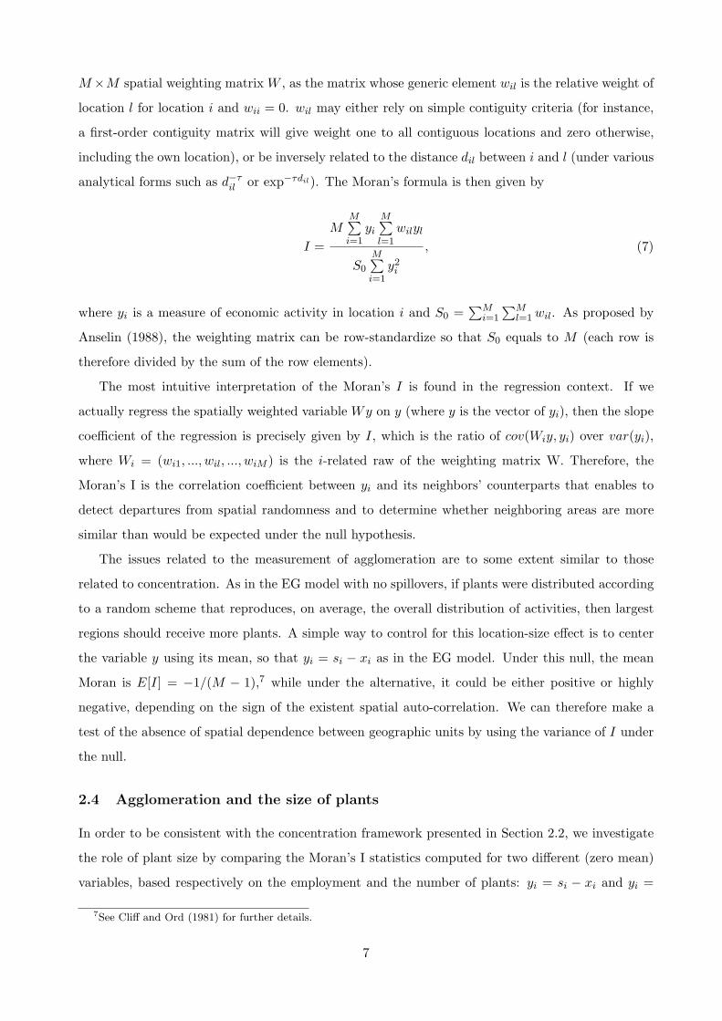
analytical forms such as d−τil or exp−τdil). The Moran’s formula is then given by

I =M

M∑i=1

yi

M∑l=1

wilyl

S0

M∑i=1

y2i

, (7)

where yi is a measure of economic activity in location i and S0 =∑M

i=1

∑Ml=1 wil. As proposed by

Anselin (1988), the weighting matrix can be row-standardize so that S0 equals to M (each row is

therefore divided by the sum of the row elements).

The most intuitive interpretation of the Moran’s I is found in the regression context. If we

actually regress the spatially weighted variable Wy on y (where y is the vector of yi), then the slope

coefficient of the regression is precisely given by I, which is the ratio of cov(Wiy, yi) over var(yi),

where Wi = (wi1, ..., wil, ..., wiM ) is the i-related raw of the weighting matrix W. Therefore, the

Moran’s I is the correlation coefficient between yi and its neighbors’ counterparts that enables to

detect departures from spatial randomness and to determine whether neighboring areas are more

similar than would be expected under the null hypothesis.

The issues related to the measurement of agglomeration are to some extent similar to those

related to concentration. As in the EG model with no spillovers, if plants were distributed according

to a random scheme that reproduces, on average, the overall distribution of activities, then largest

regions should receive more plants. A simple way to control for this location-size effect is to center

the variable y using its mean, so that yi = si − xi as in the EG model. Under this null, the mean

Moran is E[I] = −1/(M − 1),7 while under the alternative, it could be either positive or highly

negative, depending on the sign of the existent spatial auto-correlation. We can therefore make a

test of the absence of spatial dependence between geographic units by using the variance of I under

the null.

2.4 Agglomeration and the size of plants

In order to be consistent with the concentration framework presented in Section 2.2, we investigate

the role of plant size by comparing the Moran’s I statistics computed for two different (zero mean)

variables, based respectively on the employment and the number of plants: yi = si − xi and yi =

7See Cliff and Ord (1981) for further details.

7

(niN

)− xi. We therefore obtain the two following measures of agglomeration:

IW =(M/S0)

M∑i=1

(si − xi)M∑l=1

wil (sl − xl)

M∑i=1

(si − xi)2

and IUW =(M/S0)

M∑i=1

(niN − xi

) M∑l=1

wil

(nlN − xl

)

M∑i=1

(niN − xi

)2,

(8)

For these two Moran indexes, we face an issue similar to that of the concentration framework. In

order to perform comparisons between sectors, we have to consider that extreme agglomeration may

occur because, in some industries, only a very small number of plants operate in comparison with

the number of locations. For such industries, strong positive auto-correlation may thus testify of

emptiness surrounded by emptiness. As the consideration of neighboring empty locations may lead

to over-estimate the true number of industrial clusters, we will actually check whether the correlation

identified between agglomeration and plant size is not triggered by industries with an extremely low

numbers of plants.

A specific issue, to which concentration indexes are immune, and which is thus inherent to the

Moran index, arises from its regression coefficient nature. As in all regression contexts, the presence

of outliers in the sample may bias the Moran indicator towards an agglomeration tendency that

is not representative of the majority of observations. In order to not over-estimate the degree of

spatial auto-correlation, Anselin (1995) proposes an identification procedure based on a conditional

randomization approach. For each location i, Anselin (1995) suggests first to compute a local Moran

statistic, Ii, measuring the correlation between a particular yi and its specific neighbors, and then

to make a test of its local instability. Furthermore, as the Moran index corresponds to the sample

average of the I ′is, he also suggests to use the sample variance of the I ′is to identify the outliers on

a two-sigma rule basis. The locations that emerge as extreme values with both tests are actually

spatial outliers or, borrowing the terminology of Anselin (1995), “hot spots”. The reason for this

double check is the need to test for local instability when the null is not randomization, but some

degree of spatial correlation. Under spatial correlation indeed, the presence of outliers is more likely

to occur than under a random scheme. We will thus pay particular attention to identify and analyze

these “hot spots”, in order to be sure that the agglomeration indexes obtained are representative

of the majority of industrial observations and provide a robust measure of the correlation found

between agglomeration and plant size.

8

3 Data and methodological issues

We use data from the Italian Census of economic activities, which gives information on the location

and employment of the universe of Italian plants. This data set is very detailed in its geographic

coverage of manufacturing industries. The geographic scale of observation can be disaggregated up

to the 8192 Italian commons and the industrial scale up to the 3-digit NACE nomenclature (revision

1) for the years 1981 and 1991, and to the 5-digit category counterpart for 1996.

Contrary to most of the previous empirical studies investigating the geographic distribution of

activities (as Ellison and Glaeser, 1997, Maurel and Sedillot, 1999, or Holmes and Stevens, 2002 and

2004), there is no problem of withheld data in this sample, the only limitation being that, in some

cases, the size of plants had to be recovered from the size-range groups to which data are allocated.

Nonetheless, it is important to notice that, given the high level of data disaggregation, in roughly

90% of the cases, the size of plants was directly identified and not estimated. Moreover, information

on the size of plants is not necessary to obtain γUW and IUW , which are less demanding than γEG

and IW .

3.1 Partitioning space and industries

To apply both the concentration and agglomeration indexes, we have first to choose an adequate

scale of industry aggregation and an appropriate geographic unit of analysis.

As recalled by Kim (1995), the definition of industry aggregation depends on the subjacent

phenomena one is willing to understand through the geographic distribution of activities. Indeed,

industrial spillovers and the incentives for plants to co-locate can either operate within a narrowly

defined category of industries such as the 3-digit nomenclature of activities, or a more broadly defined

category such as the 2-digit nomenclature. As regards the Italian census, the 3-digit category leads to

study 103 different sub-activities within the manufacturing industry, whereas the 2-digit counterpart

would divide the latter in only 23 sub-industries. In the case of Italy, the 3-digit category makes

more salient the industries that gave birth to some well-known districts, such as ‘Preparation and

spinning of textile fibres’ (3-digits NACE number 171), ‘Textile weaving’ (172), ‘Tanning and dressing

of leather’ (191), ‘Watches and Clocks’ (335), ‘Manufacturing of Musical instruments’ (363), or

‘Ceramic tiles and flags’ (263). Although we will put the emphasis on the results obtained under the

finest level of industrial disaggregation to account for the district phenomenon, we will also use the

information provided by the sample of 2-digit activities to check for the robustness of the results to

a change in the industry partition.

The second issue we have to tackle is the Modifiable Unit Area Problem (henceforth MAUP),

which arises from partitioning space into an arbitrary number of geographic units. The problem,

9

which is very well documented in Arbia (1989 and 2001b), concerns both the boundaries and the

scale chosen. It can be illustrated as follows:

Figure 2: The MAUP problem

c d

6 3

3

12

As apparent from Figure 2, one can see that, by enlarging the grid of squares of Figure 1 in an

asymmetric way, we may alter the picture of both agglomeration and concentration. Figure 2 leads to

the exactly reverse configuration than that observed in Figure 1: Case c, which is the counterpart of

case a, now reflects pure concentration, whereas case d, which is the counterpart of case b, embodies

agglomeration.

The first precaution we take to minimize the MAUP is to choose a partition of space that relies

on real economic features. The partition we adopt is the one of Local Labor Systems (henceforth

LLS). The LLS spatial nomenclature, which covers both urban and rural areas, divides the Italian

territory into 784 geographic units. The average LLS spreads over 384 km2, which is equivalent to

splitting the U.S. continental territory into more than 25,000 units. Therefore, the LLS grid is not

far from being equivalent to the U.S. partition into 41,313 zip-code units. The boundaries of LLS

were defined in 1991 by the Italian Statistic Institute on the basis of minimum daily commuting

patterns, so as to maximize the correspondence between the people living and working areas. The

geographic scale of LLS is therefore much less arbitrary than a more standard partition based on

simple administrative schemes.

Although the core of the paper will focus on LLS only (Section 4), we will be cautious in that the

distribution patterns obtained for LLS do not hold only for this specific partition scheme. In section 5,

we will thus check for the robustness of the results to the adoption of a more aggregated partition

of space. We choose the NUTS3 scale of aggregation (Italian “provincie”), which splits the Italian

territory in 95 geographic units. Checking for the robustness of the results to a thinner partition

of space than LLS - which, as recalled, is already very disaggregated as it is almost equivalent to a

partition of the U.S. space into zip-codes - would certainly warrant consideration. However, since

disaggregating further the geographic scale would reduce computational practicality and lead to

extremely heavy calculations,8 we investigate the issue of considering wider geographic units only.

8A disaggregation into the 8192 municipalities, for instance, requires to treat 103 x 8192 = 843,716 industry-space

10

3.2 Partitioning the universe of plants

In order to explore the role of plant heterogeneity, we must partition the universe of establishments

into at least two groups: Large and small. However, defining a clear frontier between the two is

far from being trivial. As in Holmes and Stevens (2002), pragmatism leads us to adopt the simple

strategy of cutting the sample of plants according to their number of employees. The choice of an

employment threshold is obviously arbitrary, but knowing the features of Italian labor markets is

helpful in reducing such arbitrariness. Regarding the employment legislation in Italy, two minimum

cut-off values arise naturally.

A first threshold of 20 workers makes sense regarding both the fiscal and legal status of Italian

firms. Indeed, Italian firms with less than 20 workers (“piccole imprese”) benefit from specific

incentives such as tax credits, or lower social contributions and loan interest rates. Furthermore, in

order to have an employee board a firm must have at least 20 employees. Finally, this 20 employees

cut-off, which has been also chosen by Holmes and Stevens (2002) for the U.S., offers an interesting

comparison perspective, on top of being the only threshold that is compatible with the 1981 and

1991 older census data. Table 1 exhibits summary statistics for the two sub-samples obtained when

partitioning the universe of Italian plants according to the more or less than 20 workers scheme. As

apparent from Table 1, the threshold of 20 matches nearly the median plant, which actually comforts

its judiciousness regarding a dichotomic partition scheme.

Table 1: Summary Statistics on the 20-workers partition of Italian plants.

Sample of small plants Sample of Large plantsMean size 3.73 67.84St. deviation 11.26 222.18Coefficient of variation 3.02 3.27Number of manuf. plants 549,747 41,363% of manuf. plants 93.01 6.99% of manuf. employment 42.20 57.80

However, a second minimum threshold of 15 workers is more pertinent as regards the Italian

dismissing law.9 Indeed, when a dismissal is judged illegal, a worker has the right to be reintegrated

in the firm if the latter is larger than 15 employees, otherwise he is entitled to receive a monetary

compensation. This distinction actually turns out to be crucial as regards labor costs because it

favors smaller units. Furthermore, the 15 employees threshold is used by the Italian legislation with

reference to many other labor and fiscal issues such as working overtime, disabled’s hiring, training,

or tax benefits.

observations, meaning that the calculation of indexes is not feasible under reasonable delays.9See “Statuto dei Lavoratori” art. 18.

11

Although the first cut-off of 20 is preferable in terms of cross-studies and cross-time comparisons,

the second one seems more reasonable from a legal point of view. We will concentrate first on the

20-workers partition scheme (Section 4) and then turn to robustness checks. As the distribution of

employment is more detailed in 1996 than in 1981 and 1991, we will check in Section 5 whether

the 1996 results are robust to the threshold chosen (15 vs 20) and the dichotomic partition scheme

adopted (small/large vs small/medium/large plants).

3.3 Measures of distance and weighting matrix

In order to compute the Moran statistic, we need a spatial weighting matrix. Following Harris (1954)

and the large strand of gravity estimations recently surveyed by Disdier and Head (2005), we use

the inverse of bilateral distance to measure the spatial interdependence of LLS.10 The only measure

of distance available at the very disaggregated scale of LLS is the great-circle distance.11 Section 4

will thus report the agglomeration indexes derived from the implementation of this linear-distance

based matrix.

However, we have to be cautious in that the geographic scope of agglomeration is likely to depend

upon effective rather than linear distance. For instance, if mountainous relief impedes one to access

a location, as it might be the case in the Italian Alps, the firms may prefer to locate elsewhere.

Likewise, the configuration of real transport networks may also affect the firms’ location choices.

In order to guarantee fast delivery and implement “just-in-time” practices for instance, plants may

prefer to locate alongside highways, as illustrated for instance in Arbia (2001a) for the San Marino

Republic. Unfortunately, an effective measure of distance is not available at the scale of Italian LLS,

which is too thin. However, real distances can be computed at the more aggregated geographic scale

of the 95 Italian provinces, and we will use them in Section 5 to check for the robustness of our

results. The calculation of effective bilateral distances builds on an original GIS provided by Bart

Jourquin, that we implement on the TRIPS transport modelization software. This association allows

us to extract the distance related to the fastest itinerary connecting any pair of Italian provinces

through the real road transport network in 1996.12

10In Lafourcade and Mion (2003), we also experiment first-order contiguity matrices, but as the results obtained arequalitatively similar, we do not report them.

11The great-circle distance is the shortest bilateral distance between the centroids of two geographic units, assumingthey would be on a sphere without any physical or network constraint between them. The average great-circle distancebetween Italian LLS is 467 km.

12For more details on the methodology, see Combes and Lafourcade (2005).

12

4 Basic Results for Italy: LLS, 3-digit industries, 1996

To explore the impact of plant size on the geographic distribution of activities, Section 4.1 first

compares the concentration and agglomeration indexes computed on both an employment and a

number of plants basis. Section 4.2 seeks for the role of plant size heterogeneity in explaining the

large discrepancies found within industries. Section 4.3 ends with a cross-industry comparison of

the influence of plant size.

4.1 Discrepancies between the employment- and plant-based indexes of concen-

tration and agglomeration

As apparent from Table 2, one can see that the correlation between the employment- and plant-based

measures of both the concentration and the agglomeration measures is quite weak.

Table 2: Concentration and agglomeration indexes (784 LLS): All plants.

Concentration AgglomerationγEG γUW IW IUW

Average value 0.033 0.022 0.010 0.018Average st. deviation 0.0115 0.0018 0.0025 0.0031R2 0.20 0.60R2 ranks 0.54 0.67Number of manuf. plants 591,110 591,110Number of industries 103 103Number of spatial units 784 784

See Appendix B for detailed results on the 103 3-digit industries.

As regards concentration, both the weighted and un-weighted indexes suggest that Italian man-

ufacturing activities are strongly concentrated. Based on a two-sigma rule criterion,13 γEG (γUW )

are significantly different from zero in 91% (97%) of the industries.14 However, the average weighted

estimator is 50% larger than its un-weighted counterpart and we estimate that around 60% (25%)

of the industries exhibit a significant positive (negative) differential.15 Such discrepancies are very

large and suggest that concentration is significantly stronger for large establishments (that are over-

weighted in the employment-based indexes) than for small ones. The difference in average standard

13The difference between the index and its expected value under the null of no spillovers (zero) has to be larger thantwice its standard deviation for an industry to be concentrated.

14Ellison and Glaeser (1997) define the degree of concentration by classifying industries on a scale referring to boththe mean and median γ. They find that 25% of the U.S. manufacturing industries are highly concentrated, while50% testify of slight concentration only. The Maurel and Sedillot (1999) and Devereux, Griffith and Simpson (2004)counterpart values are respectively, 27% (for France) and 16% (for the UK) of highly concentrated industries, againstrespectively 50% (for France) and 65% (for the UK) of slightly concentrated ones. Our results lead to the sameconcentration ranges for Italy.

15The variance of γEG and γUW is available only under the null of no spillover effect (γ = 0), so that it is not possibleto properly test the differences between two positive values of the estimators. However, assuming normality, we canuse the variances to perform a test based on twice the sum of the standard deviations.

13

errors is also important, with a magnitude so strong (up to 15 times) that this is suggestive of a

strong un-accounted heterogeneity in the sample of plants. Furthermore, correlations between the

weighted and un-weighted concentration indexes are very weak, for both the values and ranks.

As regards agglomeration, a two-sigma rule criterion16 leads to the result that 66% (86%) of the

industries exhibit a significant tendency to be agglomerated according to IW (IUW ). Such features,

which are reminiscent of the trends found by Usai and Paci (2002), testify of the crucial role played by

spatial dependence in the location of manufacturing plants. As for discrepancies among the indexes,

the average un-weighted Moran is 80% larger than its weighted counterpart, the difference being

significantly positive (negative) for around 55% (5%) of the industries. This difference comforts the

evidence of the sample heterogeneity already found for concentration indexes. Finally, one can notice

that the correlations found between the weighted and un-weighted agglomeration indexes, despite

being much larger than their concentration counterparts (for both values and ranks), are not as high

as what would be expected from location choices that would not depend upon the size of plants.

Discrepancies between employment- and plant-based indexes of both concentration and agglom-

eration are therefore large. What is the source of such heterogeneity? Next section puts the emphasis

on the role of plant size in explaining such differences.

4.2 Large vs small plants: Within-industry comparisons

Table 3 disentangles the calculation of concentration and agglomeration indexes between plants with

less than and at least 20 employees.

Table 3: Concentration and agglomeration indexes (784 LLS): Small vs large plants

Sample of small plants Sample of large plantsConcentration Agglomeration Concentration AgglomerationγEG γUW IW IUW γEG γUW IW IUW

Average value 0.024 0.022 0.016 0.018 0.036 0.033 0.007 0.009Average st. deviation 0.0016 0.0010 0.0029 0.0032 0.0047 0.0020 0.0024 0.0025R2 0.90 0.89 0.81 0.70R2 ranks 0.92 0.85 0.73 0.72Number of manuf. plants 549,747 549,747 41,363 41,363

See Appendix B for detailed results on the 103 3-digit industries.

In both cases, the correlation between the weighted and the un-weighted indexes is now quite

good, suggesting that, once controlled for the heterogeneity of plant size, the employment- and

plant-based indicators become data consistent. This is particularly true for the sub-sample of small

establishments for which this correlation amounts to as much as 0.90, for both the concentration and

16The difference between the Moran and its expected value under the null (-1/(M-1)) has to be larger than twice itsstandard deviation for an industry to be agglomerated.

14

agglomeration indexes. The relatively higher correlation found for small plants can be attributed to

the larger homogeneity of the related sample. For the sample of large plants, the ratio between the

smallest and the biggest business unit is around one hundred indeed, which is much higher than 19.

Moreover, differences in the average indexes reduce drastically, in all cases. Finally, the evidence

of a clear non-random relation between the geographic distribution of manufacturing activities and

the size of plants is further supported by a strong reduction in the data variability when splitting

the sample. For instance, while the un-weighted concentration estimator has a lower variance,

coherently with the underlying EG model, the magnitude of the difference is now compatible with a

simple efficiency problem rather than with a plant size heteroscedasticity issue.

Once it is recognized that the partition into small and large units gives coherent results inde-

pendently on the particular index used, it seems reasonable to evaluate different concentration and

agglomeration patterns based on different plant sizes. Comparing the samples of large and small

plants, it is straightforward to see that plant-based concentration indexes are around 50% larger for

large than for small establishments. More precisely, with a two-sigma rule on γUW , we find that, in

60% of the industries, large plants are significantly more concentrated than small ones. The converse

is true only in 26% of the industries. Holmes and Stevens (2002) find comparable results for the

U.S.: The EG index for plants belonging to the fourth quartile (268 employees on average) is found

to be twice larger than its first quartile counterpart (25 employees on average). Our results there-

fore support the non-random positive relationship between size and concentration already found by

Holmes and Stevens (2002) for the U.S. or by Barrios, Bertinelli and Strobl (2003) for Ireland.

However, as one can also notice, small plants exhibit stronger agglomeration patterns than large

establishments, on average. The mean I is actually 2-3 times larger when computed for the sample of

small plants than for its counterpart. Moreover, applying a two-sigma rule on IUW reveals that small

plants are significantly more (less) spatially correlated than large ones in 52% (9%) of industries.

Small plants thus seem to be more sensitive to distance-based patterns. Furthermore, although

the evidence of agglomeration weakens when we exclude the spatial outliers identified with the

methodology of Anselin (1995), the result that the distribution of smaller firms is characterized by

a higher spatial correlation still holds. This feature, which is thus robust to the exclusion of “hot

spots”, suggests that, while large plants would locate within narrow geographical units such as local

labor systems, small firms, by contrast, would rather distribute into wider distance-based clusters.

Measures of concentration and agglomeration therefore strongly depend upon differences in the

size of plants within industries. In Section 4.3, we provide cross-industry comparisons based on

extreme patterns of concentration and agglomeration in order to highlight the following question:

Relying on plant size characterization of concentration and agglomeration, what could be the un-

15

derlying mechanisms governing the spatial distribution of activities? This issue is likely to be an

important topic as regards the design of regional development policies.

4.3 Large vs small plants: Between-industry comparisons

Tables 4 and 5, derived from the detailed 3-digit LLS results presented in Tables 13, 14, and 15 in

Appendix B, report the ten manufacturing industries displaying the largest and lowest indexes of

concentration and agglomeration. As the distinction between the un-weighted and weighted indexes

is no longer an issue once corrected for the heterogeneity of plant size, the following results build on

the un-weighted indexes only, because of efficiency properties.

Table 4: The 10 most concentrated and agglomerated industries (784 LLS): Sample of small plants

The 10 more concentrated The 10 more agglomerated

NACE 3-digits industry γUW NACE 3-digits industry IUW

172 Textile weaving 0.247 154 Mauf. of vegetable and animal oils and fats 0.125171 Preparation and spinning of textile fibres 0.244 153 Process. and preserving of fruit and vegetables 0.104191 Tanning and dressing of leather 0.204 158 Manuf. of other food products 0.082296 Manuf. of weapons and ammunition 0.164 232 Manuf. of refined petroleum products 0.075263 Manuf. of ceramic tiles and flags 0.117 266 Manuf. of articles of concrete, plaster and cement 0.073192 Manuf. of handbags, saddlery, harness 0.067 281 Manuf. of structural and metal products 0.059244 Manuf. of pharmaceuticals, med. chemicals, etc. 0.065 193 Manuf. of footwear 0.059173 Finishing of textiles 0.061 203 Manuf. of uilders’ carpentry and joinery 0.057160 Manuf. of tobacco products 0.059 265 Manuf. of cement, lime and plaster 0.051363 Manuf. of musical instruments 0.049 287 Manuf. other fabricated metal products 0.047

See Appendix B for detailed results on all the 103 3-digit industries.

Table 5: The 10 most concentrated and agglomerated industries (784 LLS): Sample of large plants

The 10 more concentrated The 10 more agglomerated

NACE 3-digits industry γUW NACE 3-digits industry IUW

223 Reproduction of recorded media 0.393 153 Process. and preserving of fruit and vegetables 0.047191 Tanning and dressing of leather 0.219 193 Manuf. of footwear 0.039296 Manuf. of weapons and ammunition 0.216 160 Manuf. of tobacco products 0.038263 Manuf. of ceramic tiles and flags 0.172 334 Manuf. of optical instruments, photo. equipment 0.034355 Manuf. of other transport equipment 0.170 363 Manuf. of musical instruments 0.029363 Manuf. of musical instruments 0.155 152 Process. and preserving of fish products 0.028362 Manuf. of jewelery and related art 0.129 182 Manuf. of other wearing apparel and accessories 0.027173 Finishing of textiles 0.089 295 Manuf. of other special purpose machinery 0.026221 Publishing 0.079 232 Manuf. of refined petroleum products 0.025244 Manuf. of pharmaceuticals, med. chemicals, etc. 0.078 293 Manuf. of agricultural and forestry machinery 0.022

See Appendix B for detailed results on all the 103 3-digit industries.

16

A first striking feature arising from the comparison of Tables 4 and 5 is that extreme concentration

and agglomeration patterns are triggered by different industries.

Among the most significantly concentrated industries emerge the activities which are at the

core of Italian districts: ‘Preparation and spinning of textile fibres’ (3-digit NACE number 171)

and ‘Textile weaving’ (172) located in the ‘Prato’ LLS, ‘Tanning and dressing of leather’ (191) in

both the LLS of ‘Arzignano’ and ‘Santa Croce’, ‘Ceramic tiles and flags’ (263) around the LLS of

‘Sassuolo’, ‘Manufacturing of jewelery and related articles’ (362) in the LLS of Alessandria’, ‘Arezzo’

and ‘Vicenza’, and ‘Manufacturing of Musical Instruments’ (363) in the LLS of ‘Ancona’.17 The

districts related to textile industries (171, 172) exhibit an extreme concentration mainly triggered

by small firms (less than 20 employees), while the concentration of other districts seem to be more or

less equally conveyed by small and large plants (191, 263, 363). These features are therefore coherent

with a rough characterization of Italian districts according to their large proportion of small plants,

as in Sforzi (1990). Interestingly, while being so concentrated, industries behind the formation of

districts are only weakly or sometimes not agglomerated at all, as shown by the non significance of

either the weighted or the un-weighted Moran indexes. Despite particularly low plant scales, Italian

districts would stem as an exception to the overall trend that small plants would locate according

to wide national distance-based patterns. This apparently puzzling feature can be attributed to the

fact that the production of many Italian districts is mainly oriented towards foreign markets, as

emphasized by Bagella, Becchetti and Sacchi (1998).

However, a clear exception to this story arises for the ‘Manufacturing of Musical Instruments’,

which is the only district industry that is simultaneously extremely concentrated and agglomerated,

independently on the size of its related plants (the industry 363 is present in nearly all columns of

Tables 4 and 5). However, complete separation can be restored by showing that the agglomeration

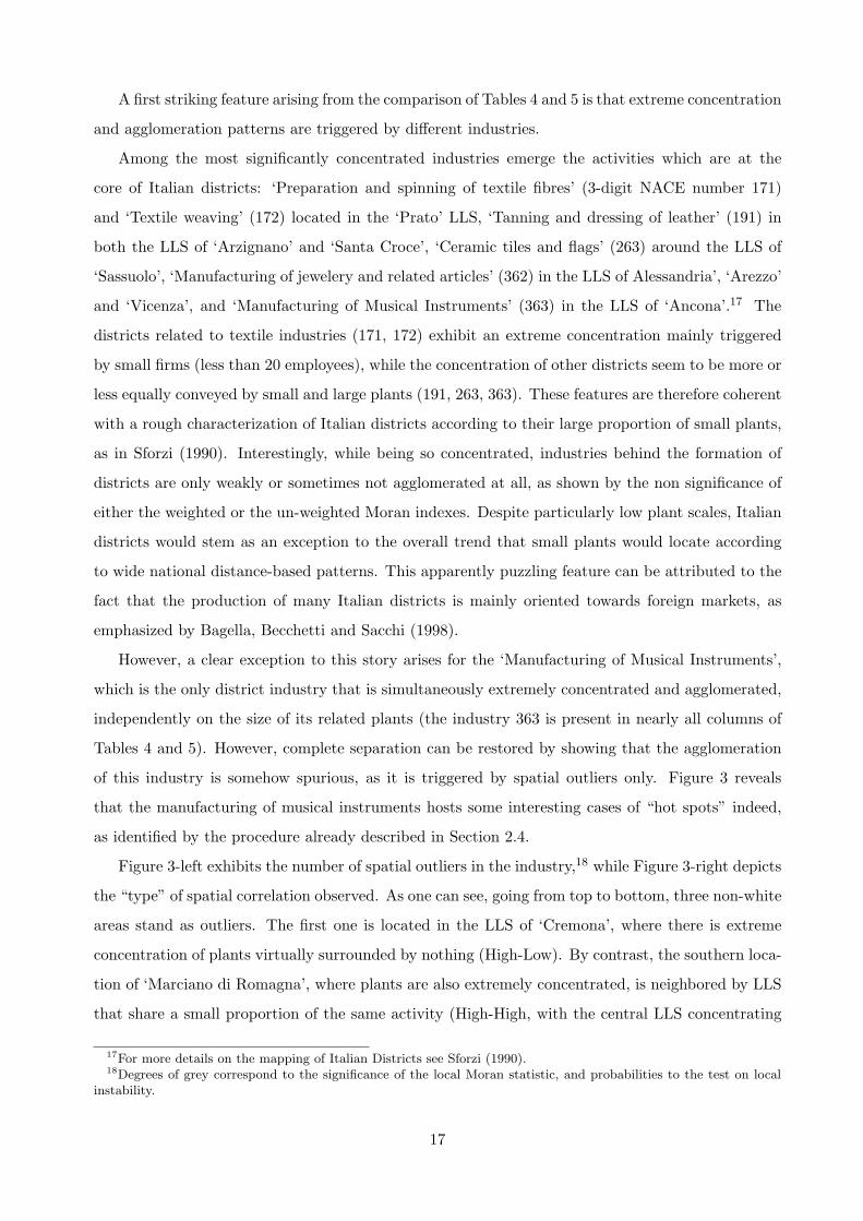
of this industry is somehow spurious, as it is triggered by spatial outliers only. Figure 3 reveals

that the manufacturing of musical instruments hosts some interesting cases of “hot spots” indeed,

as identified by the procedure already described in Section 2.4.

Figure 3-left exhibits the number of spatial outliers in the industry,18 while Figure 3-right depicts

the “type” of spatial correlation observed. As one can see, going from top to bottom, three non-white

areas stand as outliers. The first one is located in the LLS of ‘Cremona’, where there is extreme

concentration of plants virtually surrounded by nothing (High-Low). By contrast, the southern loca-

tion of ‘Marciano di Romagna’, where plants are also extremely concentrated, is neighbored by LLS

that share a small proportion of the same activity (High-High, with the central LLS concentrating

17For more details on the mapping of Italian Districts see Sforzi (1990).18Degrees of grey correspond to the significance of the local Moran statistic, and probabilities to the test on local

instability.

17

Figure 3: Spatial Outliers in the ‘Manufacturing of Musical Instruments’ Industry

most of the activity). Finally, the third eastern-southern area is the well-known district of musical

instruments centered around ‘Castelfidardo’, and which includes the neighboring labor markets of

‘Ancona’, ‘Macerata’, ‘Osimo’, and ‘Recanati’ in which plants are also extremely concentrated (also

High-High, but with both the central and neighboring LLS highly concentrated). When excluding

spatial outliers from this industry (which still leads to 110 LLS left with non-zero employment), we

find that the ‘Manufacturing of Musical Instruments’ industry is actually not significantly agglomer-

ated anymore (i.e the Moran index is not significant). Therefore, the extreme case of agglomeration

revealed by data on this industry is due to the outlier nature of some LLS only (6 over 116), and

does not reflect an overall tendency for the industry of musical instruments to be more agglomerated

on average than others.

In the group of the most concentrated industries within big plants (See Table 5), we find the

‘Manufacturing of other transport equipment’ (355). One can see from Table 15 in Appendix B,

that the Moran index for this industry is negative but not significant. Caution is thus needed in

interpreting the distribution patterns of this industry. Indeed, in 1996, there were only four Italian

plants with at least 20 employees in the transport equipment industry. They were all located in

the northern small triangle of ‘Bergamo’, ‘Modena’, and ‘Imola’ LLS. Notice that this number is

particularly low in comparison with the 784 LLS geographic units, meaning that the Moran is biased,

as recalled in Section 2.4. Mass-production activities such as ‘Publishing’ (221) or ‘Reproduction of

18

recorded media’ (223), are also found to be extremely concentrated in the category of large plants,

but not agglomerated, as testified by the significant negative values of the related weighted Moran.

These results suggest that extreme concentration patterns occurring within the boundaries of

local labor markets, such as the previous, translate into dense clusters of economic activities and

therefore may generate productivity gains for the related industries/plants and locations. Such

gains could stem from either strong increasing returns to scale (as testified by their extremely low

number of large plants) or localized spillovers created through density. Possibly coupled with low

international transport costs, they may enable plants to target foreign markets on top of domestic

ones.

Among the activities exhibiting the strongest positive spatial auto-correlation within the sample

of small plants, the food industries are over-represented (152, 153, 154, and 158). Moreover, as

apparent from Table 14 in Appendix B, the number of spatial outliers is particularly large for these

industries, meaning that related co-location patterns are triggered by numerous extreme cases of

agglomeration. Other activities related to the final stage of production such as ‘Manufacturing of

footwear’ (193) exhibit the same pattern. In the sample of activities displaying the strongest spatial

dependence within the counterpart sample of large plants, one can find upstream industries such

as ‘Manufacturing of other wearing apparel and accessories’ (182), ‘Manufacturing of other special

purpose machinery’ (295), or ‘Manufacturing of refined petroleum products’ (232).

In both previous cases, agglomeration patterns are likely to prevail because firms want to save on

transport costs (due to either perishability, voluminosity, specific transport modes or customers’ face-

to-face requirements), and therefore locate in the close proximity of the potentially largest number

of buyers (consumers or downstream industries). High transport costs and demand linkages (final

and intermediate) could be at the core of such wide distance-based location patterns.

The comparison of concentration and agglomeration patterns across different industries is there-

fore insightful in several ways. The results that plants located in the areas where an industry

concentrates are larger, on average, than outside such areas, is important as regards efficiency. The

productivity gains that could arise from extremely dense areas may enable large firms to serve

markets located far beyond the boundaries of neighboring markets. This would translate into (i)

a geographic distribution that would not be sensitive to domestic distances, (ii) a production of

goods, on average, less domestically customized or more oriented towards distant markets. Indus-

tries hosting the largest plants should therefore testify of a larger proportion of either inter-regional

or international shipments than of inter-labor market exchanges. By contrast, small establishments,

which exhibit the converse tendency of being more sensitive to inter-LLS distances, would need to

save on transport costs by locating close to domestic demand, the key determinant of the agglom-

19

eration in this case. Most salient exceptions to this overall trend are the Italian districts formed

around small concentrated plants. The feature that such districts do not show any distance-based

co-location patterns at the scale of LLS is fully compatible with an underlying criterion defining

districts on the basis on exports oriented mainly towards foreign (and not domestic) markets.

5 Robustness checks and long-run trends

This section addresses the robustness of the positive (negative) correlation found between concentra-

tion (agglomeration) and plant size (Section 5.1). Furthermore it also explores the time-dimension of

our panel data, by investigating the evolution of concentration and agglomeration patterns over the

period 1981-1996, and by focusing on how changes have been triggered by large rather than small

plants, beyond the consideration of specific industry characteristics (Section 5.2).

5.1 Robustness checks

We first investigate the robustness of the results presented in Section 4 to changes in the geographic,

industrial, and plant partitions.

Controlling for the MAUP and the distance bias: The case of Italian ‘provincie’

Are the trends provided in Section 4 dependent upon the geographic partition of Italian space

into Local Labor Systems? In other words, is the positive (negative) correlation found between

concentration (agglomeration) and plant size robust to the MAUP? To address this question, we

present a brief analysis of the concentration and agglomeration patterns obtained for the 95 Italian

NUTS3 regions. As apparent from the comparison of Table 6 and its LLS counterpart (Table 3

presented in Section 4), both the average concentration and agglomeration indexes increase with the

geographical scale of study.

Table 6: Concentration and agglomeration indexes (95 ‘provincie’): Small vs large plants

Sample of small plants Sample of large plantsConcentration Agglomeration Concentration AgglomerationγEG γUW IW IUW γEG γUW IW IUW

Average value 0.034 0.030 0.024 0.033 0.049 0.046 0.007 0.013Average st. deviation 0.0025 0.0015 0.0126 0.0133 0.0069 0.0030 0.0124 0.0125R2 0.89 0.81 0.82 0.65R2 ranks 0.92 0.70 0.75 0.58Number of manuf. plants 549,747 549,747 41,363 41,363

The result that concentration rises when considering wider spatial units is now well established.19

19See among others Kim (1995), Ellison and Glaeser (1997), Maurel and Sedillot (1999), Pagnini (2003) and Barrios,

20

This feature suggests that concentration processes are likely to depend upon other spillovers than

those driven, for instance, by labor market pooling. Spatial auto-correlation also seems to occur

at a larger scale than LLS. Nevertheless, as differences between the Moran indexes calculated for

LLS and provinces are rarely significant, we cannot draw any general conclusion from this result.

However, the overall trend found for the relation between concentration, agglomeration, and plant

size is similar to that found for LLS. At the scale of Italian administrative NUTS3 regions, large

plants still exhibit a clear tendency to concentrate more in the regions where other large plants

are already located than elsewhere. As regards agglomeration, small plants display more spatial

auto-correlated patterns than large plants.

Furthermore, as shown in Table 7, the consideration of real road distances between regions instead

of bilateral great-circle distances, does not lead to drastic changes in the results.

Table 7: Moran indexes computed with real road distances (95 ‘provincie’)

Sample of small plants Sample of big plantsIW IUW IW IUW

Average value 0.032 0.040 0.011 0.016Average st. deviation 0.0141 0.0148 0.0140 0.0141R2 0.79 0.75R2 ranks 0.78 0.70Number of manuf. plants 549,747 41,363

Discrepancies between employment- and plant-based Moran indexes decrease slightly for the

sample of large plants (correlations in both level and ranks increase). Although the mean Moran is

now larger for both types of plants, agglomeration indexes are still around 3 times larger for small

plants than for large establishments. The similarity of the results based on both the effective and

linear distances is not surprising, yet. As shown by Combes and Lafourcade (2005) for France, linear

distance is indeed a very good substitute to effective distance in the case of cross-section analysis.

However, as the distance bias worsens when passing from cross-section to time-series analysis, we

will have to be cautious in interpreting the long-run trends provided in Section 5.2.

Comparison between 2-digit and 3-digit industries

In order to test whether the results are sensitive to how manufacturing products are defined,

we also perform the calculation of indexes using the 2-digit classification of industries. Although

the qualitative relation found between concentration, agglomeration and the size of plants is not

affected, changes occur in the level of indexes, once again. Focusing on the geographic scale of LLS,

we find that the un-weighted index of concentration (agglomeration) decreases (increases) by 58%

Bertinelli, Strobl and Teixeira (forthcoming).

21

(36%), when computed on this broadly defined category of manufacturing industries. The feature

that concentration decreases with the level of industry aggregation suggests that spillovers in the

manufacturing industry are less likely to operate between the 3-digit industries than within each

industry. Furthermore, this result does not depend upon the definition of regions we choose.20 This

feature is not surprising and was already emphasized by Ellison and Glaeser (1997), and Maurel and

Sedillot (1999), as regards the concentration perspective. Our analysis complements their findings in

assessing that the distribution of plants within the broad 2-digit category is by contrast characterized

by a stronger distance-based pattern (more agglomeration). However, the variances of the 2-digit

indexes are so large with respect to the corresponding 3-digit sub-industries that the differences are

rarely significant.

Sensitivity to the dichotomic partition of plants and to the plant threshold chosen

The fact that a positive (although strongly reduced) gap between employment- and plant-based

indexes still remains after correcting for the heterogeneity of plant size (See Table 3) indicates that

more complex partition schemes than the small-large dichotomic one would probably be preferable.

We present now the results of splitting the universe of Italian plants into three categories instead

of two: small (less than 15 employees), medium (between 15 and 100 employees) and large (more

than 100 employees) plants. This partition has the advantages of both considering the cut-off of

15 employees which, as recalled in Section 3.2, may be more relevant for Italy, and of dividing the

sample into 3 rather balanced employment groups instead of two.

Table 8: Concentration and agglomeration for 3 sub-samples of plants (784 LLS)

Concentration (γUW ) Agglomeration (IUW )Small Medium Large Small Medium Large

Average value 0.022 0.032 0.053 0.019 0.013 0.005Average st. deviation 0.0016 0.0020 0.0200 0.0032 0.0027 0.0024Number of manuf. plants 534,427 51,298 5,385 534,427 51,298 5,385Number of manuf. workers 1,783,799 1,600,103 1,471,875 1,783,799 1,600,103 1,471,875

As apparent from Table 8, which is the counterpart of the Table 3 presented in Section 4, a further

exploitation of the plants employment distribution leads to virtually the same results: We find that

large plants are more concentrated than medium establishments, that, in return concentrate more

than small plants. And the converse tendency prevails for agglomeration. The correlation story

between concentration, agglomeration and plant size thus remains unchanged to that of Section 4.

The results presented in this sub-section suggest however that it could be better to model it in a

continuous framework: The larger (lower) the employment scale of plants, the larger the tendency

to concentrate (agglomerate).

20Results on 2-digit industries (for both LLS and NUTS3 regions) are available upon request.

22

5.2 Time evolution of concentration and agglomeration patterns

In order to further assess the positive (negative) relationship found between concentration (agglom-

eration) and plant size, we present in Table 9 the result of the following industry fixed-effects panel

regression: For the three census years 1981, 1991 and 1996, we use the concentration and agglomer-

ation indexes as independent variables to be regressed on size=ln(average size of establishments) in

each industry, with us being the industry fixed-effect.

Table 9: Panel regression of indexes on Size=ln(average size of plants) (784 LLS)

Coefficients or Tests ValuesConcentration (γUW ) Agglomeration (IUW )

Size 0.0248* (0.0039) -0.0055* (0.0012)Constant -0.0437* (0.0106) 0.0327* (0.0033)

R2 0.17 0.14Number of observations 309 309Number of years 3 3Industry dummies Yes YesTime dummies Yes Yes

Note: Standard errors in brackets. * denotes significance at the 1%level.

As apparent from Table 9, the impact of size on concentration (agglomeration) is positive (nega-

tive) and significant at 1%, as expected. These results suggest that plant scale has an impact on the

spatial distribution of establishments which is not simply driven by (time-invariant) sector specific

characteristics such as factor endowments or raw materials.

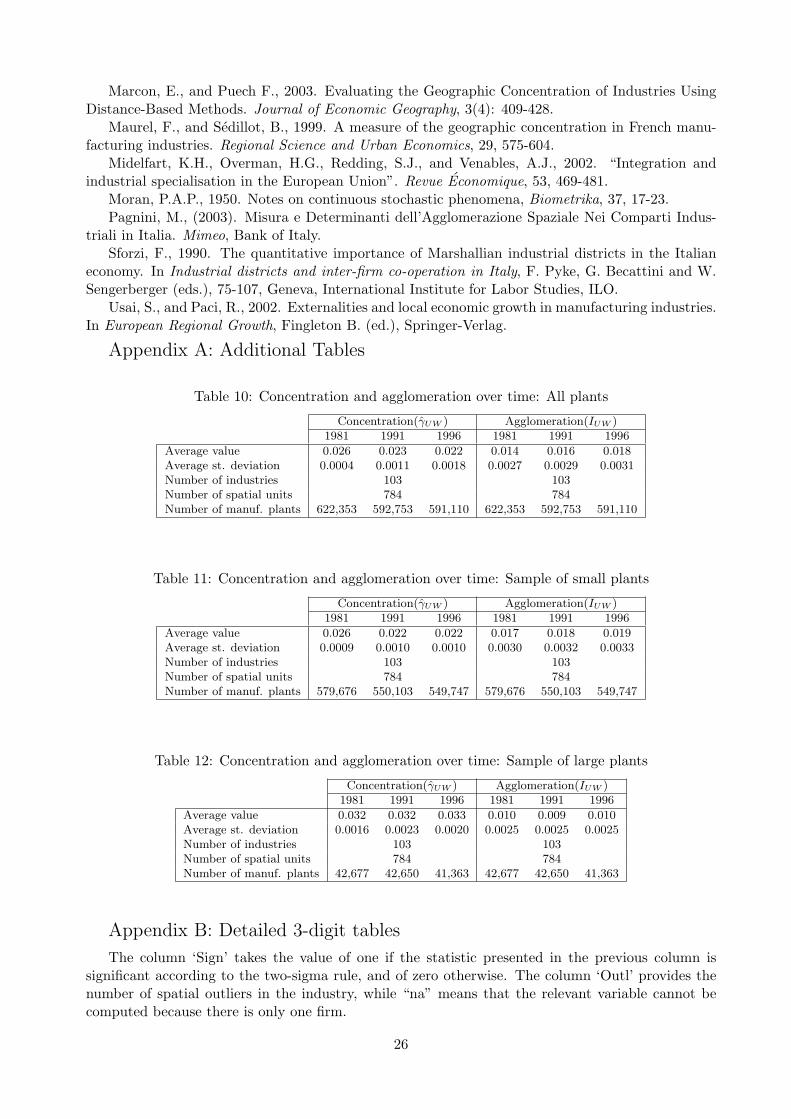
As for the time evolution of concentration and agglomeration patterns, Table 10 in Appendix

A reveals that mean concentration has slightly decreased while mean agglomeration has increased

over the period 1981-1996. Kim (1995) finds a similar declining pattern of concentration after

the second world war for the U.S. More recent studies for Europe, such as Brulhart (2001) or

Midelfart, Overman, Redding and Venables (2002) lead to more controversial results, with some

industries experiencing an increase and some others a decrease of concentration.21 Interestingly, by

disentangling the time evolution according to the size of plants (See Tables 11 and 12 in Appendix

A), one can see that the dynamics is mainly conveyed by small plants, with big units showing a

relatively stabler pattern.

6 Conclusions

This paper analyzes the spatial distribution of manufacturing activities in Italy by focusing on two

different features. The first feature, concentration, can be defined as the degree of variability across

21Both studies relate the changes in concentration to industry characteristics such as increasing return to scales,skills or R&D intensity.

23

data for a given partition of space. The second feature, agglomeration, explicitly considers distances

among observations and thus their spatial dependence. Although there exists many studies focusing

on concentration, agglomeration has received relatively less attention by the profession.

Investigating the influence of plant size on both the concentration and agglomeration distribution

patterns is instructive in several ways. Whereas the result that large plants tend to be more con-

centrated than small units comforts some evidence already pointed by other few studies, the feature

that small plants are more agglomerated than large ones is innovative. While large plants would ex-

hibit a clear tendency to cluster within narrow geographical units such as local labor systems, small

establishments, by contrast would thus rather co-locate within wider areas in which a distance-based

pattern emerges. These features are robust to changes in the partition of space, industries, plants,

and in the distance measurement. Controlling for time-invariant sector specific characteristics, such

as raw material or natural resources, does not alter the picture either. Such results highlight some of

the underlying economic mechanisms driving plant location choices. Differences in transport costs

intensity between small and large plants is a plausible explanation of the different distribution pat-

terns obtained. The need for small firms to save on transport costs by locating close to domestic

demand, would be a key determinant of the strong distance-based patterns found for the industries

hosting small plants, such as food processing. By contrast, industries hosting large plants or Ital-

ian districts would testify of a higher proportion of either inter-regional or international activities.

Moreover, a closer look at the time evolution of the geographic distribution of Italian firms reveals

declining (increasing) concentration (agglomeration) patterns, the dynamics being mainly conveyed

by small plants.

Further lines of research would deserve attention for future work. A first valuable contribution

would be to measure both the narrow and large scope spillovers within the same integrated theoretical

framework, instead of combining two types of indexes. This would enrich the analysis by opening

the way to identifying different types of externalities. Another interesting topic is related to the

causality of the relationship found between plant size, concentration and agglomeration. As circular

causation may be at work, structural econometrics would call for clarifying theoretical contributions.

References

Anselin, L., 1988. Spatial Econometrics: Methods and Models. Kluwer Academic Publishers.Anselin, L., 1995. Local Indicators of Spatial Association-LISA. Geographical Analysis, 27(2),

93-115.Arbia, G., 1989. Spatial Data Configuration in Statistical Analysis of Regional Economic and

Related Problems. Kluwer, Dordrecht.Arbia, G., 2001a. Modelling the geography of economic activities on a continuous space. Papers

in Regional Science, 80, 411-424.

24

Arbia, G., 2001b. The role of spatial effects in the empirical analysis of regional concentration.Journal of Geographical Systems, 3, 271-281.

Bagella, M., L. Becchetti and S. Sacchi, 1998. The positive link between geographical agglomer-ation and export intensity: The engine of Italian endogenous growth?. Economic Notes, Monte deiPaschi di Siena, 27(1), 1-34.

Barrios, S., Bertinelli, L., and Strobl, E., 2003. Geographic Concentration and EstablishmentScale: Can Panel Data tell us more?. CORE Discussion Papers, 36.

Barrios, S., Bertinelli, L., Strobl, E., and Teixeira, A.C., forthcoming. The Dynamics of Agglom-eration: Evidence From Ireland and Portugal. Journal of Urban Economics.

Brulhart M., 2001. “Evolving Geographical Specialisation of European Manufacturing Indus-trie”. Weltwirtschaftliches Archiv, 137(2), 215-243.

Ciccone, A., 2002. Agglomeration effects in Europe. European Economic Review, 46, 213-227.Ciccone, A., and Hall, R.E., 1996. Productivity and the density of economic activities. American

Economic Review, 86(1), 54-70.Cliff, A.D., and Ord, J. K., 1981. Spatial Processes: Models and Applications. Pion, London.Combes, P-P., and Lafourcade, M., 2005. Transport Costs: Measures, determinants and regional

policy implications for France. Journal of Economic Geography, in press.Combes, P.-P., and Overman, H.G., 2004. The Spatial Distribution of Economic Activities in

the European Union. In Handbook of Regional and Urban Economics, Vol.4, J.V. Henderson andJ.-F. Thisse (eds.), Elsevier-North Holland, Amsterdam.

Devereux, M.P., Griffith, R., and Simpson, H., 2004. The geographic distribution of productionactivity in the UK. Regional Science and Urban Economics, 34(5), 533-564.

Disdier, A. C., and Head, K., 2004. The Puzzling Persistence of the Distance Effect on BilateralTrade. Mimeo. http://pacific.commerce.ubc.ca/keith/Papers/meta.pdf.

Duranton, G., and Overman, H.G., 2004. Testing for Localisation Using Micro-Geographic Data.Review of Economic Studies, forthcoming.

Ellison, G., and Glaeser, E., 1997. Geographic concentration in US manufacturing industries: Adartboard approach. Journal of Political Economy, 105, 889-927.

Fujita, M., and Thisse, J.F. (2001) Economics of Agglomeration: Cities, Industrial Location, andRegional Growth, Cambridge University Press, Cambridge, 466p.

Fujita, M., Krugman, P., and Venables, A.J. (1999) The Spatial Economy: Cities, Regions, andInternational Trade, MIT Press, Cambridge, Massachusetts, 367p.

Fujita, M., Henderson, J.V. and Mori, T., 2004. Spatial Distribution of Economic Activities inJapan and China. In Handbook of Regional and Urban Economics, Vol.4, J.V. Henderson and J.-F.Thisse (eds.), Elsevier-North Holland, Amsterdam.

Getis, A., and Ord, J.K., 1992. The analysis of spatial association by use of distance statistics.Geographical Analysis, 24, 189-206.

Harris, C.D., 1954. The Market as a Factor in the Localization of Industry in the United States.Annals of the Association of American Geographers, 44, 315-348.

Holmes, T.J., and Stevens, J.J., 2004. Spatial Distribution of Economic Activities in NorthAmerica. In Handbook of Regional and Urban Economics, Vol.4, J.V. Henderson and J.-F. Thisse(eds.), Elsevier-North Holland, Amsterdam.

Holmes, T.J., and Stevens, J.J., 2002. Geographic concentration and establishment scale. Reviewof Economics and Statistics, 84, 682-690.

Kim, S., 1995. Expansion of Markets and the Geographic Concentration of Economic activities:The Trends in U.S. Regional Manufacturing structure, 1860-1987. Quarterly Journal of Economics,110(4), 881-908.

Lafourcade, M., and Mion, G., 2003. Concentration, Agglomeration and the Size of plants: Dis-entangling the Source of Co-Location Externalities. Core discussion Paper 91, Universite Catholiquede Louvain.

25

Marcon, E., and Puech F., 2003. Evaluating the Geographic Concentration of Industries UsingDistance-Based Methods. Journal of Economic Geography, 3(4): 409-428.

Maurel, F., and Sedillot, B., 1999. A measure of the geographic concentration in French manu-facturing industries. Regional Science and Urban Economics, 29, 575-604.

Midelfart, K.H., Overman, H.G., Redding, S.J., and Venables, A.J., 2002. “Integration andindustrial specialisation in the European Union”. Revue Economique, 53, 469-481.

Moran, P.A.P., 1950. Notes on continuous stochastic phenomena, Biometrika, 37, 17-23.Pagnini, M., (2003). Misura e Determinanti dell’Agglomerazione Spaziale Nei Comparti Indus-

triali in Italia. Mimeo, Bank of Italy.Sforzi, F., 1990. The quantitative importance of Marshallian industrial districts in the Italian

economy. In Industrial districts and inter-firm co-operation in Italy, F. Pyke, G. Becattini and W.Sengerberger (eds.), 75-107, Geneva, International Institute for Labor Studies, ILO.

Usai, S., and Paci, R., 2002. Externalities and local economic growth in manufacturing industries.In European Regional Growth, Fingleton B. (ed.), Springer-Verlag.

Appendix A: Additional Tables

Table 10: Concentration and agglomeration over time: All plants

Concentration(γUW ) Agglomeration(IUW )1981 1991 1996 1981 1991 1996

Average value 0.026 0.023 0.022 0.014 0.016 0.018Average st. deviation 0.0004 0.0011 0.0018 0.0027 0.0029 0.0031Number of industries 103 103Number of spatial units 784 784Number of manuf. plants 622,353 592,753 591,110 622,353 592,753 591,110

Table 11: Concentration and agglomeration over time: Sample of small plants

Concentration(γUW ) Agglomeration(IUW )1981 1991 1996 1981 1991 1996

Average value 0.026 0.022 0.022 0.017 0.018 0.019Average st. deviation 0.0009 0.0010 0.0010 0.0030 0.0032 0.0033Number of industries 103 103Number of spatial units 784 784Number of manuf. plants 579,676 550,103 549,747 579,676 550,103 549,747

Table 12: Concentration and agglomeration over time: Sample of large plants

Concentration(γUW ) Agglomeration(IUW )1981 1991 1996 1981 1991 1996

Average value 0.032 0.032 0.033 0.010 0.009 0.010Average st. deviation 0.0016 0.0023 0.0020 0.0025 0.0025 0.0025Number of industries 103 103Number of spatial units 784 784Number of manuf. plants 42,677 42,650 41,363 42,677 42,650 41,363

Appendix B: Detailed 3-digit tables

The column ‘Sign’ takes the value of one if the statistic presented in the previous column issignificant according to the two-sigma rule, and of zero otherwise. The column ‘Outl’ provides thenumber of spatial outliers in the industry, while “na” means that the relevant variable cannot becomputed because there is only one firm.

26

Table 13: LLS - 3-digit - All plants

NACE Industry γUW σ(γUW ) Sign γEG σ(γEG) Sign IUW σ(IUW ) Sign IW σ(IW ) Sign Outl.

151 prod. proc. pres. of meat 0.0109 0.0000 1 0.0085 0.0005 1 0.0146 0.0025 1 0.0143 0.0026 1 14152 proc. and pres. of fish 0.0218 0.0003 1 0.0200 0.0033 1 0.0389 0.0048 1 0.0124 0.0024 1 17153 proc. and pres. of fruit 0.0137 0.0001 1 0.0194 0.0006 1 0.0865 0.0106 1 0.0431 0.0053 1 15154 man. of veg. and anim oils 0.0158 0.0000 1 0.0157 0.0002 1 0.1067 0.0130 1 0.0637 0.0078 1 19155 man. of dairy prod 0.0071 0.0000 1 0.0036 0.0004 1 0.0352 0.0044 1 0.0181 0.0027 1 17156 man. of grain mill prod 0.0084 0.0001 1 0.0079 0.0006 1 0.0354 0.0044 1 0.0111 0.0026 1 12157 man. of prep anim feeds 0.0093 0.0002 1 0.0101 0.0012 1 0.0196 0.0025 1 0.0093 0.0026 1 13158 man. of other food prod 0.0043 0.0000 1 0.0019 0.0001 1 0.0673 0.0083 1 0.0324 0.0041 1 14159 man. of beverages 0.0091 0.0000 1 0.0033 0.0003 1 0.0391 0.0049 1 0.0232 0.0030 1 12160 man. of tobacco prod 0.0324 0.0009 1 0.0081 0.0050 0 0.0357 0.0045 1 0.0215 0.0027 1 18171 prep. and spin of text fibres 0.2151 0.0000 1 0.0624 0.0003 1 0.0014 0.0012 1 0.0130 0.0023 1 5172 textile weaving 0.2170 0.0000 1 0.0505 0.0004 1 0.0010 0.0011 1 0.0092 0.0024 1 4173 finishing of textiles 0.0676 0.0001 1 0.0745 0.0003 1 0.0030 0.0020 1 0.0045 0.0022 1 11174 man. of made-up text art 0.0057 0.0000 1 0.0101 0.0002 1 0.0030 0.0026 0 0.0075 0.0026 1 7175 man. of other textiles 0.0142 0.0000 1 0.0125 0.0003 1 0.0068 0.0024 1 0.0153 0.0025 1 6176 man. of knitt and croch fab 0.0227 0.0000 1 0.0192 0.0002 1 0.0187 0.0024 1 0.0112 0.0025 1 16177 man. of knitt and croch art 0.0132 0.0000 1 0.0144 0.0001 1 0.0232 0.0029 1 0.0180 0.0026 1 26181 man. of leather clothes 0.0362 0.0001 1 0.0443 0.0003 1 0.0192 0.0025 1 0.0164 0.0021 1 11182 man. of other wear apparel 0.0042 0.0000 1 0.0052 0.0000 1 0.0255 0.0032 1 0.0210 0.0027 1 17183 dress and dyeing of fur 0.0094 0.0001 1 0.0097 0.0003 1 -0.0001 0.0025 0 0.0025 0.0024 0 3191 tan and dres of leather 0.2061 0.0001 1 0.2082 0.0002 1 -0.0012 0.0021 0 -0.0001 0.0022 0 6192 man. of luggage, bags 0.0688 0.0000 1 0.0809 0.0001 1 0.0019 0.0011 1 0.0019 0.0011 1 16193 man. of footwear 0.0288 0.0000 1 0.0274 0.0001 1 0.0551 0.0068 1 0.0437 0.0054 1 9201 sawmil and impregn of wood 0.0083 0.0000 1 0.0115 0.0002 1 0.0225 0.0029 1 0.0218 0.0028 1 16202 man. of venter sheets, plywood 0.0205 0.0003 1 0.0177 0.0014 1 0.0150 0.0026 1 0.0051 0.0026 1 9203 man. of uilders’carp and joinery 0.0052 0.0000 1 0.0051 0.0000 1 0.0425 0.0053 1 0.0243 0.0031 1 13204 man. of wooden containers 0.0056 0.0001 1 0.0067 0.0003 1 0.0311 0.0039 1 0.0150 0.0026 1 19205 man. of other prod. of wood 0.0057 0.0000 1 0.0070 0.0001 1 0.0196 0.0025 1 0.0160 0.0026 1 17211 man. of pulp, paper 0.0105 0.0004 1 0.0052 0.0022 1 0.0170 0.0025 1 0.0030 0.0027 0 6212 man. of art of paper 0.0030 0.0000 1 0.0037 0.0002 1 0.0065 0.0024 1 0.0009 0.0025 0 15221 publishing 0.0419 0.0000 1 0.0851 0.0006 1 -0.0032 0.0020 0 -0.0048 0.0017 1 3222 printing and rel services 0.0061 0.0000 1 0.0115 0.0001 1 0.0058 0.0022 1 -0.0016 0.0021 0 3223 reproduction of rec media 0.0325 0.0004 1 0.2605 0.0034 1 -0.0044 0.0017 0 -0.0028 0.0006 1 2231 man. of coke oven prod 0.0111 0.0451 0 0.0941 0.1687 0 -0.0021 0.0024 0 -0.0016 0.0006 0 5232 man. of refined petrol prod 0.0048 0.0002 1 0.0343 0.0035 1 0.0693 0.0085 1 0.0074 0.0023 1 27233 processing of nuclear fuel 0.0341 0.1129 0 0.4620 0.8028 0 -0.0024 0.0020 0 -0.0021 0.0005 0 4241 man. of basic chemicals 0.0045 0.0001 1 0.0100 0.0013 1 0.0065 0.0021 1 0.0016 0.0026 0 28242 man. of agro-chem prod 0.0099 0.0014 1 0.0293 0.0058 1 0.0042 0.0026 1 0.0039 0.0024 1 17243 man. of paints, varnish 0.0022 0.0001 1 0.0212 0.0008 1 0.0073 0.0025 1 0.0003 0.0016 0 34244 man. of pharmac, med chem 0.0670 0.0002 1 0.1210 0.0012 1 -0.0017 0.0017 0 -0.0022 0.0013 0 1245 man. of soap and deterg 0.0074 0.0001 1 0.0259 0.0014 1 0.0036 0.0020 1 0.0056 0.0022 1 20246 man. of other chem prod 0.0078 0.0001 1 0.0174 0.0011 1 0.0070 0.0018 1 0.0051 0.0022 1 21247 man. of man-made fibres 0.0181 0.0021 1 0.0058 0.0070 0 0.0213 0.0027 1 0.0008 0.0026 0 11251 man. of rubber prod 0.0105 0.0001 1 0.0089 0.0015 1 0.0138 0.0021 1 0.0139 0.0025 1 10252 man. of plastic prod 0.0016 0.0000 1 0.0022 0.0001 1 0.0284 0.0036 1 0.0259 0.0033 1 11261 man. of glass 0.0105 0.0000 1 0.0104 0.0009 1 0.0143 0.0021 1 0.0022 0.0025 0 12262 man. of refr and non-refr ceramics 0.0161 0.0000 1 0.0225 0.0006 1 0.0228 0.0029 1 0.0088 0.0023 1 18263 man. of ceramic tiles and flags 0.1404 0.0002 1 0.2192 0.0009 1 0.0124 0.0016 1 0.0113 0.0015 1 6264 man. of bricks, tiles 0.0134 0.0002 1 0.0123 0.0007 1 0.0280 0.0035 1 0.0135 0.0026 1 16265 man. of cement, lime 0.0126 0.0003 1 0.0081 0.0021 1 0.0469 0.0058 1 0.0056 0.0026 1 22266 man. of art. of concr 0.0062 0.0000 1 0.0062 0.0001 1 0.0533 0.0066 1 0.0230 0.0029 1 11267 cutting, finish of stone 0.0105 0.0000 1 0.0172 0.0001 1 0.0341 0.0043 1 0.0223 0.0028 1 17268 man. of other non-met min prod 0.0024 0.0002 1 0.0070 0.0007 1 0.0131 0.0027 1 0.0023 0.0026 0 18271 man. of basic iron, steel 0.0115 0.0008 1 0.0520 0.0074 1 0.0179 0.0026 1 0.0001 0.0021 0 8272 man. of tubes 0.0034 0.0004 1 0.0064 0.0044 0 0.0129 0.0026 1 0.0046 0.0020 1 19273 other 1st proc of iron, steel 0.0086 0.0001 1 0.0118 0.0011 1 0.0119 0.0020 1 0.0055 0.0023 1 24274 man. of non-ferr met 0.0083 0.0003 1 0.0156 0.0022 1 0.0140 0.0025 1 0.0028 0.0024 0 19275 casting of metals 0.0069 0.0001 1 0.0073 0.0007 1 0.0325 0.0041 1 0.0146 0.0026 1 8281 man. of struct and met prod 0.0028 0.0000 1 0.0022 0.0000 1 0.0472 0.0058 1 0.0207 0.0027 1 14282 man. of tanks, reserv 0.0031 0.0001 1 0.0064 0.0013 1 0.0114 0.0027 1 0.0061 0.0027 1 29283 man. of steam gen 0.0258 0.0020 1 0.0108 0.0305 0 0.0037 0.0024 1 -0.0031 0.0018 0 15284 forg, press, stamp 0.0083 0.0001 1 0.0106 0.0002 1 0.0224 0.0029 1 0.0312 0.0039 1 9285 treat, coat of met 0.0028 0.0000 1 0.0030 0.0000 1 0.0457 0.0057 1 0.0319 0.0040 1 20286 man. of cutlery, tools 0.0074 0.0000 1 0.0073 0.0003 1 0.0240 0.0030 1 0.0302 0.0038 1 12287 man. of other fab metal prod 0.0019 0.0000 1 0.0040 0.0000 1 0.0324 0.0041 1 0.0159 0.0023 1 29291 man. of machin. for mech power 0.0082 0.0000 1 0.0067 0.0007 1 0.0159 0.0022 1 0.0120 0.0026 1 8292 man. of other gen purpose machin. 0.0009 0.0000 1 0.0024 0.0001 1 0.0066 0.0025 1 0.0150 0.0025 1 24293 man. of agric forestry machin. 0.0088 0.0000 1 0.0141 0.0009 1 0.0184 0.0024 1 0.0154 0.0026 1 9294 man. of machine tools 0.0045 0.0001 1 0.0069 0.0006 1 0.0361 0.0045 1 0.0168 0.0025 1 18295 man. of other spec purp machin. 0.0034 0.0000 1 0.0046 0.0002 1 0.0276 0.0035 1 0.0174 0.0026 1 14296 man. of weapons and ammunition 0.1755 0.0008 1 0.0943 0.0137 1 0.0017 0.0013 1 0.0004 0.0022 0 3297 man. of domestic appliances 0.0045 0.0001 1 0.0183 0.0022 1 0.0171 0.0027 1 0.0041 0.0025 1 25300 man. of off, comp machin. 0.0147 0.0003 1 0.0436 0.0071 1 -0.0016 0.0024 0 -0.0012 0.0018 0 5311 man. of elec. motors, gener 0.0025 0.0001 1 0.0057 0.0006 1 0.0055 0.0025 1 0.0079 0.0026 1 20312 man. of elec. distrib 0.0056 0.0001 1 0.0128 0.0008 1 0.0149 0.0020 1 0.0065 0.0024 1 9313 man. of insulated wire and cable 0.0059 0.0003 1 0.0105 0.0025 1 0.0179 0.0027 1 0.0014 0.0024 0 25314 man. of accum, primar cell 0.0075 0.0008 1 0.0256 0.0083 1 0.0211 0.0027 1 0.0033 0.0024 0 9315 man. of light equip, elect lamps 0.0085 0.0001 1 0.0112 0.0009 1 0.0024 0.0025 0 0.0064 0.0025 1 8316 man. of electrical equip 0.0031 0.0000 1 0.0094 0.0010 1 0.0127 0.0023 1 0.0047 0.0019 1 15321 man. of elec. valves, tubes 0.0070 0.0001 1 0.0124 0.0037 1 0.0124 0.0025 1 -0.0001 0.0023 0 12322 man. of TV, radio for TV 0.0042 0.0000 1 0.0347 0.0014 1 0.0248 0.0031 1 -0.0004 0.0021 0 28323 man. of TV, radio, sound, video 0.0059 0.0003 1 0.0075 0.0035 1 0.0049 0.0025 1 -0.0019 0.0026 0 19331 man. of medic surg equip 0.0038 0.0000 1 0.0078 0.0001 1 0.0124 0.0021 1 -0.0023 0.0024 0 21332 man. of instr. for measur 0.0153 0.0001 1 0.0286 0.0012 1 0.0031 0.0017 1 0.0003 0.0021 0 20333 man. of ind proc control equip 0.0142 0.0002 1 0.0279 0.0026 1 0.0067 0.0018 1 -0.0002 0.0021 0 13334 man. of opt instr, photo equip 0.0272 0.0000 1 0.0542 0.0013 1 0.0260 0.0033 1 0.0338 0.0042 1 8335 man. of watches and clocks 0.0260 0.0011 1 0.0090 0.0068 0 0.0044 0.0020 1 -0.0022 0.0023 0 12341 man. of motor vehicles 0.0266 0.0022 1 0.1411 0.0083 1 0.0041 0.0022 1 -0.0006 0.0013 0 17342 man. of bodies for mot vehic 0.0053 0.0002 1 0.0088 0.0016 1 0.0119 0.0026 1 0.0071 0.0026 1 14343 man. of parts, access for mot vehic 0.0185 0.0001 1 0.0211 0.0007 1 0.0154 0.0020 1 0.0157 0.0021 1 9351 build and repair of boats 0.0195 0.0001 1 0.0336 0.0019 1 0.0230 0.0029 1 0.0110 0.0026 1 20352 man. of rail and tram loco 0.0082 0.0012 1 0.0090 0.0042 1 0.0070 0.0026 1 0.0039 0.0026 1 22353 man. of air and spacecraft 0.0292 0.0012 1 0.0878 0.0062 1 0.0063 0.0024 1 0.0031 0.0021 1 35354 man. of motor and bicycles 0.0159 0.0001 1 0.0285 0.0046 1 0.0083 0.0024 1 0.0000 0.0017 0 10355 man. of other transp equip 0.0000 0.0028 0 0.0091 0.0207 0 -0.0024 0.0027 0 -0.0027 0.0016 0 28361 man. of furniture 0.0117 0.0000 1 0.0161 0.0000 1 -0.0026 0.0023 0 0.0068 0.0025 1 3362 man. of jewellery 0.0361 0.0000 1 0.0859 0.0001 1 0.0017 0.0023 0 0.0004 0.0023 0 9363 man. of musical instruments 0.0505 0.0003 1 0.0816 0.0024 1 0.0094 0.0022 1 0.0305 0.0038 1 3364 man. of sports goods 0.0034 0.0003 1 0.0097 0.0023 1 0.0060 0.0027 1 0.0038 0.0026 0 19365 man. of games and toys 0.0036 0.0002 1 0.0052 0.0016 1 0.0068 0.0026 1 0.0016 0.0024 0 19366 miscell man. n.e.c. 0.0049 0.0000 1 0.0080 0.0003 1 -0.0025 0.0026 0 0.0025 0.0022 0 11371 recycl of met waste and scrap 0.0045 0.0001 1 0.0051 0.0006 1 0.0290 0.0036 1 0.0151 0.0026 1 27372 recycl of non-met waste and scrap 0.0018 0.0002 1 0.0010 0.0007 0 0.0092 0.0027 1 -0.0007 0.0027 0 33

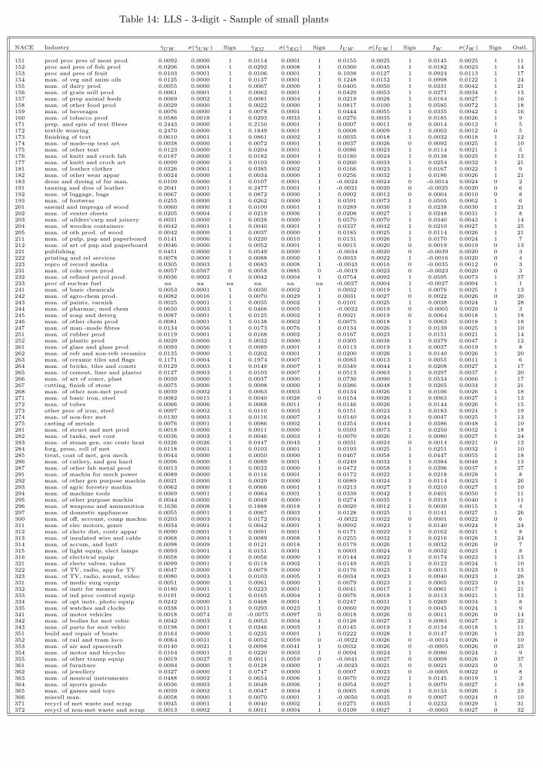
Table 14: LLS - 3-digit - Sample of small plants

NACE Industry γUW σ(γUW ) Sign γEG σ(γEG) Sign IUW σ(IUW ) Sign IW σ(IW ) Sign Outl.

151 prod proc pres of meat prod 0.0092 0.0000 1 0.0114 0.0001 1 0.0155 0.0025 1 0.0145 0.0025 1 11152 proc and pres of fish prod 0.0206 0.0004 1 0.0292 0.0008 1 0.0360 0.0045 1 0.0182 0.0023 1 14153 proc and pres of fruit 0.0103 0.0001 1 0.0106 0.0001 1 0.1038 0.0127 1 0.0924 0.0113 1 17154 man. of veg and anim oils 0.0125 0.0000 1 0.0137 0.0001 1 0.1248 0.0152 1 0.0998 0.0122 1 24155 man. of dairy prod 0.0055 0.0000 1 0.0067 0.0000 1 0.0405 0.0050 1 0.0331 0.0042 1 21156 man. of grain mill prod 0.0061 0.0001 1 0.0062 0.0001 1 0.0429 0.0053 1 0.0271 0.0034 1 13157 man. of prep animal feeds 0.0069 0.0002 1 0.0081 0.0004 1 0.0219 0.0028 1 0.0164 0.0027 1 16158 man. of other food prod 0.0029 0.0000 1 0.0022 0.0000 1 0.0817 0.0100 1 0.0585 0.0072 1 18159 man. of beverages 0.0076 0.0000 1 0.0078 0.0001 1 0.0444 0.0055 1 0.0335 0.0042 1 16160 man. of tobacco prod 0.0586 0.0018 1 0.0293 0.0033 1 0.0276 0.0035 1 0.0185 0.0026 1 9171 prep. and spin of text fibres 0.2443 0.0000 1 0.2150 0.0001 1 0.0007 0.0011 0 0.0014 0.0012 1 5172 textile weaving 0.2470 0.0000 1 0.1849 0.0001 1 0.0008 0.0009 1 0.0003 0.0012 0 5173 finishing of text 0.0610 0.0001 1 0.0861 0.0002 1 0.0035 0.0018 1 0.0032 0.0018 1 12174 man. of made-up text art 0.0038 0.0000 1 0.0072 0.0001 1 0.0037 0.0026 0 0.0092 0.0025 1 10175 man. of other text 0.0123 0.0000 1 0.0204 0.0001 1 0.0086 0.0023 1 0.0114 0.0021 1 5176 man. of knitt and croch fab 0.0187 0.0000 1 0.0182 0.0001 1 0.0180 0.0024 1 0.0138 0.0025 1 13177 man. of knitt and croch art 0.0099 0.0000 1 0.0103 0.0000 1 0.0260 0.0033 1 0.0254 0.0032 1 21181 man. of leather clothes 0.0326 0.0001 1 0.0385 0.0002 1 0.0166 0.0023 1 0.0167 0.0022 1 9182 man. of other wear appar 0.0024 0.0000 1 0.0034 0.0000 1 0.0256 0.0032 1 0.0186 0.0026 1 21183 dress and dyeing of fur man. 0.0109 0.0000 1 0.0107 0.0001 1 -0.0024 0.0024 0 -0.0014 0.0024 0 2191 tanning and dres of leather 0.2041 0.0001 1 0.2477 0.0001 1 -0.0021 0.0020 0 -0.0025 0.0020 0 6192 man. of luggage, bags 0.0667 0.0000 1 0.0872 0.0000 1 0.0002 0.0012 0 0.0004 0.0010 0 8193 man. of footwear 0.0255 0.0000 1 0.0262 0.0000 1 0.0591 0.0073 1 0.0505 0.0062 1 6201 sawmil and impregn of wood 0.0060 0.0000 1 0.0100 0.0001 1 0.0289 0.0036 1 0.0238 0.0030 1 21202 man. of venter sheets 0.0205 0.0004 1 0.0219 0.0006 1 0.0208 0.0027 1 0.0248 0.0031 1 8203 man. of uilders’carp and joinery 0.0031 0.0000 1 0.0028 0.0000 1 0.0570 0.0070 1 0.0340 0.0043 1 14204 man. of wooden containers 0.0042 0.0001 1 0.0040 0.0001 1 0.0337 0.0042 1 0.0210 0.0027 1 25205 man. of oth prod. of wood 0.0042 0.0000 1 0.0037 0.0000 1 0.0185 0.0025 1 0.0114 0.0026 1 21211 man. of pulp, pap and paperboard 0.0141 0.0006 1 0.0220 0.0010 1 0.0131 0.0026 1 0.0170 0.0024 1 7212 man. of art of pap and paperboard 0.0046 0.0000 1 0.0052 0.0001 1 0.0015 0.0020 0 0.0019 0.0019 0 13221 publishing 0.0451 0.0000 1 0.0549 0.0000 1 -0.0034 0.0020 0 -0.0039 0.0020 0 3222 printing and rel services 0.0078 0.0000 1 0.0088 0.0000 1 0.0033 0.0022 1 -0.0016 0.0020 0 4223 repro of record media 0.0305 0.0003 1 0.0683 0.0008 1 -0.0043 0.0016 0 -0.0035 0.0012 0 3231 man. of coke oven prod 0.0057 0.0567 0 0.0058 0.0885 0 -0.0019 0.0023 0 -0.0023 0.0020 0 3232 man. of refined petrol prod. 0.0036 0.0002 1 0.0042 0.0004 1 0.0754 0.0092 1 0.0595 0.0073 1 37233 proc of nuclear fuel na na na na na na -0.0027 0.0004 1 -0.0027 0.0004 1 1241 man. of basic chemicals 0.0053 0.0001 1 0.0030 0.0002 1 0.0032 0.0019 1 0.0076 0.0025 1 13242 man. of agro-chem prod. 0.0082 0.0016 1 0.0070 0.0029 1 0.0031 0.0027 0 0.0022 0.0026 0 20243 man. of paints, varnish 0.0025 0.0001 1 0.0035 0.0002 1 0.0101 0.0025 1 0.0038 0.0024 1 28244 man. of pharmac, med chem 0.0650 0.0003 1 0.0466 0.0005 1 -0.0022 0.0019 0 -0.0005 0.0020 0 3245 man. of soap and deterg 0.0087 0.0001 1 0.0125 0.0002 1 0.0021 0.0019 0 0.0064 0.0018 1 18246 man. of other chem prod 0.0081 0.0001 1 0.0138 0.0002 1 0.0075 0.0018 1 0.0063 0.0018 1 18247 man. of man.-made fibres 0.0134 0.0056 1 0.0173 0.0076 1 0.0134 0.0026 1 0.0139 0.0025 1 10251 man. of rubber prod 0.0119 0.0001 1 0.0168 0.0002 1 0.0167 0.0023 1 0.0151 0.0021 1 14252 man. of plastic prod 0.0029 0.0000 1 0.0032 0.0000 1 0.0305 0.0038 1 0.0379 0.0047 1 12261 man. of glass and glass prod 0.0093 0.0000 1 0.0089 0.0001 1 0.0113 0.0019 1 0.0037 0.0019 1 8262 man. of refr and non-refr ceramics 0.0135 0.0000 1 0.0202 0.0001 1 0.0200 0.0026 1 0.0140 0.0026 1 20263 man. of ceramic tiles and flags 0.1171 0.0004 1 0.1974 0.0007 1 0.0083 0.0013 1 0.0055 0.0011 1 6264 man. of bricks, tiles and constr 0.0129 0.0003 1 0.0149 0.0007 1 0.0349 0.0044 1 0.0208 0.0027 1 17265 man. of cement, lime and plaster 0.0127 0.0003 1 0.0103 0.0007 1 0.0513 0.0063 1 0.0297 0.0037 1 20266 man. of art of concr, plast 0.0039 0.0000 1 0.0037 0.0000 1 0.0730 0.0090 1 0.0534 0.0066 1 17267 cutting, finish of stone 0.0075 0.0000 1 0.0098 0.0000 1 0.0386 0.0048 1 0.0265 0.0034 1 21268 man. of other non-met prod 0.0039 0.0002 1 0.0063 0.0003 1 0.0134 0.0026 1 0.0106 0.0026 1 18271 man. of basic iron, steel 0.0082 0.0015 1 0.0040 0.0028 0 0.0154 0.0026 1 0.0063 0.0027 1 13272 man. of tubes 0.0066 0.0006 1 0.0068 0.0011 1 0.0146 0.0026 1 0.0144 0.0026 1 15273 other proc of iron, steel 0.0097 0.0002 1 0.0110 0.0003 1 0.0151 0.0023 1 0.0183 0.0024 1 19274 man. of non-ferr met 0.0130 0.0003 1 0.0116 0.0007 1 0.0140 0.0024 1 0.0047 0.0025 1 13275 casting of metals 0.0076 0.0001 1 0.0086 0.0002 1 0.0354 0.0044 1 0.0386 0.0048 1 10281 man. of struct and met prod 0.0018 0.0000 1 0.0011 0.0000 1 0.0593 0.0073 1 0.0250 0.0032 1 18282 man. of tanks, met cont 0.0036 0.0002 1 0.0046 0.0003 1 0.0070 0.0026 1 0.0080 0.0027 1 24283 man. of steam gen, exc centr heat 0.0326 0.0026 1 0.0447 0.0043 1 0.0031 0.0024 0 0.0014 0.0021 0 12284 forg, press, roll of met 0.0118 0.0001 1 0.0103 0.0001 1 0.0193 0.0025 1 0.0251 0.0032 1 10285 treat, coat of met, gen mech 0.0044 0.0000 1 0.0050 0.0000 1 0.0467 0.0058 1 0.0447 0.0055 1 18286 man. of cutlery, and gen hard 0.0096 0.0000 1 0.0089 0.0001 1 0.0249 0.0032 1 0.0384 0.0048 1 13287 man. of other fab metal prod 0.0013 0.0000 1 0.0022 0.0000 1 0.0472 0.0058 1 0.0296 0.0037 1 27291 man. of machin for mech power 0.0089 0.0000 1 0.0116 0.0001 1 0.0172 0.0022 1 0.0218 0.0028 1 8292 man. of other gen purpose machin 0.0021 0.0000 1 0.0029 0.0000 1 0.0089 0.0024 1 0.0114 0.0023 1 26293 man. of agric forestry machin 0.0062 0.0000 1 0.0066 0.0001 1 0.0213 0.0027 1 0.0210 0.0027 1 10294 man. of machine tools 0.0069 0.0001 1 0.0064 0.0001 1 0.0339 0.0042 1 0.0401 0.0050 1 11295 man. of other purpose machin 0.0044 0.0000 1 0.0049 0.0000 1 0.0274 0.0035 1 0.0318 0.0040 1 11296 man. of weapons and ammunition 0.1636 0.0008 1 0.1888 0.0018 1 0.0020 0.0012 1 0.0030 0.0015 1 4297 man. of domestic appliances 0.0055 0.0001 1 0.0067 0.0003 1 0.0128 0.0025 1 0.0141 0.0027 1 26300 man. of off, account, comp machin 0.0203 0.0003 1 0.0172 0.0004 1 -0.0022 0.0022 0 0.0001 0.0022 0 6311 man. of elec motors, gener 0.0034 0.0001 1 0.0042 0.0001 1 0.0092 0.0023 1 0.0140 0.0024 1 24312 man. of electr dist, contr appar 0.0090 0.0001 1 0.0091 0.0001 1 0.0171 0.0022 1 0.0162 0.0021 1 8313 man. of insulated wire and cable 0.0068 0.0004 1 0.0089 0.0008 1 0.0255 0.0032 1 0.0216 0.0028 1 24314 man. of accum, and batt 0.0098 0.0009 1 0.0121 0.0018 1 0.0179 0.0026 1 0.0032 0.0026 0 7315 man. of light equip, elect lamps 0.0093 0.0001 1 0.0151 0.0001 1 0.0003 0.0024 0 0.0032 0.0023 1 8316 man. of electrical equip 0.0058 0.0000 1 0.0056 0.0000 1 0.0144 0.0022 1 0.0174 0.0023 1 15321 man. of electr valves, tubes 0.0099 0.0001 1 0.0118 0.0002 1 0.0149 0.0025 1 0.0122 0.0024 1 10322 man. of TV, radio, app for TV 0.0047 0.0000 1 0.0079 0.0000 1 0.0176 0.0023 1 0.0015 0.0023 0 15323 man. of TV, radio, sound, video 0.0080 0.0003 1 0.0103 0.0005 1 0.0034 0.0023 1 0.0040 0.0023 1 26331 man. of medic surg equip 0.0051 0.0000 1 0.0061 0.0000 1 0.0079 0.0023 1 0.0005 0.0023 0 14332 man. of instr for measur 0.0180 0.0001 1 0.0223 0.0001 1 0.0041 0.0017 1 0.0061 0.0017 1 21333 man. of ind proc control equip 0.0191 0.0002 1 0.0165 0.0004 1 0.0076 0.0018 1 0.0113 0.0021 1 13334 man. of opt instr, photo equip 0.0242 0.0000 1 0.0468 0.0001 1 0.0247 0.0031 1 0.0269 0.0034 1 8335 man. of watches and clocks 0.0338 0.0011 1 0.0293 0.0023 1 0.0060 0.0020 1 0.0045 0.0024 1 9341 man. of motor vehicles 0.0018 0.0074 0 -0.0075 0.0097 0 0.0018 0.0026 0 0.0011 0.0026 0 14342 man. of bodies for mot vehic 0.0042 0.0003 1 0.0053 0.0004 1 0.0128 0.0027 1 0.0083 0.0027 1 22343 man. of parts for mot vehic 0.0198 0.0001 1 0.0246 0.0003 1 0.0145 0.0019 1 0.0134 0.0018 1 11351 build and repair of boats 0.0164 0.0000 1 0.0235 0.0001 1 0.0222 0.0028 1 0.0147 0.0026 1 23352 man. of rail and tram loco 0.0064 0.0031 1 0.0052 0.0059 0 -0.0022 0.0026 0 -0.0014 0.0026 0 10353 man. of air and spacecraft 0.0140 0.0021 1 0.0098 0.0041 1 0.0032 0.0026 0 -0.0005 0.0026 0 25354 man. of motor and bicycles 0.0164 0.0001 1 0.0220 0.0003 1 0.0094 0.0024 1 0.0080 0.0024 1 9355 man. of other transp equip 0.0019 0.0027 0 0.0011 0.0059 0 -0.0041 0.0027 0 0.0009 0.0026 0 37361 man. of furniture 0.0094 0.0000 1 0.0128 0.0000 1 -0.0023 0.0021 0 0.0021 0.0023 0 5362 man. of jewellery 0.0327 0.0000 1 0.0747 0.0000 1 0.0007 0.0023 0 -0.0005 0.0022 0 8363 man. of musical instruments 0.0488 0.0002 1 0.0654 0.0006 1 0.0070 0.0022 1 0.0145 0.0019 1 3364 man. of sports goods 0.0036 0.0003 1 0.0049 0.0006 1 0.0054 0.0027 1 0.0070 0.0027 1 18365 man. of games and toys 0.0039 0.0002 1 0.0047 0.0004 1 0.0065 0.0026 1 0.0133 0.0026 1 23366 miscell man. 0.0058 0.0000 1 0.0070 0.0001 1 -0.0050 0.0025 0 0.0007 0.0024 0 10371 recycl of met waste and scrap 0.0045 0.0001 1 0.0040 0.0002 1 0.0275 0.0035 1 0.0232 0.0029 1 31372 recycl of non-met waste and scrap 0.0013 0.0002 1 0.0011 0.0004 1 0.0109 0.0027 1 -0.0003 0.0027 0 32

Table 15: LLS - 3-digit - Sample of large plants

NACE Industry γUW σ(γUW ) Sign γEG σ(γEG) Sign IUW σ(IUW ) Sign IW σ(IW ) Sign Outl.

151 prod proc pres of meat prod 0.0109 0.0003 1 0.0098 0.0013 1 0.0128 0.0025 1 0.0113 0.0026 1 21152 proc and pres of fish prod 0.0216 0.0021 1 0.0243 0.0061 1 0.0276 0.0035 1 0.0084 0.0023 1 23153 proc and pres of fruit 0.0260 0.0006 1 0.0269 0.0013 1 0.0475 0.0059 1 0.0310 0.0039 1 10154 man. of veg and anim oils 0.0214 0.0018 1 0.0168 0.0032 1 0.0162 0.0026 1 0.0074 0.0026 1 18155 man. of dairy prod 0.0068 0.0005 1 0.0028 0.0015 0 0.0077 0.0027 1 0.0103 0.0027 1 24156 man. of grain mill 0.0104 0.0013 1 0.0103 0.0036 1 0.0049 0.0027 1 0.0013 0.0026 0 31157 man. of prep anim feeds 0.0115 0.0013 1 0.0132 0.0031 1 0.0117 0.0027 1 0.0063 0.0026 1 30158 man. of other food prod 0.0021 0.0002 1 0.0062 0.0012 1 0.0105 0.0027 1 -0.0008 0.0025 0 19159 man. of beverages 0.0065 0.0004 1 0.0035 0.0009 1 0.0193 0.0027 1 0.0041 0.0027 1 18160 man. of tobacco prod 0.0176 0.0020 1 0.0098 0.0059 0 0.0382 0.0048 1 0.0220 0.0028 1 24171 prep. and spin of text fibres 0.0556 0.0003 1 0.0389 0.0007 1 0.0164 0.0024 1 0.0267 0.0034 1 4172 textile weaving 0.0644 0.0003 1 0.0382 0.0008 1 0.0098 0.0024 1 0.0172 0.0025 1 11173 finishing of text 0.0894 0.0003 1 0.0792 0.0005 1 0.0032 0.0022 1 0.0040 0.0022 1 9174 man. of made-up text art 0.0174 0.0008 1 0.0165 0.0015 1 0.0018 0.0026 0 0.0075 0.0026 1 12175 man. of other text 0.0128 0.0005 1 0.0094 0.0010 1 0.0133 0.0026 1 0.0155 0.0027 1 15176 man. of knitt and croch fab 0.0225 0.0010 1 0.0159 0.0014 1 0.0075 0.0026 1 0.0074 0.0026 1 11177 man. of knitt and croch art 0.0182 0.0002 1 0.0212 0.0005 1 0.0171 0.0026 1 0.0125 0.0025 1 16181 man. of leather clothes 0.0573 0.0029 1 0.0594 0.0037 1 0.0065 0.0021 1 0.0085 0.0022 1 25182 man. of other wear appar 0.0106 0.0001 1 0.0082 0.0002 1 0.0271 0.0034 1 0.0221 0.0028 1 23183 dress and dyeing of fur man. 0.0033 0.0073 0 0.0008 0.0121 0 0.0061 0.0027 1 0.0040 0.0023 1 13191 tanning and dres of leather 0.2189 0.0004 1 0.2020 0.0007 1 0.0016 0.0022 0 0.0027 0.0020 1 9192 man. of luggage, bags 0.0659 0.0006 1 0.0668 0.0011 1 0.0042 0.0016 1 0.0034 0.0018 1 26193 man. of footwear 0.0312 0.0001 1 0.0320 0.0003 1 0.0385 0.0048 1 0.0342 0.0043 1 15201 sawmil and impregn of wood 0.0150 0.0013 1 0.0134 0.0018 1 0.0197 0.0026 1 0.0203 0.0026 1 15202 man. of venter sheets 0.0195 0.0011 1 0.0200 0.0022 1 0.0047 0.0026 1 0.0020 0.0026 0 14203 man. of uilders’carp and joinery 0.0094 0.0005 1 0.0096 0.0009 1 0.0156 0.0025 1 0.0134 0.0026 1 19204 man. of wooden containers 0.0123 0.0012 1 0.0154 0.0020 1 0.0118 0.0026 1 0.0077 0.0026 1 17205 man. of oth prod. of wood 0.0181 0.0007 1 0.0245 0.0010 1 0.0154 0.0026 1 0.0164 0.0026 1 14211 man. of pulp, pap and paperboard 0.0096 0.0011 1 0.0059 0.0028 1 0.0101 0.0026 1 0.0028 0.0027 0 8212 man. of art of pap and paperboard 0.0034 0.0002 1 0.0054 0.0005 1 0.0036 0.0026 0 -0.0001 0.0025 0 9221 publishing 0.0788 0.0005 1 0.1080 0.0019 1 -0.0047 0.0018 0 -0.0050 0.0016 1 3222 printing and serv rel to print 0.0117 0.0002 1 0.0202 0.0009 1 -0.0004 0.0020 0 -0.0014 0.0021 0 16223 reproduction of record media 0.3930 0.0104 1 0.5573 0.0138 1 -0.0025 0.0011 0 -0.0025 0.0006 1 3231 man. of coke oven prod na na na na na na -0.0015 0.0005 0 -0.0015 0.0005 0 1232 man. of refined petrol prod 0.0068 0.0010 1 0.0468 0.0056 1 0.0249 0.0032 1 0.0058 0.0023 1 28233 proc of nuclear fuel na na na na na na -0.0022 0.0005 0 -0.0022 0.0005 0 1241 man. of basic chem 0.0067 0.0004 1 0.0106 0.0017 1 0.0091 0.0024 1 0.0009 0.0026 0 16242 man. of agro-chem prod 0.0369 0.0067 1 0.0402 0.0096 1 0.0019 0.0024 0 0.0036 0.0024 1 14243 man. of paints, varnish 0.0115 0.0008 1 0.0314 0.0017 1 0.0018 0.0022 0 0.0001 0.0017 0 15244 man. of pharmac, med chem 0.0776 0.0004 1 0.1188 0.0014 1 -0.0011 0.0015 0 -0.0023 0.0013 0 4245 man. of soap and deterg 0.0212 0.0008 1 0.0295 0.0027 1 0.0102 0.0020 1 0.0046 0.0023 1 8246 man. of other chem prod 0.0246 0.0006 1 0.0175 0.0022 1 0.0036 0.0017 1 0.0034 0.0023 1 13247 man. of man-made fibres 0.0203 0.0036 1 0.0072 0.0081 0 0.0137 0.0025 1 -0.0011 0.0026 0 16251 man. of rubber prod 0.0163 0.0005 1 0.0054 0.0025 1 0.0065 0.0020 1 0.0123 0.0026 1 10252 man. of plastic prod 0.0028 0.0001 1 0.0026 0.0002 1 0.0072 0.0027 1 0.0076 0.0027 1 14261 man. of glass and glass prod 0.0231 0.0005 1 0.0160 0.0028 1 0.0041 0.0025 1 0.0019 0.0025 0 22262 man. of refr and non-refr ceramics 0.0478 0.0007 1 0.0372 0.0018 1 0.0064 0.0021 1 0.0045 0.0021 1 19263 man. of ceramic tiles and flags 0.1724 0.0005 1 0.2229 0.0011 1 0.0154 0.0020 1 0.0120 0.0016 1 6264 man. of bricks, tiles and constr 0.0159 0.0008 1 0.0165 0.0012 1 0.0140 0.0026 1 0.0127 0.0026 1 15265 man. of cement, lime and plaster 0.0114 0.0015 1 0.0095 0.0031 1 0.0153 0.0026 1 0.0037 0.0026 0 27266 man. of art of concr, plast 0.0091 0.0003 1 0.0097 0.0004 1 0.0158 0.0024 1 0.0091 0.0025 1 11267 cutting, shap, finish of stone 0.0457 0.0005 1 0.0546 0.0008 1 0.0177 0.0024 1 0.0183 0.0024 1 7268 man. of other non-met min prod 0.0046 0.0016 1 0.0083 0.0024 1 -0.0021 0.0027 0 -0.0020 0.0026 0 32271 man. of basic iron, steel 0.0204 0.0016 1 0.0549 0.0085 1 0.0113 0.0026 1 0.0006 0.0021 0 11272 man. of tubes 0.0024 0.0013 0 0.0071 0.0059 0 0.0025 0.0027 0 0.0028 0.0020 1 38273 other proc of iron, steel 0.0102 0.0007 1 0.0125 0.0019 1 0.0076 0.0021 1 0.0015 0.0024 0 17274 man. of non-ferr met 0.0088 0.0011 1 0.0166 0.0029 1 0.0137 0.0026 1 0.0028 0.0024 0 14275 casting of metals 0.0100 0.0004 1 0.0089 0.0013 1 0.0203 0.0026 1 0.0062 0.0026 1 13281 man. of structural prod 0.0045 0.0001 1 0.0059 0.0002 1 0.0189 0.0024 1 0.0180 0.0025 1 13282 man. of tanks, reserv 0.0067 0.0008 1 0.0106 0.0023 1 0.0094 0.0027 1 0.0035 0.0026 0 27283 man. of steam gen, exc heat 0.0190 0.0073 1 0.0156 0.0405 0 0.0008 0.0026 0 -0.0039 0.0018 0 14284 forg, press, roll of met 0.0113 0.0003 1 0.0120 0.0005 1 0.0194 0.0025 1 0.0257 0.0033 1 8285 treat, coat of met, gen mech 0.0039 0.0001 1 0.0036 0.0002 1 0.0062 0.0025 1 0.0014 0.0025 0 14286 man. of cutlery, and gen hard 0.0087 0.0003 1 0.0092 0.0007 1 0.0203 0.0026 1 0.0140 0.0027 1 12287 man. of other fab metal prod 0.0077 0.0001 1 0.0093 0.0003 1 0.0099 0.0024 1 0.0078 0.0024 1 16291 man. of machin for mech power 0.0124 0.0002 1 0.0063 0.0011 1 0.0173 0.0026 1 0.0062 0.0026 1 11292 man. of other gen purp machin 0.0023 0.0001 1 0.0034 0.0004 1 0.0188 0.0026 1 0.0139 0.0026 1 19293 man. of agric. forestry machin 0.0159 0.0007 1 0.0273 0.0033 1 0.0223 0.0028 1 0.0116 0.0025 1 28294 man. of machine tools 0.0070 0.0003 1 0.0073 0.0013 1 0.0172 0.0026 1 0.0070 0.0026 1 16295 man. of other pure machin 0.0039 0.0001 1 0.0045 0.0003 1 0.0260 0.0033 1 0.0122 0.0026 1 21296 man. of weapons and ammunition 0.2159 0.0051 1 0.0849 0.0193 1 0.0008 0.0016 0 -0.0001 0.0023 0 3297 man. of domestic appliances 0.0106 0.0006 1 0.0212 0.0028 1 0.0117 0.0026 1 0.0034 0.0026 0 14300 man. of account, comp machin 0.0239 0.0016 1 0.0424 0.0123 1 -0.0002 0.0023 0 -0.0019 0.0018 0 15311 man. of elec motors 0.0067 0.0005 1 0.0064 0.0014 1 0.0074 0.0026 1 0.0035 0.0027 0 19312 man. of elec distrib 0.0037 0.0005 1 0.0141 0.0016 1 0.0020 0.0025 0 0.0033 0.0024 0 21313 man. of insulated wire and cable 0.0094 0.0013 1 0.0065 0.0037 0 -0.0005 0.0026 0 -0.0001 0.0024 0 27314 man. of accum, primar cell 0.0126 0.0056 1 0.0349 0.0130 1 0.0060 0.0027 1 0.0034 0.0025 0 21315 man. of light equip, elect lamps 0.0248 0.0010 1 0.0077 0.0031 1 0.0074 0.0021 1 0.0045 0.0025 1 17316 man. of elect equip 0.0035 0.0002 1 0.0067 0.0029 1 0.0040 0.0026 1 0.0022 0.0019 0 29321 man. of electr valves, tubes 0.0070 0.0008 1 0.0076 0.0060 0 -0.0003 0.0026 0 0.0000 0.0024 0 31322 man. of TV, radio, app. for TV 0.0195 0.0005 1 0.0489 0.0031 1 0.0008 0.0023 0 -0.0003 0.0021 0 5323 man. of TV, radio, sound, video 0.0098 0.0021 1 0.0054 0.0074 0 -0.0003 0.0026 0 -0.0034 0.0026 0 22331 man. of medic surg equip. 0.0290 0.0008 1 0.0429 0.0019 1 0.0012 0.0024 0 -0.0015 0.0023 0 12332 man. of instr for measur 0.0247 0.0006 1 0.0324 0.0024 1 0.0037 0.0014 1 -0.0007 0.0021 0 16333 man. of ind proc control equip. 0.0128 0.0011 1 0.0298 0.0050 1 0.0045 0.0023 1 -0.0020 0.0022 0 24334 man. of opt instr, photo equip. 0.0677 0.0008 1 0.0699 0.0037 1 0.0343 0.0043 1 0.0295 0.0037 1 6335 man. of watches and clocks 0.0217 0.0137 0 0.0164 0.0248 0 -0.0062 0.0025 0 -0.0057 0.0021 1 9341 man. of motor vehicles 0.0379 0.0033 1 0.1319 0.0092 1 0.0048 0.0020 1 -0.0006 0.0014 0 15342 man. of bodies for mot vehic 0.0093 0.0009 1 0.0098 0.0028 1 0.0052 0.0026 1 0.0065 0.0026 1 15343 man. of parts for mot vehic 0.0255 0.0003 1 0.0197 0.0009 1 0.0128 0.0018 1 0.0140 0.0023 1 8351 build and repair of boats 0.0430 0.0008 1 0.0433 0.0047 1 0.0112 0.0026 1 0.0085 0.0026 1 20352 man. of rail and tram loco 0.0113 0.0021 1 0.0112 0.0047 1 0.0096 0.0027 1 0.0055 0.0026 1 26353 man. of air and spacecraft 0.0640 0.0027 1 0.0872 0.0070 1 0.0064 0.0022 1 0.0030 0.0021 1 27354 man. of motor and bicycles 0.0225 0.0010 1 0.0414 0.0084 1 0.0060 0.0026 1 0.0003 0.0017 0 15355 man. of other transp. equip 0.1705 0.0501 1 0.0719 0.0754 0 -0.0021 0.0020 0 -0.0042 0.0016 0 6361 man. of furniture 0.0248 0.0001 1 0.0241 0.0002 1 0.0134 0.0026 1 0.0153 0.0026 1 11362 man. of jewellery 0.1287 0.0005 1 0.1154 0.0010 1 0.0010 0.0023 0 0.0018 0.0024 0 11363 man. of musical instruments 0.1546 0.0060 1 0.1093 0.0106 1 0.0286 0.0036 1 0.0343 0.0043 1 4364 man. of sports goods 0.0105 0.0038 1 0.0179 0.0075 1 0.0016 0.0027 0 0.0005 0.0026 0 25365 man. of games and toys 0.0035 0.0028 0 0.0056 0.0057 0 0.0026 0.0026 0 -0.0020 0.0023 0 28366 miscell man. n.e.c. 0.0173 0.0006 1 0.0119 0.0014 1 -0.0006 0.0019 0 0.0019 0.0023 0 14371 recycl of met waste and scrap 0.0125 0.0098 0 0.0408 0.0136 1 0.0008 0.0026 0 0.0024 0.0023 0 15372 recycl of non-met waste and scrap 0.0003 0.0043 0 -0.0035 0.0050 0 -0.0022 0.0027 0 -0.0038 0.0027 0 29