ming-yuan j. electrical systems 13-3 (2017): 415-428 e cho...

* Corresponding author: Hoang Thi Thom, E-mail: [email protected]

1 Department of Electrical Engineering, National Kaohsiung University of Applied Sciences, Kaohsiung, Taiwan

Copyright © JES 2017 on-line : journal/esrgroups.org/jes

Ming-Yuan

Cho1,

Hoang Thi

Thom1,*

J. Electrical Systems 13-3 (2017): 415-428

Regular paper

Fault Diagnosis for Distribution Networks

Using Enhanced Support Vector Machine

Classifier with Classical Multidimensional

Scaling

JES

Journal of Journal of Journal of Journal of Electrical Electrical Electrical Electrical SystemsSystemsSystemsSystems

In this paper, a new fault diagnosis techniques based on time domain reflectometry (TDR) method with pseudo-random binary sequence (PRBS) stimulus and support vector machine (SVM) classifier has been investigated to recognize the different types of fault in the radial distribution feeders. This novel technique has considered the amplitude of reflected signals and the peaks of cross-correlation (CCR) between the reflected and incident wave for generating fault current dataset for SVM. Furthermore, this multi-layer enhanced SVM classifier is combined with classical multidimensional scaling (CMDS) feature extraction algorithm and kernel parameter optimization to increase training speed and improve overall classification accuracy. The proposed technique has been tested on a radial distribution feeder to identify ten different types of fault considering 12 input features generated by using Simulink software and MATLAB Toolbox. The success rate of SVM classifier is over 95% which demonstrates the effectiveness and the high accuracy of proposed method.

Keywords: Classical multidimensional scaling, distribution feeder, fault diagnosis, support vector

machine.

Article history: Received 2 March 2017, Accepted 29 June 2017

1. Introduction

Power distribution system plays an important in power system because it provides

electrical energy from transmission system to users. Thus, it is essentical to protect

distribution networks agaist electrical faults in order to guarantee the realibility of power

system. However, fault diagnosis in distribution networks is not easy due to multi-branch

topology, unbalance operation and wide variation load [1-2].

As a result, variety of approaches have been proposed to diagnose fault in power

distribution systems. These approaches can be divided three following categories:

impedance-based method, traveling wave-based method and artificial intelligence-based

method. In [3], an intelligent electronic device (IED) is used to measure voltage and current

signals for the purpose of locating fault. However, it is imprecise with high fault resistance

and only employs on 11kV networks. The wavelet transform (WT)-based fault diagnosis

method calculates the wavelet coefficient of different branches based on cross-correlation

(CCR) of reflected and incident signals [4-5]. The main disadvantage of this method is

unable to apply for distribution networks with significant topology and special feeders.

Besides, it requires to use high sampling rate equipments which is very difficult for

practical implemention. With the capacity of strongly robust and nonlinear mapping, the

artificial neuron network (ANN)-based method has developed to overcome the drawback of

WT-based method in detecting electrical faults [6-7]. A combination of them was described

in [8-9]. In a recent paper, a fault diagnosis technique has been implemented by means of

training of neural fuzzy inference system (NFIS) with features extracted from recorded

H. T. Thom et al: Fault classification for distribution networks using enhanced SVM...

416

signals [10]. Among these method, time-domain reflectometry (TDR) is one of the most

common techniques for fault classification and location in distribution networks [11-13].

An expert system is proposed to detect fault in high voltage distribution networks, but did

not concern multi-branch cables [14]. While an automatically fault locating technology is

applied for distribution systems that consist of three-phase tees, however, the single-phase

tee cables are not mentioned [15]. An automatic fault locator is used for low votltage

underground distribution systems, in which single phase faults and single phase tees are

distinguished by using an adaptive filter [16]. However, the accuracy of this method is not

high because of single pulse stimulus attenuation of along the line. To overcome this

problem, a TDR method with input pseudo-random binary sequence (PRBS) is developed

for finding fault in transmission systems [17].

The reflectometry method is very difficult to apply for multi-branch distribution

networks due to various reflections in the recorded reflectometry trace, thus requires

intelligent algorithms to support. With the ability of high generalization and global

optimization, support vector machine (SVM) has emerged as a powerful tool for analyzing

such datasets [18-20]. A combination of TDR and SVM to determine fault location in

multi-tee distribution networks is presented in [21], but the complexity of building a state

transition matrix model from the reflectometry curves is the main disadvantage of this

method.

In this paper, a new scheme based on reflectometry algorithm and SVM classifier

is investigated to diagnose the different fault types in distribution networks, including

single phase to ground fault (AG, BG, CG), line to line (AB, AC, BC), double line to

ground fault (ABG, ACG, BCG) and three phase short circuit fault (ABC). The SVM is

trained and validated with a reliable dataset obtained from reflectometry trace. In addition,

the CMDS technique is applied to select appropriate input features in order to improve the

training time and the classification accuracy. All the simulation works in this paper have

been performed in MATLAB.

Rest of the paper is organized as follows. Section 2 reviews basic concepts of the

proposed fault diagnosis method. In Section 3, a CMDS-based SVM classifier has been

developed. Experimental results and discussion has been given in Section 4. Finally, the

conclusions are presented in Section 5.

2. Concepts of the proposed fault diagnosis method

The proposed fault diagnosis method considers the dataset recorded by using TDR

with incident PRBS. This dataset are used for training SVM whose accuracy is enhanced by

CMDS feature extraction algorithm. The basic concepts of the proposed fault diagnosis

method are discussed below.

2.1. TDR and PRBS testing

The most popular fault diagnosis technique used for power distribution networks is

based on reflectometry method, in which a single pulse is injected into a cable and then a

part of pulse energy is reflected by any impedance mismatches. These impedance

mismatches can be faults, tee joints or line terminals, so the reflected signals are used for

purpose of fault classification and location.


417

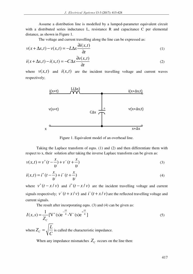
Assume a distribution line is modelled by a lumped-parameter equivalent circuit

with a distributed series inductance L, resistance R and capacitance C per elemental

distance, as shown in Figure 1.

The voltage and current travelling along the line can be expressed as:

( , )( , ) ( , )

i x tv x x t v x t L x

t

∂+ ∆ − = − ∆

∂ (1)

( , )( , ) ( , )

v x ti x x t i x t C x

t

∂+ ∆ − = − ∆

∂ (2)

where ( , )v x t

and ( , )i x t

are the incident travelling voltage and current waves

respectively;

Figure 1. Equivalent model of an overhead line.

Taking the Laplace transform of eqns. (1) and (2) and then differentiate them with

respect to x, their solution after taking the inverse Laplaec transform can be given as:

( , ) ( ) ( )x x

v x t v t v tυ υ

+ −= − + + (3)

( , ) ( ) ( )x x

i x t i t i tυ υ

+ −= − + + (4)

where ( / )v t x v+ − and ( / )i t x v

+ − are the incident travelling voltage and current

signals respectively; ( / )v t x v− + and ( / )i t x v

− + are the reflected travelling voltage and

current signals.

The result after incorporating eqns. (3) and (4) can be given as:

1( , ) [V (s)e -V (s)e ]

sx sx

C

I x sZ

υ υ− +

+ −= (5)

where C

LZ

C= is called the characteristic impedance.

When any impedance mismatches CZ occurs on the line then:

+

i(x+t) L(∆x)

i(x+∆x,t)

v(x+t) v(x+∆x,t)

x+∆x

C∆x

x


418

( , ) ( ) ( , )R

V l s Z s I l s= (6)

Solving for ( , )V l s−

from eqns. (5) and (6):

2( , ) ( ) ( ) sV l s s V s e

τ− + −= Γ (7)

where R C

R C

Z Z

Z Z

−Γ =

+

is called the receiving end voltage reflection coefficient; l

τυ

= is

the transit time.

The TDR method using a single pulse for fault diagnosis is imprecise due to

stimulus attenuation with fault distance and phase change distortion with frequency [22-

23]. To overcome the disadvantages of the traditional TDR method, instead of using single

pulse, a PRBS perturbation is inputted into the line under test for the purpose of finding the

fault as shown in Figure 2. Then echo responses of this pulse energy are cross-correlated

with the incident PRBS by the following formula:

1

1( ) ( ) ( )

L

xy

i

C k x i y i kL =

= +∑ (8)

where Cxy is cross-correlation (CCR) function between reflected wave and incident wave; xi

is the forward signal and yi is the feedback signal. In this paper, the CCR along with the

reflected signals obtained from TDR trace are used for SVM training phase for the first

time.

Figure 2. Single-line diagram of a radial distribution system.

2.2. Support vector machine

Support vector machine is one of the most optimal techniques for data classification,

which was first mentioned by Vapnik in 1995 [24]. SVM works based on the structural risk

minimization principle combined with statistical machine learning theory (SLR). The

global optimization and high generalization ability are the main advantages of SVM as

comparing to artificial neuron network (ANN).

SVM is employed to map the input data (x) into a high-dimensional feature space

and build an optimal hyperplane to separate samples from two classes. To build the optimal

hyperplane, the quadratic optimization equation has to be solved:

Min: 2

2

1

1|| w ||

2

m

i

i

C ξ=

+ ∑ (9)

SS

LOAD

R PRBS


419

Subjec to: ( )w 1 , 0, 1,...,i i i iy x b i mξ ξ× + ≥ − ≥ = (10)

where xi ∈ Rn are feature vectors, yi ∈ (-1,+1) are label vectors, C is the regularization

parameter and ξi is the penalizing relaxation variables.

Equation (10) ensures that:

w ( ) 1i

x bφ× + ≥ + if 1i

y = + (11)

w ( ) 1i

x bφ× + ≥ − if 1i

y = − (12)

The nonlinear classifier can be denoted in the input space as:

* *

1

( ) ( ( , ) )m

i i i i

i

f x sign y K x y bα=

= × × +∑ (13)

where f(x) is the decision function, αi the Lagrangian multipliers, *

b is the bias and

( , )i i

K x y is the kernel function.

It can be clearly seen from eqn. (13) that the performance of SVM is dependent on

training samples and kernel function. Thus, it is necessary to select an appropriate kernel

function. In this paper, the following radial basis function (RBF) is used:

( ) ( )2, expK x y x yγ= − − (14)

where γ is the kernel parameter.

To obtain a good performance, some parameters in SVM must be chosen carefully.

These parameters include the regularization parameter C and the kernel function parameter

γ, these two parameters are automatically selected by means of 5-fold cross-validation

method.

Consequently, classification problem plays a major role in various fields of

computer science and engineering. SVM is known as the most optimal technique to solve

this problem. It has a clear and solid theoretical foundation and simple structure to employ.

Furthermore, SVM is a strongly regularized method, which is suitable for classification

problem. It unfolds a unique technique with small training time.

2.3. Classical multidimensional scaling

For mentioned approach, various TDR responses are recorded, in which there are

some irrelevant data that may be confusing to the SVM classifier and increase the training

time. Feature extraction is the most effective method to select appropriate input features in

order to improve the speed of training and the success rate of classification. Principle

component analysis (PCA) [25], singular value decomposition (SVD) [26] and

multidimensional scaling (MDS) have been widely applied to remove redundant variables

in feature vectors [27]. In this article, classical multidimensional scaling (CMDS) is

employed to select optimal features in order to provide a reliable dataset for the SVM

classifier. It is a nonlinear optimization technique to yield a lower dimensional

representation of high dimensional data. The detail of CMDS feature extraction method has

been well studied in [28-29].

Suppose having a collection of n subjects, the pair-wise distance matrix is given as:


420

11 12 1

21 22 2

31 32 3

n

n

n

δ δ δ

δ δ δ

δ δ δ

∆ =

K

K

K

(15)

where ijδ is the distance between i

x and jx .

The aim of CMDS is to find n vector 1 2, ,...,n L

x x x R∈ to minimize a loss

function called STRAIN. The STRAIN is defined as follows;

( )

1/22

ij

2

ij

( ( , ) )i j

i j

i j

b x x

S Xb

<

<

−

=

∑

∑ (16)

where ijb are the terms of the inner product B ,

11 12 1

'

21 22 2

31 32 3

*

n

n

n

b b b

B X X b b b

b b b

= =

K

K

K

(17)

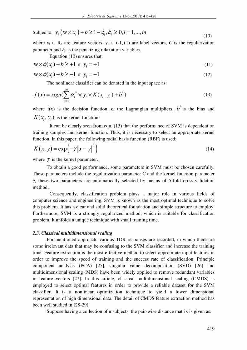
3. Development of Methodology

Since TDR technology alone is not able to diagnosis the fault in distribution

networks and hence requires pattern recognition techniques to support it. In this work, a

CMDS-based SVM classifier is applied to improve the performance of TDR method in

identifying fault types in radial distribution systems. Figure 3 shows the overall structure of

the proposed approach.

Figure 3. The overall structure of the proposed algorithm.

Reflected data

acquisition or

dataset

Feature

extraction

by CMDS

Training

dataset

Testing

dataset

SVM1

SVM2

AG

BG

CG

AB

AC

BC

SVM8 ABG

ACG

BCG

SVM9 ABC


421

The “one to others” SVM algorithm has developed for the multi-class fault

identifier. Nine layers SVM are employed to classify all 10 types of short circuit faults.

When the input of SVM is an AG sample, the output of SVM1 is set to +1; otherwise -1.

With samples of the remain faulty group, SVM2 is trained to separate BG fault from eight

types of short circuit fault, the output of SVM2 is set to +1, otherwise -1, and so on.

Therefore, it can be seen that the multilayer SVM classifier is obtained with all sub-

classifiers.

3.1. Data descriptions

Whenever a fault occurs in distribution networks, the reflected responses will be

produced and travel between fault location and the substation. Note that the magnitude of

reflected responses is proportional to the fault distance from the substation. By increasing

fault distance, the amplitude attenuation along the line increases and so the magnitude of

reflected signals goes down. These fault responses are cross-correlated with the incident

impulse by eqn. (8) as mentioned above. On the other hand, the magnitude of feedback

wave changes for the different fault types, as a result, the peaks of CCR between reflected

signal and incident signals are not the same for each of fault type.

Based on the above analysis, the reflected voltage and current magnitude along

with the peaks of CCR are chosen as the input feature vectors of the SVM classifier, and

the corresponding fault type is chosen as the output. Therefore, the total number of features

is 12, in which six features are the reflected voltage and current values available at the

substation and the remaining six features are the peaks of CCR functions between reflected

and incident waves.

3.2. Feature selection

For classification problems, feature extraction plays a major role in removing

redundant one which can ambiguities for classification in order to increase the training

speed and improve the classification accuracy. In this paper, CMDS algorithm is introduced

for selecting required features as discussed in Section 2. The experimental results show that

CMDS is used to find 6 best optimal features and lead to reduce the training time and the

classification error with the lower feature space dimension.

3.3. Training phase

The SVM classifier is trained using eqns. (9) and (10). The RBF in equation (14) is

chosen as a kernel function, where C is the penalty parameter of the error term and γ is

kernel parameter. These two parameters are selected using the 5-fold cross-validation

method in which the training set is classified into 5 subsets with equal size. After that, each

subset is tested using the classifier trained on the remaining 4 subsets. Therefore, each case

of the training set is identified once, as a result, the classification accuracy is the percentage

of data that are correct classified. The main advantage of cross-validation is the capacity of

removing the overfitting problem. Furthermore, a “grid-search” on C and γ using cross-

validation are employed in this article. As a result, the best cross-validation accuracy is

selected from various couple (C, γ) values are tried.


422

3.4. Testing phase

As the performance of the validation dataset starts to separate from that of the

training dataset, learning procedure is stopped. After the training phase, new patterns of the

testing dataset are inputted to the trained multilayer SVM classifier for purpose of

identifying ten types of fault.

3.5. The output of SVM classifier

The types of fault divided into the following categories: single-phase-to-ground fault

(AG, BG, CG), line-to-line fault (AB, AC, BC), double-line-to-ground fault (ABG, ACG,

BCG) and three-phase fault (ABC).

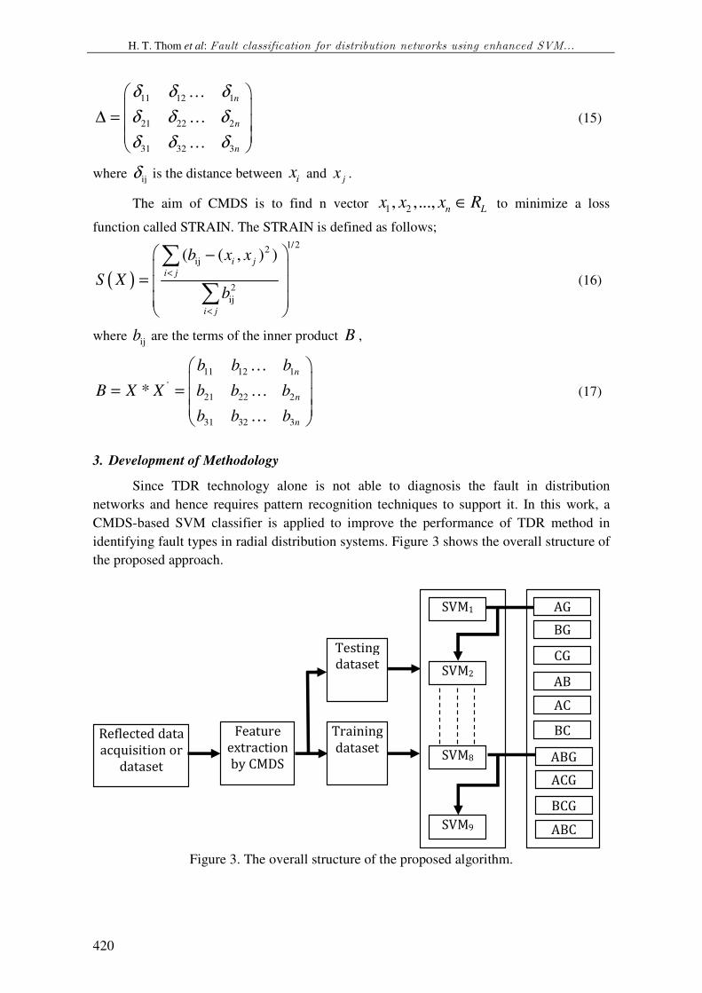
4. Results and discussion

The proposed fault diagnosis method is used to analyze various faults classification

on a simple two-branched distribution system shown in Figure 4. It is constructed from

major components such as conductors, distribution transformers and loads.

Figure 4. Modeling of a typical two-branched distribution network.


423

Figure 5. The waveform of PRBS exciation on the line.

In this paper, the fault types are considered using a 127 bit PRBS input given in

Figure 5 with the frequency f = 1MHz propagating along the line with the velocity of

198,000 km/s. When a fault occurs on the main feeder or on a lateral, an input pattern can

be obtained at substation by TDR analysis. After that, each type of fault can be identified

by the SVM classifier which has been trained earlier.

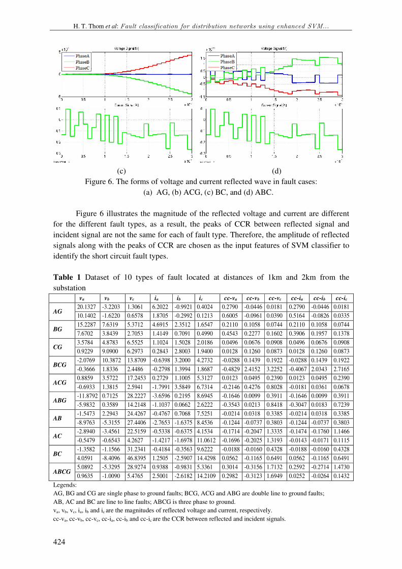
Figure 6 shows TDR curves of voltage and current, generated by simulation of some

types of fault of AG, ACG, BC and ABC on the first lateral, locate at distance of 2 km from

the substation.

(a) (b)


424

(c) (d)

Figure 6. The forms of voltage and current reflected wave in fault cases:

(a) AG, (b) ACG, (c) BC, and (d) ABC.

Figure 6 illustrates the magnitude of the reflected voltage and current are different

for the different fault types, as a result, the peaks of CCR between reflected signal and

incident signal are not the same for each of fault type. Therefore, the amplitude of reflected

signals along with the peaks of CCR are chosen as the input features of SVM classifier to

identify the short circuit fault types.

Table 1 Dataset of 10 types of fault located at distances of 1km and 2km from the

substation

va vb vc ia ib ic cc-va cc-vb cc-vc cc-ia cc-ib cc-ic

AG 20.1327 -3.2203 1.3061 6.2022 -0.9921 0.4024 0.2790 -0.0446 0.0181 0.2790 -0.0446 0.0181

10.1402 -1.6220 0.6578 1.8705 -0.2992 0.1213 0.6005 -0.0961 0.0390 0.5164 -0.0826 0.0335

BG 15.2287 7.6319 5.3712 4.6915 2.3512 1.6547 0.2110 0.1058 0.0744 0.2110 0.1058 0.0744

7.6702 3.8439 2.7053 1.4149 0.7091 0.4990 0.4543 0.2277 0.1602 0.3906 0.1957 0.1378

CG 3.5784 4.8783 6.5525 1.1024 1.5028 2.0186 0.0496 0.0676 0.0908 0.0496 0.0676 0.0908

0.9229 9.0900 6.2973 0.2843 2.8003 1.9400 0.0128 0.1260 0.0873 0.0128 0.1260 0.0873

BCG -2.0769 10.3872 13.8709 -0.6398 3.2000 4.2732 -0.0288 0.1439 0.1922 -0.0288 0.1439 0.1922

-0.3666 1.8336 2.4486 -0.2798 1.3994 1.8687 -0.4829 2.4152 3.2252 -0.4067 2.0343 2.7165

ACG 0.8859 3.5722 17.2453 0.2729 1.1005 5.3127 0.0123 0.0495 0.2390 0.0123 0.0495 0.2390

-0.6933 1.3815 2.5941 -1.7991 3.5849 6.7314 -0.2146 0.4276 0.8028 -0.0181 0.0361 0.0678

ABG -11.8792 0.7125 28.2227 -3.6596 0.2195 8.6945 -0.1646 0.0099 0.3911 -0.1646 0.0099 0.3911

-5.9832 0.3589 14.2148 -1.1037 0.0662 2.6222 -0.3543 0.0213 0.8418 -0.3047 0.0183 0.7239

AB -1.5473 2.2943 24.4267 -0.4767 0.7068 7.5251 -0.0214 0.0318 0.3385 -0.0214 0.0318 0.3385

-8.9763 -5.3155 27.4406 -2.7653 -1.6375 8.4536 -0.1244 -0.0737 0.3803 -0.1244 -0.0737 0.3803

AC -2.8940 -3.4561 22.5159 -0.5338 -0.6375 4.1534 -0.1714 -0.2047 1.3335 -0.1474 -0.1760 1.1466

-0.5479 -0.6543 4.2627 -1.4217 -1.6978 11.0612 -0.1696 -0.2025 1.3193 -0.0143 -0.0171 0.1115

BC -1.3582 -1.1566 31.2341 -0.4184 -0.3563 9.6222 -0.0188 -0.0160 0.4328 -0.0188 -0.0160 0.4328

4.0591 -8.4096 46.8395 1.2505 -2.5907 14.4298 0.0562 -0.1165 0.6491 0.0562 -0.1165 0.6491

ABCG 5.0892 -5.3295 28.9274 0.9388 -0.9831 5.3361 0.3014 -0.3156 1.7132 0.2592 -0.2714 1.4730

0.9635 -1.0090 5.4765 2.5001 -2.6182 14.2109 0.2982 -0.3123 1.6949 0.0252 -0.0264 0.1432

Legends:

AG, BG and CG are single phase to ground faults; BCG, ACG and ABG are double line to ground faults;

AB, AC and BC are line to line faults; ABCG is three phase to ground.

va, vb, vc, ia, ib and ic are the magnitudes of reflected voltage and current, respectively.

cc-va, cc-vb, cc-vc, cc-ia, cc-ib and cc-ic are the CCR between reflected and incident signals.


425

Through simulation 5700 input dataset have been generated by creating various

faults at different locations on two laterals with varying fault impedance value. Training

and testing set are randomly separated from these datasets. 4500 and 1200 datasets are used

for training and testing set respectively.

Table 1 gives some samples of the dataset, generated by simulating all 10 types of

fault on the first lateral, locate at distances of 1km and 2km from the substation for brevity.

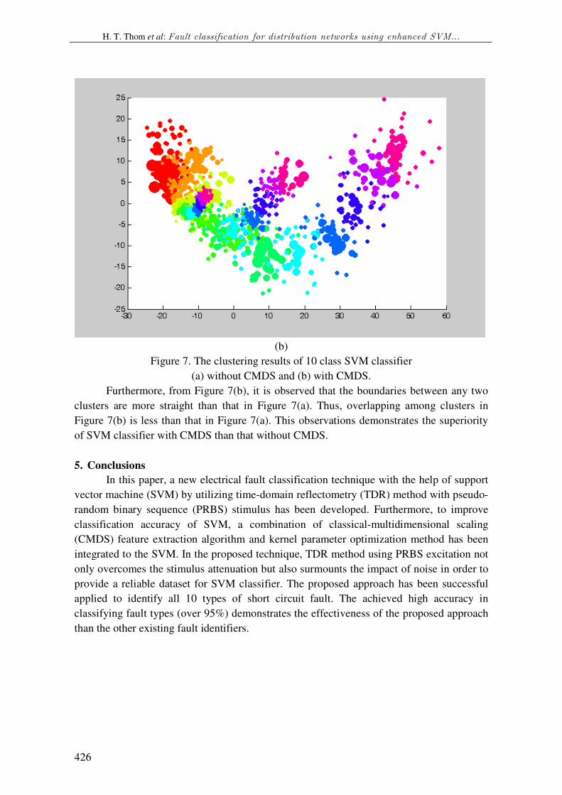
Table 2 gives the results of the classification accuracy whereas Figure 7 shows all

the 10 clusters of the classified fault types for SVM algorithm using dataset with and

without CMDS feature extraction.

Table 2 The results of SVM classification with and without considering CMDS

optimization techniques

SVM classifier No. of

features C γ

Classification accuracy

(%) Training time (s)

Without CMDS 12 181.0193 1.1212 93.00 63.54

With CMDS 6 20.7494 9.7814 95.25 34.18

From Table 2, it is observed that the optimum values of C and γ of SVM classifier

are 181.0193 and 1.1212 without considering CMDS and are 20.7494 and 9.7814 with

considering CMDS. It is clearly seen from this table that the classification accuracy in the

case of using all the feature is 93% whereas this percentage is 95.25% after using CMDS

feature extraction. It can be observed that the overall training time taken by SVM classifier

without CMDS is 63.54 sec whereas with CMDS is 34.18 sec. Thus, it can be concluded

that the proposed CMDS method is not only capable of improving classification accuracy,

but also increasing the training speed.

(a)


426

(b)

Figure 7. The clustering results of 10 class SVM classifier

(a) without CMDS and (b) with CMDS.

Furthermore, from Figure 7(b), it is observed that the boundaries between any two

clusters are more straight than that in Figure 7(a). Thus, overlapping among clusters in

Figure 7(b) is less than that in Figure 7(a). This observations demonstrates the superiority

of SVM classifier with CMDS than that without CMDS.

5. Conclusions

In this paper, a new electrical fault classification technique with the help of support

vector machine (SVM) by utilizing time-domain reflectometry (TDR) method with pseudo-

random binary sequence (PRBS) stimulus has been developed. Furthermore, to improve

classification accuracy of SVM, a combination of classical-multidimensional scaling

(CMDS) feature extraction algorithm and kernel parameter optimization method has been

integrated to the SVM. In the proposed technique, TDR method using PRBS excitation not

only overcomes the stimulus attenuation but also surmounts the impact of noise in order to

provide a reliable dataset for SVM classifier. The proposed approach has been successful

applied to identify all 10 types of short circuit fault. The achieved high accuracy in

classifying fault types (over 95%) demonstrates the effectiveness of the proposed approach

than the other existing fault identifiers.


427

References [1] J. Mora-Flórez, J. Cormane-Angarita and G. Carrillo-Caicedo, “Algorithm And Mixture Distributions For

Locating Faults In Power Systems,” Electric Power System Research, 79: pp. 714-721, 2009.

[2] M. Mirzaei, H. Hizam and M. Z. A. AbKadir, “Review of fault location methods for distribution power

system, ”Australian Journal of Basic and Applied Sciences, 3: pp. 2670-2676, 2009.

[3] E. C. Senger, G. Manassero Jr., C. Goldemberg and E. L. Pellini, “automated fault location system for

primary distribution networks,” IEEE Trans on Power Delivery, 20: pp. 1332-1340, 2005.

[4] F. H. Magnago and A. Abur, “fault location using wavelets,” IEEE Transactions on Power Delivery, Vol.

13, No. 4, pp. 1475-1480, October 1998.

[5] A. Borgheti, S. Corsi, C. A. Nucci, M. Paolone, L. Pereto and R. Tinarelli, “On the use of continuous-

wavelet transform for fault location in distribution power systems,” Electrical Power and Energy Systems,

28: pp. 608-617, 2006.

[6] Z. E. Aygen, S. Seker, M. Bagriyanik and E. Ayaz, “Fault Section estimation in electrical power systems

using artificial neural networks approach,” IEEE Trans. Power Delivery, pp. 466-469, 1999.

[7] M. Al-Shaher, M. M. Sabra and A. S. Saleh, “fault location in multi-ring distribution network using

artificial neural network,” Electric Power Systems Research, 64: pp. 87-92, 2003.

[8] M. Pourahmadi-Nakhli and A. A. Safavi, “Path characteristic frequency-based fault locating in radial

distribution systems using wavelets and neuron networks,” IEEE Trans. Power Delivery, Vol. 60, pp. 1654-

1663, 2011.

[9] J. J. Mathew and A. Francis, “HVDC transmission line fault location using wavelet feeded neural network

bank,” Science Technology & Engineering, Vol. 2, Issue 11, pp. 1-6, 2013.

[10] J. Zhang, Z. Y. He, S. Lin, Y. B. Zhang and Q. Q. Qian, “An ANFIS-based fault classification approach in

power distribution system,” Electrical Power and Energy Systems 49: pp. 243–252, 2013.

[11] P. F. Gale, “Cable fault location by impulse current method,” Proc. IEE, vol. 122, no. 4, pp. 403–408, Apr.

1975.

[12] J. P. Steiner, W. L. Weeks and H. W. Ng, “An automated fault locating system,” IEEE Trans. on Power

Delivery, vol. 7, no. 2, pp. 967–978, Apr. 1992.

[13] G. B. Ancell and N. C. Pahalawaththa, “Effects of frequency dependence and line parameters on single-

phase ended traveling wave based fault location,” IEE Proceedings-C, vol. 139, no. 4, pp. 332–342, July

1992.

[14] K. K. Kuan and K. Warwick, “Real-time expert system for fault location on high voltage underground

distribution cables,” IEE Proceedings-C, vol. 139, no. 3, pp. 235–240, May 1992.

[15] M. Komoda and M. Aihara, “Development of a current detection type cable fault locator,” IEEE Trans. on

Power Delivery, vol. 6, no. 2, pp. 541–545, Apr. 1991.

[16] S. Navaneethan, J. J. Soraghan, W. H. Siew, F. McPherson and P. F. Gale, “Automatic fault location for

underground low voltage distribution networks,” IEEE Transactions on power delivery, Vol. 16, No. 2, pp.

346-351, 2001.

[17] D. M. Horan and R. A. Guinee, “A novel pulse echo correlation tool for transmission path testing and fault

diagnosis,” journal of computers, Vo. l1, No. 1, pp. 31-39, April 2006.

[18] D. Thukaram, H. P. Khincha and H. P. Vijaynarasimha, “Artificial neural network and support vector

machine approach for locating faults in radial distribution systems," IEEE Trans. Power Delivery, Vol. 20,

No. 2, pp. 710-721, 2005.

[19] X. Deng, R. Yuan, Z. Xiao, T. Li and K. L. L. Wanga, “Fault location in loop distribution network using

SVM technology,” Electrical Power and Energy Systems 65: pp. 254–261, 2015.

[20] L. Ye, D. You, X. Yin, K. Wang and J. Wu, “An improved fault-location method for distribution system

using wavelets and support vector regression,” Electrical Power and Energy Systems 55: pp. 467–472,

2014.

[21] X. Zhang, M. Zhang and D. Liu, “Reconstruction of faulty cable network using time domain reflectometry,”

Progress In Electromagnetics Research, Vol. 136, pp. 457-478, 2013.

[22] B. Clegg, Underground Cable Fault Location, McGraw Hill, 1993.

[23] Time Domain Reflectometry Theory, Application Note 1304-2, Agilient Technologies, Aug. 2002,

www.agilient.com.

[24] V. N. Vapnik, “The nature of statistical learning theory” Springer-Verlag, New York, 1995.

[25] S.-F. Yuan and F.-L. Chu, “Support vector machines-based fault diagnosis for turbo-pump rotor”,

Mechanical Systems and Signal Processing 20: pp. 939–952, 2006.


428

[26] M. Kaur, R. Vashisht and N. Neeru, “Recognition of facial expressions with principal component analysis

and singular value decomposition,” International Journal of Computer Applications, Volume 9, No.12, pp.

1-5, November 2010.

[27] Z. Sun and G. Fox, “Traffic flow forecasting based on combination of multidimensional scaling and

SVM,”International Journal of Intelligent Transportation Systems Research January, Volume 12, Issue 1,

pp. 20-25, 2014.

[28] F. W. Young and R. M. Hamer, “Multidimensional scaling: history, theory and applications,” Lawrence

Erlbaum, Hillsdale, NJ, 1987.

[29] I. Borg and P. G. Groenen, “Morden multidimentional scaling,” Springer, New York, 1997.

ming-yuan j. electrical systems 13-3 (2017): 415-428 e cho...

Documents