microstructured optical fiber the design and modeling...
TRANSCRIPT
The design and modeling ofmicrostructured optical fiber
Steven G. Johnson
MIT / Harvard University
Outline
• What are these fibers (and why should I care)?
• The guiding mechanisms: index-guiding and band gaps
• Finding the guided modes
• Small corrections (with big impacts)
Outline
• What are these fibers (and why should I care)?
• The guiding mechanisms: index-guiding and band gaps
• Finding the guided modes
• Small corrections (with big impacts)
protectivepolymersheath
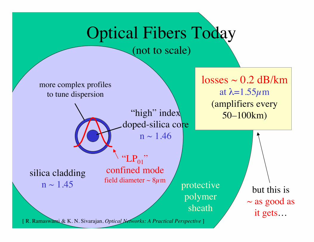
Optical Fibers Today(not to scale)
silica claddingn ~ 1.45
more complex profilesto tune dispersion
“high” indexdoped-silica core
n ~ 1.46
“LP01”confined mode
field diameter ~ 8µm
losses ~ 0.2 dB/kmat λ=1.55µm
(amplifiers every50–100km)
but this is~ as good as
it gets…[ R. Ramaswami & K. N. Sivarajan, Optical Networks: A Practical Perspective ]
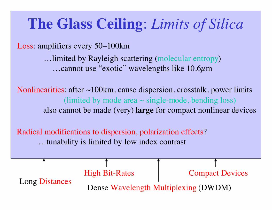
The Glass Ceiling: Limits of Silica
Long DistancesHigh Bit-Rates
Dense Wavelength Multiplexing (DWDM)
Loss: amplifiers every 50–100km
…limited by Rayleigh scattering (molecular entropy)…cannot use “exotic” wavelengths like 10.6µm
Nonlinearities: after ~100km, cause dispersion, crosstalk, power limits(limited by mode area ~ single-mode, bending loss)
also cannot be made (very) large for compact nonlinear devices
Compact Devices
Radical modifications to dispersion, polarization effects?…tunability is limited by low index contrast
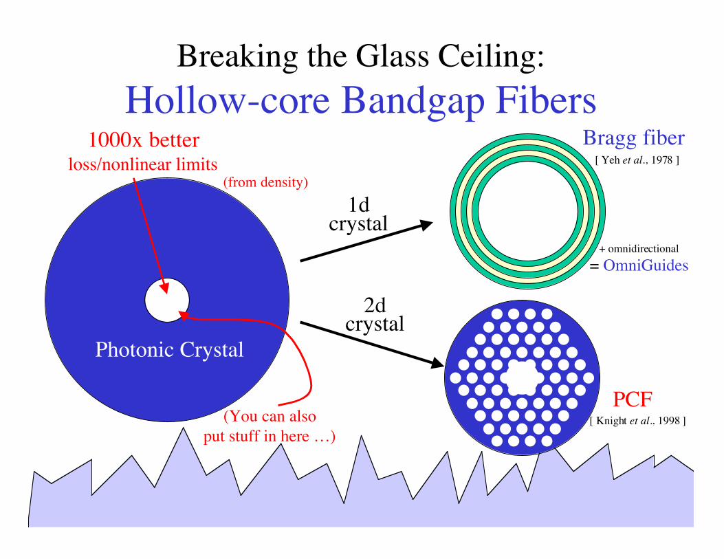
Breaking the Glass Ceiling:Hollow-core Bandgap Fibers
1000x betterloss/nonlinear limits
(from density)
Photonic Crystal
1dcrystal
Bragg fiber[ Yeh et al., 1978 ]
+ omnidirectional
= OmniGuides
2dcrystal
PCF[ Knight et al., 1998 ](You can also
put stuff in here …)
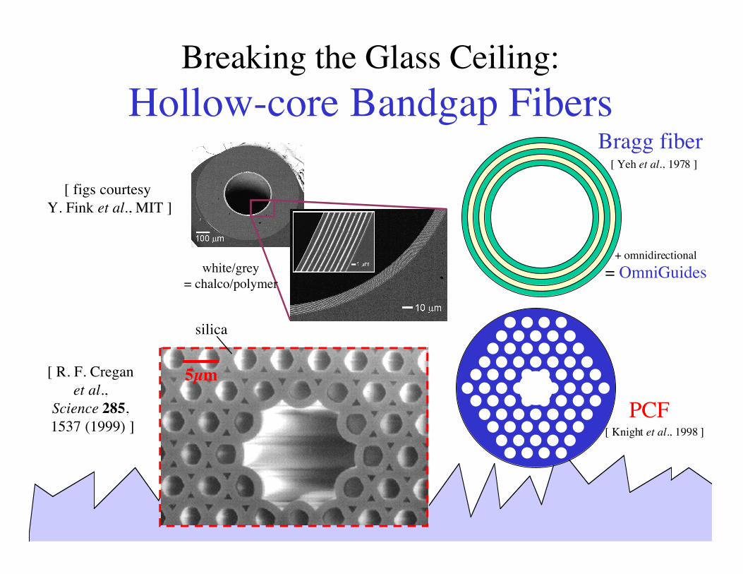
Breaking the Glass Ceiling:Hollow-core Bandgap Fibers
Bragg fiber[ Yeh et al., 1978 ]
+ omnidirectional
= OmniGuides
PCF[ Knight et al., 1998 ]
white/grey= chalco/polymer
5µm[ R. F. Cregan et al.,
Science 285, 1537 (1999) ]
[ figs courtesy Y. Fink et al., MIT ]
silica
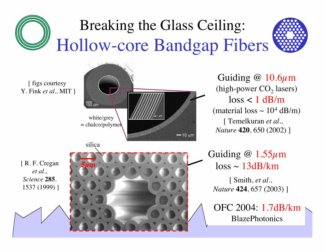
Breaking the Glass Ceiling:Hollow-core Bandgap Fibers
white/grey= chalco/polymer
5µm[ R. F. Cregan et al.,
Science 285, 1537 (1999) ]
[ figs courtesy Y. Fink et al., MIT ]
silica
Guiding @ 10.6µm(high-power CO2 lasers)
loss < 1 dB/m(material loss ~ 104 dB/m)
Guiding @ 1.55µmloss ~ 13dB/km
[ Smith, et al.,Nature 424, 657 (2003) ]
[ Temelkuran et al.,Nature 420, 650 (2002) ]
OFC 2004: 1.7dB/kmBlazePhotonics
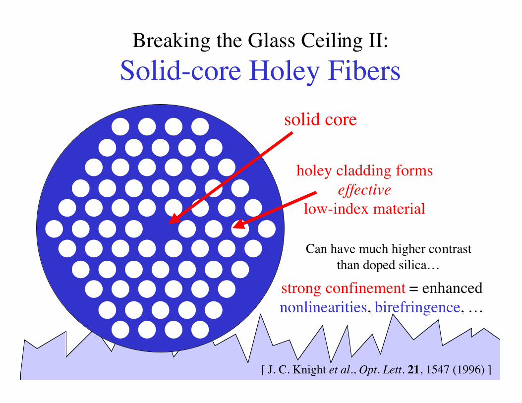
Breaking the Glass Ceiling II:
Solid-core Holey Fibers
solid core
holey cladding formseffective
low-index material
[ J. C. Knight et al., Opt. Lett. 21, 1547 (1996) ]
Can have much higher contrastthan doped silica…
strong confinement = enhancednonlinearities, birefringence, …

Breaking the Glass Ceiling II:
Solid-core Holey Fibers
[ K. Suzuki,Opt. Express 9,
676 (2001) ]
polarization-maintaining
[ Wadsworth et al.,JOSA B 19,
2148 (2002) ]
nonlinear fibers
[ T. A. Birks et al.,Opt. Lett. 22, 961 (1997) ]
endlesslysingle-mode
[ J. C. Knight et al.,Elec. Lett. 34,1347 (1998) ]
low-contrastlinear fiber(large area)
Outline
• What are these fibers (and why should I care)?
• The guiding mechanisms: index-guiding and band gaps
• Finding the guided modes
• Small corrections (with big impacts)
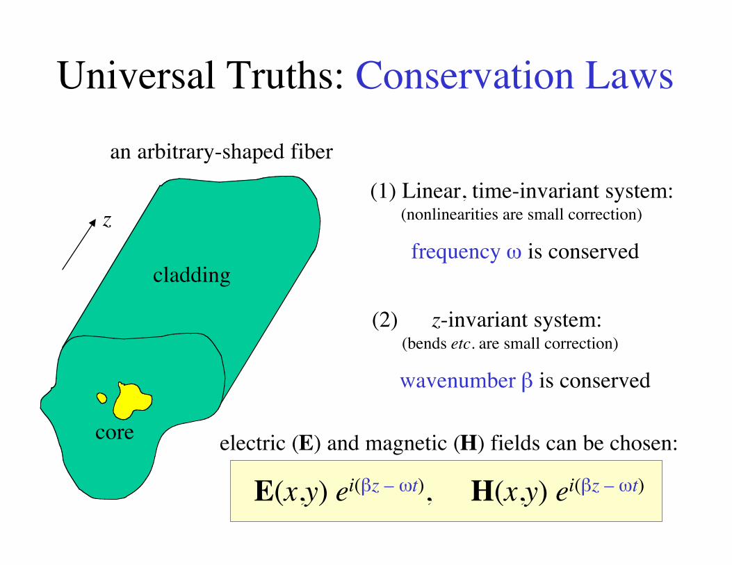
Universal Truths: Conservation Laws
an arbitrary-shaped fiber
z(1) Linear, time-invariant system:
(nonlinearities are small correction)
frequency ω is conserved
(2) z-invariant system: (bends etc. are small correction)
wavenumber β is conserved
electric (E) and magnetic (H) fields can be chosen:
E(x,y) ei(βz – ωt), H(x,y) ei(βz – ωt)
cladding
core
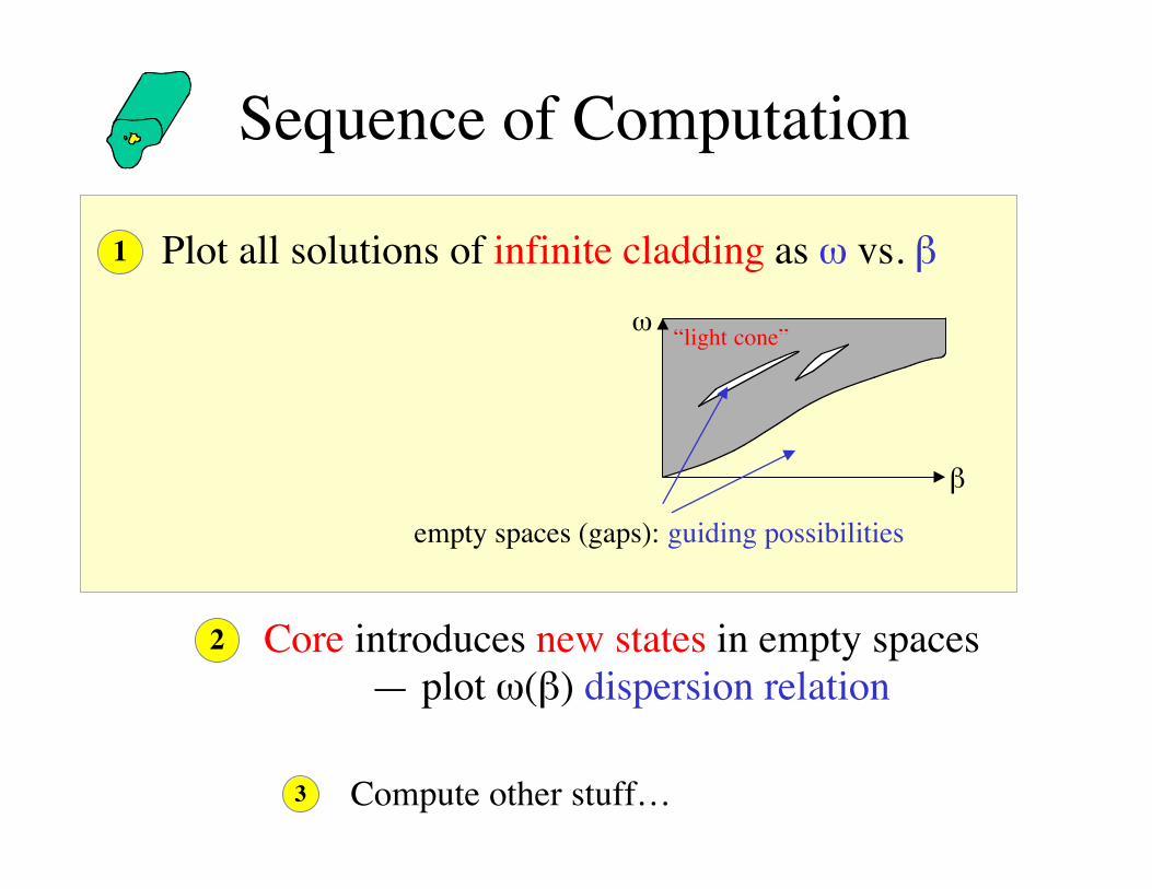
Sequence of Computation
1 Plot all solutions of infinite cladding as ω vs. β
ω
β
empty spaces (gaps): guiding possibilities
2 Core introduces new states in empty spaces— plot ω(β) dispersion relation
3 Compute other stuff…
“light cone”
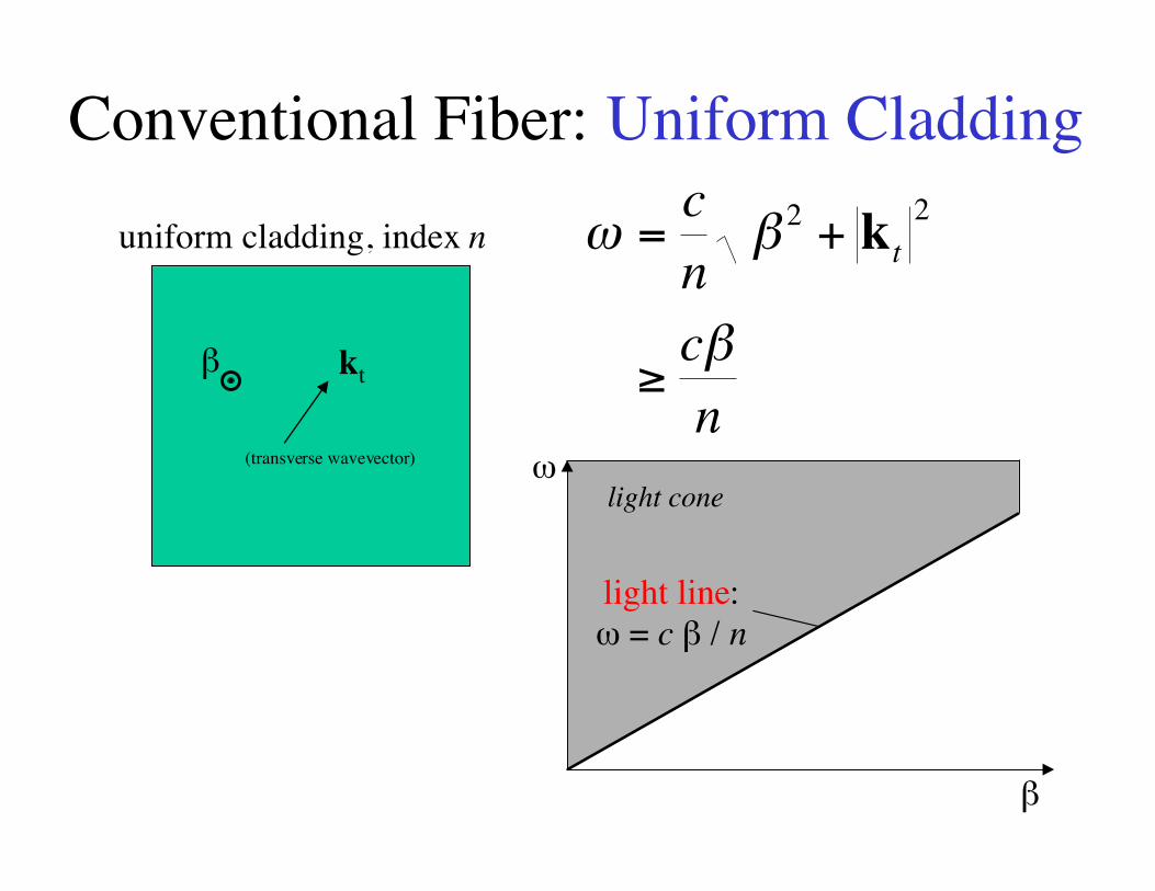
Conventional Fiber: Uniform Cladding
uniform cladding, index n
kt
(transverse wavevector)
ω β
β
= +
≥
cncn
t2 2k
ω
β
light cone
light line:ω = c β / n
β
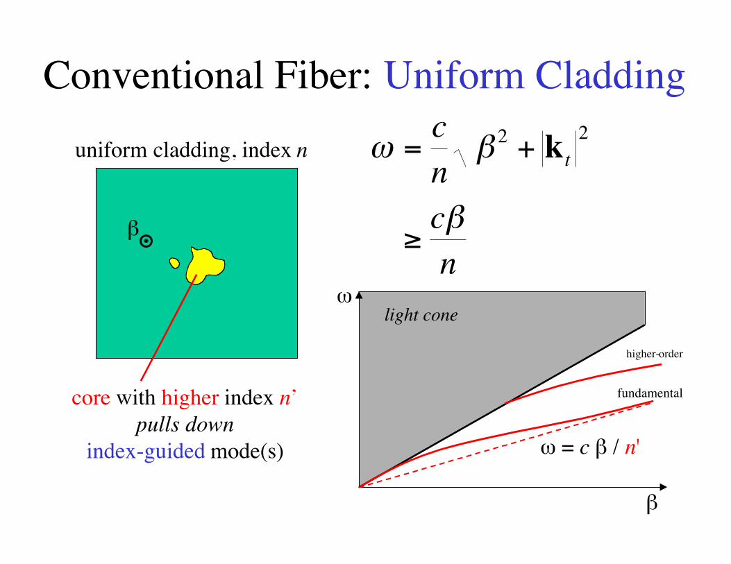
Conventional Fiber: Uniform Cladding
uniform cladding, index n ω β
β
= +
≥
cncn
t2 2k
ω
β
light cone
β
core with higher index n’pulls down
index-guided mode(s) ω = c β / n'
fundamental
higher-order
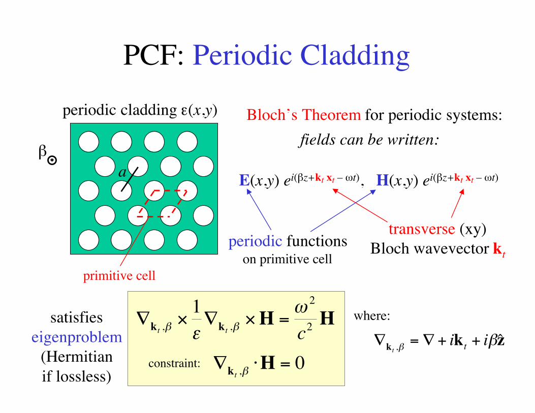
PCF: Periodic Cladding
periodic cladding ε(x,y)
βa
primitive cell
Bloch’s Theorem for periodic systems:
fields can be written:
E(x,y) ei(βz+kt xt – ωt), H(x,y) ei(βz+kt xt – ωt)
periodic functionson primitive cell
transverse (xy)Bloch wavevector kt
∇ = ∇ + +k k zt
i it, ˆβ β∇ × ∇ × =k k H H
t t c, ,β βεω1 2
2
∇ ⋅ =k Ht ,β 0
where:satisfieseigenproblem
(Hermitianif lossless)
constraint:
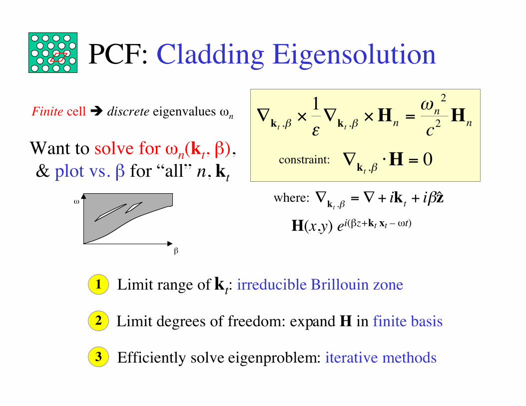
PCF: Cladding Eigensolution
H(x,y) ei(βz+kt xt – ωt)
∇ = ∇ + +k k zt
i it, ˆβ β
∇ × ∇ × =k k H Ht t n
nnc, ,β βε
ω1 2
2
∇ ⋅ =k Ht ,β 0
where:
constraint:
1
Want to solve for ωn(kt, β),& plot vs. β for “all” n, kt
Finite cell � discrete eigenvalues ωn
ω
β
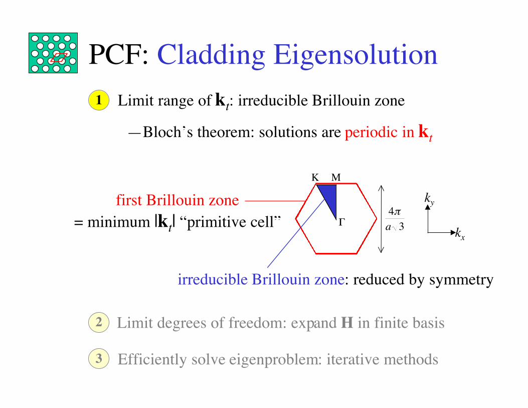
Limit range of kt: irreducible Brillouin zone
2 Limit degrees of freedom: expand H in finite basis
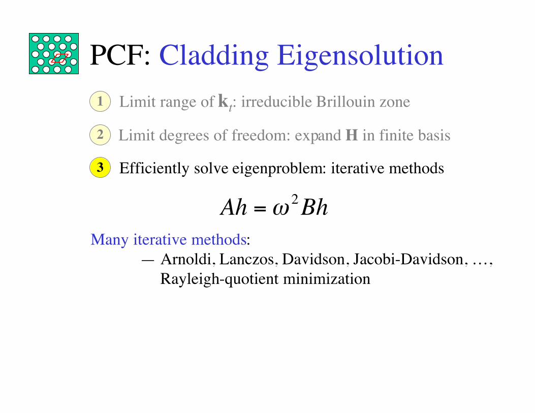
3 Efficiently solve eigenproblem: iterative methods
PCF: Cladding Eigensolution1 Limit range of kt: irreducible Brillouin zone
2 Limit degrees of freedom: expand H in finite basis
3 Efficiently solve eigenproblem: iterative methods
—Bloch’s theorem: solutions are periodic in kt
kx
kyfirst Brillouin zone= minimum |kt| “primitive cell”
43π
aΓ
MK
irreducible Brillouin zone: reduced by symmetry
PCF: Cladding Eigensolution1 Limit range of kt: irreducible Brillouin zone
2 Limit degrees of freedom: expand H in finite basis
3 Efficiently solve eigenproblem: iterative methods
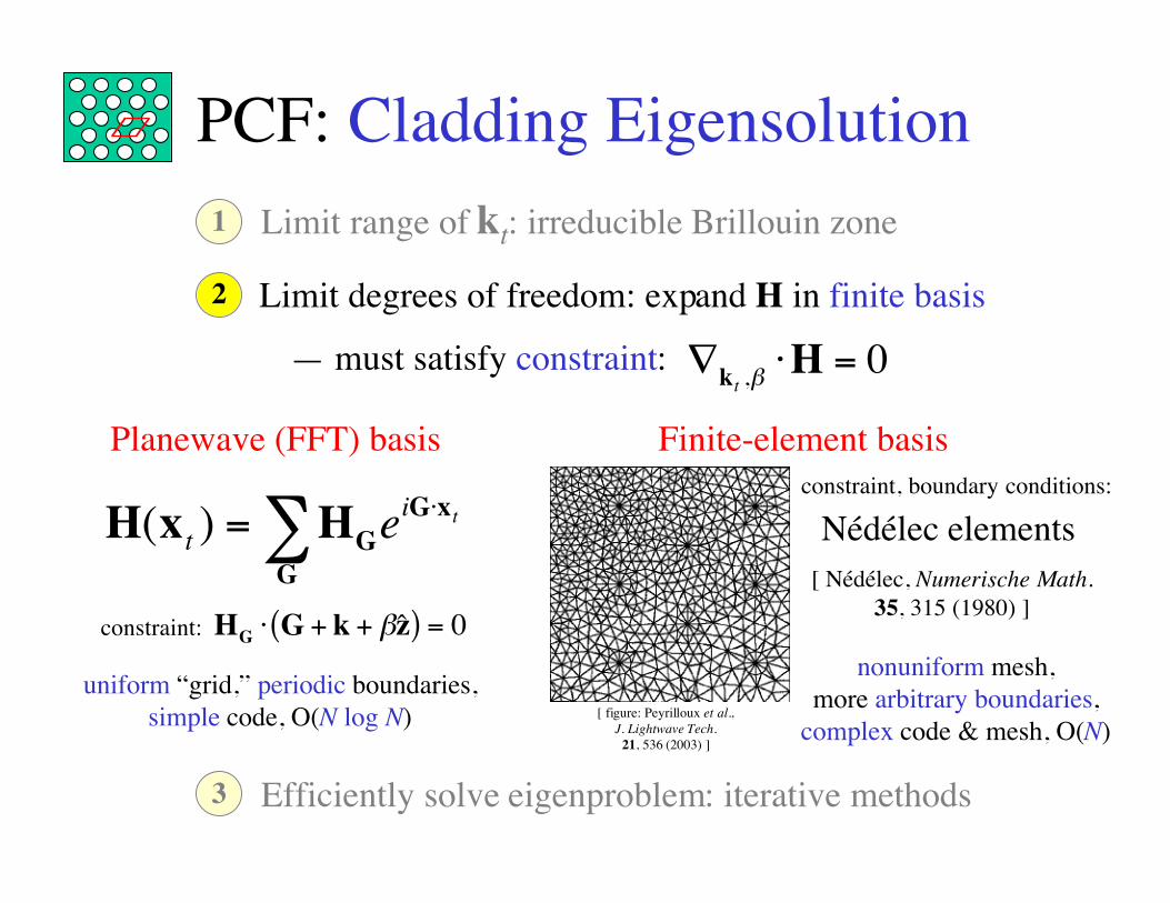
∇ ⋅ =k Ht ,β 0— must satisfy constraint:
Planewave (FFT) basis
H x HGG x
G
( )tie t= ⋅∑
H G k zG ⋅ + +( ) =βˆ 0constraint:
uniform “grid,” periodic boundaries,simple code, O(N log N)
Finite-element basisconstraint, boundary conditions:
Nédélec elements[ Nédélec, Numerische Math.
35, 315 (1980) ]
nonuniform mesh,more arbitrary boundaries,
complex code & mesh, O(N)[ figure: Peyrilloux et al.,
J. Lightwave Tech.21, 536 (2003) ]
PCF: Cladding Eigensolution1 Limit range of kt: irreducible Brillouin zone
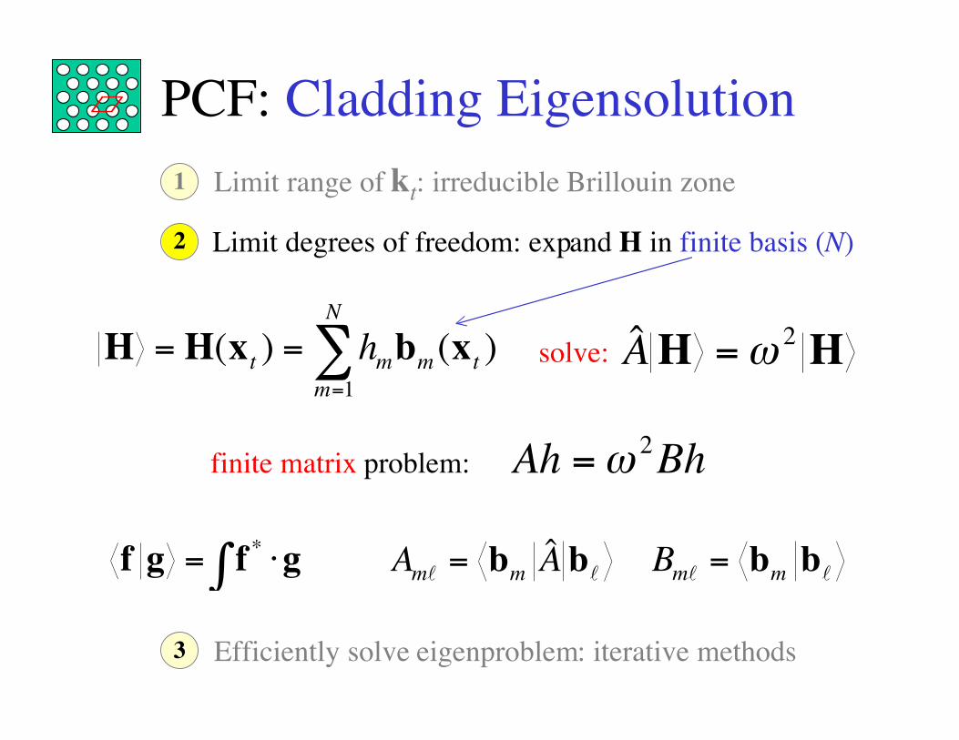
2 Limit degrees of freedom: expand H in finite basis (N)
3 Efficiently solve eigenproblem: iterative methods
H H x b x= ==∑( ) ( )t m m tm
N
h1
solve: A H H=ω 2
Ah Bh=ω 2
A Am ml l= b bˆ Bm ml l= b bf g f g= ⋅∫ *
finite matrix problem:
PCF: Cladding Eigensolution1 Limit range of kt: irreducible Brillouin zone
2 Limit degrees of freedom: expand H in finite basis
3 Efficiently solve eigenproblem: iterative methods
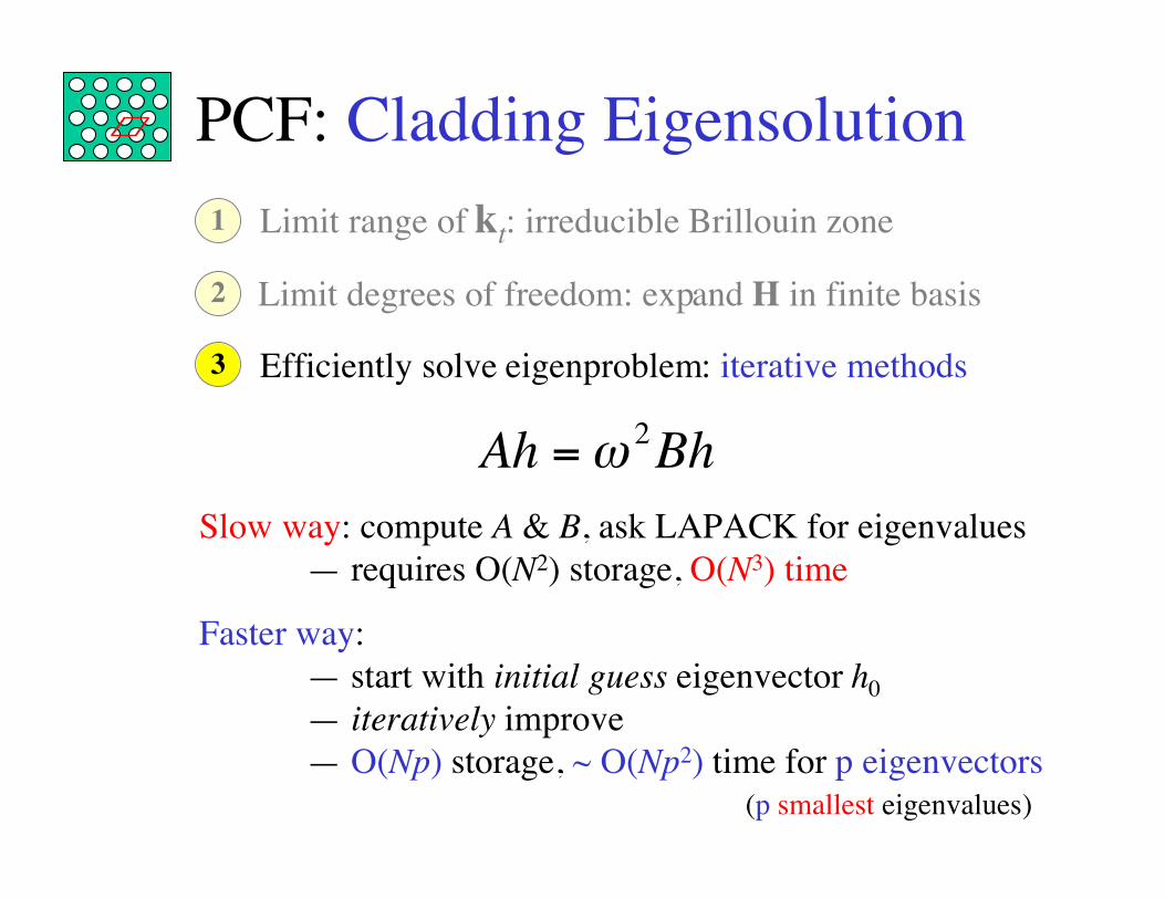
Ah Bh=ω 2
Faster way:— start with initial guess eigenvector h0
— iteratively improve— O(Np) storage, ~ O(Np2) time for p eigenvectors
Slow way: compute A & B, ask LAPACK for eigenvalues— requires O(N2) storage, O(N3) time
(p smallest eigenvalues)
PCF: Cladding Eigensolution1 Limit range of kt: irreducible Brillouin zone
2 Limit degrees of freedom: expand H in finite basis
3 Efficiently solve eigenproblem: iterative methods
Ah Bh=ω 2
Many iterative methods:— Arnoldi, Lanczos, Davidson, Jacobi-Davidson, …, Rayleigh-quotient minimization
PCF: Cladding Eigensolution1 Limit range of kt: irreducible Brillouin zone
2 Limit degrees of freedom: expand H in finite basis
3 Efficiently solve eigenproblem: iterative methods
Ah Bh=ω 2
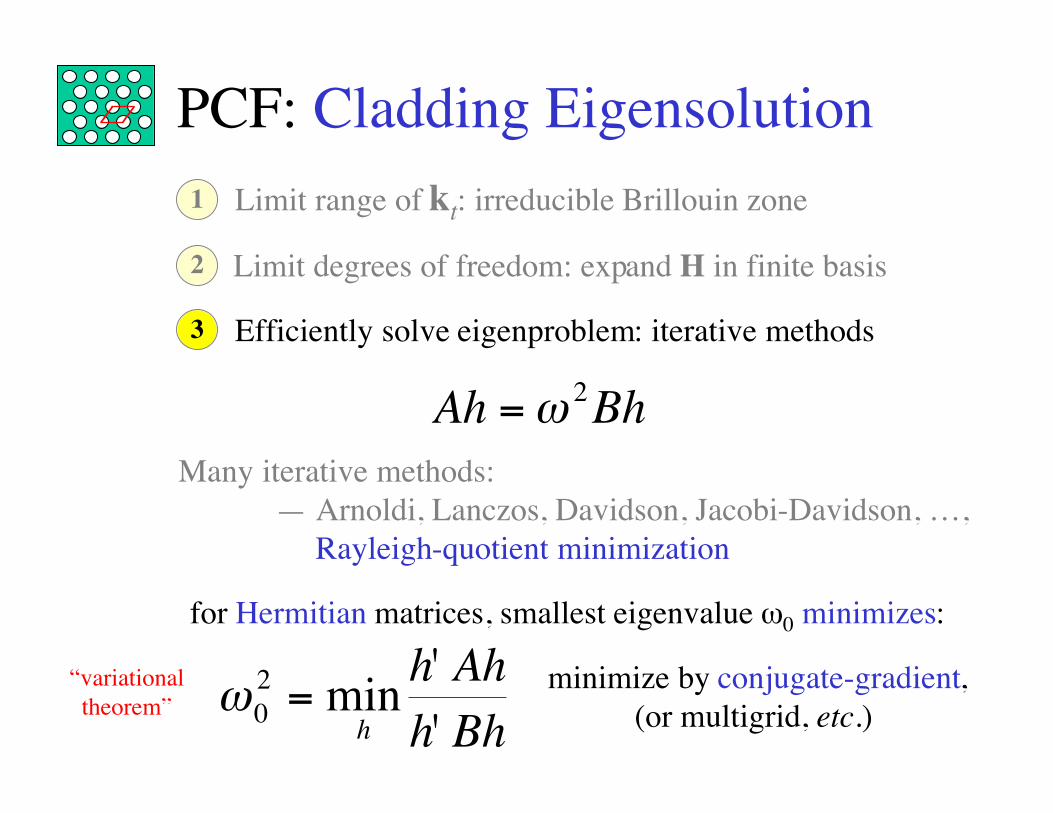
Many iterative methods:— Arnoldi, Lanczos, Davidson, Jacobi-Davidson, …, Rayleigh-quotient minimization
for Hermitian matrices, smallest eigenvalue ω0 minimizes:
ω02 = min
''h
h Ahh Bh
minimize by conjugate-gradient,(or multigrid, etc.)
“variationaltheorem”
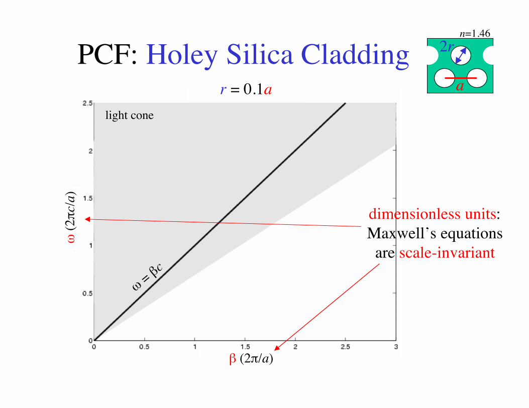
PCF: Holey Silica Cladding 2r
a
n=1.46
β (2π/a)
r = 0.1aω
(2π
c/a)
light cone
ω = βc
dimensionless units:Maxwell’s equations
are scale-invariant

PCF: Holey Silica Cladding 2r
a
n=1.46
β (2π/a)
r = 0.17717aω
(2π
c/a)
light cone
ω = βc
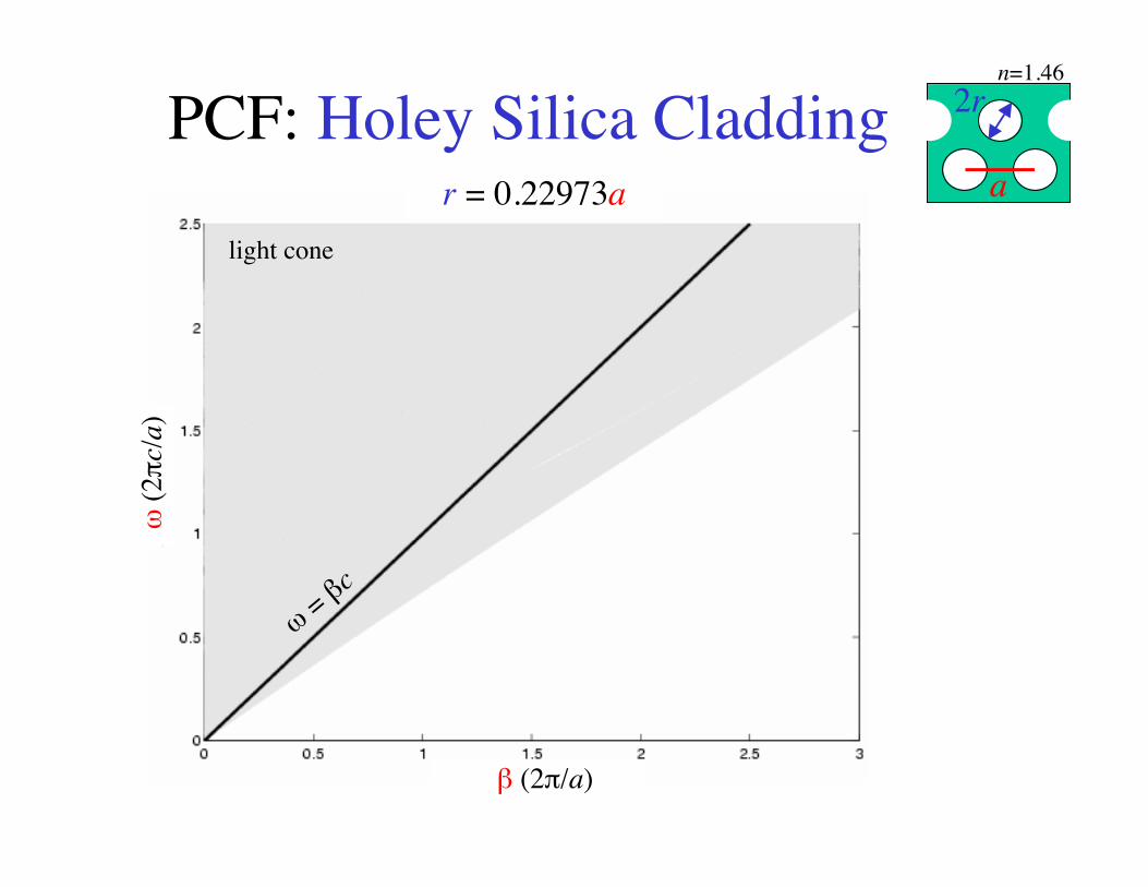
PCF: Holey Silica Cladding 2r
a
n=1.46
β (2π/a)
r = 0.22973aω
(2π
c/a)
light cone
ω = βc
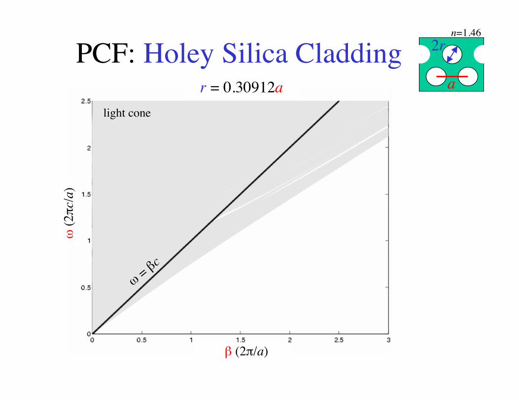
PCF: Holey Silica Cladding 2r
a
n=1.46
β (2π/a)
r = 0.30912aω
(2π
c/a)
light cone
ω = βc

PCF: Holey Silica Cladding 2r
a
n=1.46
β (2π/a)
r = 0.34197aω
(2π
c/a)
light cone
ω = βc

PCF: Holey Silica Cladding 2r
a
n=1.46
β (2π/a)
r = 0.37193aω
(2π
c/a)
light cone
ω = βc

PCF: Holey Silica Cladding 2r
a
n=1.46
β (2π/a)
r = 0.4aω
(2π
c/a)
light cone
ω = βc

PCF: Holey Silica Cladding 2r
a
n=1.46
β (2π/a)
r = 0.42557aω
(2π
c/a)
light cone
ω = βc
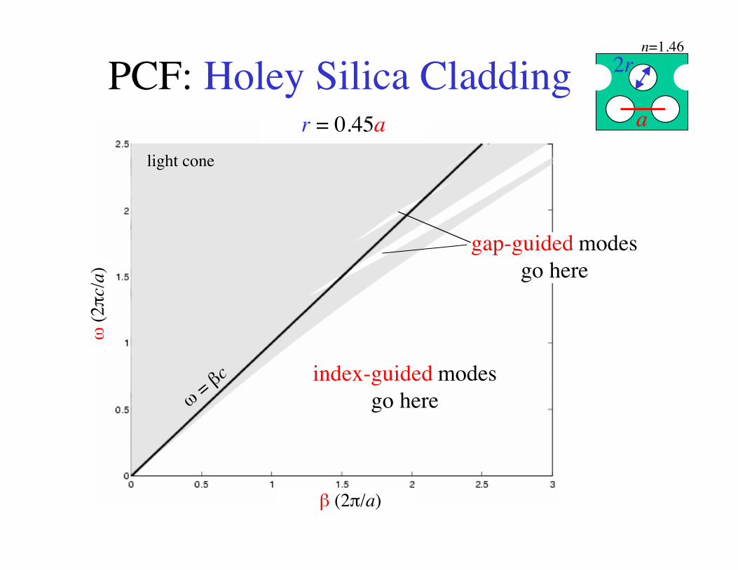
PCF: Holey Silica Cladding 2r
a
n=1.46
β (2π/a)
r = 0.45aω
(2π
c/a)
light cone
ω = βc index-guided modesgo here
gap-guided modesgo here
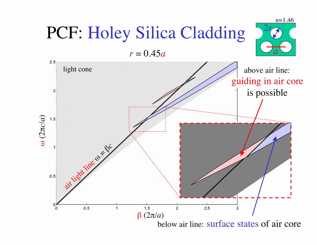
PCF: Holey Silica Cladding 2r
a
n=1.46
β (2π/a)
r = 0.45aω
(2π
c/a)
light cone
air lig
ht lin
e ω = βc
above air line:guiding in air core
is possible
below air line: surface states of air core
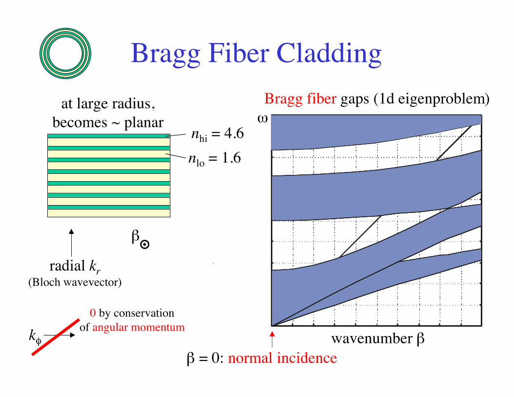
Bragg Fiber Cladding
at large radius,becomes ~ planar
nhi = 4.6
nlo = 1.6
Bragg fiber gaps (1d eigenproblem)
wavenumber β
β
radial kr(Bloch wavevector)
β = 0: normal incidence
kφ
0 by conservationof angular momentum
ω
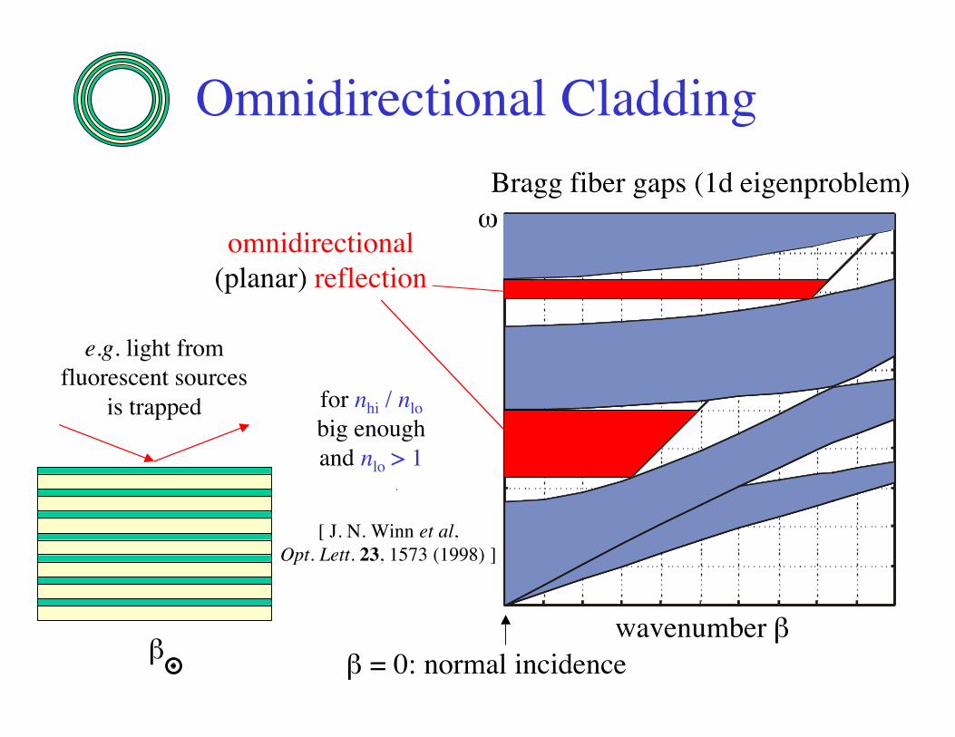
Omnidirectional Cladding
Bragg fiber gaps (1d eigenproblem)
wavenumber ββ β = 0: normal incidence
omnidirectional(planar) reflection
for nhi / nlo
big enoughand nlo > 1
e.g. light fromfluorescent sources
is trapped
[ J. N. Winn et al,Opt. Lett. 23, 1573 (1998) ]
ω
Outline
• What are these fibers (and why should I care)?
• The guiding mechanisms: index-guiding and band gaps
• Finding the guided modes
• Small corrections (with big impacts)
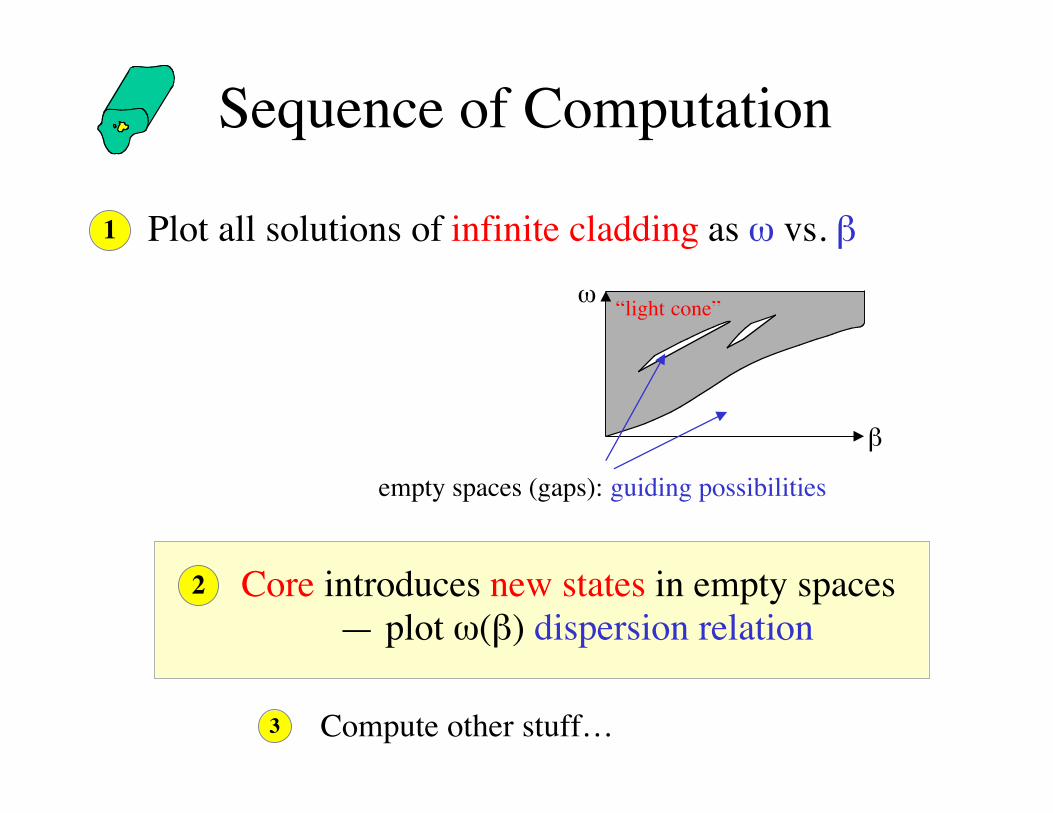
Sequence of Computation
1 Plot all solutions of infinite cladding as ω vs. β
ω
β
empty spaces (gaps): guiding possibilities
2 Core introduces new states in empty spaces— plot ω(β) dispersion relation
3 Compute other stuff…
“light cone”
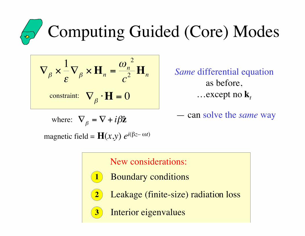
Computing Guided (Core) Modes
magnetic field = H(x,y) ei(βz– ωt)
∇ = ∇ +β βi z
∇ × ∇ × =β βεω1 2
2H Hnn
nc
∇ ⋅ =β H 0
where:
constraint:
Same differential equationas before,
…except no kt
— can solve the same way
1
New considerations:
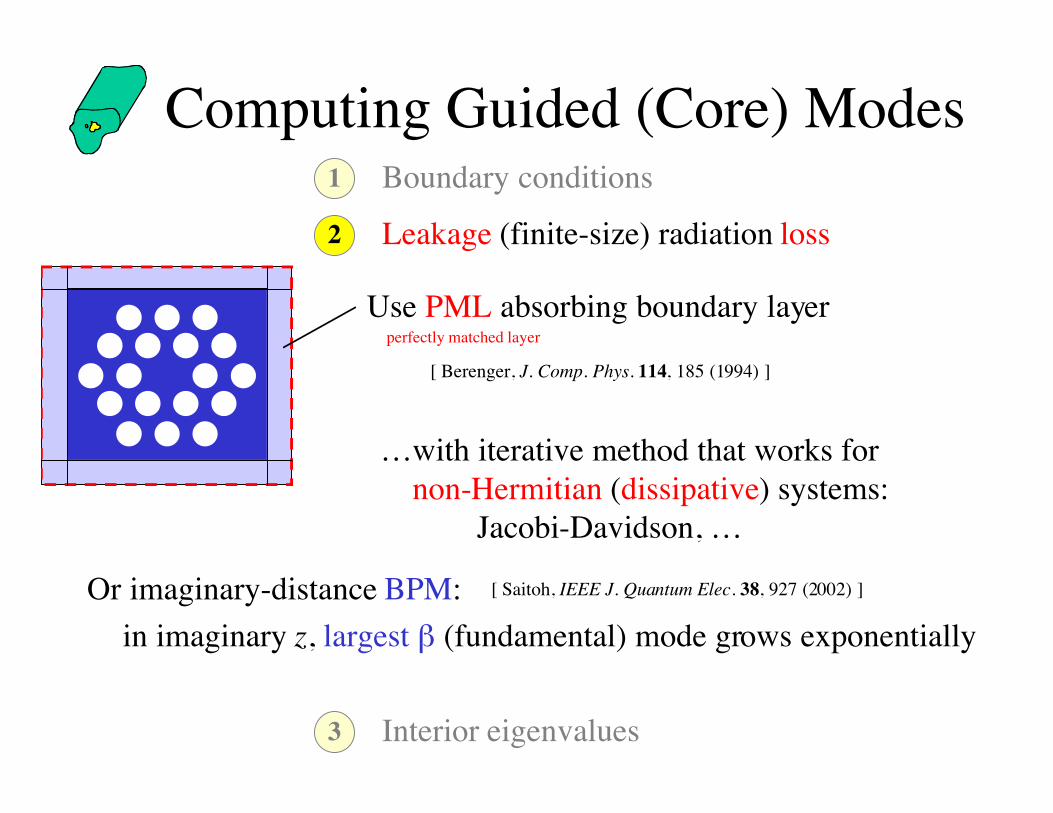
Boundary conditions
2 Leakage (finite-size) radiation loss
3 Interior eigenvalues
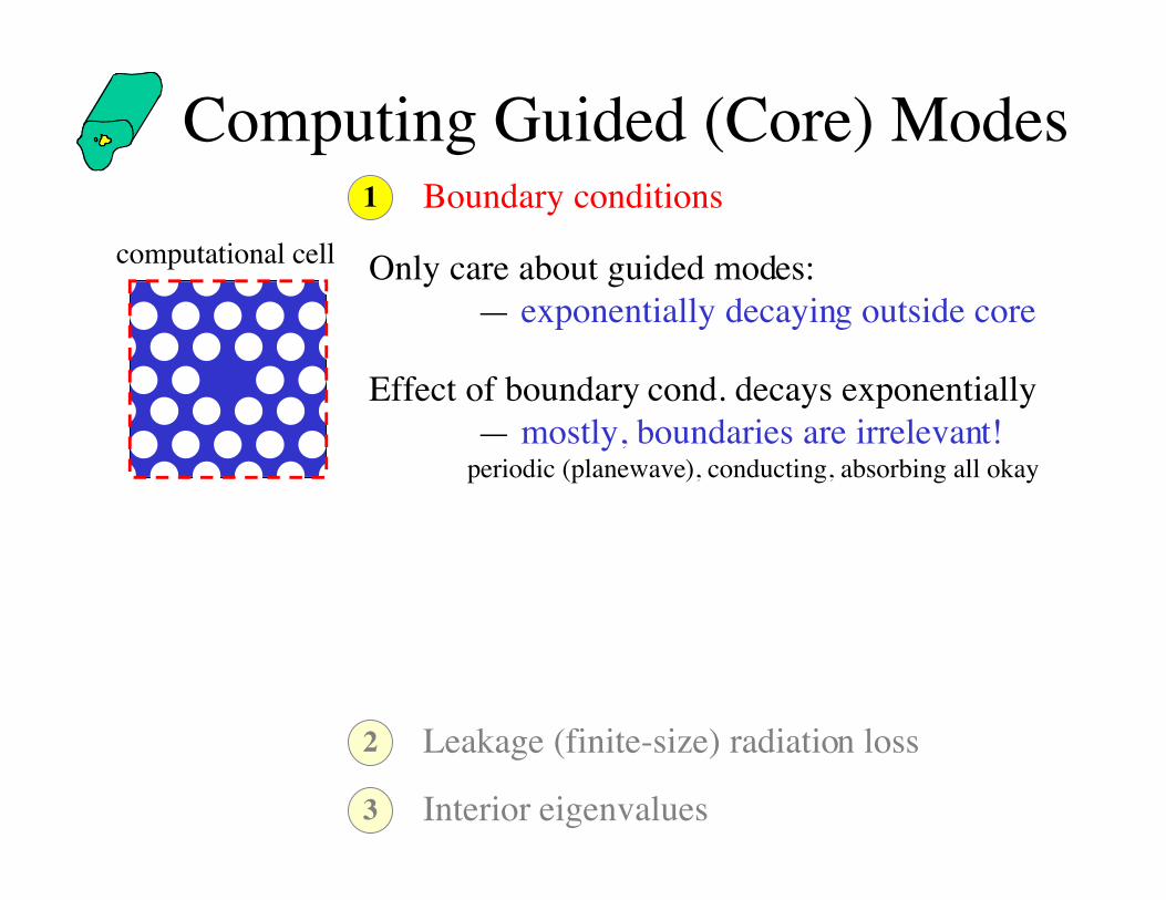
Computing Guided (Core) Modes1 Boundary conditions
2 Leakage (finite-size) radiation loss
3 Interior eigenvalues
Only care about guided modes:— exponentially decaying outside core
computational cell
Effect of boundary cond. decays exponentially— mostly, boundaries are irrelevant!
periodic (planewave), conducting, absorbing all okay
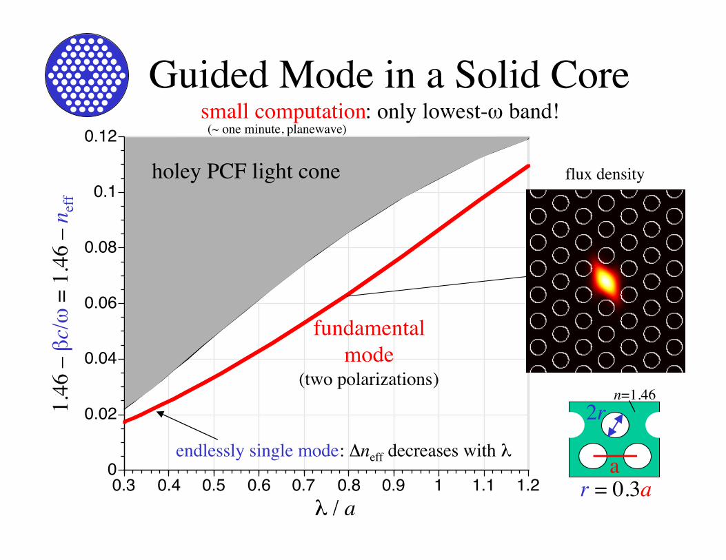
Guided Mode in a Solid Coresmall computation: only lowest-ω band!
0
0.02
0.04
0.06
0.08
0.1
0.12
0.3 0.4 0.5 0.6 0.7 0.8 0.9 1 1.1 1.2
2r
a
n=1.46
r = 0.3a
1.46
– β
c/ω
= 1
.46
– n e
ff
λ / a
holey PCF light cone
fundamentalmode
(two polarizations)
endlessly single mode: ∆neff decreases with λ
flux density
(~ one minute, planewave)
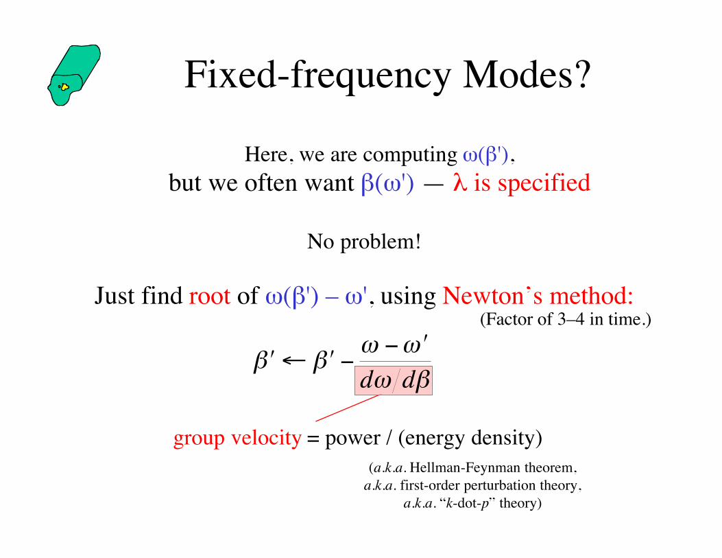
group velocity = power / (energy density)(a.k.a. Hellman-Feynman theorem,
a.k.a. first-order perturbation theory,a.k.a. “k-dot-p” theory)
Fixed-frequency Modes?
Here, we are computing ω(β'),but we often want β(ω') — λ is specified
No problem!
Just find root of ω(β') – ω', using Newton’s method:
′ ← ′ −− ′
β βω ωω βd d
(Factor of 3–4 in time.)
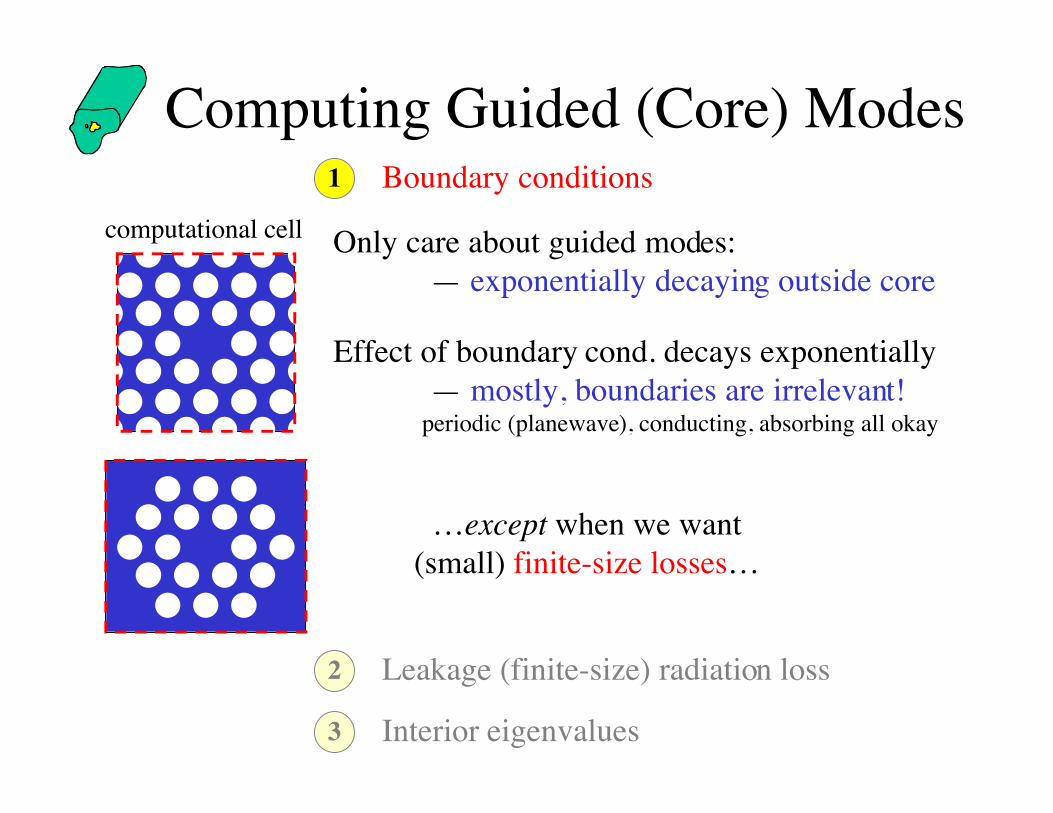
Computing Guided (Core) Modes1 Boundary conditions
2 Leakage (finite-size) radiation loss
3 Interior eigenvalues
Only care about guided modes:— exponentially decaying outside core
computational cell
Effect of boundary cond. decays exponentially— mostly, boundaries are irrelevant!
periodic (planewave), conducting, absorbing all okay
…except when we want(small) finite-size losses…
Computing Guided (Core) Modes1 Boundary conditions
2 Leakage (finite-size) radiation loss
3 Interior eigenvalues
Use PML absorbing boundary layerperfectly matched layer
[ Berenger, J. Comp. Phys. 114, 185 (1994) ]
…with iterative method that works for non-Hermitian (dissipative) systems:
Jacobi-Davidson, …
[ Saitoh, IEEE J. Quantum Elec. 38, 927 (2002) ]
in imaginary z, largest β (fundamental) mode grows exponentially
Or imaginary-distance BPM:
Computing Guided (Core) Modes1 Boundary conditions
2 Leakage (finite-size) radiation loss
3 Interior eigenvalues
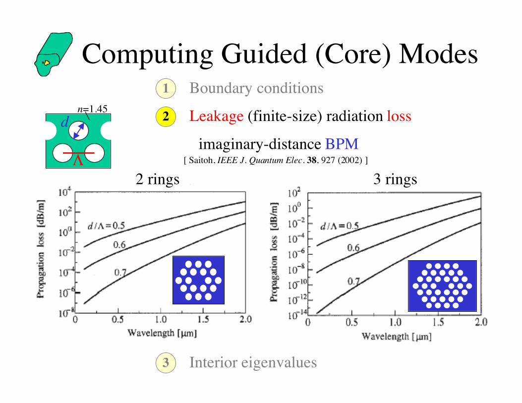
imaginary-distance BPM [ Saitoh, IEEE J. Quantum Elec. 38, 927 (2002) ]
d
Λ
n=1.45
2 rings 3 rings
Computing Guided (Core) Modes1 Boundary conditions
2 Leakage (finite-size) radiation loss
3 Interior eigenvalues
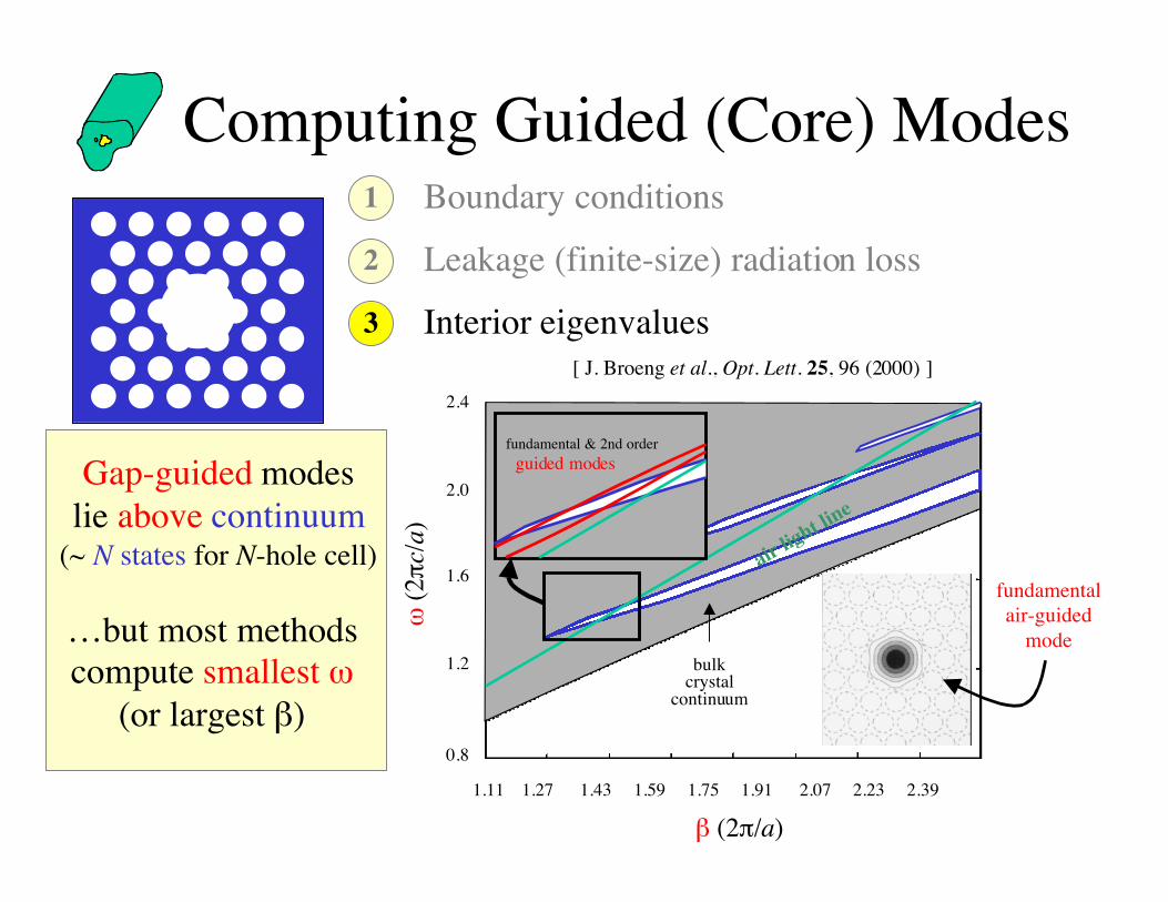
β (2π/a)
[ J. Broeng et al., Opt. Lett. 25, 96 (2000) ]
bulkcrystal
continuum
fundamental & 2nd order guided modes
air light lin
e
fundamentalair-guided
mode
0.8
1.2
1.6
2.0
2.4
1.11 1.27 1.43 1.59 1.75 1.91 2.07 2.23 2.39
ω (
2πc/
a)
Gap-guided modeslie above continuum
(~ N states for N-hole cell)
…but most methodscompute smallest ω
(or largest β)
Computing Guided (Core) Modes1 Boundary conditions
2 Leakage (finite-size) radiation loss
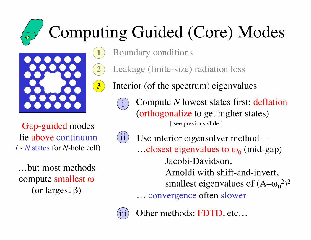
3 Interior (of the spectrum) eigenvalues
Gap-guided modeslie above continuum
(~ N states for N-hole cell)
…but most methodscompute smallest ω
(or largest β)
i Compute N lowest states first: deflation(orthogonalize to get higher states)
[ see previous slide ]
ii Use interior eigensolver method—…closest eigenvalues to ω0 (mid-gap)
Jacobi-Davidson,Arnoldi with shift-and-invert,smallest eigenvalues of (A–ω0
2)2
… convergence often slower
iii Other methods: FDTD, etc…
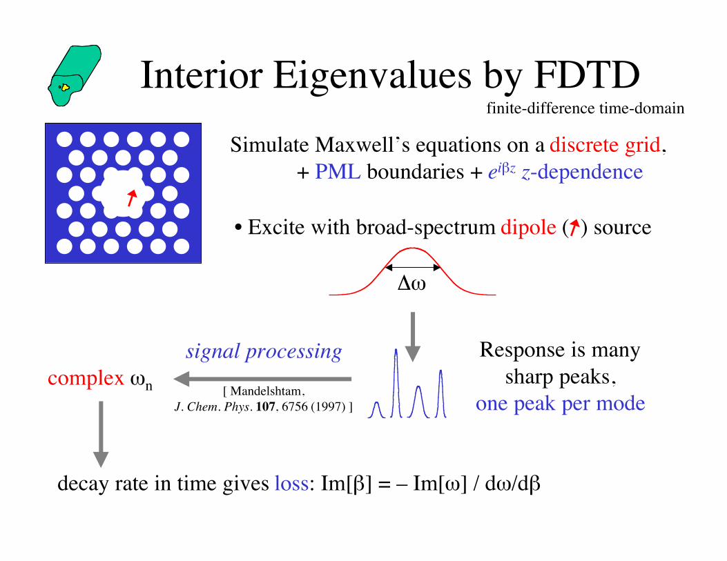
Interior Eigenvalues by FDTDfinite-difference time-domain
Simulate Maxwell’s equations on a discrete grid,+ PML boundaries + eiβz z-dependence
• Excite with broad-spectrum dipole ( ) source
∆ω
Response is manysharp peaks,
one peak per modecomplex ωn [ Mandelshtam,
J. Chem. Phys. 107, 6756 (1997) ]
signal processing
decay rate in time gives loss: Im[β] = – Im[ω] / dω/dβ
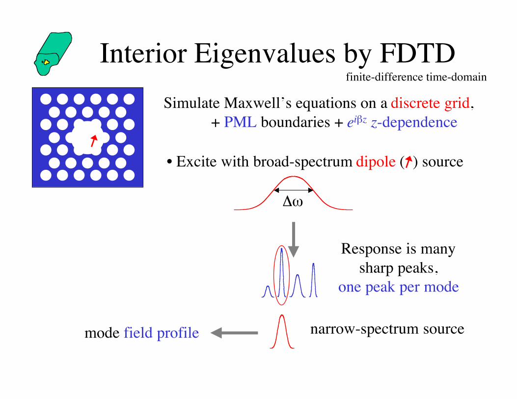
Interior Eigenvalues by FDTDfinite-difference time-domain
Simulate Maxwell’s equations on a discrete grid,+ PML boundaries + eiβz z-dependence
• Excite with broad-spectrum dipole ( ) source
∆ω
Response is manysharp peaks,
one peak per mode
narrow-spectrum sourcemode field profile
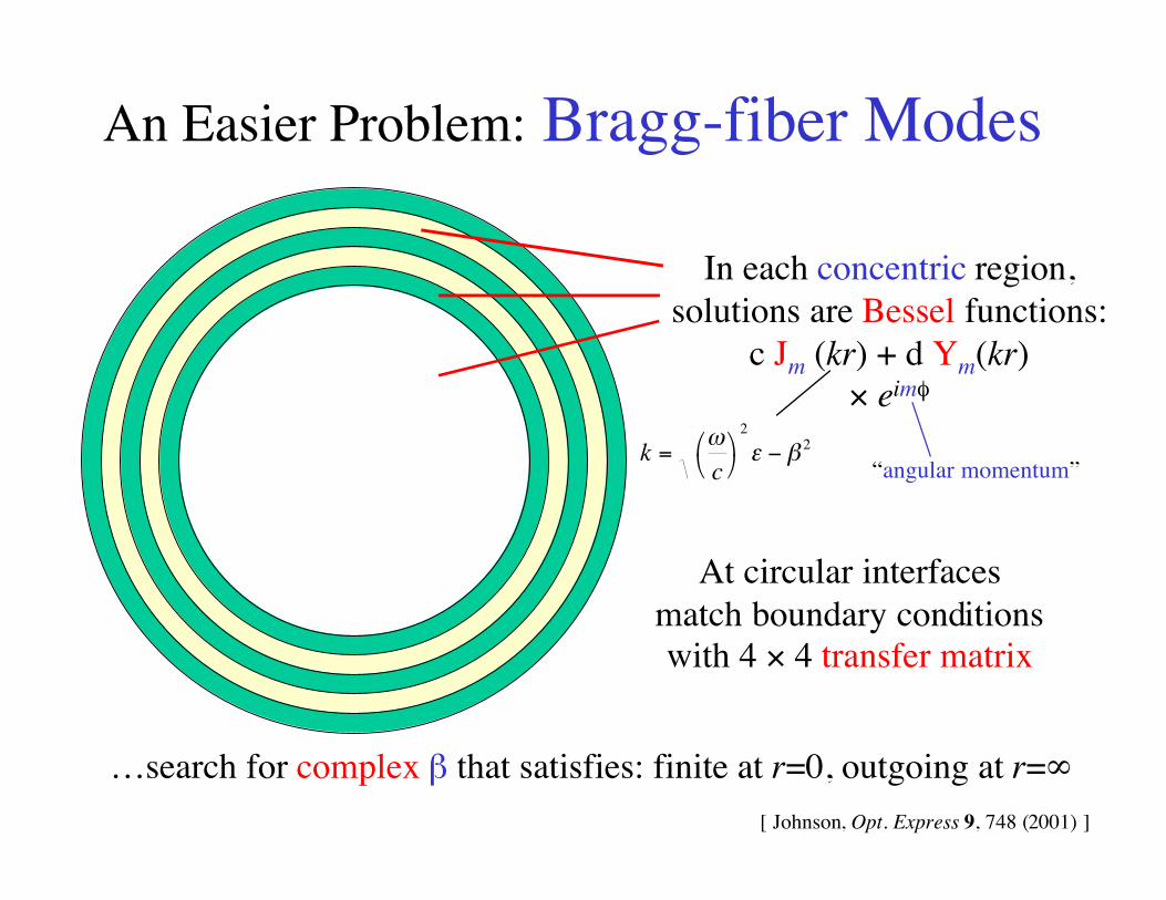
An Easier Problem: Bragg-fiber Modes
In each concentric region,solutions are Bessel functions:
c Jm (kr) + d Ym(kr)× eimφ
“angular momentum”k
c=
−
ωε β
22
At circular interfacesmatch boundary conditionswith 4 × 4 transfer matrix
…search for complex β that satisfies: finite at r=0, outgoing at r=∞
[ Johnson, Opt. Express 9, 748 (2001) ]
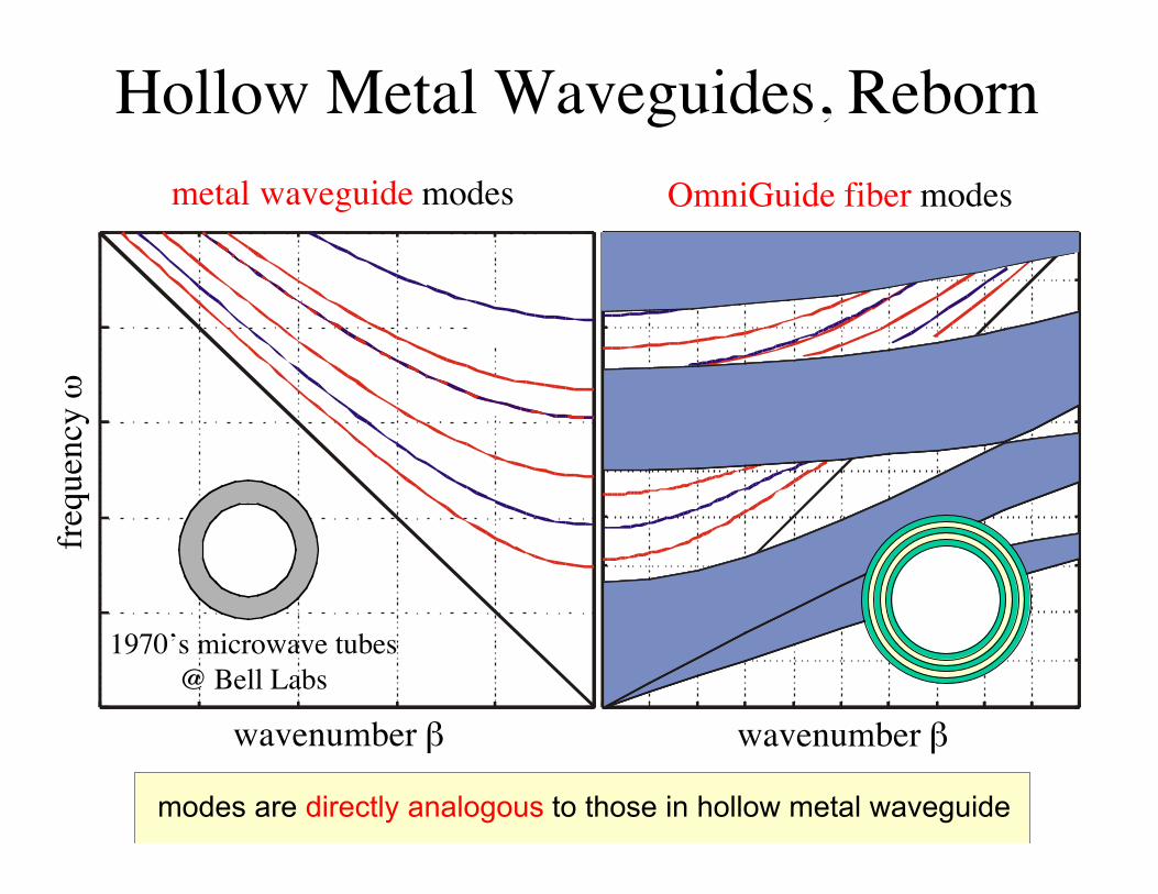
Hollow Metal Waveguides, Reborn
OmniGuide fiber modes
wavenumber βwavenumber β
freq
uenc
y ω
metal waveguide modes
1970’s microwave tubes@ Bell Labs
modes are directly analogous to those in hollow metal waveguide

An Old Friend: the TE01 mode
lowest-loss mode,just as in metal
rE
(near) node at interface= strong confinement
= low losses
non-degenerate mode— cannot be split
= no birefringence or PMD
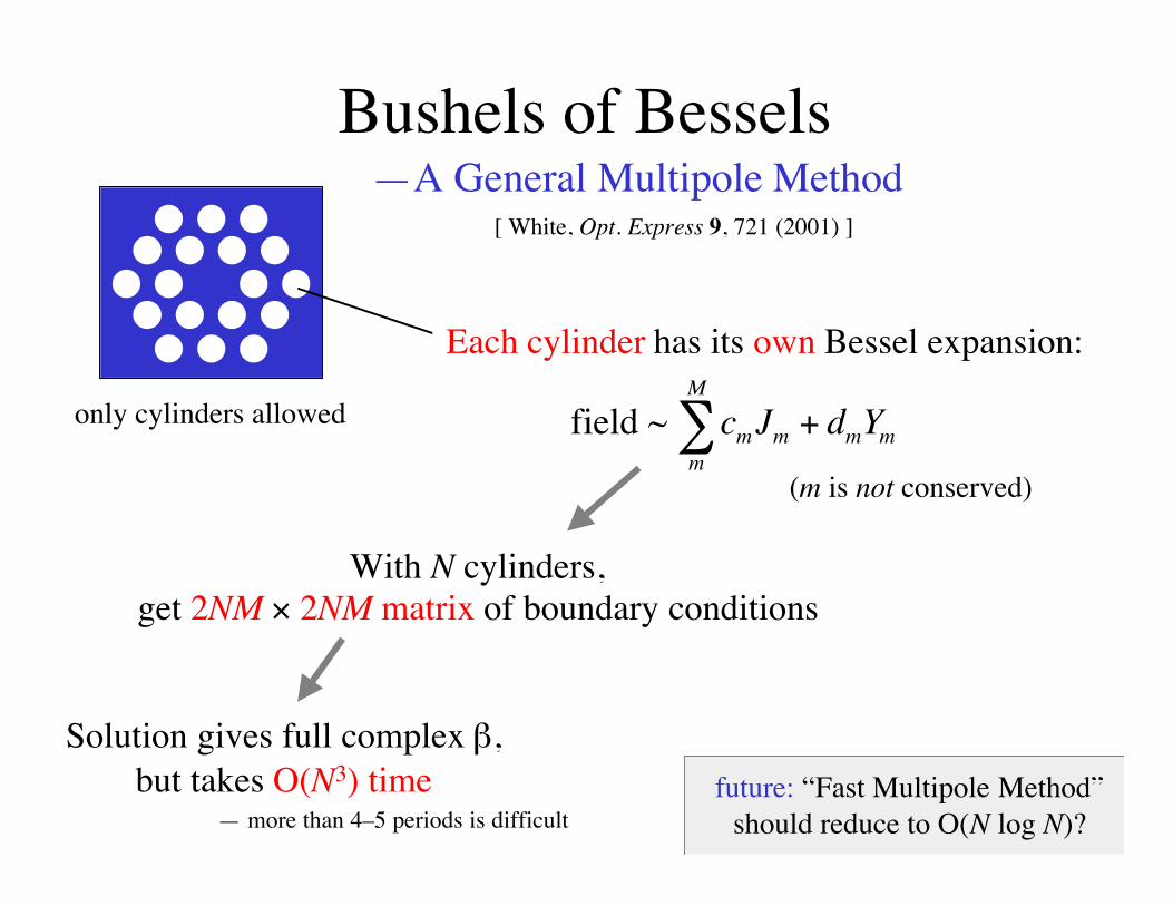
Bushels of Bessels
Each cylinder has its own Bessel expansion:
—A General Multipole Method[ White, Opt. Express 9, 721 (2001) ]
field ~ c J d Ym m m mm
M
+∑(m is not conserved)
With N cylinders,get 2NM × 2NM matrix of boundary conditions
Solution gives full complex β,but takes O(N3) time
— more than 4–5 periods is difficultfuture: “Fast Multipole Method”
should reduce to O(N log N)?
only cylinders allowed
Outline
• What are these fibers (and why should I care)?
• The guiding mechanisms: index-guiding and band gaps
• Finding the guided modes
• Small corrections (with big impacts)
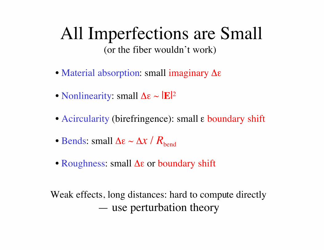
All Imperfections are Small
• Material absorption: small imaginary ∆ε
• Nonlinearity: small ∆ε ~ |E|2
• Acircularity (birefringence): small ε boundary shift
• Bends: small ∆ε ~ ∆x / Rbend
• Roughness: small ∆ε or boundary shift
(or the fiber wouldn’t work)
Weak effects, long distances: hard to compute directly— use perturbation theory
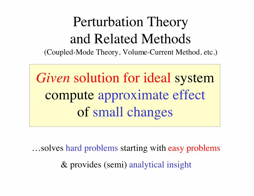
Perturbation Theoryand Related Methods
(Coupled-Mode Theory, Volume-Current Method, etc.)
Given solution for ideal systemcompute approximate effect
of small changes
…solves hard problems starting with easy problems
& provides (semi) analytical insight
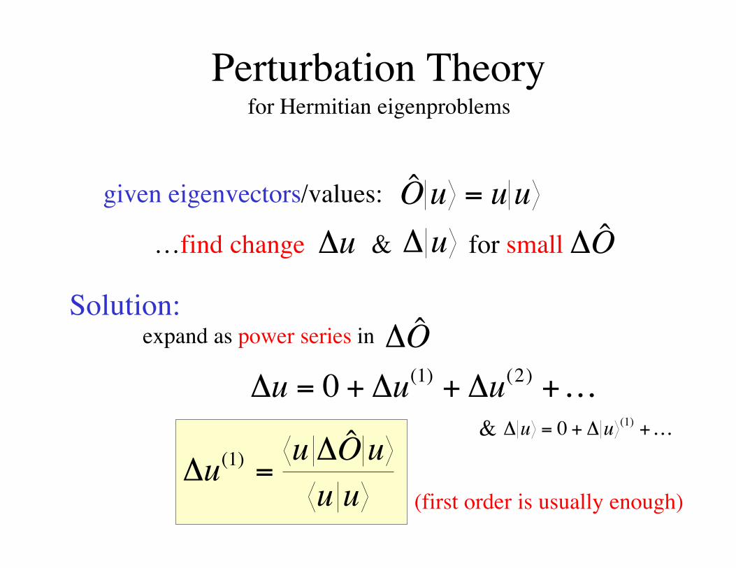
Perturbation Theoryfor Hermitian eigenproblems
given eigenvectors/values: O u u u=
…find change & for small∆u ∆ u ∆O
Solution:expand as power series in ∆O
∆ ∆ ∆u u u= + + +…0 1 2( ) ( )
∆ ∆u u= + +…0 1( )&
∆∆
uu O u
u u( )
ˆ1 =
(first order is usually enough)
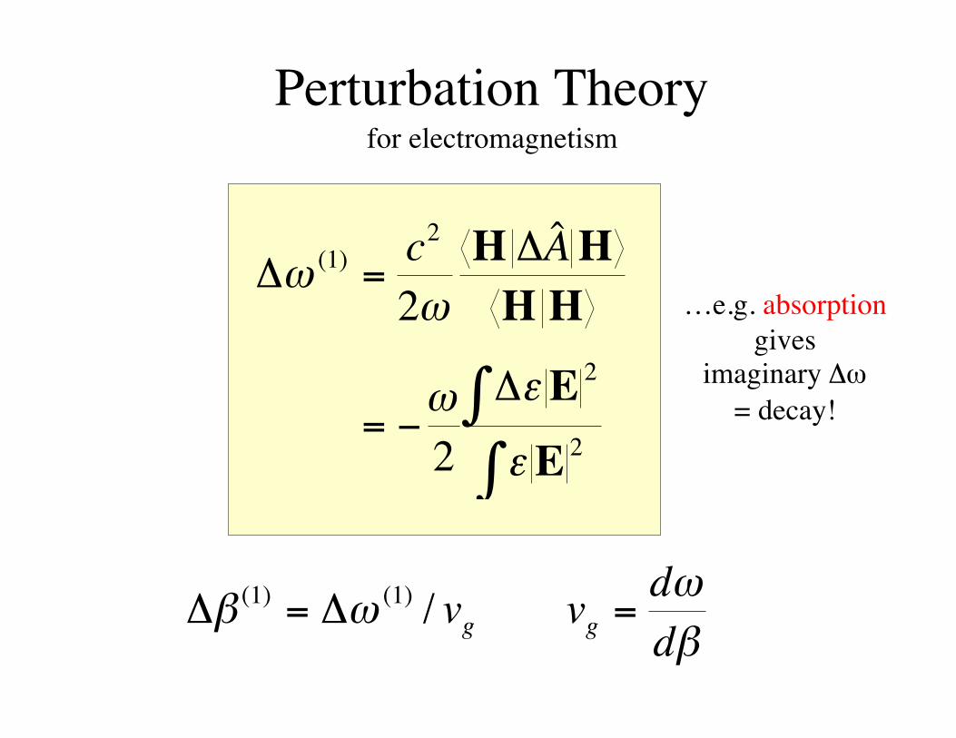
Perturbation Theoryfor electromagnetism
∆∆
∆
ωω
ω ε
ε
( )ˆ
12
2
2
2
2
=
= − ∫∫
c AH HH H
E
E
∆ ∆β ω( ) ( ) /1 1= vg vddg =ωβ
…e.g. absorptiongives
imaginary ∆ω= decay!
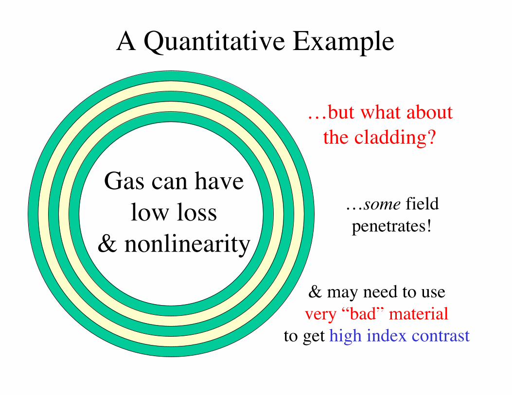
A Quantitative Example
Gas can havelow loss
& nonlinearity
…but what aboutthe cladding?
& may need to usevery “bad” material
to get high index contrast
…some fieldpenetrates!
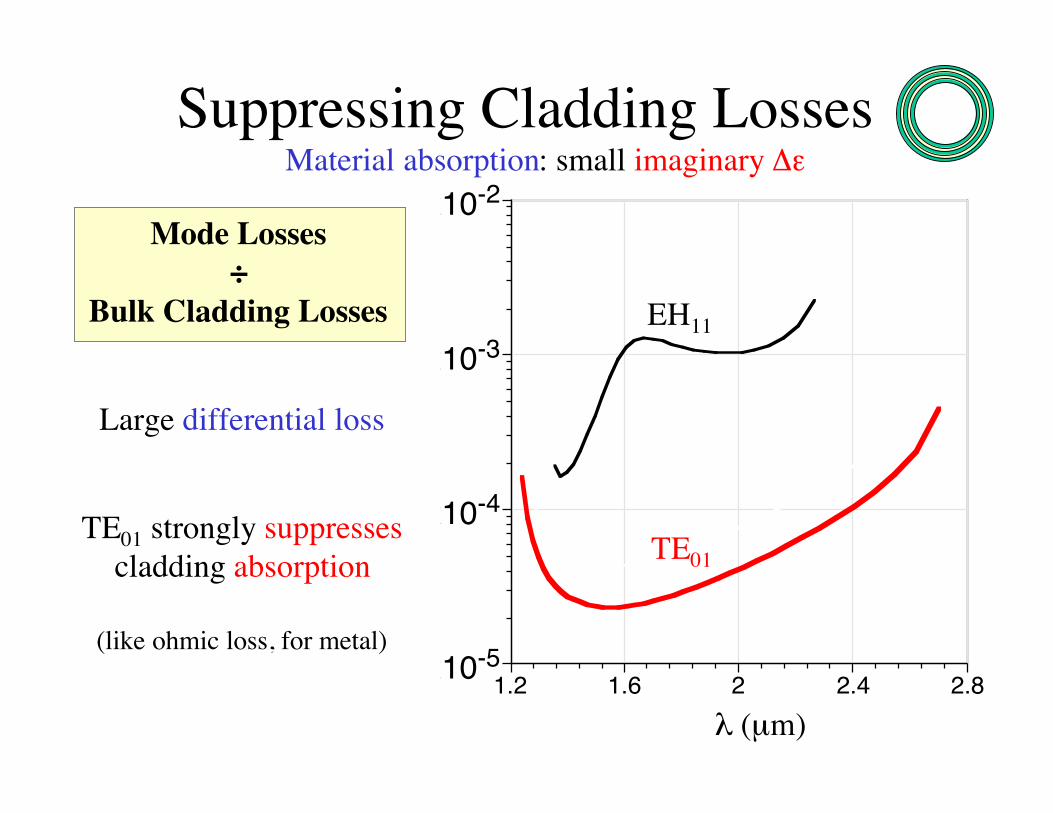
Suppressing Cladding Losses
1x10⁻⁵
1x10⁻⁴
1x10⁻³
1x10⁻²
1.2 1.6 2 2.4 2.8
EH11
TE01
Mode Losses÷
Bulk Cladding Losses
TE01 strongly suppressescladding absorption
(like ohmic loss, for metal)
Large differential loss
λ (µm)
Material absorption: small imaginary ∆ε
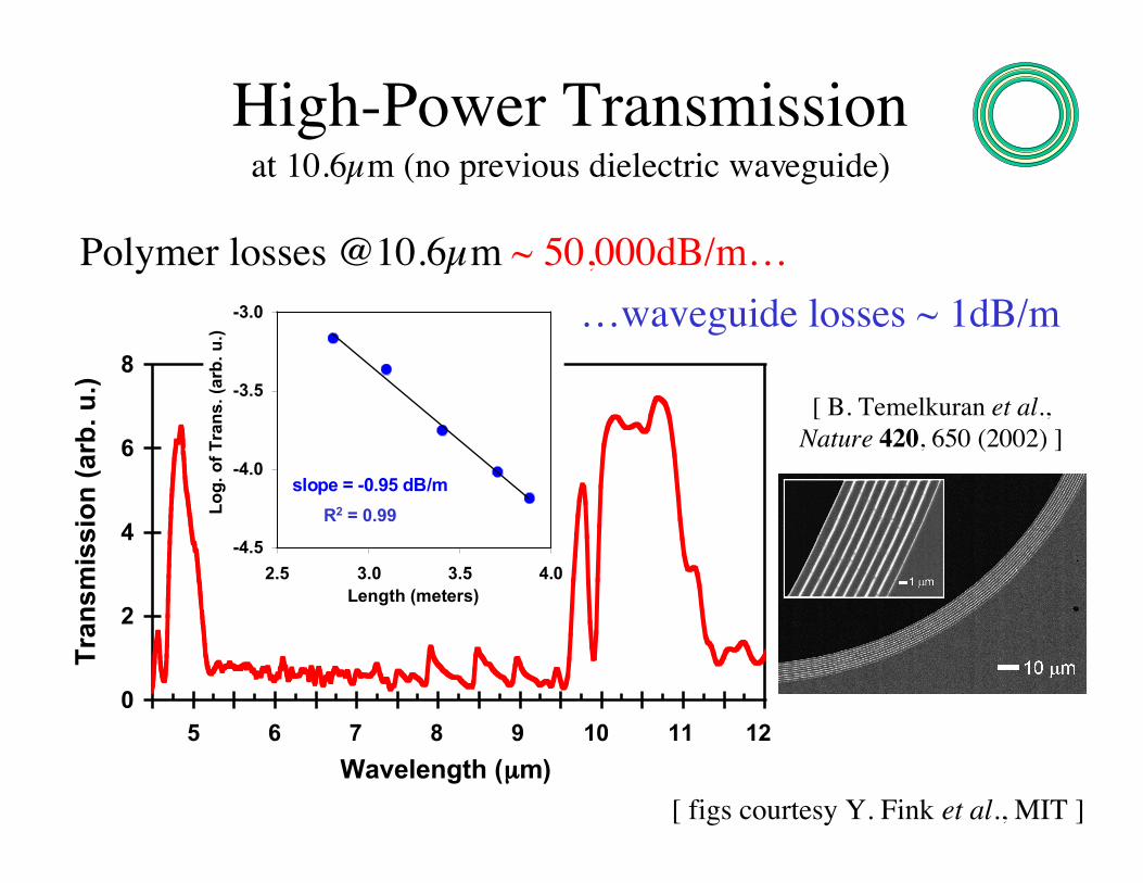
High-Power Transmissionat 10.6µm (no previous dielectric waveguide)
[ figs courtesy Y. Fink et al., MIT ]
0
2
4
6
8
Tra
nsm
issi
on
(ar
b. u
.)
slope = -0.95 dB/m
-4.5
-4.0
-3.5
-3.0
2.5 3.0 3.5 4.0Length (meters)
Lo
g. o
f T
ran
s. (
arb
. u.)
Wavelength (µµµµm)
5 6 7 8 9 1210 11
R2 = 0.99
Polymer losses @10.6µm ~ 50,000dB/m…
…waveguide losses ~ 1dB/m
[ B. Temelkuran et al.,Nature 420, 650 (2002) ]
Quantifying Nonlinearity
∆β ~ power P ~ 1 / lengthscale for nonlinear effects
γ = ∆β / P
= nonlinear-strength parameter determiningself-phase modulation (SPM), four-wave mixing (FWM), …
(unlike “effective area,”tells where the field is,
not just how big)
Kerr nonlinearity: small ∆ε ~ |E|2
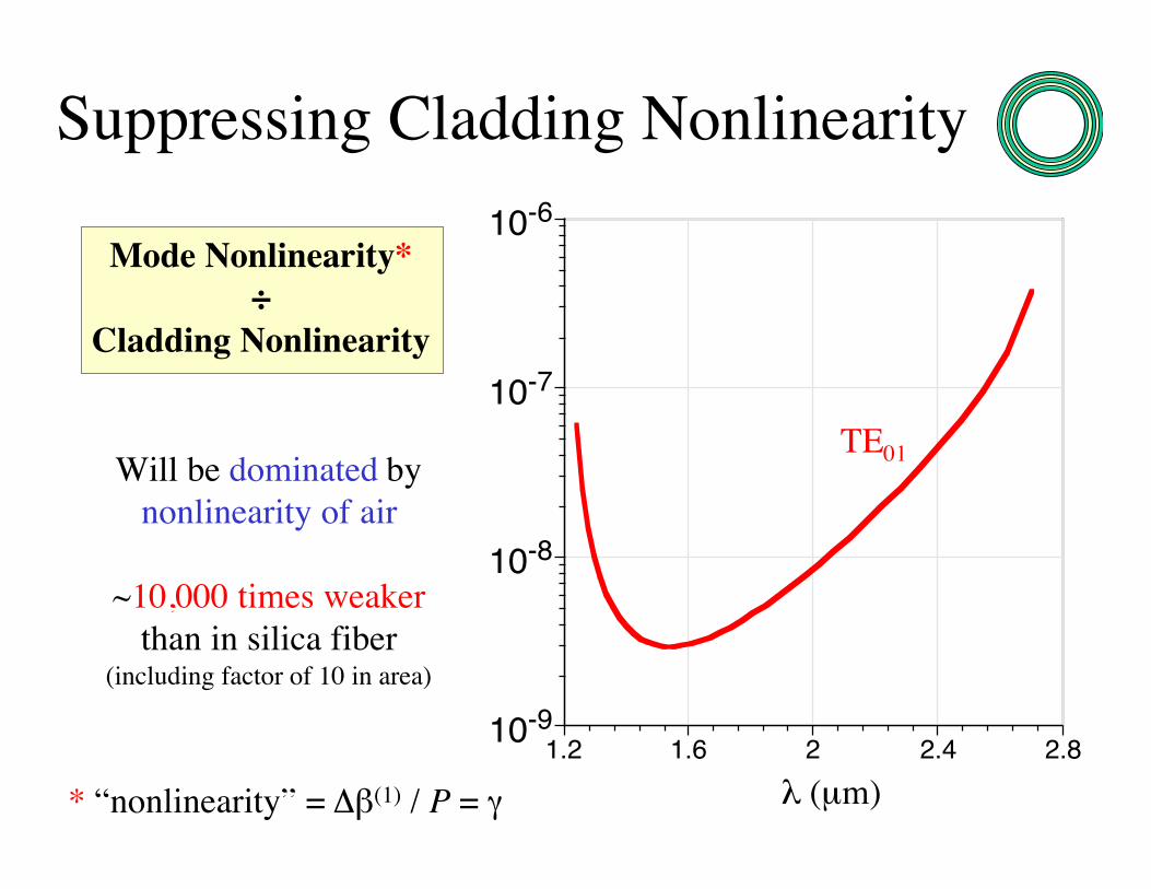
1x10⁻⁹
1x10⁻⁸
1x10⁻⁷
1x10⁻⁶
1.2 1.6 2 2.4 2.8
Suppressing Cladding Nonlinearity
TE01
Mode Nonlinearity*÷
Cladding Nonlinearity
λ (µm)
Will be dominated bynonlinearity of air
~10,000 times weakerthan in silica fiber
(including factor of 10 in area)
* “nonlinearity” = ∆β(1) / P = γ

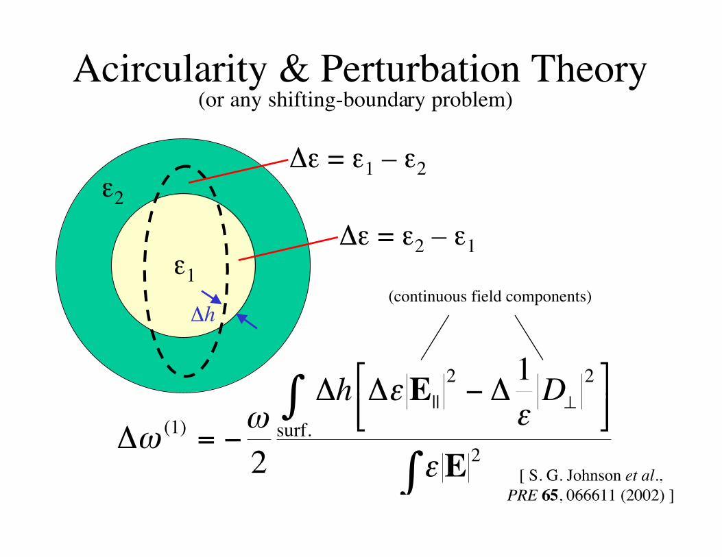
Acircularity & Perturbation Theory
ε1
ε2
∆ε = ε1 – ε2
∆ε = ε2 – ε1
… just plug ∆ε’s intoperturbation formulas?
FAILS for high index contrast!
beware field discontinuity…fortunately, a simple correction exists [ S. G. Johnson et al.,
PRE 65, 066611 (2002) ]
(or any shifting-boundary problem)
Acircularity & Perturbation Theory
ε1
ε2
∆ε = ε1 – ε2
∆ε = ε2 – ε1
[ S. G. Johnson et al.,PRE 65, 066611 (2002) ]
(or any shifting-boundary problem)
∆
∆ ∆ ∆
ωω
εε
ε( )
||1
2 2
22
1
= −
−
⊥∫
∫
h DE
Esurf.
∆h(continuous field components)

Loss from Roughness/Disorder
imperfection acts like a volume currentr rJ E~ ∆ε 0
volume-current methodor Green’s functions with first Born approximation
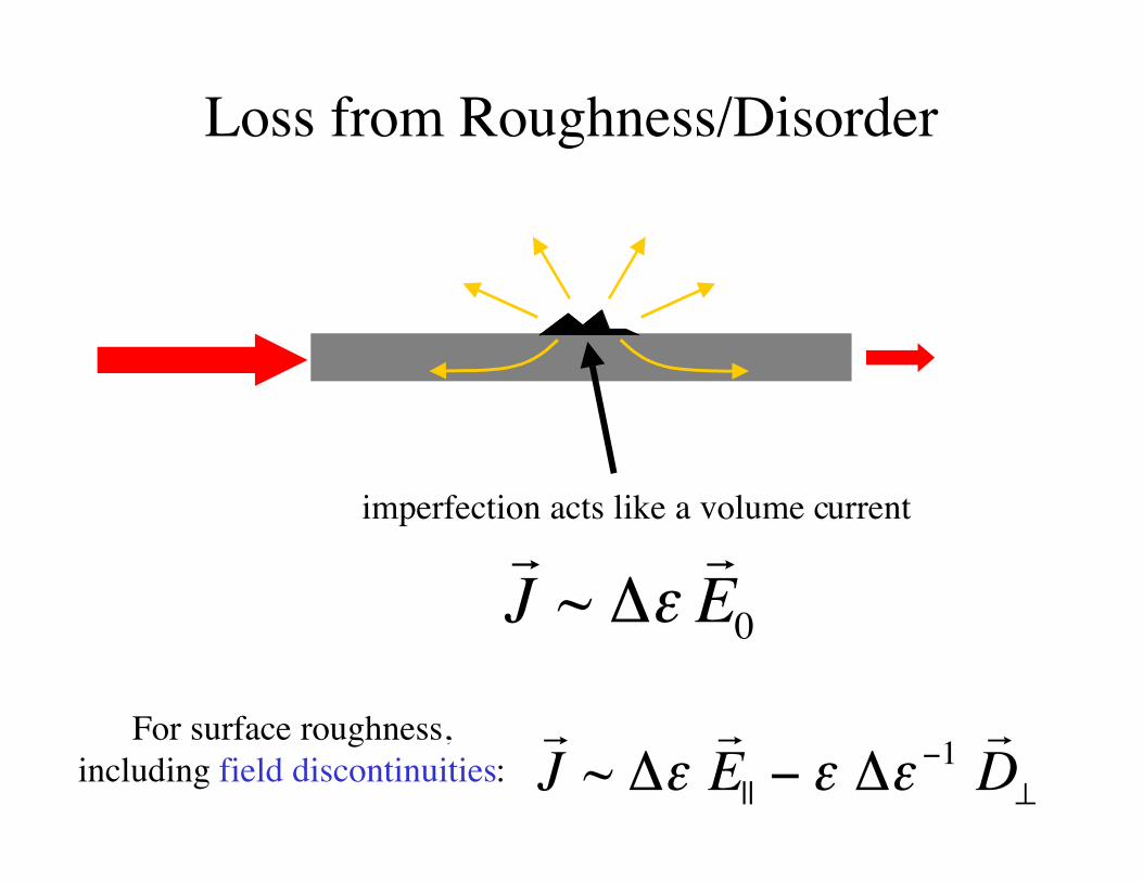
Loss from Roughness/Disorder
imperfection acts like a volume currentr rJ E~ ∆ε 0
r r rJ E D~ ||∆ ∆ε ε ε− −
⊥1
For surface roughness,including field discontinuities:
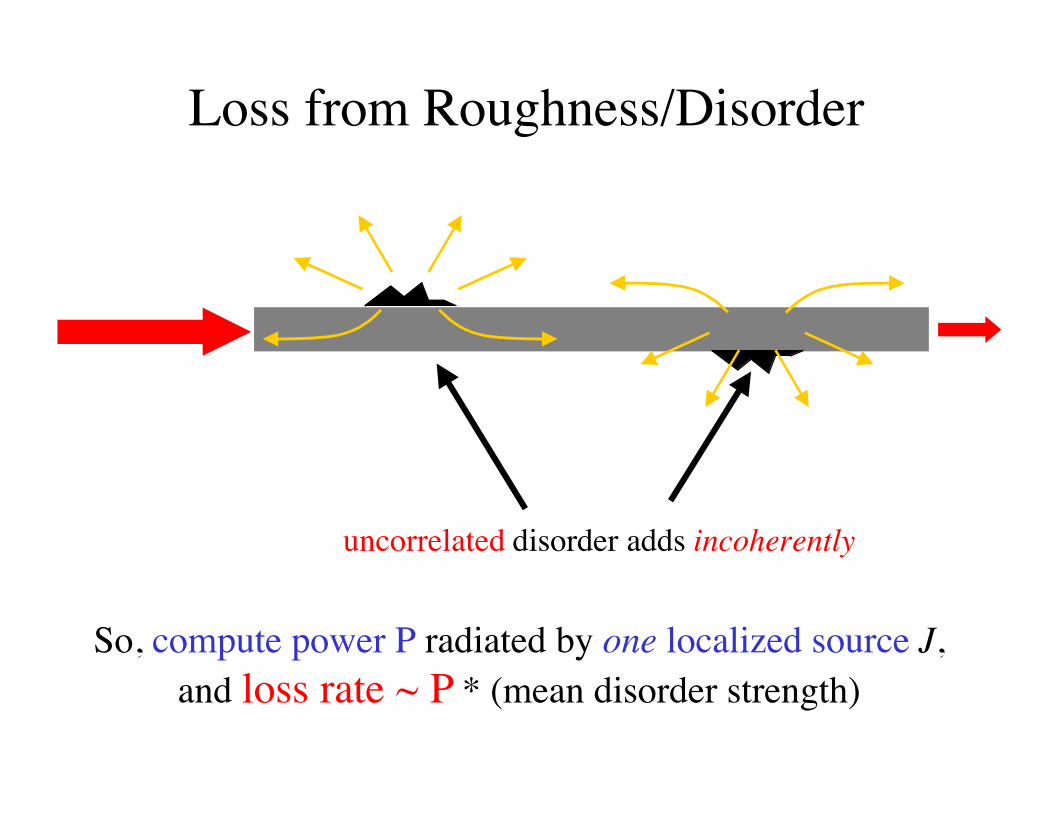
Loss from Roughness/Disorder
uncorrelated disorder adds incoherently
So, compute power P radiated by one localized source J,and loss rate ~ P * (mean disorder strength)
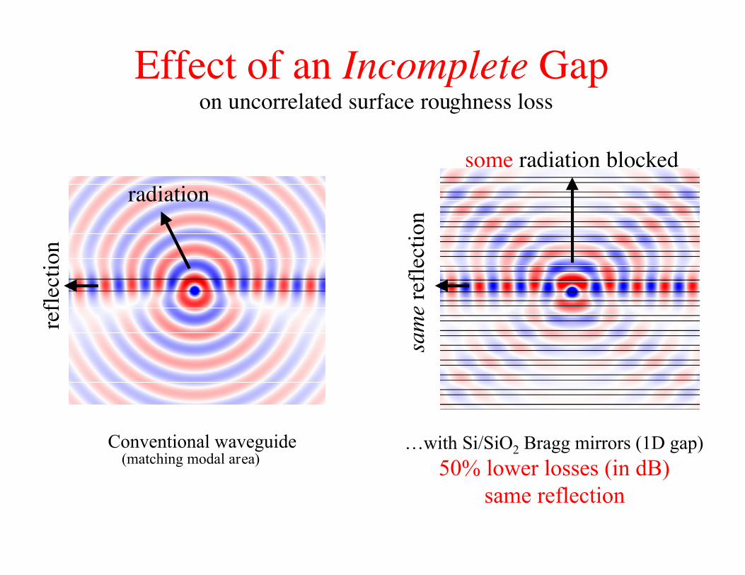
Conventional waveguide
radiation
refl
ecti
onEffect of an Incomplete Gap
…with Si/SiO2 Bragg mirrors (1D gap)50% lower losses (in dB)
same reflection
some radiation blocked
sam
e re
flec
tion
(matching modal area)
on uncorrelated surface roughness loss
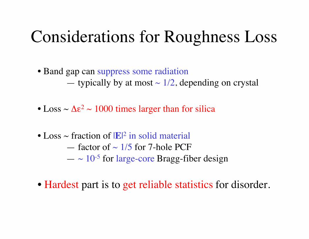
Considerations for Roughness Loss
• Band gap can suppress some radiation— typically by at most ~ 1/2, depending on crystal
• Loss ~ ∆ε2 ~ 1000 times larger than for silica
• Loss ~ fraction of |E|2 in solid material— factor of ~ 1/5 for 7-hole PCF— ~ 10-5 for large-core Bragg-fiber design
• Hardest part is to get reliable statistics for disorder.
Using perturbations to designbig effects
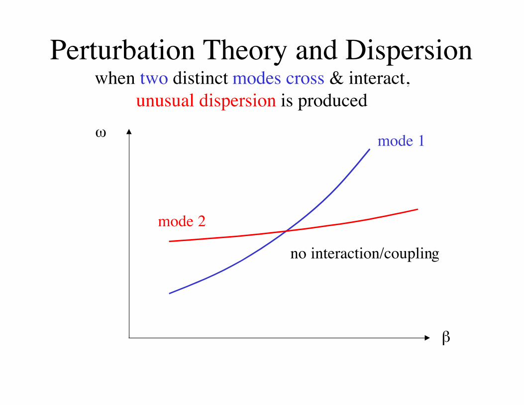
Perturbation Theory and Dispersion
ω
β
when two distinct modes cross & interact,unusual dispersion is produced
no interaction/coupling
mode 1
mode 2
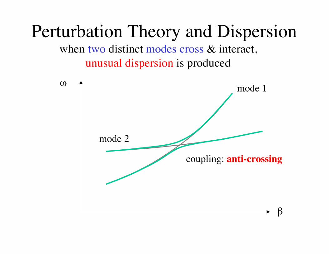
Perturbation Theory and Dispersion
ω
β
when two distinct modes cross & interact,unusual dispersion is produced
coupling: anti-crossing
mode 1
mode 2
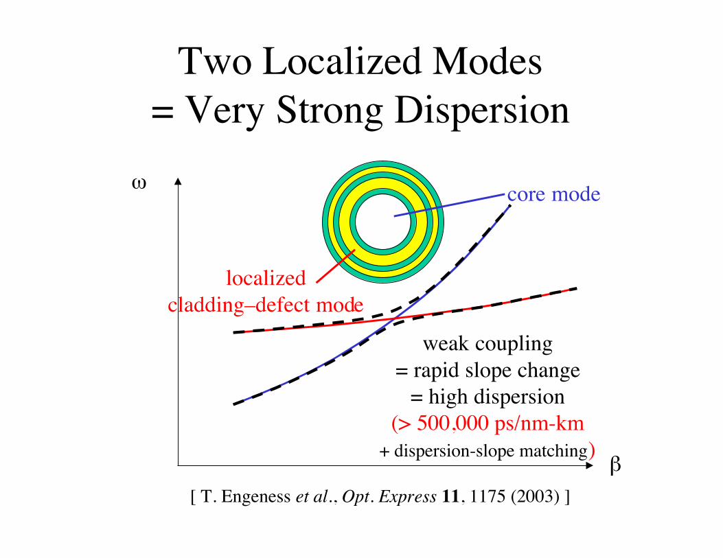
Two Localized Modes= Very Strong Dispersion
ω
β
core mode
localizedcladding–defect mode
weak coupling= rapid slope change
= high dispersion(> 500,000 ps/nm-km
+ dispersion-slope matching)
[ T. Engeness et al., Opt. Express 11, 1175 (2003) ]
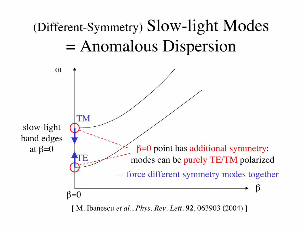
(Different-Symmetry) Slow-light Modes= Anomalous Dispersion
ω
β
[ M. Ibanescu et al., Phys. Rev. Lett. 92, 063903 (2004) ]
β=0
slow-lightband edges
at β=0 β=0 point has additional symmetry:modes can be purely TE/TM polarized
TM
TE
— force different symmetry modes together
(Different-Symmetry) Slow-light Modes= Anomalous Dispersion
[ M. Ibanescu et al., Phys. Rev. Lett. 92, 063903 (2004) ]
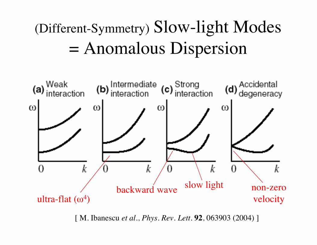
ultra-flat (ω4)backward wave slow light non-zero
velocity
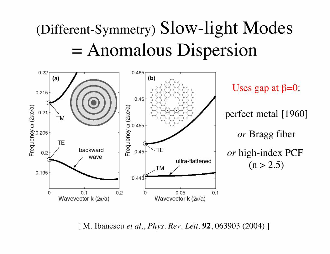
(Different-Symmetry) Slow-light Modes= Anomalous Dispersion
[ M. Ibanescu et al., Phys. Rev. Lett. 92, 063903 (2004) ]
Uses gap at β=0:
perfect metal [1960]
or Bragg fiber
or high-index PCF (n > 2.5)
Further Reading
Reviews:
• J. D. Joannopoulos, R. D. Meade, and J. N. Winn, Photonic Crystals:Molding the Flow of Light (Princeton Univ. Press, 1995).
• P. Russell, “Photonic-crystal fibers,” Science 299, 358 (2003).
This Presentation, Free Software, Other Material:
http://ab-initio.mit.edu/photons/tutorial