microeconomics i and statistics
TRANSCRIPT

As per new B Com CBCS syllabus 2017 for CU
Microeconomics I and Statistics
SECOND EDITION
Professor, Department of EconomicsUniversity of Calcutta
Associate Professor, Department of EconomicsHooghly Women’s College
University of Burdwan
Panchanan Das
Anindita Sengupta
Microeconomics.indb 1 6/21/2017 6:43:19 PM
© Oxford University Press. All rights reserved.
Oxford
Universi
ty Pre
ss

3Oxford University Press is a department of the University of Oxford.
It furthers the University’s objective of excellence in research, scholarship, and education by publishing worldwide. Oxford is a registered trademark of
Oxford University Press in the UK and in certain other countries.
Published in India by Oxford University Press
Ground Floor, 2/11, Ansari Road, Daryaganj, New Delhi 110002, India
© Oxford University Press 2015, 2017
The moral rights of the author/s have been asserted.
First Edition published in 2015Second Edition published in 2017
All rights reserved. No part of this publication may be reproduced, stored in a retrieval system, or transmitted, in any form or by any means, without the
prior permission in writing of Oxford University Press, or as expressly permitted by law, by licence, or under terms agreed with the appropriate reprographics
rights organization. Enquiries concerning reproduction outside the scope of the above should be sent to the Rights Department, Oxford University Press, at the
address above.
You must not circulate this work in any other form and you must impose this same condition on any acquirer.
ISBN-13: 978-0-19-948173-6ISBN-10: 0-19-948173-3
Typeset in GaramondPremrProby Ideal Publishing Solutions, Delhi
Printed in India by Magic International (P) Ltd., Greater Noida
Cover image: pedrosek / Shutterstock
Third-party website addresses mentioned in this book are providedby Oxford University Press in good faith and for information only.
Oxford University Press disclaims any responsibility for the material contained therein.
Economics_FM.indd 2 6/22/2017 1:52:55 PM
© Oxford University Press. All rights reserved.
Oxford
Universi
ty Pre
ss
PrefaceThis text on Microeconomics I and Statistics is strictly for Paper GE 1.1 Chg. of Semester I which is common to honours and general courses in the new syllabus prescribed by the University of Calcutta under the framework of choice based credit system (CBCS) of the University Grants Commission (UGC). The book is designed to cover all the topics keeping in mind the structure of CBCS provided in the UGC guidelines of CBCS. As the total credit hours for each paper under the new system are strictly specified, the chapters in the book are precise, yet comprehensive and easy-to-understand for honours and general undergraduate students of commerce under the University of Calcutta. While it contains the necessary topics completely covering the syllabus of the University of Calcutta, it also captures well the syllabi prescribed by the leading universities in India.
About the Book Microeconomics I and Statistics is designed for undergraduate commerce students and others in learning microeconomic theory and basic statistics. The main purpose is to articulate the basic questions of microeconomic theory and statistical problems in a student-friendly manner. The primary objective is to motivate the students to learn the concepts, to conceptualize the problem properly, and to secure good marks in the University examination. Some problems on microeconomics are discussed with mathematical treatment along with graphical illustration to understand the problem clearly and more logically. The mathematical parts are for advanced learning, especially for curious students, while others could skip these parts without losing the logic of the problem.
Key Features • The contents of the book and sequence of topics are prepared by following theCBCS-based new
syllabus prescribed by the University of Calcutta.• Practicalexamplesareinsertedtomaketheorieseasilyunderstandabletothestudents.• Numericalproblemsareprovidedtounderstanddifferentaspectsofmicroeconomicsandstatistics.• Aplethoraofnumericalexamples,andexercisesincludingmultiple-choicequestionswithanswersare
provided by following the probable question patterns in the semester system.• Solutions of theUniversity questions aswell asmodel questions are provided,whichwill help the
students to prepare for their examinations.
Organization of the Book The first part containing microeconomic theory is divided into five chapters by following the sequence as shown in Module I of the syllabus.
Chapter 1 provides a basic idea of the demand function and the related issues on law of demand. The law of demand is explained and illustrated in terms of charts and diagrams. The perceptions of elasticities of demand have been discussed clearly. Ideas about the elasticities of demand are necessary to conceptualize
Microeconomics.indb 4 6/21/2017 6:43:20 PM
© Oxford University Press. All rights reserved.
Oxford
Universi
ty Pre
ss

Preface v
thenatureofdemandfordifferentcommodities.Thischaptertakescareofdifferentconceptsofelasticitiesof demand in a comprehensive manner.
Chapter 2 focuses on the problems of consumers’ behaviour under the framework of Marshallian cardinal utility approach, and ordinal utility approach developed first by Hicks and Allen. In a market-based economy, consumers determine the demand for goods and services, and the supply of inputs used in production by solvingtheconstrainedutilitymaximizationproblem.Theconceptsofpriceeffect,substitutioneffect,andincomeeffectareillustratedgraphicallytoeasilyunderstandthedifferentshapesofthedemandcurvefora commodity.
Chapter 3 discusses the concepts of production function, both under short run and long run. Production is an economic activity performed by the firms. Firms determine the supply of output and demand for inputs by solving either constrained output maximization, or constrained cost minimization, or ultimately, profit maximization problem. The problems of constrained optimization that a rational firm has to face is analysed in this chapter with the help of isoquants and isocost lines. The notion of homogeneous function is highly mathematical. However, we have used this concept in a simple form to analyse the behaviour of the long-run production function.
Chapter 4containsdifferentideasaboutcostsofproductionmostlyrelevantinbusinesseconomics.Costfunctionsarebasicallythemirrorimageofproductionfunctions.Thederivationofdifferentaspectsof cost function from the production function has been illustrated intelligibly by using simple functional form as well as graphical techniques.
Chapter 5 deals with the market analysis. Exchange between consumers and firms—the two basic economic agents—takes place in the market to determine equilibrium quantity and price of a commodity. Microeconomics deals with the market for a particular commodity. This chapter deals with the nature and characteristics of a perfectly competitive market. Walrasian and Marshallian stability in a competitive market are illustrated lucidly. The impacts of taxes and subsidy in the framework of demand and supply are also discussed in this chapter.
The second part of this book deals with statistics based on Module II of the syllabus prescribed by the University of Calcutta. All chapters in this module contain sufficient numerical examples and many numerical problems for self-assessment of the students.
Chapter 1 of the second part of this book discusses some fundamentals in statistics. It covers the basic steps to be followed in the collection of data and their proper presentation in tabular form, graphs, and figures. Summarization of data is an important step for statistical analysis. Frequency distribution is a popular formofsummarizationofdata.Thischapterillustratesthedifferentaspectsoffrequencydistributionandits diagrammatic presentation.
Chapter 2 covers the measures of central tendency and discusses how to calculate them, and under what conditions a particular measure may be used most appropriately. The mean, median, and mode are the popular measures of central tendency. This chapter deals with these measures of central tendency of a distribution.
Chapter 3 deals with the measures of dispersion that seek to quantify the variability of the data. This chapter is concerned with some important measures of dispersion such as range, quartile deviation, mean deviation,andstandarddeviation,toquantifytheextenttowhichthevaluesinadistributiondifferfromthe average of the distribution.
Chapter 4 takes care of various statistical techniques to distinguish among the various shapes of a distribution. This chapter makes the student familiar with some statistical measures in terms of moments, the concept of skewness and kurtosis.
Microeconomics.indb 5 6/21/2017 6:43:20 PM
© Oxford University Press. All rights reserved.
Oxford
Universi
ty Pre
ss

vi Preface
Chapter 5containsdifferentmethodsofinterpolationusedinstatisticsandmathematics.Interpolation,is not only useful in statistics, but is also useful in science, business, or any time there is a need to predict values that fall within two existing data points.
Acknowledgements It is a great pleasure to thank those people who have helped us put this book together. Their generosity and insights were generous. We, of course, are solely responsible for any errors. We acknowledge our debts especially to our colleagues and friends at the University of Calcutta, Goenka College of Commerce and Business Administration, and Hooghly Women’s College, many of whom have been of immense help while preparing this text.
We like to thank the Head of the Department of Economics of the University of Calcutta, and the PrincipalofHooghlyWomen’sCollegewhoinspiredusatdifferentstagesoftheproject.Commentsgivenat the early stage by several colleagues after going through large portions of the manuscript very much improved the book.
We are grateful to all that we have discovered while teaching our students. We hope this book can serve to help them. Comments made by the reviewers are gratefully acknowledged. We also thank the editorial team at Oxford University Press, India for all their patience and support.
Panchanan DasAnindita Sengupta
Microeconomics.indb 6 6/21/2017 6:43:20 PM
© Oxford University Press. All rights reserved.
Oxford
Universi
ty Pre
ss

Brief ContentsPreface ivDetailed Contents viiiFeatures of the Book xiiRoad Map xiv
PART I MICROECONOMICS I 1
1. Basics of Demand 3
2. Theory of Consumer Behaviour 27
3. Theory of Production 58
4. Theory of Cost 92
5. Perfect Competition 113
Question Bank 135Solved CU Question Papers—2014–2016 140Model Question Papers 166
PART II STATISTICS 171
1. Fundamentals 173
2. Measures of Central Tendency 210
3. Measures of Dispersion 239
4. Moments, Skewness, and Kurtosis 257
5. Interpolation 271
Question Bank 286Solved CU Question Papers—2014–2016 294Model Question Papers 323About the Authors 330
Microeconomics.indb 7 6/21/2017 6:43:20 PM
© Oxford University Press. All rights reserved.
Oxford
Universi
ty Pre
ss

Detailed ContentsPreface ivBrief Contents viiFeatures of the Book xiiRoad Map xiv
PART I MICROECONOMICS I 1
1. Basics of Demand 3 1.1 Introduction 3
1.2 Demand Function 31.3 The Law of Demand 5
1.3.1 Demand Schedule 61.3.2 Derivation of Individual
Demand Curve 61.3.3 Derivation of Market Demand
Curve 61.3.4 Movement along the Demand
Curve 71.3.5 Shifting of the Demand
Curve 81.4 Exceptions to the Law of Demand 9
1.4.1 Giffen Goods 91.4.2 Conspicuous Consumption 91.4.3 Conspicuous Necessities 10
1.4.4 Ignorance 10 1.4.5 Emergencies 10
1.4.6 Future Changes in Prices 111.4.7 Change in Fashion 11
1.5 Elasticity of Demand 111.5.1 Own Price Elasticity of
Demand 111.5.2 Measurement of Own Price
Elasticity of Demand 121.5.3 Elastic and Inelastic
Demand 151.5.4 Distinction between Slope of a
Demand Curve and Elasticity of Demand 16
1.5.5 Cross-price Elasticity of Demand 18
1.5.6 Income Elasticity of Demand 19
1.5.7 Measurement of Income Elasticity of Demand 20
2. Theory of Consumer Behaviour 27 2.1 Introduction 27
2.2 Marshallian Utility Theory 282.2.1 Basic Assumptions of Cardinal
Utility Theory 282.2.2 Equilibrium of the Consumer in
the Cardinal Utility Theory 302.2.3 Derivation of the Demand
Curve from the Cardinal Utility Theory 33
2.2.4 Consumer’s Surplus in the Cardinal Utility Theory 34
2.2.5 Limitations of Cardinal Utility Theory 35
2.3 OrdinalUtilityTheoryorIndifferenceCurve Theory 36
2.3.1 Axioms of Choice in the Ordinal Utility Theory 36
2.3.2 Indifference Curve and Indifference Map 38
2.3.3 Properties of Indifference Curve 39
2.4 Budget Line 432.5 Consumer’s Equilibrium 442.6 Income–Consumption Curve 462.7 Price–Consumption Curve 48
2.7.1 Derivation of Demand Curve from Price–Consumption Curve 48
Microeconomics.indb 8 6/21/2017 6:43:20 PM
© Oxford University Press. All rights reserved.
Oxford
Universi
ty Pre
ss
Detailed Contents ix
2.8 Hicksian Decomposition of Price EffectintoSubstitutionEffectandIncomeEffect 49
2.8.1 Substitution Effect and Income Effect for Normal, Inferior, and Giffen Goods 50
2.9 DemandCurveforNormal,Inferior,andGiffenGoods 51
2.10 IndifferenceCurveTheoryisBetterthan Marshallian Cardinal Utility Theory—Reasons 52
3. Theory of Production 58 3.1 Introduction 58
3.2 Concept of Production 583.3 Factors of Production 593.4 Production Function 593.5 Total Product, Average Product,
and Marginal Product 603.6 Short-run Production: Laws of
Variable Proportions 613.7 Relation between Total Product
and Average Product 633.8 Relation between Total Product
and Marginal Product 643.9 Relation between Average
Product and Marginal Product 65 3.10 Stages of Production 66 3.11 Short-run Equilibrium of a Firm 67 3.12 Long-run Production 68
3.12.1 Isoquant 68 3.12.2 Slope of an Isoquant:
Marginal Rate of Technical Substitution 69
3.12.3 Properties of Isoquant 71 3.13 Ridge Lines and Economic Region
of Production 74 3.14 Isocost Line 75 3.15 Optimal Input Combination 78
3.15.1 Output Maximization Subject to Cost Constraint 78
3.15.2 Cost Minimization Subject to Output Constraint 81
3.16 Expansion Path 83 3.17 Returns to Scale 85
3.18 Homogeneous Production Function and Returns to Scale 87
4. Theory of Cost 92 4.1 Introduction 92
4.2 Accounting Cost and Economic Cost 93
4.3 Private Cost and Social Cost 944.4 Fixed Cost and Variable Cost 944.5 Short-run Cost and Long-run Cost 974.6 Short-run Total Cost Curve,
Short-run Total Fixed Cost Curve, and Short-run Total Variable Cost Curve 98
4.7 Short-run Average Cost Curve, Short-run Average Fixed Cost Curve, and Short-run Average Variable Cost Curve 99
4.7.1 Derivation of Short-run Average Fixed Cost Curve 99
4.7.2 Derivation of Short-run Average Variable Cost Curve 100
4.7.3 Derivation of Short-run Average Cost Curve 101
4.8 Marginal Cost 1024.8.1 Short-run Marginal Cost
Curve 102 4.8.2. Relation between Short-run
Average Cost and Short-run Marginal Cost 103
4.9 Long-run Total Cost Curve 104 4.11 Long-run Average Cost Curve 106 4.11 Long-run Marginal Cost Curve 109
5. Perfect Competition 113 5.1 Introduction 113
5.2 Meaning of Market in Economics 1135.3 Features of Perfectly Competitive
Market 1155.4 Concept of Revenue 1165.5 Short-run Equilibrium of the Firm
in a Perfectly Competitive Market 1185.6 Short-run Supply Curve of the
Firm and the Industry 121
Microeconomics.indb 9 6/21/2017 6:43:20 PM
© Oxford University Press. All rights reserved.
Oxford
Universi
ty Pre
ss
x Detailed Contents
5.7 Long-run Equilibrium of the Firm and the Industry 124
5.8 Producer Surplus under Perfect Competition 126
5.9 Stability Analysis—Walrasian and Marshallian 127
5.10 Demand–Supply Analysis: Impact of Taxes and Subsidy 130
Question Bank 135Solved CU Question Papers—2014–2016 135Model Question Papers 161
PART II STATISTICS 171
1. Fundamentals 1731.1 Definition of Statistics 173
1.1.1 Definitions by A.L. Bowley 1731.1.2 Definition by Croxton and
Cowden 1741.1.3 Definition by Horace
Secrist 1741.2 Scope of Statistics 1751.3 Limitations of Statistics 1761.4 Variable and Attribute 1781.5 Primary and Secondary Data 178
1.5.1 Methods of Primary Data Collection 179
1.5.2 Methods of Secondary Data Collection 183
1.6 Tabulation of Data 1841.7 Graphs and Charts 186
1.7.1 Types of Graphs and Charts 186
1.8 Frequency Distribution 1921.8.1 Simple Frequency
Distribution 1931.8.2 Grouped Frequency
Distribution 1931.8.3 Cumulative Frequency
Distribution 1981.8.4 Relative Frequency
Distribution 2001.9 Diagrammatic Presentation of
Frequency Distribution 201 1.9.1 Histogram 201
1.9.2 Frequency Polygon 202
1.9.3 Cumulative Frequency Graph or Ogive 204
2. Measures of Central Tendency 210 2.1 Introduction 210 2.2 Mean 210
2.2.1 Arithmetic Mean 2112.2.2 Geometric Mean 2182.2.3 Harmonic Mean 222
2.3 Median 2242.3.1 Calculation of Median by
Graphical Method 2272.3.2 Properties of Median 229
2.4 Other Measures of Location 229 2.5 Mode 229
2.5.1 Calculation of Mode in Grouped Frequency Distribution 230
2.5.2 Calculation of Mode by Graphical Method 231
2.5.3 Mode as a Measure of Central Tendency 232
2.6 Essential Features of a Good Measure of Location 232
3. Measures of Dispersion 239 3.1 Introduction 239 3.2 Range 240
3.3 Quartile Deviation 2403.4 Mean Absolute Deviation 241
3.4.1 Calculation of Mean Absolute Deviation from Mean for Ungrouped Data 242
3.4.2 Mean Absolute Deviation for Frequency Distribution 243
Microeconomics.indb 10 6/21/2017 6:43:20 PM
© Oxford University Press. All rights reserved.
Oxford
Universi
ty Pre
ss

Detailed Contents xi
3.4.3 Some Useful Results about Mean Deviation 245
3.5 Standard Deviation 2453.5.1 Properties of Standard
Deviation 2463.5.2 Calculation for Standard
Deviation for Discrete and Continuous Series 248
3.6 Relative Measures of Dispersion 2503.7 Comparison of Measures of
Dispersion 252
4. Moments, Skewness, and Kurtosis 257 4.1 Introduction 257 4.2 Moments 257
4.2.1 Non-central Moments 2574.2.2 Raw Moments 2584.2.3 Central Moments 258
4.3 Skewness 2614.3.1 Nature of Skewness 262
4.3.2 Measures of Skewness 2634.3.3 Characteristic of a Good Measure
of Skewness 267 4.4 Kurtosis 267
5. Interpolation 271 5.1 Introduction 2715.2 FiniteDifferences—D and
E Operators 2735.2.1 Forward Difference
Operator 2735.2.2 Shift Operator 2745.2.3 Algebraic Rules of Operators 274
5.3 Polynomial Function 2755.4 Newton’sForwardInterpolation
Formula 2785.5 Newton’sBackwardInterpolation
Formula 2805.6 Lagrange’s Interpolation Formula 282
Question Bank 286Solved CU Question Papers—2014–2016 294Model Question Papers 323About the Authors 330
Microeconomics.indb 11 6/21/2017 6:43:20 PM
© Oxford University Press. All rights reserved.
Oxford
Universi
ty Pre
ss
Features of the Book
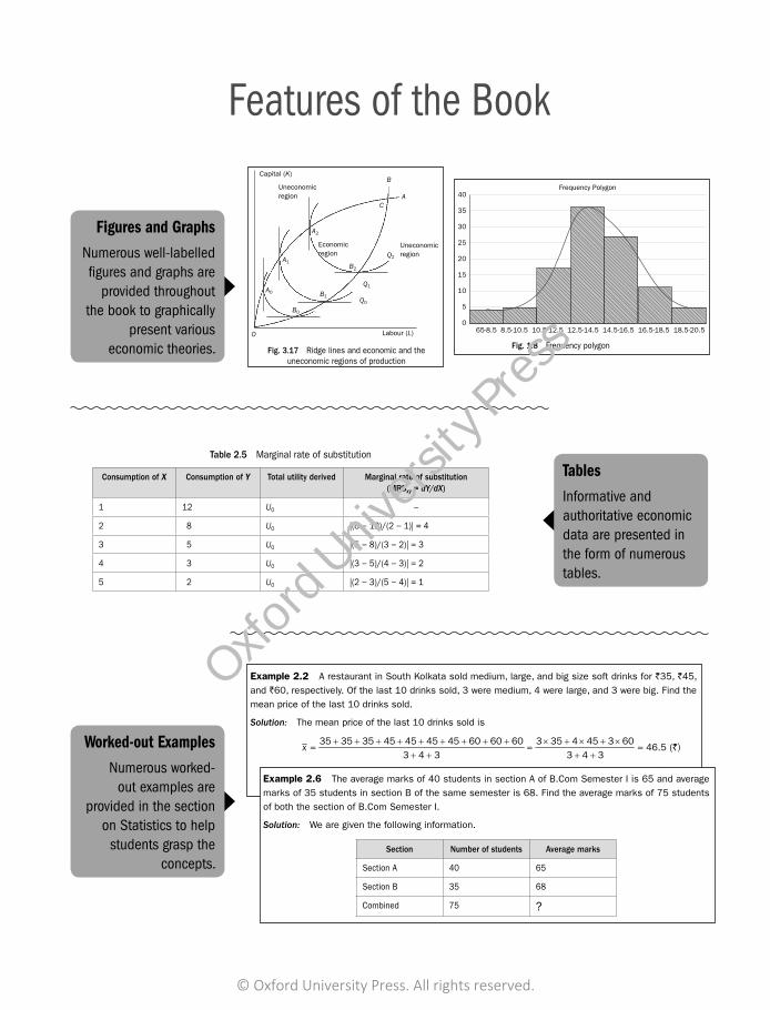
Figures and Graphs Numerous well-labelled figures and graphs are
provided throughout the book to graphically
present various economic theories.
Worked-out ExamplesNumerous worked-
out examples are provided in the section
on Statistics to help students grasp the
concepts.
TablesInformative and authoritative economic data are presented in the form of numerous tables.
Fundamentals 167
Example 1.16 Consider the data given in Table 1.19 and draw a frequency polygon of it.
Table 1.19
Class interval Frequency
6.5–8.5 4
8.5–10.5 5
10.5–12.5 17
12.5–14.5 36
14.5–16.5 27
16.5–18.5 11
18.5–20.5 5
Solution: First, we need the mid-point of the class interval. This is found as given in Table 1.20.
Table 1.20
Class interval Mid-point Frequency
6.5–8.5 7.5 4
8.5–10.5 9.5 5
10.5–12.5 11.5 17
12.5–14.5 13.5 36
14.5–16.5 15.5 27
16.5–18.5 17.5 11
18.5–20.5 19.5 5
The frequency polygon obtained is shown as the curve in Fig. 1.8.
065-8.5 8.5-10.5 10.5-12.5
Frequency Polygon
12.5-14.5 14.5-16.5 16.5-18.5 18.5-20.5
5
10
15
20
25
30
35
40
Fig. 1.8 Frequency polygon
Economics_Ch06.indd 167 13/06/17 2:55 PM
Theory of Production 73
capital, it will have to use more labour as well tokeep the total production constant. Consequently,beyond point A0, isoquant Q0 will be positivelysloped. The firm will obviously not produce in this range, since the marginal productivity of capitalis negative and it is not profitable for the firmto use capital anymore. Therefore, this range isthe uneconomic range of production. Similarly,at point B0, use of labour reaches the maximumlevel. In other words, at point B0, the marginalproductivity of labour is zero. Beyond point B0, the marginal productivity of labour becomesnegative and, therefore, if the firm wishes to usemore labour, it will have to use more capital also tokeep the total production constant. Consequently,beyond point B0, isoquant Q0 will be positivelysloped. The firm will obviously not produce in this
range, since marginal productivity of labour is negative and it is not profitable for the firmto use labour anymore. Therefore, this range is also the uneconomic range of production.Similarly, we get points such as A1 and B1 on isoquant Q1 and A2 and B2 on isoquant Q2, beyond which the isoquants become positively sloped. Locus of all points such as A0, A1, and A2, that is, OA, is called the upper ridge line where the marginal productivity of capitalbecomes zero. On the other hand, locus of all points such as B0, B1, and B2, that is, OB, iscalled the lower ridge line, where the marginal productivity of labour becomes zero. Ridgeline is, thus, the locus of all such factor combinations where marginal product of any one ofthe two factors becomes zero. To the left of the upper ridge line and to the right of lowerridge line, marginal productivity of one of the two factors becomes negative and, therefore,it is not profitable for the firm to produce in these regions. Hence, upper ridge line andlower ridge line are the boundary lines between the economic region and the uneconomicregions of production.
If the firm continues to move on higher isoquants, substitutability of two factors decreases gradually. As a result, the convex to the origin portion of the successively higher isoquants decreases. Therefore, the upper and lower ridge lines OA and OB approach one another and ultimately they intersect at point C. Point C is known as the Bliss Point, at which the firm reachesthe maximum possible level of output.
3.14 Isocost LineThe cost of production is extremely important in conducting production. Isocost line is the locusof all such factor input combinations for which the total cost of production remains constant. Inother words, an isocost line shows the different combinations of factors of production that can be employed with a given total cost. Let us take an example as shown in Table 3.4. Suppose that a producer has a total budget of `120, and for producing a certain level of output, he/she has
Fig. 3.17 Ridge lines and economic and the uneconomic regions of production
Labour (L)
Q0
B0
B1
B2
A2
A1
A0
Q1
Q2
A
B
C
Capital (K)
Uneconomic region
Economic region
Uneconomic region
O
Economics_Ch03.indd 73 6/5/2017 12:33:01 PM
Theory of Consumer Behaviour 39
away less and less units of Y so that the marginal rate of substitution falls from 4 to 1 in the fifth combination. The aforementioned five combinations of X and Y are actually the points A, B, C, D, and E on the indifference curve IC0 as shown in Fig. 2.9.
Therefore, it is proved that as the consumer proceeds from upward left to downward right along the same indifference curve, the marginal rate of substitution diminishes. The diminishingmarginal rate of substitution between two goods is the property of a convex to the origin curve. Therefore, the indifference curve is convex to the origin. In case of a negatively sloped straight line, the marginal rate of substitution is constant and in case of a concave to the origin curve, the marginal rate of substitution is increasing.
Two Indifference Curves Can Never Touch or Intersect Each Other
To prove this property, let us assume that two indifference curves can touch or intersect each other.In Fig. 2.10, two indifference curves IC0 and IC1 touch each other at point B. A and B are
two points on the indifference curve IC0 and B and C are two points on the indifference curve IC1. Therefore, consumer is indifferent between A and B and also between B and C. Accordingto the axiom of transitivity, the consumer should be indifferent between A and C. However, this is impossible, because point C has more of both the commodities X and Y than point A.
Table 2.5 Marginal rate of substitution
Consumption of X Consumption of Y Total utility derived Marginal rate of substitution (MRSxy = dY/dX)
1 12 U0 –
2 8 U0 |(8 − 12)/(2 − 1)| = 4
3 5 U0 |(5 − 8)/(3 − 2)| = 3
4 3 U0 |(3 − 5)/(4 − 3)| = 2
5 2 U0 |(2 − 3)/(5 − 4)| = 1
1 2 3 4 5
12
8
A
B
C
O
D
E
IC0
5
3
2
Commodity X
Commodity Y
Fig. 2.9 Convexity of indifference curve
Commodity X
Commodity Y
A
C
B
O
IC1
IC0
Fig. 2.10 Two indifference curves touching each other
Economics_Ch02.indd 39 6/5/2017 12:27:34 PM
2 Microeconomics 1 and Statistics
2.2.1 Arithmetic MeanThe arithmetic mean (AM), or mean, of a variable is the sum of all the values in the data set of the variable divided by the number of units of that variable in the data set. Arithmetic mean is of two types: unweighted or simple arithmetic mean and weighted arithmetic mean.
Unweighted Arithmetic Mean The unweighted arithmetic mean is the simple sum of the values of a set of observations of a variable divided by the number of observations. If we have n values of a variable x as x1, x2, ...,xn, the unweighted arithmetic mean or, simple mean, denoted by x, is:
=+ + + += =
∑1 2 3 1...
n
in i
xx x x x
xn n
(2.1)
Example 2.1 The daily wages (in ̀ ) of 10 workers in a factory are as follows: 240, 275, 265, 270, 400,480, 670, 850, 550, and 250. Calculate the mean wage of the workers.
Solution: Mean wage = `425[Note: unit of measurement (in this example `) should be given in the answer]
Weighted Arithmetic MeanThe weighted mean occurs when there are several observations of the same value. To explain weighted mean consider the following example:
Example 2.2 A restaurant in South Kolkata sold medium, large, and big size soft drinks for `35, `45, and `60, respectively. Of the last 10 drinks sold, 3 were medium, 4 were large, and 3 were big. Find the mean price of the last 10 drinks sold.
Solution: The mean price of the last 10 drinks sold is
+ + + + + + + + + × + × + ×= = =
+ + + +35 35 35 45 45 45 45 60 60 60 3 35 4 45 3 60
46.5 (3 4 3 3 4 3
x `)
In this example, the weights are frequency counts. Weighted arithmetic mean is related to a frequency distribution. If the ith observation of a variable x is xi and its frequency is fi, then weighted arithmetic mean is defined as
=+ + + += =
+ + + +
∑��
1 1 2 2 3 3 1
1 2 3
n
i in n i
n
f xf x f x f x f x
xf f f f N
(2.2)
All possible values of a variable form what is knownas population distribution and the mean of thisdistribution is the population mean. Population isa theoretical distribution and its mean is a parameterwhich is unknown and we need to estimate it witha sample drawn from this population. A sampleis a part of the population and its mean is the
sample mean which is called statistic. Populationrepresents the universal set, while the sample is aset drawn from this universal set. Any measurablecharacteristic of a population is called a parameter.The mean of a population is a parameter. The meanof a sample, or any other measure based on sampledata, is called a statistic.
Economics_Ch02.indd 2 09-06-2017 16:23:10
Measures of Central Tendency 5
Proof: Let the variable x has n1 + n2 observations xi, i = 1, 2, …, n1 + n2, which is decomposed into 2 sets xj, j = 1, 2, … n1, and xk, k = 1, 2, …, n2. Therefore, we can write
1 2 1 2
1 1 1
n n n n
i j ki j k
x x x+
= = == +∑ ∑ ∑
Or, ( ) ( )1 2 1 2
1 2 1 2 1 1 2 21 1 1
/ / /n n n n
i j ki j k
n n x n n n x n n x n+
= = =+ + = +∑ ∑ ∑
Or, ( )1 2 1 1 2 2n n x n x n x+ = +
Or, 1 1 2 2
1 2
n x n xxn n+
=+
The composite mean lies between the group means, that is, ≤ ≤1 2x x x .
Example 2.6 The average marks of 40 students in section A of B.Com Semester I is 65 and average marks of 35 students in section B of the same semester is 68. Find the average marks of 75 students of both the section of B.Com Semester I.
Solution: We are given the following information.
Section Number of students Average marks
Section A 40 65
Section B 35 68
Combined 75 ?
Here, n1 = 40, n2 = 35, n1 + n2 = 75, 1x = 65, and 2x = 68
Now, + × + ×= = =
+1 1 2 2
1 2
40 65 35 6866.4
75n x n x
xn n
Calculation of AM for Frequency DistributionDiscrete series Let us consider the following frequency distribution of a variable x. Here, xi
and fi denote the value of the variable and the corresponding frequency for observation unit i.
xi fi fi xi
x1 f1 f1x1
x2 f2 f2x2
x3 f3 f3x3
. . .
. . .
. . .
xn fn fnxn
Total1
n
ii
f=∑
1
n
i ii
f x=∑
Economics_Ch02.indd 5 09-06-2017 16:23:18
Microeconomics.indb 12 6/21/2017 6:43:21 PM
© Oxford University Press. All rights reserved.
Oxford
Universi
ty Pre
ss

Question BankNumerous additional
solved questions with answers are
provided in a question bank for students to
prepare themselves for examinations.
ExercisesExhaustive chapter-end exercises are provided for the students to practice the concepts.
Solved CU Question Papers/Model Question PapersStudents can learn from solved previous years’ University question papers and attempt the model question papers for themselves.
Theory of Consumer Behaviour 53
[According to CU syllabus of Economic-I paper for B Com Honours and General, third unit requires 10 lectures and 12 marks. Therefore, we have incorporated the short-answer type questions carrying two marks, medium-answer type questions carrying four
marks, and broad-answer type questions carrying eight marks in the exercise.]
SHORT-ANSWER TYPE QUESTIONS (2 MARKS)
1. What do you mean by marginal utility? 2. What would be the value of marginal utility when total
utility is maximum? [CU B Com (G), 2008] 3. What are the consumer’s equilibrium conditions in
Marshallian theory?4. What is net utility?5. What do you mean by the law of diminishing marginal
utility?6. If marginal utility is higher than the price of the
commodity, what will the consumer do?7. If marginal utility is less than the price of the
commodity, what will the consumer do?8. What is the cardinal measurement of utility?9. What is consumer’s surplus? [CU B Com (G), 2009]
10. State two limitations of cardinal utility theory.11. Distinguish between cardinal utility and ordinal utility.
[CU B Com (G), 2013]12. What are the basic axioms of choice?13. What do you mean by an indifference curve?14. What are the characteristics of an indifference curve?
[CU B Com (G), 2007]15. What do you mean by marginal rate of substitution?
[CU B Com (G), 2007] 16. State the law of diminishing marginal rate of substitution.
17. What is an indifference map? 18. What do you mean by a budget line? 19. What are the conditions required to achieve consumer’s
equilibrium in indifference curve theory? [CU B Com (G), 2013]
20. What is a price–consumption curve? [CU. B Com (G), 2010]
21. What is an income–consumption curve?22. What do you mean by price effect?23. What do you mean by substitution effect?24. What do you mean by income effect?25. What is the relationship between price effect,
substitution effect, and income effect?26. Are all inferior goods called Giffen goods?
[CU B Com (G), 2006]27. What is the difference between ‘Giffen good’ and
‘inferior good’? [CU B Com (G), 2008]28. What does the demand curve for a normal good look
like?29. What is the shape of the demand curve for an inferior
good?30. What is the shape of the demand curve for a Giffen
good?
MEDIUM-ANSWER TYPE QUESTIONS (4 MARKS)
1. What are the basic assumptions of cardinal utility theory?
2. Explain the law of diminishing marginal utility.
3. What is the relation between the marginal utility curve and demand curve in Marshallian theory?
as a result of income effect. However, unlike the caseof inferior goods, income effect of a Giffen good is stronger than the substitution effect; therefore, the resultant effect goes against the direction of the substitution effect. In other words, as price falls,demand for Giffen good decreases and vice versa.
• While the demand curve for a normal good is negativelysloped, the demand curve for an inferior good is also
negatively sloped but steeper than that of a normal good. On the contrary, the demand curve for a Giffen good is positively sloped.
• Indifference curve theory is better than Marshallian theory in the sense that the former can explain the exceptions to the law of demand, that is, the cases ofinferior and Giffen goods, whereas the latter cannot do that.
E X E R C I S E S
Economics_Ch02.indd 53 6/5/2017 12:27:56 PM
Theory of Consumer Behaviour 53
[According to CU syllabus of Economic-I paper for B Com Honours and General, third unit requires 10 lectures and 12 marks. Therefore, we have incorporated the short-answer type questions carrying two marks, medium-answer type questions carrying four
marks, and broad-answer type questions carrying eight marks in the exercise.]
SHORT-ANSWER TYPE QUESTIONS (2 MARKS)
1. What do you mean by marginal utility?2. What would be the value of marginal utility when total
utility is maximum? [CU B Com (G), 2008]3. What are the consumer’s equilibrium conditions in
Marshallian theory?4. What is net utility?5. What do you mean by the law of diminishing marginal
utility?6. If marginal utility is higher than the price of the
commodity, what will the consumer do?7. If marginal utility is less than the price of the
commodity, what will the consumer do?8. What is the cardinal measurement of utility?9. What is consumer’s surplus? [CU B Com (G), 2009]
10. State two limitations of cardinal utility theory.11. Distinguish between cardinal utility and ordinal utility.
[CU B Com (G), 2013]12. What are the basic axioms of choice?13. What do you mean by an indifference curve?14. What are the characteristics of an indifference curve?
[CU B Com (G), 2007]15. What do you mean by marginal rate of substitution?
[CU B Com (G), 2007] 16. State the law of diminishing marginal rate of substitution.
17. What is an indifference map?18. What do you mean by a budget line?19. What are the conditions required to achieve consumer’s
equilibrium in indifference curve theory? [CU B Com (G), 2013]
20. What is a price–consumption curve? [CU. B Com (G), 2010]
21. What is an income–consumption curve?22. What do you mean by price effect?23. What do you mean by substitution effect?24. What do you mean by income effect?25. What is the relationship between price effect,
substitution effect, and income effect?26. Are all inferior goods called Giffen goods?
[CU B Com (G), 2006]27. What is the difference between ‘Giffen good’ and
‘inferior good’? [CU B Com (G), 2008]28. What does the demand curve for a normal good look
like?29. What is the shape of the demand curve for an inferior
good?30. What is the shape of the demand curve for a Giffen
good?
MEDIUM-ANSWER TYPE QUESTIONS (4 MARKS)
1. What are the basic assumptions of cardinal utility theory?
2. Explain the law of diminishing marginal utility.
3. What is the relation between the marginal utility curve and demand curve in Marshallian theory?
as a result of income effect. However, unlike the caseof inferior goods, income effect of a Giffen good is stronger than the substitution effect; therefore, the resultant effect goes against the direction of the substitution effect. In other words, as price falls,demand for Giffen good decreases and vice versa.
• While the demand curve for a normal good is negativelysloped, the demand curve for an inferior good is also
negatively sloped but steeper than that of a normal good. On the contrary, the demand curve for a Giffen good is positively sloped.
• Indifference curve theory is better than Marshallian theory in the sense that the former can explain the exceptions to the law of demand, that is, the cases ofinferior and Giffen goods, whereas the latter cannot do that.
E X E R C I S E S
Economics_Ch02.indd 53 6/5/2017 12:27:56 PM
54 Microeconomics 1 and Statistics
4. What are the two basic conditions required for equilibrium of the consumer in cardinal utility theory?
5. What are the basic limitations of Marshallian cardinal utility theory?
6. Explain the axioms of choice in ordinal utility theory.7. What do you mean by an indifference curve? What are
the properties of an indifference curve?8. What is an indifference curve? State two of its properties.
[CU B Com (G), 2011]9. Prove that an indifference curve is always negatively sloped.
10. Prove the law of diminishing marginal rate of substitution.
11. Prove that the two indifference curves can never touch or intersect each other.
12. What is an indifference map? Explain two properties of an indifference curve.
13. What is a budget line? Explain the shifts of a budget line.14. What is income–consumption curve? What would be
the shape of an income–consumption curve if one of the two goods is inferior?
15. What is price–consumption curve? How can you draw a price–consumption curve?
16. Define ‘price effect’. Distinguish between ‘price effect’ and ‘substitution effect’. [CU B Com (G), 2012]
17. Prove that all Giffen goods are inferior goods but all inferior goods are not Giffen goods.
18. Explain the differences between the demand curve for a normal good, demand curve for an inferior good, and demand curve for a Giffen good.
19. Why indifference curve theory is better than Marshallian cardinal utility theory?
LONG-ANSWER TYPE QUESTIONS (8 MARKS)
1. Explain the law of diminishing marginal utility. 2. Distinguish between total utility and marginal utility
with the help of a suitable diagram.3. How the demand curve can be derived with the help of
Marshallian marginal utility curve?4. What is consumer’s surplus? Explain how can you
measure Marshallian consumer’s surplus?5. What are the limitations of Marshallian cardinal utility
theory?6. Table 2.8 portrays Puja’s total utility from consumption
of chocolates. The column for marginal utility has been left blank. Calculate the values for marginal utility and fill in the blanks in the marginal utility column.
Table 2.8 Total utility from consumption of chocolates
No. of chocolates Total utility Marginal utility
0 0 –
1 50 –
2 100 –
3 140 –
4 170 –
5 190 –
Does Puja experience the law of diminishing marginal utility from consuming chocolates?How do you know?
7. What are the axioms of choice in the ordinal utility theory?
8. What is an indifference curve? Derive indifference curve with the help of a suitable diagram.
9. What is an indifference map? Explain the properties of an indifference curve. [CU B Com (G), 2005]
10. What is a budget line? Explain the shifts of a budget line.11. Discuss the characteristics of an indifference curve. How
would you explain the consumer’s equilibrium under indifference curve analysis? [CU B Com (G), 2008]
12. Table 2.9 portrays Puja’s consumption of different combinations of two commodities—chocolates and sweets—where total utility remains constant. Calculate the marginal rate of substitution of sweets for chocolates and fill in the blanks in the marginal rate of substitution column.
Table 2.9 Different consumption combinations of chocolates and sweets
Commodity bundle
Consumption of chocolates
Consumptionof sweets
Total utility
derived
Marginal rate of
substitution
A 15 1 U0 –
B 10 2 U0 –
C 6 3 U0 –
D 3 4 U0 –
E 1 5 U0 –
Economics_Ch02.indd 54 6/5/2017 12:27:56 PM
Question Bank – Microeconomics IMULTIPLE-CHOICE TYPE QUESTIONS
1. If the demand for a good is inelastic, an increase in its price will cause the total expenditure of the consumers of the good to
(a) increase(b) decrease(c) remain the same(d) become zero
2. The horizontal demand curve implies that the elasticity of demand is
(a) zero(b) infinite(c) equal to one(d) greater than zero but less than infinity
3. Each point on the demand curve reflects(a) the highest price consumers are willing and able
to pay for that particular unit of a good. (b) the highest price sellers will accept for all units
they are producing. (c) the lowest-cost technology available to produce a
good.(d) all the wants of a given household.
4. A substitute is a good(a) of higher quality than another good.(b) that can be used in place of another good. (c) that is not used in place of another good. (d) of lower quality than another good.
5. A complement is a good(a) used in conjunction with another good. (b) of lower quality than another good. (c) used instead of another good.(d) of higher quality than another good.
6. A normal good is a good for which (a) there are very few complements. (b) demand decreases when income increases. (c) demand increases when income increases. (d) there are few substitutes.
7. An increase in demand combined with no change in supply causes
(a) a decrease in demand because the supply curve does not shift.
(b) the equilibrium price to fall.
(c) a movement rightward along the demand curve.
(d) the equilibrium price to rise. 8. Which of the following will always raise the equilibrium
price? (a) an increase in demand combined with a decrease
in supply (b) a decrease in both demand and supply(c) an increase in both demand and supply(d) a decrease in demand combined with an increase
in supply 9. If a decrease in the price of gasoline increases the
demand for large cars, then (a) gasoline and large cars are complements in
consumption. (b) large cars are an inferior good.(c) gasoline is an inferior good.(d) gasoline and large cars are substitutes in
consumption. 10. A utility function that describes how much of a basket
of goods is preferred to another is called (a) an ordinal utility function.(b) a cardinal utility function.(c) a utility-maximizing function. (d) a definitive utility function.
11. Indifference curves cannot intersect because of the assumption that
(a) marginal utility diminishes as more of that good is consumed.
(b) indifference curves are negatively sloped.(c) preferences are transitive. (d) preferences are complete.
12. Indifference curves cannot slope upward because of the assumption that
(a) MRS is in absolute value.(b) more is preferred to less(c) preferences are transitive. (d) preferences are complete.
13. Marginal utility refers to(a) the additional product produced as the firm adds
one additional unit of an input.
Economics_Question_Bank_Part1.indd 135 6/21/2017 6:38:50 PM
B.Com Examination 2014
(New Syllabus)
Economics-I Solved Relevant Question Paper
Fourth Paper [C-14G] Full Marks-100
Module-I
Group-A
1. Answer the following questions: 2 × 5
(a) State any two characteristics of business economics.Ans. Two important characteristics of business economics are:
(i) Microeconomics: Business economics is micro economic in character. This is so because it studies the problems of an individual business unit. It does not study the problems of the entire economy.
(ii) Also uses macroeconomics: Although business economics is micro economic in nature, marco economics is also useful to business economics. Macroeconomics provides an intelligent understanding of the environment in which the business operates. Business economics takes the help of macro-economics to understand the external conditions such as business cycle, national income, economic policies of Government etc.
(b) How do you measure slope of a curve at a point?
Or
What is meant by a budget line?Ans. The slope of a curve is defined as the change in the value of the variable on the y-axis divided by the
change in the value of the variable on the x-axis. The formula for slope is ∅∅
yx
, where D means ‘change
in’. A curve has a varying slope, which can be calculated by drawing a straight line tangent to the curve at that point and then calculating the slope of the line. To calculate the slope of the curve at any point, we draw a straight line tangent to the curve at that point and then calculate the slope of the line. We can take example of total cost curve, which is first inverted U-shaped and then U-shaped. We calculate the slope of the curve at two different points in Figure 1.
AF E
C
D
B
H G Total output
Total cost
Figure 1 Slope of the total cost curve
Economics_Part I_Solved_Model_Questions_2014.indd 1 6/14/2017 11:03:37 AM
Model Question Paper-1Statistics
Full Marks-50
Group A1. Answer the following questions: 5 × 2 = 10
(a) Type of cumulative frequency distribution in which class intervals are added in top to bottom order is classified as(i) variation distribution(ii) less than type distribution(iii) more than type distribution(iv) marginal distribution
(b) What are the differences between an attribute and a variable?OrWhat is the most appropriate measure of central tendency when the data has outliers?
(c) The mean of 100 observations is 50 and their standard deviation is 5. The sum of all squares of all the observations is(i) 50000(ii) 250000
(iii) 252500(iv) 255000
(d) Moment about mean which is indication whether distribution is symmetrical or asymmetrical is considered as(i) first moment(ii) third moment(iii) second moment(iv) fourth momentOr,If y is a polynomial of nth degree and the nth differences are constant, what will be the value of differences of higher order?
(e) State Lagrange’s interpolation formula.
Group B2. Answer the following questions. 5 × 4 = 20
(a) What are the main sources of secondary data?
(b) Draw a line graph from the following data:
Year 1924 1925 1926 1927 1928 1929 1930
Monthly 609 522 205 608 551 632 516
Average
Production
Or, The mean age of a group of people is 30 years. If the mean age of men is 32 and that of women is 27 in the group, find out the percentage of men and women in the group.
(c) While calculating the mean and variance of 10 readings, a student wrongly used the reading 52 for the correct reading 25. He obtained the mean and variance as 45 and 16 respectively. Find the correct mean and the varianceOrThere were five customer service representatives on duty at the Electronic Super Store during last weekend’s sale. The numbers of HDTVs these representatives sold are: 5, 8, 4, 10, and 3. Calculate mean deviation.
(d) Prove that the coefficient of skewness is the 3rd order standardized raw moment.Or Explain D5y0 in terms of y0, y1, y2, …Or, Form a simple frequency distribution with the following:7,4,3,5,6,3,3,2,4,3,4,3,3,4,4,3,2,2,4,3,5,4,3,4,3,4,3,1,2,3.
Economics_Part II_Model_Questions_1.indd 1 6/14/2017 7:23:49 PM
Microeconomics.indb 13 6/21/2017 6:43:22 PM
© Oxford University Press. All rights reserved.
Oxford
Universi
ty Pre
ss

Road Map—University of Calcutta SyllabusModule I: Microeconomics I
UNIT TOPIC DETAILS CHAPTER
Unit I Demand and consumer behaviour
Concept of demand, demand function, law of demand, derivation of individual and market demand curves, shifting of the demand curve; elasticity of demand.
Consumer behaviour: Marshallian utility approach and indifference curve approach; utility maximization conditions; income–consumption curve (ICC) and price–consumption curve (PCC), derivation of demand curve from PCC.
1
2
Unit II Production and cost
Production function: Short-run and long-run; relation among total product, average product and marginal product, law of returns to a variable factor, law of returns to scale; concepts of isoquant and isocost line; conditions for optimization (graphical approach).
Cost: Accounting and economic costs; social and private costs; short-run and long-run costs; relation between average and marginal costs; determination of LAC curve from SAC curves, LMC.
3
4
Unit III Perfect competition
Concept of perfectly competitive market: Assumptions, profit maximization conditions; related concepts of total revenue, average revenue and marginal revenue, short-run and long run equilibrium of a firm; determination of short-run supply curve of a firm, measuring producer surplus under perfect competition, Stability analysis—Walrasian and Marshallian, demand supply analysis including impact of taxes and subsidy.
5
Module II: StatisticsUNIT TOPIC DETAILS CHAPTER
Unit I Fundamentals Definition of statistics, scope and limitation of statistics, attribute and variable, primary and secondary data, method of data collection, tabulation of data, graphs and charts, frequency distribution, diagrammatic presentation of frequency distribution
1
Unit II Measures of central tendency
Meaning of central tendency, common measures – mean (AM, GM, HM), median, and mode, Partition values—quartiles, deciles, and percentiles, applications of different measures.
2
Unit III Measures of dispersion
Meaning of dispersion, common measures—range, quartile deviation, mean deviation, and standard deviation; relative measures of dispersion, combined standard deviation, applications of different measures.
3
Unit IV Moments, skewness, and kurtosis
Different types of moments and their relationships, meaning of skewness and kurtosis, different measures of skewness, measure of kurtosis, applications of different measures.
4
Unit V Interpolation Finite differences, polynomial function, Newton’s forward and backward interpolation formula, Lagrange’s interpolation formula.
5
Microeconomics.indb 14 6/21/2017 6:43:23 PM
© Oxford University Press. All rights reserved.
Oxford
Universi
ty Pre
ss

CHAPTER
1Basics of Demand
This chapter provides the ideas about the concept of demand, law of demand, factors determining demand and demand function. It discusses construction of demand schedule and derivation of individual and market demand curve. The chapter elaborates the difference between movements along the demand curve and shifting of demand curve. It states the situations of exceptions to the law of demand.
1.1 IntroductionOne of the best ways to start discussing about the fundamentals of economics is to begin with the basics of demand and supply. Supply–Demand analysis is a fundamental and powerful tool that can be applied to a wide variety of important problems of economics. We try to ascertain how demand and supply curves are used to describe the market mechanism. Supply and demand come into equilibrium to determine both market price of a good and the total quantity produced. What the market price and quantity will be depends on the particular characteristics of supply and demand. We will therefore discuss the basic concepts and characteristics of supply and demand in this chapter.
1.2 Demand FunctionDemand is the consumer’s willingness to get goods or service in exchange for a price. In other words, demand is a quantity of a commodity the consumer wants to purchase at a given price income situation. Demand depends on many factors. The functional relationship between the quantity demanded for a commodity and its determining factors is known as the demand function.
Demand function is the behavioural relationship between quantity demanded for a good or service and all the factors that influence the demand for that good or service. The major factors affecting the demand for a certain good or service are own price of the good or service, price of a substitute or complement of the good or service, personal disposable income, tastes and preferences, and consumer’s expectations about future prices and future income. The functional relationship between quantity demanded and its determinants is called the demand function.
Microeconomics.indb 3 6/21/2017 6:43:25 PM
© Oxford University Press. All rights reserved.
Oxford
Universi
ty Pre
ss

4 Microeconomics 1 and Statistics
Demand function can be written as follows:
QD = f (P, P/, YD, T, EP, Ey) (1.1)
where P = own price of the good or service, P/ = price of a substitute or complement of the good or service YD = personal disposable income, T = tastes and preferences, EP = expectations about future prices, and Ey = expectations about future income. The factors affecting demand are as follows.
Own price of the good or service The basic demand relationship is between different prices of a good or service and the quantities that would be purchased at those prices. Generally, such a relationship is negative, that is, an increase in price will induce a decrease in the quantity demanded.
Price of related goods or services Related goods of the primary good are of two types, that is, complements and substitutes. Complements are goods that are used with the primary good. For example, tea and sugar are complementary goods. To consume tea, one must also consume sugar. If the price of sugar goes up, the quantity demanded for tea goes down automatically. The mathematical relationship between the price of the complement and the demand for the good in question, is negative. The other main category of related goods is substitute. Substitutes are goods that can be used in place of the primary good. For example, tea and coffee. Coffee can be consumed in place of tea. Therefore, if the price of coffee goes down, people will start consuming more coffee and automatically demand for tea will go down. The mathematical relationship between the price of the substitute and the demand for the good in question, is positive.
Consumers’ income In general, the more income (income after tax) a person has, the more likely that person is willing to buy the particular good or service. Therefore, the mathematical relationship between income and the demand for the good or service in question, is positive.
Tastes and preferences How much of a particular good or service is demanded also depends on an individual’s taste and preference for the item. In general, economists use the term ‘tastes and preferences’ as a comprehensive category for a consumer’s attitude towards a product. In this sense, if due to a change in fashion, habit etc., a consumer’s taste and preference for a particular good or service increases, the quantity demanded increases, and vice versa. Therefore, the mathematical relationship between tastes and preferences for a good or service and the demand for the good or service in question is positive.
Consumer’s expectations about future prices and income If a consumer believes that the price of the good or service will be higher in the future, he/she is more likely to purchase the good or service now. Therefore, the mathematical relationship between the consumer’s expectations about future prices of the good or service and the demand for the good or service is positive. If the consumer expects that his/her income will be higher in the future, the consumer is less likely to buy the good or service now.
In Eq. (1.1), dQD/dP < 0 (since, mathematical relationship between the price of the good and the demand for it, is negative), dQD/dP/ > 0 for substitute (since, mathematical relationship
Microeconomics.indb 4 6/21/2017 6:43:25 PM
© Oxford University Press. All rights reserved.
Oxford
Universi
ty Pre
ss

Basics of Demand 5
between the price of the substitute and the demand for the good in question, is positive), dQD/dP/ < 0 for complement (since, mathematical relationship between the price of the complement and the demand for the good in question is, negative), dQD/dYD > 0 (since, mathematical relationship between the income of the consumer and the demand for the good, is positive), dQD/dT > 0 (since, mathematical relationship between the tastes and preferences for the good and the demand for the good, is positive), dQD/dEP > 0 (since, mathematical relationship between expectations about future prices and the demand for the good, is positive), and dQD/dEY < 0 (since, mathematical relationship between expectations about future income and the demand for the good, is negative).1
1.3 The Law of DemandDemand for a commodity depends on so many factors such as its own price, price of other commodities, and so on. The law of demand states that the quantity demanded for a commodity increases when its price falls and vice versa, if all other factors remain the same. The inverse relation between quantity demanded for a commodity and its own price under ceteris paribus assumption is known as the law of demand.
In other words, the law of demand states that the quantity demanded and the price of a commodity are inversely related, other things remaining constant. All the goods, for which law of demand is applicable, are called normal goods. The reason behind the inverse relationship between quantity demanded and price for a normal good is quite simple. People have limited incomes. Suppose, a consumer purchases 1 kg of apple for consumption of his/her family for 1 week. If the price of apple goes up, the weekly expenditure of the consumer for apple will also go up if he/she continues to purchase the same quantity after the rise in price. In order to maintain the weekly budget, the consumer will reduce his/her consumption for apple. The opposite thing will happen if the price of apple goes down. Therefore, it is clear, for normal goods, if price goes up, quantity demanded will go down and vice versa. The geometric representation of price quantity relationship is known as the demand curve. The law of demand suggests that the demand curve for a commodity should be negatively sloped.
However, law of demand implies that changing price would move quantity demanded up or down, but this would not change the demand itself. Change in quantity demanded and change in demand are not the same concept. Change in quantity demanded refers to the change in the amount of a commodity as a result of change in the price of it. Amount demanded rises or falls according to the fall or rise in price. In such a case, other factors influencing demand are held constant. The change takes place in the same demand curve. On the other hand, ‘change in demand’ means changes in demand due to the changes in the factors other than price, for example, income, taste and preference, prices of other related
1dQD/dP = Change in quantity demanded due to change in own price dQD/dP/ = Change in quantity demanded due to change in price of substitute or complement dQD/dYD = Change in quantity demanded due to change in disposable income dQD/dT = Change in quantity demanded due to change in tastes and preferences dQD/dEP = Change in quantity demanded due to change in expectation about future price dQD/dEY = Change in quantity demanded due to change in expectation about future income
Microeconomics.indb 5 6/21/2017 6:43:25 PM
© Oxford University Press. All rights reserved.
Oxford
Universi
ty Pre
ss

6 Microeconomics 1 and Statistics
commodities, etc. The change in demand involves ‘increase’ and ‘decrease’ of the demand for a commodity. In case of change in demand the entire demand schedule and demand curve change. With an increase in demand, the curve shifts upwards and with a decrease in demand, the curve shifts downwards.
1.3.1 Demand ScheduleA demand schedule is crucial for constructing a demand curve. A demand schedule lists prices and corresponding quantities based on the law of demand. To understand the concept of demand schedule better, let us look at the demand schedule of a popular luxury soap in Table 1.1.
It exhibits hypothetical demand schedule of an individual for a popular luxury soap. We find that there is an inverse relationship between price and quantity demanded because a demand schedule follows the law of demand.
1.3.2 Derivation of Individual Demand CurveWe can construct the demand curve of an individual for a luxury soap based on the demand schedule, as shown in Fig. 1.1. While deriving the demand curve, we would always measure quantity along the horizontal axis and price along the vertical axis. Demand curve is the locus of all the points showing demand for a good or service at various prices of that good or service. Table 1.1 shows that when the price is `50, the quantity demanded is 1 unit. Similarly, when the price is `40, the quantity demanded is 2 units, and so on. As we can see, there is a corresponding quantity for each price. By joining all the points established by plotting all prices and their corresponding quantities on a graph, we can obtain a demand curve. Hence, the demand curve for a normal good exhibits the law of demand, that is, the relationship between two variables, namely price and quantity demanded. Since the demand curve follows the law of demand, it is negatively sloped.
1.3.3 Derivation of Market Demand CurveThe previously discussed demand schedule and demand curve are the case of an individual. The analysis can be extended to a market in the same manner. A market typically consists of many customers and different customers possess different tastes and preferences, different incomes, different expectations about future prices and future incomes. Hence, individual demand curves differ from person to person in their slopes and shapes. However, we are able to sum up all individual demand curves and derive a market demand curve. In other words, the market demand curve is the sum of all individual demand curves.
For simplicity, let us assume that the market consists of only two customers. Table 1.2 depicts the individual demand schedules of a popular luxury soap for consumer 1 and consumer
Table 1.1 Demand schedule of luxury soap
Price (`) Quantity demanded
50 1
40 2
30 3
20 4
10 5
50
40
30
20
10
Price
Quantity0 1 2 3 4 5
D
D
Figure 1.1 Individual demand curve
Microeconomics.indb 6 6/21/2017 6:43:25 PM
© Oxford University Press. All rights reserved.
Oxford
Universi
ty Pre
ss

Basics of Demand 7
2 and also the combined demand schedule of the luxury soap for the market. From Table 1.2, we understand that the market demand is obtained by summing up individual demands. The table shows that at price `50, the market demand is 1 unit; at price ̀ 40, the market demand is 3 units; at price ̀ 30, the market demand is 5 units; and so on. Since there is an inverse relationship between price and quantity demanded, it is obvious that the market demand schedule also follows the law of demand.
Similarly, we can derive the market demand curve (D) by the horizontal summation of individual demand curves (D1 + D2), as illustrated in Fig. 1.2.
Table 1.2 Individual demand schedules of luxury soap
Price (`) Quantity demanded by Market demand of luxury soapConsumer 1 Consumer 2
50 1 0 1
40 2 1 3
30 3 2 5
20 4 3 7
10 5 4 9
50
40
30
20
10
0
Price
Quantity1 3 5 7 9
D
(c)
40
30
20
10
0
Price
Quantity1 2 3 4
D2
(b)
50
40
30
20
10
0
Price
Quantity1 2 3 4 5
D1
(a)
Figure 1.2 Demand curve (a) Demand curve for consumer 1 (D1) (b) Demand curve for consumer 2 (D2) and (c) Market demand curve (D1 + D2 = D)
P1
P2
P3
Price
QuantityO Q1 Q2 Q3
D
B
A
CD
Figure 1.3 Movements along the demand curve
1.3.4 Movement along the Demand CurveMovement along the demand curve occurs when there is a change in the own price. As we know, there is an inverse relationship between price and quantity demanded. Hence, reduction in the price causes a downward movement. This means that there is an increasing demand. Further, rise in the price causes an upward movement. This means that there is a decreasing demand. Movements along the demand curve are shown in Fig. 1.3.
In Fig. 1.3, the movement from A to C represents movement along the demand curve. At point A, the price is OP2 and the quantity demanded is OQ2. When there is a movement from point A to point C, price falls to OP3 and quantity demanded increases to OQ3. Further,
when there is a movement from point A to point B, price rises to OP1 and quantity demanded decreases to OQ1. Here, we can notice that the movement along the demand curve occurs because of a rise or a fall in the price level.
Microeconomics.indb 7 6/21/2017 6:43:25 PM
© Oxford University Press. All rights reserved.
Oxford
Universi
ty Pre
ss
8 Microeconomics 1 and Statistics
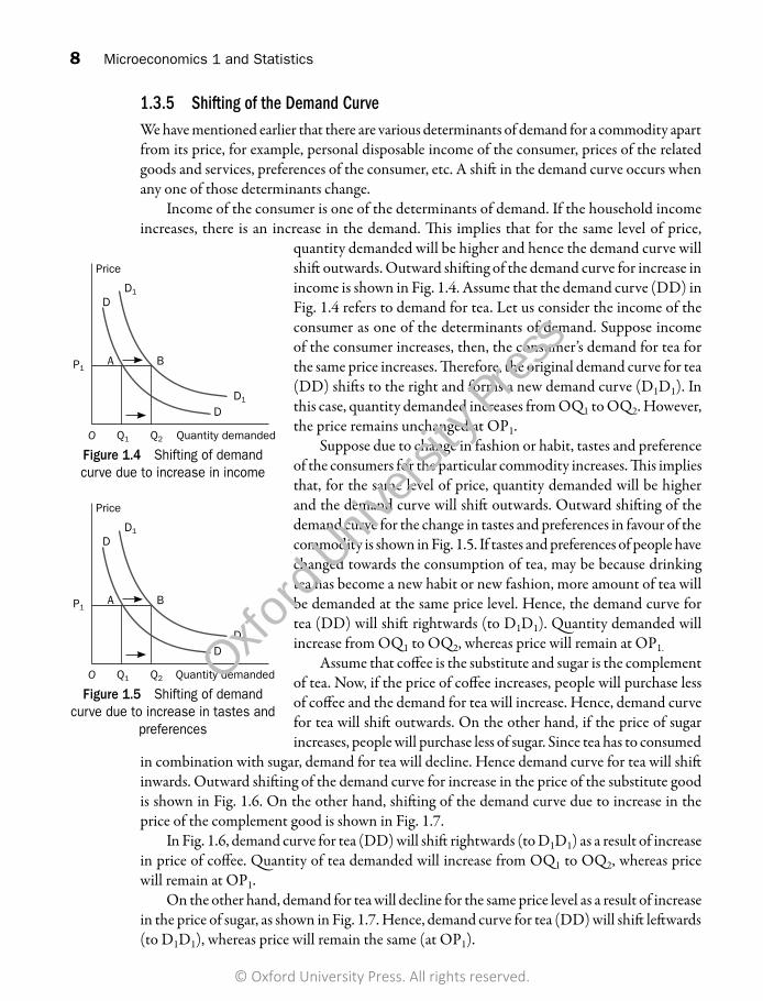
1.3.5 Shifting of the Demand CurveWe have mentioned earlier that there are various determinants of demand for a commodity apart from its price, for example, personal disposable income of the consumer, prices of the related goods and services, preferences of the consumer, etc. A shift in the demand curve occurs when any one of those determinants change.
Income of the consumer is one of the determinants of demand. If the household income increases, there is an increase in the demand. This implies that for the same level of price,
quantity demanded will be higher and hence the demand curve will shift outwards. Outward shifting of the demand curve for increase in income is shown in Fig. 1.4. Assume that the demand curve (DD) in Fig. 1.4 refers to demand for tea. Let us consider the income of the consumer as one of the determinants of demand. Suppose income of the consumer increases, then, the consumer’s demand for tea for the same price increases. Therefore, the original demand curve for tea (DD) shifts to the right and forms a new demand curve (D1D1). In this case, quantity demanded increases from OQ1 to OQ2. However, the price remains unchanged at OP1.
Suppose due to change in fashion or habit, tastes and preference of the consumers for the particular commodity increases. This implies that, for the same level of price, quantity demanded will be higher and the demand curve will shift outwards. Outward shifting of the demand curve for the change in tastes and preferences in favour of the commodity is shown in Fig. 1.5. If tastes and preferences of people have changed towards the consumption of tea, may be because drinking tea has become a new habit or new fashion, more amount of tea will be demanded at the same price level. Hence, the demand curve for tea (DD) will shift rightwards (to D1D1). Quantity demanded will increase from OQ1 to OQ2, whereas price will remain at OP1.
Assume that coffee is the substitute and sugar is the complement of tea. Now, if the price of coffee increases, people will purchase less of coffee and the demand for tea will increase. Hence, demand curve for tea will shift outwards. On the other hand, if the price of sugar increases, people will purchase less of sugar. Since tea has to consumed
in combination with sugar, demand for tea will decline. Hence demand curve for tea will shift inwards. Outward shifting of the demand curve for increase in the price of the substitute good is shown in Fig. 1.6. On the other hand, shifting of the demand curve due to increase in the price of the complement good is shown in Fig. 1.7.
In Fig. 1.6, demand curve for tea (DD) will shift rightwards (to D1D1) as a result of increase in price of coffee. Quantity of tea demanded will increase from OQ1 to OQ2, whereas price will remain at OP1.
On the other hand, demand for tea will decline for the same price level as a result of increase in the price of sugar, as shown in Fig. 1.7. Hence, demand curve for tea (DD) will shift leftwards (to D1D1), whereas price will remain the same (at OP1).
P1
Price
Quantity demandedO Q1 Q2
DD1
BA
DD1
Figure 1.4 Shifting of demand curve due to increase in income
P1
Price
Quantity demandedO Q1 Q2
DD1
BA
DD1
Figure 1.5 Shifting of demand curve due to increase in tastes and
preferences
Microeconomics.indb 8 6/21/2017 6:43:26 PM
© Oxford University Press. All rights reserved.
Oxford
Universi
ty Pre
ss

Basics of Demand 9
1.4 Exceptions to the Law of DemandFor most of the goods and services, according to the law of demand, the quantity demanded for a good increases with a decrease in price of the good and vice versa. Such goods and services are called normal goods and services. Demand curve for a normal good or service follows the law of demand and therefore it is downward sloping. In some cases, however, this may not be true. The circumstances when the law of demand becomes ineffective are known as exceptions of the law of demand. In those cases, the demand curve does not follow the law of demand and therefore it is not downward sloping. Such situations are explained in the following subsections.
1.4.1 Giffen GoodsSome special varieties of inferior goods are termed as Giffen goods. Cheaper varieties of this category like bajra, cheaper vegetable like potato come under this category. Sir Robert Giffen from Ireland first observed that people used to spend more of their income on inferior goods like potato and less of their income on meat. However, potatoes constituted their staple food. When the price of potato increased, after purchasing potato they did not have so many surpluses to buy meat. So the rise in the price of potato compelled people to buy more potato and thus
raised the demand for potato. Hence, demand curves for Giffen goods are positively sloped as shown in Fig. 1.8. This is against the law of demand. This is also known as Giffen paradox.
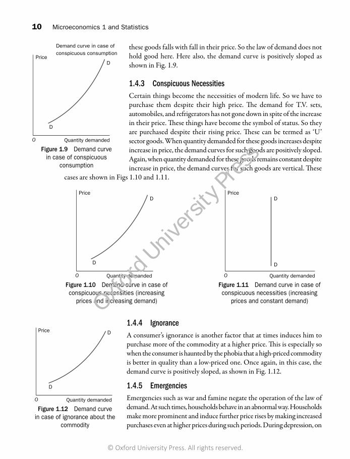
1.4.2 Conspicuous ConsumptionThis exception to the law of demand is associated with the doctrine propounded by Thorsten Veblen. A few goods like diamonds, are purchased by the rich and wealthy sections of the society. The prices of these goods are so high that they are beyond the reach of the common man. The higher the price of the diamond, the higher the prestige value of it. So when price of these goods falls, the consumers think that the prestige value of these goods comes down. So quantity demanded of
P1
Price
Quantity demandedO Q1 Q2
DD1
BA
DD1
Figure 1.6 Shifting of demand curve due to increase in the price
of substitute good
P1
Price
Quantity demandedO Q2 Q1
D1
D
AB
D1
D
Figure 1.7 Shifting of demand curve due to increase in the price
of complement good
Price
Quantity demandedO
D
D
Figure 1.8 Demand curve in case of Giffen good
Microeconomics.indb 9 6/21/2017 6:43:26 PM
© Oxford University Press. All rights reserved.
Oxford
Universi
ty Pre
ss
10 Microeconomics 1 and Statistics
Price
Quantity demandedO
D
D
Figure 1.12 Demand curve in case of ignorance about the
commodity
these goods falls with fall in their price. So the law of demand does not hold good here. Here also, the demand curve is positively sloped as shown in Fig. 1.9.
1.4.3 Conspicuous NecessitiesCertain things become the necessities of modern life. So we have to purchase them despite their high price. The demand for T.V. sets, automobiles, and refrigerators has not gone down in spite of the increase in their price. These things have become the symbol of status. So they are purchased despite their rising price. These can be termed as ‘U’ sector goods. When quantity demanded for these goods increases despite increase in price, the demand curves for such goods are positively sloped. Again, when quantity demanded for these goods remains constant despite increase in price, the demand curves for such goods are vertical. These
cases are shown in Figs 1.10 and 1.11.
Price
Quantity demandedO
D
Demand curve in case of conspicuous consumption
D
Figure 1.9 Demand curve in case of conspicuous
consumption
Price
Quantity demandedO
D
D
Figure 1.10 Demand curve in case of conspicuous necessities (increasing
prices and increasing demand)
Figure 1.11 Demand curve in case of conspicuous necessities (increasing
prices and constant demand)
Price
Quantity demandedO
D
D
1.4.4 IgnoranceA consumer’s ignorance is another factor that at times induces him to purchase more of the commodity at a higher price. This is especially so when the consumer is haunted by the phobia that a high-priced commodity is better in quality than a low-priced one. Once again, in this case, the demand curve is positively sloped, as shown in Fig. 1.12.
1.4.5 EmergenciesEmergencies such as war and famine negate the operation of the law of demand. At such times, households behave in an abnormal way. Households make more prominent and induce further price rises by making increased purchases even at higher prices during such periods. During depression, on
Microeconomics.indb 10 6/21/2017 6:43:26 PM
© Oxford University Press. All rights reserved.
Oxford
Universi
ty Pre
ss
Basics of Demand 11
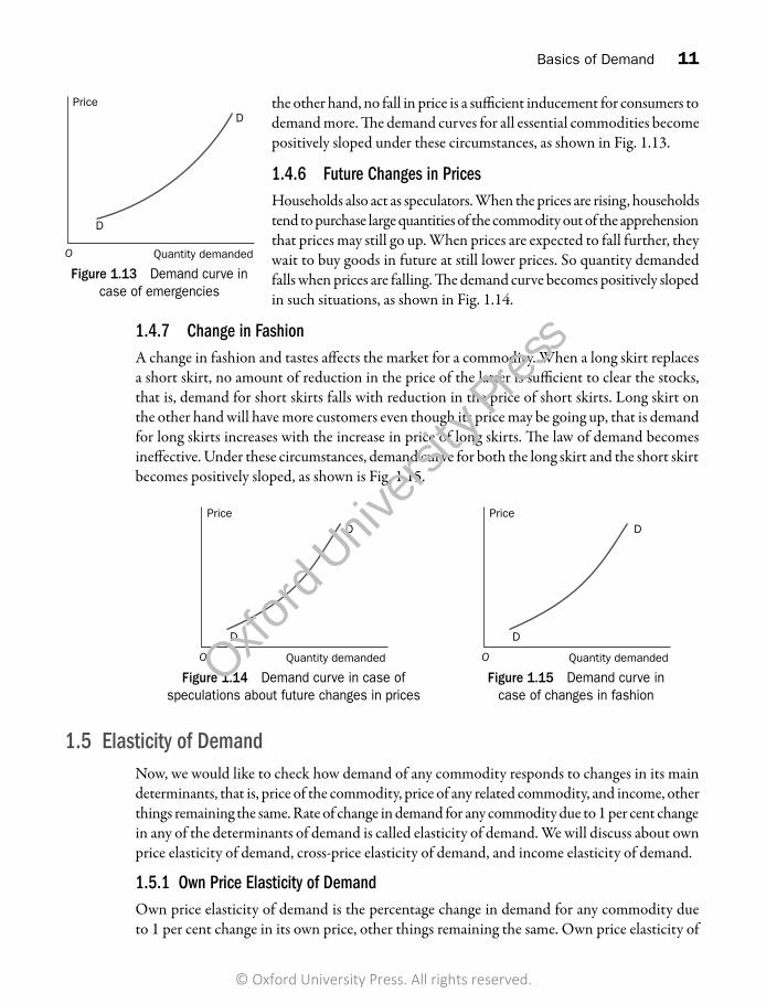
the other hand, no fall in price is a sufficient inducement for consumers to demand more. The demand curves for all essential commodities become positively sloped under these circumstances, as shown in Fig. 1.13.
1.4.6 Future Changes in PricesHouseholds also act as speculators. When the prices are rising, households tend to purchase large quantities of the commodity out of the apprehension that prices may still go up. When prices are expected to fall further, they wait to buy goods in future at still lower prices. So quantity demanded falls when prices are falling. The demand curve becomes positively sloped in such situations, as shown in Fig. 1.14.
1.4.7 Change in FashionA change in fashion and tastes affects the market for a commodity. When a long skirt replaces a short skirt, no amount of reduction in the price of the latter is sufficient to clear the stocks, that is, demand for short skirts falls with reduction in the price of short skirts. Long skirt on the other hand will have more customers even though its price may be going up, that is demand for long skirts increases with the increase in price of long skirts. The law of demand becomes ineffective. Under these circumstances, demand curve for both the long skirt and the short skirt becomes positively sloped, as shown is Fig. 1.15.
Price
Quantity demandedO
D
D
Figure 1.13 Demand curve in case of emergencies
Price
Quantity demandedO
D
D
Figure 1.14 Demand curve in case of speculations about future changes in prices
Price
Quantity demandedO
D
D
Figure 1.15 Demand curve in case of changes in fashion
1.5 Elasticity of DemandNow, we would like to check how demand of any commodity responds to changes in its main determinants, that is, price of the commodity, price of any related commodity, and income, other things remaining the same. Rate of change in demand for any commodity due to 1 per cent change in any of the determinants of demand is called elasticity of demand. We will discuss about own price elasticity of demand, cross-price elasticity of demand, and income elasticity of demand.
1.5.1 Own Price Elasticity of DemandOwn price elasticity of demand is the percentage change in demand for any commodity due to 1 per cent change in its own price, other things remaining the same. Own price elasticity of
Microeconomics.indb 11 6/21/2017 6:43:26 PM
© Oxford University Press. All rights reserved.
Oxford
Universi
ty Pre
ss
12 Microeconomics 1 and Statistics
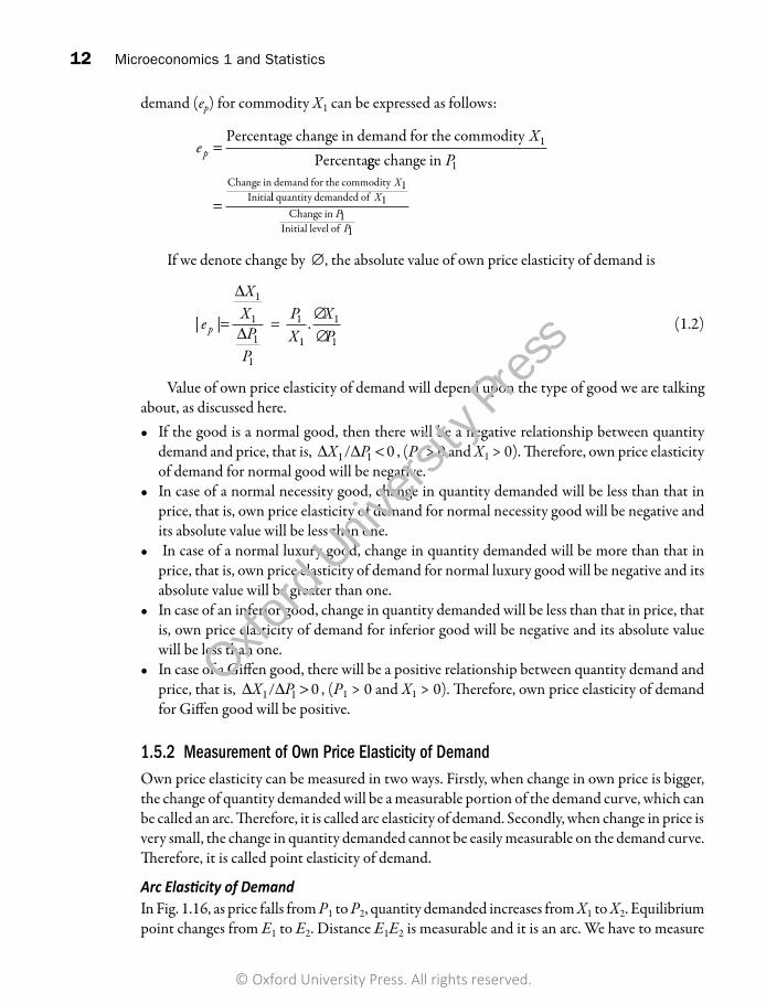
demand (ep) for commodity X1 can be expressed as follows:
eX
p =Percentage change in demand for the commodity
Percenta1
gge change in 1Change in demand for the commodity 1
Initia
PX
= ll quantity demanded of 1Change in 1
Initial level of 1
XP
P
If we denote change by ∅, the absolute value of own price elasticity of demand is
| |e
XX
PP
p =
∆
∆
1
1
1
1
= PX
XP
1
1
1
1.∅∅
(1.2)
Value of own price elasticity of demand will depend upon the type of good we are talking about, as discussed here. • Ifthegoodisanormalgood,thentherewillbeanegativerelationshipbetweenquantity
demand and price, that is, ∆ ∆X P1 1 0/ < , (P1 > 0 and X1 > 0). Therefore, own price elasticity of demand for normal good will be negative.
• Incaseofanormalnecessitygood,changeinquantitydemandedwillbelessthanthatinprice, that is, own price elasticity of demand for normal necessity good will be negative and its absolute value will be less than one.
• Incaseofanormalluxurygood,changeinquantitydemandedwillbemorethanthatinprice, that is, own price elasticity of demand for normal luxury good will be negative and its absolute value will be greater than one.
• Incaseofaninferiorgood,changeinquantitydemandedwillbelessthanthatinprice,thatis, own price elasticity of demand for inferior good will be negative and its absolute value will be less than one.
• IncaseofaGiffengood,therewillbeapositiverelationshipbetweenquantitydemandandprice, that is, ∆ ∆X P1 1 0/ > , (P1 > 0 and X1 > 0). Therefore, own price elasticity of demand for Giffen good will be positive.
1.5.2 Measurement of Own Price Elasticity of DemandOwn price elasticity can be measured in two ways. Firstly, when change in own price is bigger, the change of quantity demanded will be a measurable portion of the demand curve, which can be called an arc. Therefore, it is called arc elasticity of demand. Secondly, when change in price is very small, the change in quantity demanded cannot be easily measurable on the demand curve. Therefore, it is called point elasticity of demand.
Arc Elasticity of DemandIn Fig. 1.16, as price falls from P1 to P2, quantity demanded increases from X1 to X2. Equilibrium point changes from E1 to E2. Distance E1E2 is measurable and it is an arc. We have to measure
Microeconomics.indb 12 6/21/2017 6:43:30 PM
© Oxford University Press. All rights reserved.
Oxford
Universi
ty Pre
ss

Basics of Demand 13
elasticity on this arc. If we consider P1 the initial price and X1 the initial quantity demanded, change is price is P2 − P1 and change is quantity demanded is X2 − X1. Arc elasticity of demand is
Earc
Change in quantity demandedOriginal quantity demanded= CChange in own price
original own price
=
−
− =
X XX
P PP
PX
2 1
1
2 1
1
1
1⋅⋅ −
−X XP P
2 1
2 1
(1.3)
If we consider P2 the initial price and X2 the initial quantity demanded, change is price is P1 − P2 and change is quantity demanded is X1 − X2. Arc elasticity of demand is
Earc
Change in quantity demandedOriginal quantity demanded= CChange in own price
Original own price
X XX
P PP
PX
1 2
2
1 2
2
2
2
−
− = ⋅ XX XP P
1 2
1 2
−−
(1.4)
If we compare these two values of arc elasticity,
X XP P
X XP P
2 1
2 1
1 2
1 2
−−
= −−
However,
PX
PX
1
1
2
2↑
Therefore, if we measure the arc elasticity from two opposite side, values will be different. To solve this problem, we consider the average value of both price and quantity as initial price and quantity.
Therefore,
Earc=
X XX X
P PP P
X XX X
P PP P
P PX
1 2
1 2
1 2
1 2
1 2
1 2
1 2
1 2
1 2
1
2
2
22
−+
−+
= −+
⋅ +−
= +( )( ) ++
⋅ −−X
X XP P2
1 2
1 2
(1.5)
E1P1
P2
X1 X1
E2
0 Quantity of X
Price of X
DD
Fig. 1.16 Arc elasticity of demand
Microeconomics.indb 13 6/21/2017 6:43:35 PM
© Oxford University Press. All rights reserved.
Oxford
Universi
ty Pre
ss
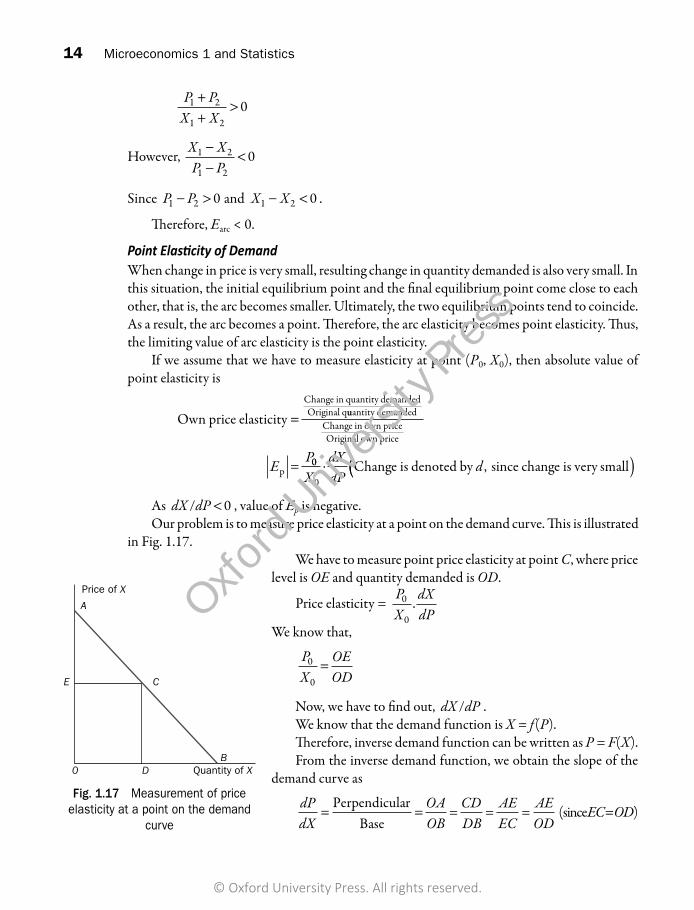
14 Microeconomics 1 and Statistics
P PX X
1 2
1 20
++
>
However, X XP P
1 2
1 20
−−
<
Since P P1 2 0− > and X X1 2 0− < .
Therefore, Earc < 0.
Point Elasticity of DemandWhen change in price is very small, resulting change in quantity demanded is also very small. In this situation, the initial equilibrium point and the final equilibrium point come close to each other, that is, the arc becomes smaller. Ultimately, the two equilibrium points tend to coincide. As a result, the arc becomes a point. Therefore, the arc elasticity becomes point elasticity. Thus, the limiting value of arc elasticity is the point elasticity.
If we assume that we have to measure elasticity at point (P0, X0), then absolute value of point elasticity is
Own price elasticityChange in quantity demandedOriginal q= uuantity demanded
Change in own priceOriginal own price
pE P= 00
0XdXdP
d⋅ Change is denoted by since change is very small,(( )As dX dP/ < 0 , value of Ep is negative.Our problem is to measure price elasticity at a point on the demand curve. This is illustrated
in Fig. 1.17.We have to measure point price elasticity at point C, where price
level is OE and quantity demanded is OD.
Price elasticity = PX
dXdP
0
0.
We know that,
PX
OEOD
0
0=
Now, we have to find out, dX dP/ .We know that the demand function is X = f(P).Therefore, inverse demand function can be written as P = F(X).From the inverse demand function, we obtain the slope of the
demand curve as
dPdX
OAOB
= CDDB
= AEEC
= AEOD
= =PerpendicularBase
(since EC = OD)
0 Quantity of X
Price of X
CE
A
BD
Fig. 1.17 Measurement of price elasticity at a point on the demand
curve
Microeconomics.indb 14 6/21/2017 6:43:41 PM
© Oxford University Press. All rights reserved.
Oxford
Universi
ty Pre
ss

Basics of Demand 15
Therefore,
Point price elasticity at point C = OEOD
ODAE
OEAE
BDOD
BCAC
. = = =
If point C is the mid-point of the demand curve, BC = AC. Therefore, Ep = 1.If the point lies on the upper half of the demand curve, BC > AC, therefore, Ep > 1.If the point lies on the lower half of the demand curve, BC < AC, therefore, Ep < 1.Point price elasticity at point A is ∞, since denominator = 0.Point price elasticity at point B is 0, since numerator = 0.
1.5.3 Elastic and Inelastic DemandThe shape of any demand curve depends upon the absolute value of elasticity of demand. The shapes of different demand curves according to the absolute values of elasticity of demand are explained as follows:• Whenpriceelasticityofdemandislessthanone,itiscalledinelasticdemand,asincaseof
necessity goods. Such a demand curve is shown in Fig. 1.18.• Whenpriceelasticityofdemandismorethanone,itiscalledelasticdemand,asincaseof
luxury goods. Such a demand curve is shown in Fig. 1.19.
0 Quantity
Price
P1
P2
Q1 Q2
D
D
Fig. 1.18 Inelastic demand curve
0 Quantity
Price
P1
P2
Q1 Q2
D
D
Fig. 1.19 Elastic demand curve
• Whenpriceelasticityofdemandisequaltoone,itiscalledunitaryelasticdemand.Suchademand curve is shown in Fig. 1.20.
• Whenpriceelasticityofdemand isequal to∞, it iscalledperfectlyelasticdemand.Theshape of a perfectly elastic demand curve is horizontal. Such a demand curve is shown inFig. 1.21.
• Whenpriceelasticityofdemandisequalto0,itiscalledperfectlyinelasticdemand.Theshape of a perfectly inelastic demand curve is vertical. Such a demand curve is shown inFig. 1.22.
Microeconomics.indb 15 6/21/2017 6:43:42 PM
© Oxford University Press. All rights reserved.
Oxford
Universi
ty Pre
ss

16 Microeconomics 1 and Statistics
0
Quantity of X
D
A1
Price of X
C C1
B B1
A
Fig. 1.23 Demand curves with same slope but different elasticities
of demand
1.5.4 Distinction between Slope of a Demand Curve and Elasticity of DemandSlope of the demand curve and elasticity of demand are two different concepts.
Inverse demand function is P = F(X). From this inverse demand function, we get the slope of the demand curve as dP dX/ .
On the other hand, price elasticity of demand is
PX
dXdP⋅ or
PX
dPdX
Therefore, we can say that elasticity of demand and slope of the demand curve are not the same.
We can show that, • Twodemandcurvescanhavethesameslopebuttheirelasticities
can be different.• Two demand curves can have different slopes but their
elasticities can be same.• Thehighertheslopeofthedemandcurve,thelowerwillbethe
elasticity and vice versa. It can be shown that two demand curves can have the same slope,
but elasticities of demand can be different. In Fig. 1.23, two demand curves AB and A1B1 are parallel to each
other. For price level OD, we have equilibrium point C on AB and equivalent equilibrium point C1 on A1B1. Since two demand curves AB and A1B1 are parallel to each other,
OAOB
OAOB
= 1
1
Fig. 1.20 Unitary elastic demand curve
0 Quantity
Price
P1
P2
Q1 Q2
D
D
0 Quantity
Price
P DD
Fig. 1.21 Perfectly elastic demand curve
Fig. 1.22 Perfectly inelastic demand curve
0 Quantity
Price
D
D
Q0
Microeconomics.indb 16 6/21/2017 6:43:46 PM
© Oxford University Press. All rights reserved.
Oxford
Universi
ty Pre
ss

Basics of Demand 17
Therefore, AB and A1B1 have the same slope.We have to find out the elasticity of demand for these two demand curves at two equivalent
equilibrium points C and C1.
Elasticity of demand at C = BCCA
ODDA
=
Elasticity of demand at C1= B CC A
ODDA
1 1
1 1 1=
Since, DA1 > DA,
ODDA
ODDA1
<
Therefore, elasticity of demand of AB at point C is greater than that of A1B1 at point C1.It can also be shown that two demand curves can have the same elasticity of demand, but
their slopes can be different. In the first part of Fig. 1.24, we have two demand curves AB and AC with same vertical
intercept. If we try to measure elasticity of demand on two equivalent points H and I, we see that
At point H, elasticity of demand is BHHA
OGGA
=
Again,
Elasticity of demand at point I is CIIA
OGGA
=
Therefore, elasticity of demand at point H is the same as elasticity of demand at point I.
Price of X Price of X
A
G
0
H I
B C 0
Quantity of X Quantity of X
D
D1J
K
L
E
Fig. 1.24 Two demand curves with same elasticity of demand, but different slopes
Microeconomics.indb 17 6/21/2017 6:43:49 PM
© Oxford University Press. All rights reserved.
Oxford
Universi
ty Pre
ss
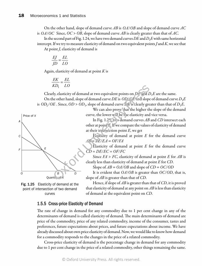
18 Microeconomics 1 and Statistics
On the other hand, slope of demand curve AB is OA OB/ and slope of demand curve AC is OA OC/ Since, OC > OB, slope of demand curve AB is clearly greater than that of AC.
In the second part of Fig. 1.24, we have two demand curves DE and D1E with same horizontal intercept. If we try to measure elasticity of demand on two equivalent points J and K, we see that
At point J, elasticity of demand is
EJJD
ELLO
=
Again, elasticity of demand at point K is
EKKD
ELLO1
=
Clearly, elasticity of demand at two equivalent points on DE and D1E are the same.On the other hand, slope of demand curve DE is OD OE/ and slope of demand curve D1E
is OD OE1/ . Since, OD > OD1, slope of demand curve DE is clearly greater than that of D1E. We can also prove that the higher the slope of the demand
curve, the lower will be the elasticity and vice versa.In Fig. 1.25, two demand curves AB and CD intersect each
other at point E. If we compare the values of elasticity of demand at their intersection point E, we get
Elasticity of demand at point E for the demand curve AB = BE/EA = OF/FA
Elasticity of demand at point E for the demand curve CD = DE/EC = OF/FC
Since FA > FC, elasticity of demand at point E for AB is clearly less than elasticity of demand at point E for CD.
Slope of AB = OA/OB and slope of CD = OC/ODIt is evident that OA/OB is greater than OC/OD, that is,
slope of AB is greater than that of CD.Hence, if slope of AB is greater than that of CD, it is proved
that elasticity of demand at any point on AB is less than elasticity of demand at the equivalent point on CD.
1.5.5 Cross-price Elasticity of DemandThe rate of change in demand for any commodity due to 1 per cent change in any of the determinants of demand is called elasticity of demand. The main determinants of demand are price of the commodity, price of any related commodity, income of the consumer, tastes and preferences, future expectations about prices, and future expectations about income. We have already discussed about own price elasticity of demand. Now, we would like to know how demand for a commodity responds to the changes in the price of a related commodity.
Cross-price elasticity of demand is the percentage change in demand for any commodity due to 1 per cent change in the price of a related commodity, other things remaining the same.
A
C
F E
O B D
Price of X
Quantity of X
Fig. 1.25 Elasticity of demand at the point of intersection of two demand
curves
Microeconomics.indb 18 6/21/2017 6:43:53 PM
© Oxford University Press. All rights reserved.
Oxford
Universi
ty Pre
ss

Basics of Demand 19
Cross-price elasticity of demand (ec1) for commodity X1 can be expressed as follows:
eX
c1 =Percentage change in demand for the commodity
Percent1
aage change in 2Change in demand for the commodity 1
Initi
PX
= aal quantity demanded of 1Change in 2
Initial level of 2
XP
P
If we denote change by ∅, we can write
e
XXP
P
PX
XPc1
1
1
2
2
2
1
1
2= =
∆
∆∆∆
. (1.6)
Both P2 and X1 are positive. Therefore, sign of cross elasticity of demand for X1 will depend on ∅∅
XP
1
2. Again, sign of
∅∅
XP
1
2will depend upon the nature of relationship between the commodities
X1 and X2. As price of X2, that is, P2, increases, demand for X2 decreases.• IfthetwocommoditiesX1 and X2 are substitutes to each other, as demand for X2 decreases,
demand for X1 increases. In short, as P2 increases, demand for X1 increases and vice versa.Therefore, the sign of cross elasticity of demand for X1, that is, ec1, is positive.
• If the two commodities X1 and X2 are complements to each other, as demand for X2
decreases, demand for X1 also decreases. In short, as P2 increases, demand for X1 decreasesand vice versa. Therefore, the sign of cross elasticity of demand for X1, that is, ec1, isnegative.
• If the two commodities are completely unrelated to each other, as demand for X2
decreases, there is no change in demand for X1. In short, as P2 increases or decreases,demand for X1 does not change at all. Therefore, cross elasticity of demand for X1, thatis, ec1, is zero.
1.5.6 Income Elasticity of DemandWe have already discussed about own price elasticity of demand and cross-price elasticity of demand. Now we would like to know how demand for a commodity responds to the changes in the income of the consumer.
Income elasticity of demand is the percentage change in demand for any commodity due to 1 per cent change in the income (M) of the consumer, other things remaining the same.
Income elasticity of demand (em) for commodity X1 can be expressed as follows:
eX
m =Percentage change in demand for the commodity
Percenta1
gge change in incomeChange in demand for the commodity 1
MX
= IInitial quantity demanded of 1Change in
Initial level of
XM
M
Microeconomics.indb 19 6/21/2017 6:43:57 PM
© Oxford University Press. All rights reserved.
Oxford
Universi
ty Pre
ss
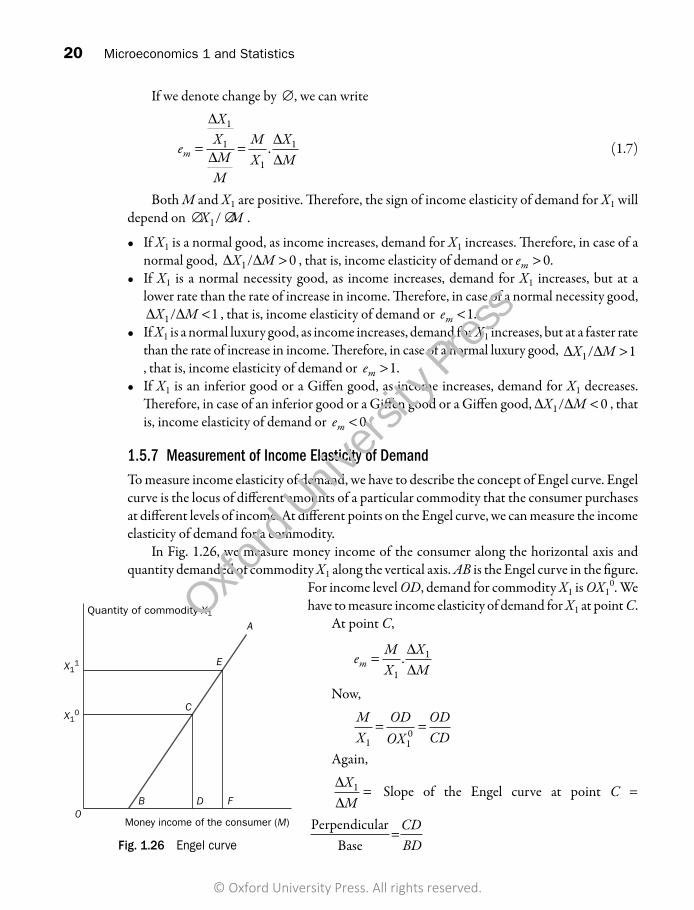
20 Microeconomics 1 and Statistics
If we denote change by ∅, we can write
e
XXM
M
MX
XMm = =
∆
∆∆∆
1
1
1
1. (1.7)
Both M and X1 are positive. Therefore, the sign of income elasticity of demand for X1 will depend on ∅ ∅X M1/ .
• IfX1 is a normal good, as income increases, demand for X1 increases. Therefore, in case of a normal good, ∆ ∆X M1 0/ > , that is, income elasticity of demand or em > 0.
• IfX1 is a normal necessity good, as income increases, demand for X1 increases, but at a lower rate than the rate of increase in income. Therefore, in case of a normal necessity good, ∆ ∆X M1 1/ < , that is, income elasticity of demand or em <1.
• IfX1 is a normal luxury good, as income increases, demand for X1 increases, but at a faster rate than the rate of increase in income. Therefore, in case of a normal luxury good, ∆ ∆X M1 1/ >, that is, income elasticity of demand or em >1.
• IfX1 is an inferior good or a Giffen good, as income increases, demand for X1 decreases. Therefore, in case of an inferior good or a Giffen good or a Giffen good, ∆ ∆X M1 0/ < , that is, income elasticity of demand or em < 0.
1.5.7 Measurement of Income Elasticity of DemandTo measure income elasticity of demand, we have to describe the concept of Engel curve. Engel curve is the locus of different amounts of a particular commodity that the consumer purchases at different levels of income. At different points on the Engel curve, we can measure the income elasticity of demand for a commodity.
In Fig. 1.26, we measure money income of the consumer along the horizontal axis and quantity demanded of commodity X1 along the vertical axis. AB is the Engel curve in the figure.
For income level OD, demand for commodity X1 is OX10. We
have to measure income elasticity of demand for X1 at point C.At point C,
e MX
XMm =
1
1.∆∆
Now,
MX
ODOX
ODCD1 1
0= =
Again,
∆∆
XM
1 = Slope of the Engel curve at point C =
PerpendicularBase
=CDBD
Quantity of commodity X1
Money income of the consumer (M)
C
0DB
E
A
F
X11
X10
Fig. 1.26 Engel curve
Microeconomics.indb 20 6/21/2017 6:44:06 PM
© Oxford University Press. All rights reserved.
Oxford
Universi
ty Pre
ss

Basics of Demand 21
Quantity of commodity X1
Money income of the consumer (M)
AE
D
C
B 0 F G
Fig. 1.28 Engel curve with negative intercept
Therefore, at point C,
e MX
XM
ODCD
CDBD
ODBDm = =
1
1.∆∆
. =
Similarly, at point E,
e MX
XM
OFEF
EFBF
OFBFm = =
1
1.∆∆
. =
The Engel curve AB is positively sloped. Therefore, it is clear that as income increases, consumer demand for X1 increases. Therefore, em is positive. Moreover, since, Engel curve AB has a positive intercept in the horizontal axis, that is, when income is OB, the demand for commodity X1 is zero, OD > BD, and also OF > BF. Therefore, em is always greater than one for commodity X1.
In Fig. 1.27, Engel curve OA has zero intercept in the horizontal axis, that is, it passes through the origin. In other words, when income is zero, demand for commodity X1 is also zero. Under these circumstances,
MX
ODBD1
= and ∆∆
XM
BDOD
1 =
Therefore, at point B,
e MX
XM
ODBD
BDODm = = =
1
1 1. .∆∆
Similarly, at point C or at any other point on the Engel curve OA, em = 1.In Fig. 1.28, Engel curve AB has a negative intercept in the horizontal axis, that is, when
income is zero, the demand for commodity X1 is OC, that is, positive. Therefore, at point D,
e OFBFm = <1
In addition, at point E,
e OGBGm = <1
Similarly, at any other point on the Engel curve AB, em < 1.In Fig. 1.29, Engel curve AB is an upward rising curve. To
measure income elasticity of demand for X1, at any point, say E, on the curve AB, we have to draw a tangent of the curve through point E. Slope of the curve AB at point E is the slope of the tangent CD at point E, that is, Price of X Price of X
A
G
0
H I
B C 0
Quantity of X Quantity of X
D
D1J
K
L
E
.
Quantity of commodity X1
Money income of the consumer (M)
B
O D
C
A
E
Fig. 1.27 Engel curve with zero intercept
Microeconomics.indb 21 6/21/2017 6:44:11 PM
© Oxford University Press. All rights reserved.
Oxford
Universi
ty Pre
ss

22 Microeconomics 1 and Statistics
Therefore, at point E,
e MX
XM
OFEF
EFDF
OFDFm = = =
1
1. .∆∆
If the commodity X1 is an inferior good, then as income increases, demand for commodity X1 decreases. Therefore, Engel curve for commodity X1 will slope negatively as shown in Fig. 1.30. In Fig. 1.30, the Engel curve AB is a negatively sloped straight line. At point C,
MX
ODCD1
= and ∆∆
XM
CDDB
1 = −
Therefore, at point C,
e MX
XM
ODCD
CDDB
ODDBm = = − = −
1
1. .∆∆
Hence, at any other point on the Engel curve AB, em < 0.
Money income of the consumer (M)
Quantity of commodity X1
D0 F
A
E
B
C
Fig. 1.29 Upward rising Engel curve
Money income of the consumer (M)
Quantity of commodity X1
D0
A
B
C
Fig. 1.30 Downward or negative slope of Engel curve
SUMMARY
• Demand is a consumer’s readiness and capability topay a price for a specific quantity of a good or serviceat a given point of time. The relationship betweenprice and quantity demanded is known as the demand relationship. The law of demand states that the quantity demanded and the price of a commodity are inversely related, other things remaining constant. All the goods, for which law of demand is applicable, are called normal goods.
• Demand for certain good or service depends on anumber of different factors, for example, personal
disposable income of the consumer, prices of the related goods and services, preferences of the consumer, and expectations about the future prices and income.
• Demand function is the behavioural relationshipbetween quantity demanded for a good or serviceand all the factors that influence the demand for thatgood or service.
• A demand schedule lists prices and correspondingquantities based on law of demand. We can construct the demand curve of an individual based on the demand
Microeconomics.indb 22 6/21/2017 6:44:14 PM
© Oxford University Press. All rights reserved.
Oxford
Universi
ty Pre
ss
Basics of Demand 23
SHORT-ANSWER TYPE QUESTIONS (2 MARKS)
1. What do you mean by demand?2. What is law of demand?3. State the law of demand. Mention any two exceptions to
this law. [CU B Com (G), 2012]4. What do you mean by a normal good?5. Mention the factors determining demand.6. What is the relation between demand for a good and its
own price?7. What is the relation between demand for a good and the
price of its substitute?
8. What is the relation between demand for a good and the price of its complement?
9. What is the relation between demand for a good and the income of the consumer?
10. What is the relation between demand for a good and the tastes and preferences of the consumers?
11. What is the relation between demand for a good and future expectations of the consumer about the price of the good?
E X E R C I S E S
[According to CU syllabus of Economic-I paper for B Com Honours and General, second unit requires three lectures and four marks. Therefore, we have incorporated the short-answer type questions carrying two marks and medium-answer type questions carrying four
marks in the exercise.]
schedule. Demand curve is the locus of all the price–quantity combinations which follow the law of demand. Since the demand curve follows the law of demand, it is negatively sloped.
• Individual demand curves differ from person toperson in their slopes and shapes. We can sum upall individual demand curves and derive a marketdemand curve.
• Movement along the demand curve occurs whenthere is a change in the own price. There are variousdeterminants of demand for a commodity apart fromits price, for example, personal disposable incomeof the consumer, prices of the related goods andservices, preferences of the consumer, etc. A shiftin the demand curve occurs when any one of thosedeterminants change.
• The circumstances when the law of demand becomes ineffective are known as exceptions of the law ofdemand. In those cases, the demand curve doesnot follow the law of demand and therefore it is notdownward sloping.
• The rate of change in demand for any commodity dueto 1 per cent change in any of the determinants ofdemand is called elasticity of demand.
• Own price elasticity of demand is the percentagechange in demand for any commodity due to 1 per
cent change in its own price, other things remaining the same.
• Own price elasticity can be measured in two ways.Firstly, when change in own price is bigger, thechange of quantity demanded will be a measurableportion of the demand curve, which can be called anarc. Therefore, it is called arc elasticity of demand.Secondly, when change in price is very small, thechange in quantity demanded cannot be easilymeasurable on the demand curve. Therefore, it iscalled point elasticity of demand.
• The elasticity of demand and slope of the demandcurve are not same.
• The cross-price elasticity of demand is the percentage change in demand for any commodity due to 1 percent change in the price of a related commodity, otherthings remaining the same.
• Income elasticity of demand is the percentage changein demand for any commodity due to 1 per cent change in the income of the consumer, other things remaining the same.
• Engel curve is the locus of different amounts of aparticular commodity that the consumer purchases atdifferent levels of income. At different points on theEngel curve, we can measure the income elasticityof demand for a commodity.
Microeconomics.indb 23 6/21/2017 6:44:14 PM
© Oxford University Press. All rights reserved.
Oxford
Universi
ty Pre
ss
24 Microeconomics 1 and Statistics
12. What is the relation between demand for a good and the future expectations of the consumer about his/her income?
13. What is meant by a demand function?[CU B Com (G), 2005]
14. State the demand function in its general form. 15. What do you mean by a demand schedule? 16. What is the shape of the demand curve for a normal good? 17. What is market demand? 18. How can market demand be derived from individual
demand? [CU B Com (G), 2012] 19. Under what circumstances does the demand curve shift?
[CU B Com (G), 2005] 20. How will the demand curve change with the increase in
income of the consumer? [CU B Com (G), 2005] 21. Mention two cases where the consumer demand curve
shifts upwards. [CU B Com (G), 2009] 22. What is the shape of the demand curve in case of Giffen
goods? 23. What is the shape of the demand curve in case of
conspicuous consumption? 24. What is the shape of the demand curve in case of
conspicuous necessities? 25. What is the shape of the demand curve in case of
ignorance of the consumers? 26. What is the shape of the demand curve in case of
emergencies? 27. What is the shape of the demand curve in case of a future
expectation of price rise? 28. What is the shape of the demand curve in case of a future
expectation of fall in price? 29. What is the shape of the demand curve in case of a
change in fashion? 30. What do you mean by elasticity of demand? 31. What do you mean by price elasticity of demand?
[CU B Com (G), 2009] 32. What is own price elasticity of demand? 33. What is the difference between arc elasticity of demand
and point elasticity of demand? 34. What will be the value of own price elasticity of demand
for a normal good? 35. What will be the value of own price elasticity of demand
for a normal necessity good? 36. What will be the value of own price elasticity of demand
for a normal luxury good?
37. What will be the value of own price elasticity of demand for an inferior good?
38. What will be the value of own price elasticity of demand for a Giffen good?
39. What is elastic demand? 40. What is inelastic demand? 41. What is the shape of a perfectly elastic demand curve? 42. What is the shape of a perfectly inelastic demand curve? 43. At which point on a downward sloping straight line
demand curve the absolute value of the price-elasticity of demand is unity? [CU B Com (G), 2007]
44. What is meant by ‘cross-price elasticity of demand’? [CU B Com (G), 2010]
45. If the cross-price elasticity of two related goods is positive, what is the relationship between the aforesaid goods? [CU B Com (G), 2008]
46. If the cross-price elasticity of two related goods negative, what is the relationship between the aforesaid goods?
47. If the cross-price elasticity of two goods is zero, what is the relationship between the aforesaid goods?
48. What do you mean by income elasticity of demand? 49. What will be the value of income elasticity of demand for
a normal good? 50. What will be the value of income elasticity of demand for
a normal necessity good? 51. What will be the value of income elasticity of demand for
a normal luxury good? 52. What will be the value of income elasticity of demand for
an inferior good? 53. What will be the value of income elasticity of demand for
a Giffen good? 54. What is an Engel curve? 55. If the Engel curve is upward rising with a positive
intercept on the horizontal axis, what will be value of income elasticity of demand at any point on the curve?
56. If the Engel curve is upward rising with a negativeintercept on the horizontal axis, what will be valueof income elasticity of demand at any point on the curve?
57. If the Engel curve is upward rising passing through the origin, what will be value of income elasticity of demand at any point on the curve?
Microeconomics.indb 24 6/21/2017 6:44:14 PM
© Oxford University Press. All rights reserved.
Oxford
Universi
ty Pre
ss

Basics of Demand 25
MEDIUM-ANSWER TYPE QUESTIONS (4 MARKS)
1. What is law of demand? Why does a demand curve have negative slope? [CU B Com (G), 2006]
2. Draw and explain separately an individual demand curve and market demand curve for a normal good.
[CU B Com (G), 2005, 2012]3. How is market demand curve determined from an
individual demand curve? [CU B Com (G), 2005, 2012]
4. The demand schedule of pulses for a consumer is given in Table 1.3. Derive the individual demand curve for pulses from the demand schedule.
Table 1.3 Demand schedule of pulses for a consumer
Price per kg. (`) Quantity demanded (in kg)
50 1
40 2
30 3
20 4
10 5
5. For what reasons does a demand curve shift? Explain diagrammatically the difference between the change in demand and change in quantity demanded?
[CU B Com (G), 2007, 2011]6. The demand schedule of pulses for two consumers is
given in Table 1.4. Fill up the blanks for market demand in the schedule and derive the market demand curve for pulses from the demand schedule assuming that there are only two consumers in the whole market.
7. State the law of demand. Mention two exceptions to this law. Explain the factors affecting demand.
[CU B Com (G), 2009]
8. Mention two exceptions to the law of demand. Explain the factors affecting demand. [CU B Com (G), 2012]
9. Distinguish between ‘change in demand’ and ‘change in quantity demanded’.
10. What do you mean by arc elasticity of demand? How can you measure own price elasticity of demand on an arc of a straight line demand curve?
11. How can you measure point price elasticity of demand on any point of a straight line demand curve?
12. Prove that on a straight line demand curve, value of point price elasticity of demand will be unity at the mid-point of the demand curve.
13. Explain the difference between slope of a demand curve and elasticity of demand.
14. Explain the concepts of income elasticity of demand and cross-price elasticity of demand. [CU B Com (G), 2011]
15. Define cross-price elasticity of demand. How are the concerned goods related to each other if the cross-price elasticity is positive? [CU B Com (G), 2012]
16. How can you measure income elasticity of demand?
LONG-ANSWER TYPE QUESTIONS (8 MARKS)
1. What is price elasticity of demand? On what factors does it depend? [CU B Com (G), 2007]
2. What is price elasticity of demand? How can the price elasticity of demand be measured at a point on a downward sloping straight line demand curve?
[CU B Com (G), 2008]
3. Show that on a linear demand curve, the absolute value of elasticity of demand varies between zero and infinity.
4. What is the relation between slope of a demand curve and elasticity of demand? Show that two demand curves can have same slope but different elasticities of demand
Table 1.4 Demand schedule of pulses for two consumers
Price per kg.
(`)
Quantity demanded
by consumer 1 (in kg)
Quantity demanded
by consumer 2 (in kg)
Market demand of pulses
50 1 0
40 2 1
30 3 2
20 4 3
10 5 4
Microeconomics.indb 25 6/21/2017 6:44:14 PM
© Oxford University Press. All rights reserved.
Oxford
Universi
ty Pre
ss

26 Microeconomics 1 and Statistics
and two demand curves can have same elasticity of demand but different slope.
5. Define the concepts of the following:• Incomeelasticityofdemand• Cross-priceelasticityofdemand
[CU B Com (G), 2009]6. What do you mean by cross-price elasticity of
demand? Show that the value of cross-price elasticity
of demand depends on the relation between the concerned goods.
7. What do you mean by elasticity of supply? How can you measure elasticity of supply at any point on the supply curve?
8. What do you mean by elastic and inelastic supply? Show how shapes of the supply curve will be different for different values of elasticity of supply.
Microeconomics.indb 26 6/21/2017 6:44:14 PM
© Oxford University Press. All rights reserved.
Oxford
Universi
ty Pre
ss