metropolitan land values - david albouydavidalbouy.net/landvalue_index.pdf · metropolitan land...

Metropolitan Land Values∗

David Albouy

University of Illinois and NBER

Gabriel Ehrlich

University of Michigan

Minchul Shin

University of Illinois

June 11, 2017

∗We would like to thank Henry Munneke, Nancy Wallace, and participants at seminars at the AREUEAAnnual Meetings (Chicago), Ben-Gurion University, Brown University, the Federal Reserve Bank of NewYork, the Housing-Urban-Labor-Macro Conference (Atlanta), Hunter College, the NBER Public EconomicsProgram Meeting, the New York University Furman Center, the University of British Columbia, the Uni-versity of California, the University of Connecticut, the the University of Georgia, the University of Illinois,the University of Michigan, the University of Rochester, the University of Toronto, the Urban EconomicsAssociation Annual Meetings (Denver), and Western Michigan University for their help and advice. Weespecially want to thank Morris Davis, Andrew Haughwout, and Matthew Turner for sharing data, or in-formation about data, with us. We thank Nicolas Bottan for outstanding research assistance. The NationalScience Foundation (Grant SES-0922340) generously provided financial assistance. Please contact the au-thors by e-mail at [email protected] or by mail at University of Illinois, Department of Economics, 1407W. Gregory, 18 David Kinley Hall, Urbana, IL 61801.

Abstract

We estimate the first cross-sectional index of transaction-based land values for every U.S. metropoli-tan area. The index accounts for geographic selection and incorporates novel shrinkage methodsusing a prior belief based on urban economic theory. Land values at the city center increase withcity size, as do land-value gradients; both are highly variable across cities. Urban land valuesare estimated at more than two times GDP in 2006. These estimates are higher and less volatilethan estimates from residual (total - structure) methods. Five urban agglomerations account for 48percent of all urban land value in the United States.

JEL Codes: C43, R1, R3Keywords: land values, monocentric city, hierarchical modeling

1 Introduction

We estimate the first index of directly-observed market values for land that is cross-sectionallycomparable across U.S. metropolitan areas. Standard economic theory, e.g. Roback (1982),Brueckner (1983), and Albouy (2016), suggests that this index captures differences in the privatevalue of household amenities, employment, and building opportunities combined across metro ar-eas. Urban land values have been central to questions of wealth, income, and taxation since theseminal works of Ricardo (1821) and George (1884).

Unfortunately, market data on land values have been notoriously piecemeal and subject tonumerous measurement challenges. Flow of Funds (FOF) accounts of the Federal Reserve stoppedpublishing series for land value in 1995 because of accuracy concerns made plain by negativevalues inferred for land. We aim to overcome these challenges using a large national data set ofmarket transactions of land from the CoStar COMPS database and an econometric model informedby urban theory. Our estimates of urban land values prove to be higher and more stable than valuesimplied by the FOF.

Our indexes of both central and average land values have intuitive properties. While they varyconsiderably, the indexes increase with city area, providing nuanced support for the monocentriccity model of Alonso (1964), Mills (1967), and Muth (1969). The highest central land valuesare found in New York, Chicago, Washington, San Francisco, and Los Angeles. In these cities,central values are 21 times higher than peripheral values 10 miles away, although across all citiesthe (unweighted) average ratio of central to peripheral values is only 4. Over their entire urbanareas, New York, Jersey City, Honolulu, San Francisco, and Los Angeles-Long Beach have thehighest average values, which are 82 times higher than those in the lowest five cities. Values in2009 averaged $373,000 per acre, down from $624,000 in 2006, as the total value of urban landfell from $28 to $18 trillion, or from 2.2 to 1.3 times GDP.

2 Description of Transactions Data and Urban Land Area

Our primary data source is the CoStar COMPS database, with land transaction prices recordedbetween 2005 and 2010.1 CoStar provides fields containing the price, lot size, address, and a

1The CoStar Group claims to have the commercial real estate industry’s largest research organization. The COMPSdatabase provided by CoStar University, free for academics, includes transaction details for all types of commercialreal estate. We use every sale CoStar considers “land.” Recently, a small literature has used this data for analyses withinmetro areas. Haughwout et al. (2008) demonstrate the data’s extensive coverage and construct a land price index for1999 to 2006 within the New York metro area. Kok et al. (2014) document land sales within the San Francisco BayArea, and relate sales prices to topographical, demographic, and regulatory features. Nichols et al. (2013) constructa panel of land-value indexes for 23 metros from the 1990s to 2009. These indexes are for use over time and are notcomparable across metros.

1

“proposed use” for each property. We exclude transactions CoStar has marked as non-arms length,without complete information, that feature a structure, are over 60 miles from the city center, orare less than $100 per acre. The remaining dataset contains 68,756 observed land sales.2

The “cities” we examine correspond to 1999 OMB definitions of Metropolitan Statistical Areas(MSAs). Some MSAs, known as Consolidated MSAs (CMSAs) are divided into constituent “Pri-mary” MSAs, which we treat as separate cities. In 2000, all MSAs accounted for 80 percent of theU.S. population. Because MSAs consist of counties, which often contain a large amount of agri-cultural land, we consider only land that is part of an urban area by 2000 Census definitions. Themain requirement is that the area consists of contiguous block groups with a population density ofover 1,000 residents per square mile (1.56 per acre), with a total population of over 2,500.

We take city centers to be the City Hall or Mayor’s office of each city. Many MSA namescontain multiple cities, e.g., Minneapolis-St. Paul. We address this by considering each namedcity as having its own center. Land parcels within the MSA are assigned to the city center closestin Euclidean distance. In such cases, our central values average the named centers.

Appendix Figure A.1 displays the geographic pattern of land sales for four CMSAs: NewYork, Los Angeles, Chicago, and Houston. The figure shows that land sales are well-dispersedthroughout the metro areas, with sales activity more frequent near city centers.3

3 Econometric Methods

There are two major obstacles to constructing a cross-metropolitan land value index from observedtransactions data. First, observed transactions are not a random sample of all parcels in a city.Second, we observe few sales in many smaller metro areas, reducing the reliability of the estimates.Our econometric methods try to overcome both of these obstacles.

2The appendix provides information on the treatment of the data as well as some descriptive statistics.3Land transactions are not randomly distributed over space. Yet, as Haughwout et al. (2008) comment on the New

York data, “Overall, vacant land transactions occurred throughout the region, with a heavy concentration in the mostdensely developed areas ...”. As Nichols et al. (2013) discuss, it is impossible to correct for all types of selection biaswithout observing transaction prices for unsold lots, a logical contradiction. Fortunately, the literature has generallyfound selection bias to be minor for land and commercial real estate prices. Colwell and Munneke (1997), studyingland prices in Cook County, IL, report, “The estimates with the selection variable and those without are surprisinglyconsistent for each land use.” Studying the office market in Phoenix, Munneke and Barrett (2000) find, “the priceindices generated after correcting for sample-selection bias do not appear significantly different from those that donot consider selectivity bias.” In their construction of metro price indices, Munneke and Barrett (2001) report, “Littleselection bias is found in the estimates.” Finally, Fisher et al. (2007), in their study of commercial real estate properties,state “sample selection bias does not appear to be an issue with our annual model specification.”

2

3.1 Regression Model of Land Values over Space and Time

Following the monocentric city model, we take each city j as having a fixed center, with co-ordinates zcj . Land values vary according to a city-specific polynomial in the distance metric,D(zij, z

cj), between plot i’s coordinates zij and the center, with coefficients δjk determining the

shape of the value-distance gradient:

ln rijt =2010∑t=2005

αjt +K∑k=1

δjk[D(zij, z

cj)]k

+Xijtβ + eijt, eijt ∼ i.i.d.N(0, σ2e). (1)

The specification allows for city-center values αjt to vary by year, t, and for controls Xijt, whichincludes proposed use and lot size.4

Figure 1a shows estimated first-order and fourth-order polynomials for the Houston MSA,along with the underlying transaction prices. Both polynomials generally slope downward withdistance, but the fourth-order polynomial allows for a richer distance function.

3.2 Shrinkage Estimation and Its Target

To deal with limited sample sizes we develop a hierarchical model, which “shrinks” estimatestowards national average functions. We allow the shrinkage target to depend on each city’s urbanarea, Aj . We begin by decomposing αjt into two parts, αjt = αj +α?jt, where α?j2005 is normalizedto zero. Vectorizing δj = [δj1 δj2 · · · δjK ]′, we assume a model with a time-varying prior α?jt ∼N(τt, σ

2t ) and cross-sectional priors:[

αj

δj

]=

[a0 a1

d0 d1

][1

lnAj

]+

[eα,j

eδ,j

],

[eα,j

eδ,j

]∼ i.i.d.N

([0

0

],

[Σαα Σαδ

Σδα Σδδ

]). (2)

This technique essentially constructs a “metacity” with a land rent gradient typical of a city witharea Aj . Cities with lower central land values may see their land values dovetail with agriculturalor other non-urban values much closer to the center than cities with higher land values. The modelallows for a full covariance matrix between eα,j and the δjk parameters. When all other parametersare known and α?jt = 0, the best linear unbiased predictor (BLUP) for [αj, δ

′j]′ is a weighted average

4We defineD(zij , zcj) = ln

(1 + ||zij − zcj ||

), using Euclidean distances in miles. Adding one mile to the distance

has two desirable features: it dampens the effect of small changes in distance very close to the city center, and it allowsinterpretation of the αjt coefficients as (finite) log land values at the city center. Since the true gradient may vary alongrays with different angles from the center, this serves largely as an averaging technique, used for comparisons acrosscities. Some cities have land rent gradients that decline monotonically from the center all the way to their agriculturalfringe. Others see a dip in central-city values that rise again for the inner suburbs, before declining again at the fringe.

3

between their prior mean and fixed effect estimates,[αj

δj

]= Wj

[a0 a1

d0 d1

][1

lnAj

]+ (I−Wj)

[αj

δj

](3)

where the weighting matrix Wj varies by city and the amount of shrinkage depends on the numberof observations in city j and the relative size of uncertainty in the prior (Σαα,Σδα,Σδδ) and id-iosyncratic component (σ2

e ). The second component in the intercept, α∗jt, captures the city-specifictime trend. By similar logic, we shrink the MSA-level time trend toward the national level timetrend, τt, where the degree of the heterogeneity in MSA-level time trends is allowed to change overtime through σ2

t .Our empirical model is then completed by specifying the joint distribution of innovations, con-

trols, and the prior. We assume that observed control variables are random and strictly exogenous.That is, for each city j, the innovation vector ej = {{eijt}

nj

i=1}2010t=2005 is uncorrelated with the con-trol vector {{D(zij , z

cj), ..., D(zij , z

cj)K , {X ′ijt}2010t=2005}

nj

i=1, lnAj} and the random component ofthe coefficient vector {eα,j, α?j2006, ..., α?j2010, e′δ,j}. In addition, the random part of the coefficientvector is assumed to be uncorrelated with the control vector a priori.

In practice, to estimate the BLUP for the random intercept and gradient parameters, unknownfixed parameters (β, a0, a1,d0,d1) and variance parameters (σ2,Σαα,Σαδ,Σδδ) must be estimatedas well. In this paper, we adopt an empirical Bayes-type approach in which these parameters arefound by maximizing the marginal likelihood with a flat improper prior. Then, we obtain estimatesfor [αjt, δ

′j]′ by substituting these estimates into the posterior mean formula as if the fixed and

variance parameters were known. Appendix B describes the shrinkage procedure in more detail.

Figure 1: Example of Land Value Gradient Estimates for the Houston, TX Metro Area

(a) Estimated Distance Polynomial withD = ln(1 + mileage)

(b) Estimated Land Value Surface with Census TractCentroids

4

3.3 Integrating Land Values Over the Urban Area

We use the estimated land value functions to compute average land values over each city’s urbanarea in each year. For each census tract l in city j in year t, we calculate the predicted land value rljtat the tract centroid. The predicted value is based on the expected characteristics X (planned useand lot size) of the tract, conditional on the city, distance from the center and coast, and observedtransaction data. We then assign that average value to the entire tract.5 This value is then multipliedby the area of each tract Ajl, excluding any non-urban block groups. The total value of land in cityj is then Rjt =

∑lAjlrljt, and the average value is rjt = Rjt/Aj . In other words, total land values

in city j are the volume of the estimated land value “cone,” while the average land value is thecone’s average height. Figure 1b displays the estimated cone for the Houston MSA, with the smalldots representing Census tract centers. Very high land values at the city center are clearly visiblein the figure, which also shows slightly elevated values for the Census tracts near the coast.

The estimated “meta-city” allows us to impute land values for metros with no observations, inwhich case Wj = I . Tract values are imputed based on typical intercepts and gradients for citiesof size Aj in year t, based on their position relative to the closest city center and coastlines.

3.4 Model Selection and Cross-Validation

The cross-validation exercise summarized in table 1 assesses the performance of several econo-metric specifications, as detailed in appendix B. The exercise fixes a number of MSAs, and retainsa few observations per year. It then uses those few observations and the model estimates fromother MSAs to predict the values of the non-retained observations. The mean squared error (MSE)between the predicted price and the actual price of these non-retained observations is used to assessthe model. Results in Panel A retain 3 observations per city-year; panel B retains 30.

The first specification, in column 1, is of a “naive” model that takes the (geometric) averagevalue per acre of all sales by metro. It establishes a baseline for other models to improve upon. Thesecond column shows the results from a simple version of model (1), with only linear city-specificterms in distance (K = 1), as well as city-time specific intercepts, measures of coastal proximity,controls for proposed use, and a linear term in log lot size. This basic econometric model lowersthe mean squared error (MSE) over the naive model substantially by reducing the variance of theestimates. The third specification applies the empirical Bayes shrinkage technique according tothe prior (2), allowing both intercepts and gradients to be random. As expected, this produces asubstantial improvement by further reducing the variance. Thus, both the monocentric regression

5We include only tract centers within 60 miles of the city center. To obtain the predicted characteristicsX we buildand estimate a model for characteristics X that is a similar but simplifed version of the hierarchical model used for theland price. The procedure and required assumptions for the land value prediction at the tract centroid is discussed atlength in section B.3.

5

Table 1: Econometric Model Cross-Validation Results

Model Specification

(1) (2) (3) (4) (5) (6) (7)

Panel A: 3 observations per city-yearMean Squared Error 1.640 1.143 0.939 0.938 0.936 0.936 0.935Bias -0.004 0.013 0.016 0.013 0.013 0.013 0.013Variance 1.586 1.105 0.910 0.909 0.907 0.906 0.905

Panel B: 30 observations per city-yearMean Squared Error 1.449 0.912 0.904 0.902 0.898 0.897 0.896Bias -0.004 -0.003 0.001 0.000 0.001 0.001 0.000Variance 1.441 0.907 0.899 0.898 0.893 0.892 0.891

Shrunken? No No Yes Yes Yes Yes YesPolynomial Order - Distance 0 1 1 2 3 4 4Polynomial Order - Lot Size 0 1 1 1 1 1 3

Out-of-sample cross-validation exercise described in detail in the appendix. Column 1 shows results of a naivemodel that is the simple average of values per acre. Columns 2 through 7 contain controls for all covariates inAppendix Table A.1. Panel A shows results for exercise in which 3 observations per city-year are combinedwith all out-of-city data to predict remaining land values in city. Panel B shows results for exercise in which 30observations per city-year are combined with all out-of-city data to predict remaining land values in city. Outof sample predictions in btoh panels were conducted in 58 cities that had at least 50 observations per year for atleast two years.

model and shrinkage help overcome the obstacles of small samples and non-random locations, asseen by lower prediction errors.

The rest of the table considers what are minor improvements. The fourth through sixth columnscontain add additional distance polynomials to the model in 3. Allowing for a more flexible dis-tance gradient reduces the MSE only moderately. The final column includes a cubic polynomial inlog lot size, which also slightly improves the prediction. As further terms produce no noticeableimprovement, we take the model with Bayesian shrinkage, a quartic polynomial in distance, and acubic polynomial in log lot size as our preferred specification.

6

4 Cross-Sectional Results

4.1 Patterns in the Data

Figures 2a-2c plot estimated central land values, the ratio of those values to values 10 miles fromdowntown, and average land values, each against the urban area of the metro area.6 The grey dotsrepresent the unshrunken estimates; the dark dots, the shrunken estimates: the vertical distancesbetween the two display how much the Bayesian approach shrinks the estimates. Larger cities,which feature more observations, experience less shrinkage, as the additional observations makethe prior less important.

The dashed upward-sloping line of best fit in Figure 2a reflects the tendency of larger cities tohave more expensive central land. A ten-percent increase in a city’s footprint implies an 8-percentincrease in the central land value. The upward-sloping fitted line in Figure 2b reveals that landvalues in larger cities are much higher centrally than values 10 miles away. For the smallest citiesthe gradient is typically nearly flat. In large cities, the ratio is much larger, but highly variable,even after shrinkage. Together, these two patterns lead to the weaker, but still positive, correlationbetween city size and average urban land values in Figure 2c. These empirical results are generallysupportive of a monocentric city with convex rent gradients. Theoretically, these gradients steepentowards the center as firms and households sort according to how their bid per acre varies withdistance. Furthermore, agents substitute away from using land as it rises in price.7

While our main interest is estimating land values and their cross-sectional differences by MSA,it is worth briefly describing the estimated coefficients on the model covariates, presented in TableA.1 of appendix A.1. The most important predictor of log value per acre is log lot size, whichenters the regression model as a cubic polynomial. The estimates imply that price per acre isdeclining in lot size over the size range. This is a standard result called the “plattage effect”,described by Colwell and Sirmans (1993) in this Review as “a well-known empirical regularity.” Itis often ascribed to costs of subdividing land parcels, arising both from infrastructure requirementsand from zoning.8

6We take land values one-half mile from the point defined at the center as our measure of central land values.7Combes et al. (2016) also find that land-rent gradients are steeper in large French cities than in small ones.8With such costs, large lots may contain more land than is optimal for their intended use. For instance, a lot may

have more land than is need to build an apartment building, but cannot be subdivided into two lots on which to buildtwo apartment buildings. In that case, the price per acre of the large lot will be lower than if it contained the optimalamount of land for its intended use.

We have also computed our land value index using total parcel prices on the left-hand side variable in order tocircumvent possible problems with division bias. If lot size is measured with error, then the coefficient estimatesare subject to biases. In our log price per acre specification, classical measurement error in log size bias the firstcoefficient toward minus one. To check on the robustness of our fit, we re-compute the land value index based onthe log of total prices instead. The fitted land values are virtually identical , and the correlation between the two landindices is essentially one. Essentially all that changes is the nature of the shrinkage estimation.

7

Figure 2: Estimation Results - All Metro Areas

(a) Central Land Values (b) Ratio of Central to 10-mile Distant LandValues

(c) Average Land Values

Most of the planned use regressors have statistically and economically significant associationswith land values. Retail, apartment, mixed use, and medical proposed uses have substantiallyhigher values, while commercial, industrial, and multifamily uses have lower values. Lots with noplanned use, or a planned use of “hold for development” or “hold for investment” also have lowervalues. Not surprisingly, within-metro land values rise with coastal proximity.

4.2 A Cross-Metropolitan Land Value Index

Table 2 presents urban land value estimates for selected metro areas.9 The first two columnsshow the name of each MSA, and its rank out of 324 according to the estimated land value inour preferred model specification in column 7 of Table 1. Next are the urban (not total) areas of

9Estimates for all MSAs in the sample are available in Table A.2 of the online appendix.

8

each metro, and the number of observed land sales. The fifth column presents average values fromthe naive model. Column 6 reports estimated central land values10 using the preferred model, andcolumn 7 presents estimated average values across the urban area. Column 8 reports the estimatedratio of central values to those 10 miles away. The last column provides the total value of urbanland by metro, which is totalled at the bottom of the table.

The numbers in columns 5 and 7 contrast the role of the model-based estimator over the naiveone. While the two are positively correlated with a coefficient of 0.86, the standard deviation of thenaive estimates is 3.2 times higher than that of the model-based estimates. For instance, New Yorkhas the highest naively estimated value per acre, $26 million. Pittsfield, MA has the lowest naivelyestimated values, $17 thousand. In general, MSAs with high naively estimated values benefit fromfavorable covariates, such as small lot sizes.

Overall, our estimates cover 76,581 square miles of urban land. The total estimated value ofthis land is $25,025 billion on average over the sample period. The average value of urban landwas $511,000 per acre, with an unweighted standard deviation of $519K across metro areas. Thisaverage implies a cost of roughly $100 K for a typical fifth-acre residential lot, or $2,000 for atypical parking spot.

The highest central land values are found in New York, at a whopping $123 million per acre.The remaining top 5 are Chicago, Washington D.C., San Francisco, and Los Angeles-Long Beach,with values between $17M and $38M. With the exception of tightly-regulated Washington, all ofthese central areas are known for their towering skylines.

The New York PMSA has the highest average values as well, $5.3 million per acre, even afteraveraging in several counties in addition to New York County (Manhattan). The next three highestaverages are found in quality locations with smaller land areas. For instance, Jersey City, a valuablestrip of 47 square miles with great views of Manhattan, is second with an average value of $3.3Mper acre. Honolulu takes third place, also at $3.3M per acre, and is loaded with a scenic views,miles of coastline, and a desirable climate. San Francisco, which completes the almost three-waytie for second, is famous for similar natural amenities, as well as a booming business environment.In fifth place, Los Angeles-Long Beach has average values of $2.7M per acre over its extendedarea of 1,359 square miles, which is unsurprising for the second most populous metro area.

The top ten cities in terms of average values are all on or near salt water coasts. Averageland values are more moderate in the Midwest and South: Chicago has an average value of $663thousand per acre, while Pittsburgh has an average of $156K. Dallas, Houston, and Atlanta haveaverages values roughly in the $250K-$300K per acre range. The lowest values are found in smallcities such as Glens Falls, NY, Jackson, MI, and Jamestown, NY, at less than $50K per acre.

Although the estimated rank correlation between central and average land values is 0.85, the

10We take estimated values one-half miles from downtown as our estimate of city center land values.

9

Table 2: Selected Metropolitan Land Value Indices, 2005-2010

Land Values - $000s/Acre

Rank Metropolitan Area Name

TotalUrban Area(Sq. Miles)

No. ofLandSales

NaiveModel Central

UrbanAvg.

Ratio ofCentral to10-MileValues

TotalUrban

Land Value($ billions)

1 New York, NY 749 1,603 26,139 123,335 5,264 22.3 2,524.42 Jersey City, NJ 47 43 7,667 9,554 3,305 8.8 98.83 Honolulu, HI 198 56 4,357 16,256 3,290 7.0 416.34 San Francisco, CA 300 152 8,722 25,446 3,239 9.3 622.85 Los Angeles-Long Beach, CA 1,359 1,760 3,709 16,801 2,675 5.5 2,326.86 Orange County, CA 494 233 3,163 3,208 2,595 1.3 820.57 San Jose, CA 305 217 2,580 3,552 2,347 1.6 458.38 Miami, FL 372 1,233 3,052 4,478 1,794 3.2 427.59 Stamford-Norwalk, CT 179 19 2,753 2,740 1,505 3.2 172.4

10 Bergen-Passaic, NJ 316 79 1,957 4,145 1,423 3.7 287.7

16 Washington, DC-MD-VA-WV 1,458 1,840 3,548 36,913 1,214 32.6 1,133.022 Las Vegas, NV-AZ 317 2,553 1,193 1,841 849 2.4 172.426 Chicago, IL 2,035 3,511 1,455 37,632 663 35.1 863.327 Boston, MA-NH 1,295 122 1,243 8,457 600 9.8 497.532 Denver, CO 536 2,015 828 7,586 539 18.6 185.152 Phoenix-Mesa, AZ 897 5,946 370 3,529 452 8.4 259.499 Dallas, TX 1,057 811 454 2,774 305 10.1 206.4

118 Houston, TX 1,341 1,143 423 2,813 272 9.4 233.1120 Detroit, MI 1,426 679 456 2,321 270 6.6 246.6130 Atlanta, GA 2,105 5,229 402 1,750 251 5.5 338.6227 Pittsburgh, PA 1,003 240 433 1,772 156 10.6 100.0

322 Glens Falls, NY 33 21 46 65 45 2.6 0.9323 Jackson, MI 57 8 49 74 38 3.0 1.4324 Jamestown, NY 46 10 43 63 30 2.1 0.9

Total U.S. 76,581 68,756 - - - - 25,024.8Simple Average U.S. 235 212 591 1,672 344 3.7 76.8Simple Std. Dev. across Metros 304 592 1,660 7,472 519 3.6 226.6Weighted Average U.S. - 739 1,052 5,068 511 6.5 244Wtd. Std. Dev. across Metros - 1,214 2,701 13,850 715 7.2 430.9

MSAs are ranked by average urban land values. Land-value data from CoStar COMPS database for years 2005to 2010. Naive model is simple average of observed prices per acre. Estimated allows land values to dependon quartic polynomial in log distance from city center plus one mile, with random coefficients. City centerland values are for one-half mile from downtown, and mile 10 land values are for 10 miles from downtown.Weighted statistics for U.S. are weighted by total metropolitan urban area. Standard deviations are unweighted.See online appendix table A2 for complete list of MSAs. Averages and standard deviations for the U.S. do notinclude MSAs for which there were no observed land sales.

10

ratio of central values to those 10 miles away varies considerably. The weighted (unweighted)average is 3.7 (6.5), with a standard deviation of 3.6 (7.2). Chicago, with its circumscribed LoopDistrict, has the highest ratio, 35.1, followed by Washington D.C., at 32.6. The tenth percentileratio of central to 10-miles distant values is 1.6. San Jose, CA and Orange County, CA are the mostvaluable and prominent cities beneath that threshold, reflecting their decentralized urban structures.

The New York PMSA has the greatest total land value of any metro, at roughly $2.5 trillion.11

The Los Angeles-Long Beach PMSA is not far behind, with a total value of $2.3T. When cities areaggregated to the CMSA level, the top five for total urban land values are New York, Los Angeles,San Francisco, Washington, and Chicago, which together account for 48 percent of the value of allurban land in the United States.

4.3 Comparing Transaction- and Residual-based Estimates

A common approach to measure land values is to treat them as the residual difference between aproperty’s entire value and the estimated value of its structure.12 A caveat of this method is that itequates the market value of a structure with its replacement value, neglecting adjustment costs inbuilding and irreversibilities in investment (Glaeser and Gyourko, 2005). When the market valueof structures falls below replacement costs, the residual method assigns the entire decrease to landvalues. The residual method can even infer negative value to land, as Davis and Heathcote (2007)do for residential land in 1940; Larson et al. (2015) show that the Flow of Funds approach impliedthe value of land in the corporate business sector in 2009 was worth negative $178 billion (Bureauof Economic Analysis, 2013). It seems highly unlikely that there were no “buyers” in 2009 willingto be paid less than $178 billion to receive all the corporate land in the U.S.

Davis and Palumbo (2008), or “DP,” use the residual method to estimate an index of land valuesacross 46 metros. Despite the differences in measurement and intended coverage, we attempt tocompare our index to their theirs.13 To compare acres and lots, we estimate average residentiallot acreage by metro, and divide the DP numbers by this acreage. To aggregate the DP values,we multiply their estimated value per lot by the number of housing units in urbanized Censusblock groups in the year 2000, counting rental units as having half the land as an owned unit,which roughly reflects national averages. This aggregation method avoids estimating acreages, but

11Barr et al. (2016) estimates a geometric average value of $991 billion for the island of Manhattan alone (lessthan 23 square miles) during that time. Therefore, we consider our estimates of New York land values, while high inabsolute terms, to be within reason.

12Case (2007) explains how to use FOF data to impute land values in this way, using the replacement cost of housingstructures.

13Their index is purely residential, for owner-occupiers only, and is estimated by lot. Our transaction index is forall urban land (including commercial and industrial), is for owners and renters, and is estimated by acre.

11

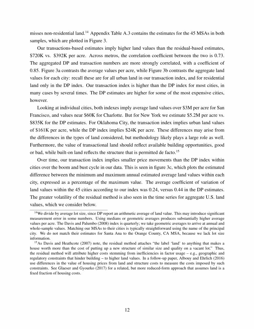
misses non-residential land.14 Appendix Table A.3 contains the estimates for the 45 MSAs in bothsamples, which are plotted in Figure 3.

Our transactions-based estimates imply higher land values than the residual-based estimates,$720K vs. $392K per acre. Across metros, the correlation coefficient between the two is 0.73.The aggregated DP and transaction numbers are more strongly correlated, with a coefficient of0.85. Figure 3a contrasts the average values per acre, while Figure 3b contrasts the aggregate landvalues for each city: recall these are for all urban land in our transaction index, and for residentialland only in the DP index. Our transaction index is higher than the DP index for most cities, inmany cases by several times. The DP estimates are higher for some of the most expensive cities,however.

Looking at individual cities, both indexes imply average land values over $3M per acre for SanFrancisco, and values near $60K for Charlotte. But for New York we estimate $5.2M per acre vs.$835K for the DP estimates. For Oklahoma City, the transaction index implies urban land valuesof $161K per acre, while the DP index implies $24K per acre. These differences may arise fromthe differences in the types of land considered, but methodology likely plays a large role as well.Furthermore, the value of transactional land should reflect available building opportunities, goodor bad, while built-on land reflects the structure that is permitted de facto.15

Over time, our transaction index implies smaller price movements than the DP index withincities over the boom and bust cycle in our data. This is seen in figure 3c, which plots the estimateddifference between the minimum and maximum annual estimated average land values within eachcity, expressed as a percentage of the maximum value. The average coefficient of variation ofland values within the 45 cities according to our index was 0.24, versus 0.44 in the DP estimates.The greater volatility of the residual method is also seen in the time series for aggregate U.S. landvalues, which we consider below.

14We divide by average lot size, since DP report an arithmetic average of land value. This may introduce significantmeasurement error in some numbers. Using medians or geometric averages produces substantially higher averagevalues per acre. The Davis and Palumbo (2008) index is quarterly; we take geometric averages to arrive at annual andwhole-sample values. Matching our MSAs to their cities is typically straightforward using the name of the principalcity. We do not match their estimates for Santa Ana to the Orange County, CA MSA, because we lack lot sizeinformation.

15As Davis and Heathcote (2007) note, the residual method attaches “the label ‘land’ to anything that makes ahouse worth more than the cost of putting up a new structure of similar size and quality on a vacant lot.” Thus,the residual method will attribute higher costs stemming from inefficiencies in factor usage – e.g., geographic andregulatory constraints that hinder building – to higher land values. In a follow-up paper, Albouy and Ehrlich (2016)use differences in the value of housing prices from land and structure costs to measure the costs imposed by suchconstraints. See Glaeser and Gyourko (2017) for a related, but more reduced-form approach that assumes land is afixed fraction of housing costs.

12

Figure 3: Comparison of Transactions-Based Index to Residual-Based Index

(a) Estimated Average Land Values per Acre

Rochester

Pittsburgh

Hartford

Indianapolis

St Louis

Clevleand

AtlantaDetroit

Houston

Dallas

Philadelphia

Minneapolis

Denver

BostonChicago

Portland

WashingtonMiami

San Jose

Los Angeles

San Francisco

New York

1632

6412

525

050

010

0020

0040

0080

00D

avis

and

Pal

umbo

Val

ue p

er E

stim

ated

Acr

e ($

000s

)

125 250 500 1000 2000 4000

Transactions-Based Value per Acre ($000s)

Estimated Values, correlation = 0.83 45-degree line

Best Fit: -12.23 + 1.33 ( 0.13) * AES Est.

(b) Total Land Values

Rochester

Hartford

Indianapolis

Pittsburgh

St Louis

Clevleand

DenverDallas

Portland

Houston

Detroit

Miami

Minneapolis

San Francisco

San JoseBoston

Philadelphia

Atlanta

New York

Chicago

Washington

L.A.

48

1632

6412

525

050

010

00

Dav

is a

nd P

alum

bo L

and

Val

ue p

er L

ottim

es U

rban

Hou

sing

Uni

ts ($

bill

ions

)

16 32 64 125 250 500 1000

Total Transactions-Based Urban Land Value Estimate ($ billions)


Best Fit: -2.84 + 1.37 ( 0.13) * AES Est.

(c) Within-City Time Series Variation

Boston

Rochester

Minneapolis

Denver

San Jose

Chicago

PhiladelphiaNew York

St Louis

WashingtonLos AngelesPittsburgh

San Francisco

Portland

Indianapolis

HoustonHartford

AtlantaClevleand

Miami

Dallas

Detroit

2040

6080

100

Dav

is a

nd P

alum

bo W

ithin

-City

Pric

e V

aria

tion

(%)

20 40 60 80

Transactions-Estimated Within-City Price Variation (%)


Best Fit: 28.24 + 0.63 ( 0.21) * AES Est.

5 Aggregate Urban Land Values over Time

In this section, we sum our urban land values across metros to calculate annual aggregate urbanland values for the United States.16 Table 3 presents these totals.

Over our sample period, average values peaked in 2006 at $624K per acre, an increase of 8%from 2005. Average values then fell to near their 2005 levels in 2007, before declining precipi-

16Our sample includes observations from 324 out of the 331 MSAs and PMSAs in the 1999 OMB definitions. Thecombined imputed land value for the seven metros with no data is $61 billion, less than one-quarter a percent of ouraggregate number.

13

Table 3: Urban Land Values in the United States, 2005-2010

Year

Avg. UrbanLand Value per

Acre($)

Total UrbanLand Value($ billions)

Avg. UrbanLand Value per

Acre (Index,2005 = 100)

Nominal GDP($ billions)

Ratio of TotalUrban Land

Value to GDP

S&P CoreLogicCase-Shiller U.S.

National HPI(Normalized to

2005=100)

Total UrbanLand Value- ResidualMethod

($ billions)

2005 577,336 28,117 100.0 13,094 2.15 100.0 16,7582006 623,950 30,387 108.1 13,856 2.19 106.8 16,9312007 584,682 28,475 101.3 14,478 1.97 104.8 16,0012008 513,413 25,004 88.9 14,719 1.70 95.5 9,5692009 372,819 18,157 64.6 14,419 1.26 86.5 5,7672010 392,683 19,124 68.0 14,964 1.28 84.2 6,234

Land-value data from CoStar COMPS database for years 2005 to 2010. Residual method calculates total real estateholdings at market value of nonfinancial businesses, households, and nonprofit organizations from Financial Ac-counts of the United States (formerly known as the Flow of Funds) and subtracts current-cost net stock of privatestructures from National Income and Product Accounts.

tously. By 2009 the average value was roughly $373K per acre, 65% of its 2005 level. The ratioof aggregate urban land values to gross domestic product declined considerably as well. The ratiowas 2.1–2.2 in 2005 and 2006 before declining to reach a value 1.28 by 2010.

For comparison, we construct a series for aggregate U.S. land values using the residual methodbased on FOF data (now the Financial Accounts of the U.S.). We sum the total value of real estateat market value held by non-financial non-corporate businesses, non-financial corporate businesses,and households and nonprofit organizations to arrive at the total market value of privately held realestate. We then subtract the current-cost net stock of private structures to arrive at a residual-basedvalue for land. In 2006, the estimated value of real estate was $43.3 trillion, while structures werevalued at $26.3T, implying that the total value of land was $16.9T. Our transactions-based estimate,in contrast, is $30.4T, nearly 80% higher.

In addition to the methodological differences, the totals may differ because they cover differentland. Our estimates are based on total metro urban areas, including public lands for roads, parks,and civic buildings. Assuming that the public owns urban land worth 40% of the total value, only$18.2T of land would be owned privately, which is much closer to the FOF numbers. On the otherhand, the FOF numbers include land outside of metro-urban areas, which we exclude.

Land values calculated from the FOF fell even more dramatically than our series, down to only$5.8T in 2009, as opposed $14.4T. The peak-to-trough decline in the transactions-based index was40%, substantially less than the 66% decline in the FOF.

Last, we consider how land values compare with housing prices. The final column of table 3 re-ports the S&P CoreLogic Case-Shiller U.S. National House Price Index, normalized to have value

14

100 in 2005. Overall, land values appear to have led house prices slightly, and were substantiallymore volatile than house prices over the sample period. This result is consistent with the Bosticet al. (2007) land leverage hypothesis that housing should have less volatile values than land.

6 Conclusion

Our analysis combines insights from the monocentric city model with empirical Bayesian methodsto produce novel and plausible estimates of land values, even in metros with relatively thin data.These methods might easily be applied to estimate other city-wide measures, such as wages orproperty prices. Relative to residual approaches, our method suggests that urban land values maybe higher, less volatile, and less likely to be negative. Furthermore, the model sheds light onthe enormous differences in land values both across and within cities, with high central valuesproviding indirect support for monocentric cities, albeit with heterogeneous value gradients.

We hope that the measures we provide may form the basis of reliable estimates of aggregateland wealth. With additional data, future modeling could be enriched to incorporate greater spatialstructure and modifications for observed land uses. The cross-sectional index we provide shouldalso prove useful to researchers examining differences in amenities and costs across metro areas.

References

David Albouy. What are cities worth? land rents, local productivity, and the total value of ameni-ties. Review of Economics and Statistics, 98(3):477–487, 2016.

David Albouy and Gabriel Ehrlich. Housing productivity and the social cost of land use restric-tions. NBER Working Paper, 18110, 2016.

William Alonso. Location and land use. Toward a general theory of land rent. Harvard UniversityPress, 1964.

Jason Barr, Fred Smith, and Sayali Kulkarni. What’s manhattan worth? a land values index from1950 to 2014. Rutgers University, 2016.

Raphael W Bostic, Stanley D Longhofer, and Christian L Redfearn. Land leverage: decomposinghome price dynamics. Real Estate Economics, 35(2):183–208, 2007.

Jan K. Brueckner. Property value maximization and public-sector efficiency. Journal of Urban

Economics, 14:1–15, 1983.Bureau of Economic Analysis. Relation of BEA’s Current-Cost Net Stock of Private Structures to

the corresponding items in the Federal Reserve Board’s Financial Accounts of the United States.Technical report, 2013. URL https://www.bea.gov/national/pdf/st13.pdf.

15

https://www.bea.gov/national/pdf/st13.pdf

Karl Case. The value of land in the united states: 1975-2005. In GK Ingram and Y.-H. Hong,editors, Land Policies and Their Outcomes. Lincoln Institute of Land Policy, 2007.

Peter F Colwell and Henry J Munneke. The structure of urban land prices. Journal of Urban

Economics, 41(3):321–336, 1997.Peter F Colwell and Clemon F Sirmans. A comment on zoning, returns to scale, and the value of

undeveloped land. The Review of Economics and Statistics, pages 783–786, 1993.Pierre-Philippe Combes, Gilles Duranton, and Duranton Gobillon. The costs of agglomeration:

House and land prices in french cities. mimeo, 2016.Morris A Davis and Jonathan Heathcote. The price and quantity of residential land in the united

states. Journal of Monetary Economics, 54(8):2595–2620, 2007.Morris A Davis and Michael G Palumbo. The price of residential land in large us cities. Journal

of Urban Economics, 63(1):352–384, 2008.Jeff Fisher, David Geltner, and Henry Pollakowski. A quarterly transactions-based index of insti-

tutional real estate investment performance and movements in supply and demand. Journal of

Real Estate Finance and Economics, 34:5–33, 2007.Henry George. Progress and poverty: An inquiry into the cause of industrial depressions, and of

increase of want with increase of wealth, the remedy. W. Reeves, 1884.Edward L Glaeser and Joseph Gyourko. Urban decline and durable housing. Journal of political

economy, 113(2):345–375, 2005.Edward L Glaeser and Joseph Gyourko. The economic implications of housing supply. Zell/Lurie

Wroking Paper, 802, 2017.D. A. Harville. Maximum likelihood approaches to variance component estimation and to related

problems. Journal of the American Statistical Association, 72(358):320–338, 1977.Andrew Haughwout, James Orr, and David Bedoll. The price of land in the new york metropolitan

area. Federal Reserve Bank of New York Current Issues in Economics and Finance, 2008.Nils Kok, Paavo Monkkonen, and John M Quigley. Land use regulations and the value of land and

housing: An intra-metropolitan analysis. Journal of Urban Economics, 81:136–148, 2014.Nan M. Laird and Thomas A. Louis. Empirical bayes ranking methods. Journal of Education

Statistics, 14(1):29–46, 1989.William Larson et al. New estimates of value of land of the united states. Technical report, Bureau

of Economic Analysis, 2015.Edwin S. Mills. An aggregative model of resource allocation in a metropolitan area. American

Economic Review, 57:197–210, 1967.Henry Munneke and Slade Barrett. An empirical study of sample-selection bias in indices of

commercial real estate. Journal of Real Estate Finance and Economics, 21:45–64, 2000.

16

Henry Munneke and Slade Barrett. A metropolitan transaction-based commercial price index: Atime-varying parameter approach. Real Estate Economics, 29:55–84, 2001.

Richard F Muth. Cities and Housing: the Spatial Pattern of Urban Residential Land Use. Univer-sity of Chicago Press, 1969.

Joseph B Nichols, Stephen D Oliner, and Michael R Mulhall. Swings in commercial and residentialland prices in the united states. Journal of Urban Economics, 73(1):57–76, 2013.

Adam Ozimek, Daniel Miles, et al. Stata utilities for geocoding and generating travel time andtravel distance information. Stata Journal, 11(1):106, 2011.

David Ricardo. On the principles of political economy, and taxation. John Murray, 1821.Jennifer Roback. Wages, rents, and the quality of life. Journal of Political Economy, 90:1257–

1258, 1982.S.L. Zeger and M.R. Karim. Generalized linear models with random effects: A gibbs sampling

approach. Journal of the American Statistical Association, 86, 1991.

17

A Appendix for Online Publication

A.1 Additional Data NotesWhen a CMSA contains multiple PMSAs, we treat each PMSA as its own MSA for purposes ofestimation and reporting. For instance, we treat the Washington, DC-MD-VA-WV and Baltimore,MD PMSAs as separate MSAs, although they are both parts of the Washington-Baltimore DC-MD-VA-WV CMSA. For New York City we use the Empire State Building as the city centerrather than City Hall, following Haughwout et al. (2008). We treat each named city in an MSAwith a hyphenated city name as having its own city center. For instance, we treat Minneapolis-St.Paul, MN-WI as containing two distinct cities, Minneapolis, MN, and St. Paul, MN. However, wetreat such cities as belonging to one MSA for purposes of estimation and reporting. We excludeMSAs located in Puerto Rico from the analysis.

In the CoStar data, we consider 12 of the most common proposed uses, which are neithermutually exclusive nor collectively exhaustive. We consider an observation to feature a structurewhen the transaction record includes the fields for “ Bldg Type”, “ Year Built”, “ Age”, or thephrase “ Business Value Included” in the field “ Sale Conditions.” We geocoded the lot sales usingthe Stata “geocode” module of Ozimek et al. (2011). In addition to the exclusions discussed inthe main text, we also exclude outlier observations with a listed price of less than $100 per acreor a lot size over 5,000 acres, or further than 60 miles away from the city center. We also excludelocations we could not geocode successfully.

Median lot size is 3.5 acres versus a mean of 26 acres. Land sales occur more frequently inthe beginning of our sample period, with 21.7% of our sample from 2005 and 11.4% from 2010.Residential uses are common but by no means predominant in the sample: 17.6% of properties havea proposed use of single-family, multifamily, or apartments. 23.4% is being held for developmentor investment, and 16% of the sample had no listed proposed use.

B Computation

B.1 Estimation of αjt and δjFor notational convenience we rewrite the model in (1) as

ln rijt = Z ′ijtγj +Xijtβ + eijt, eijt ∼ N(0, σ2e), (A.1)

where Z ′ijt =[1, Dij, D

2ij, D

3ij, D

4ij, 1

2006ijt , 1

2007ijt , 1

2008ijt , 1

2009ijt , 1

2010ijt

], with Dij = D(zij, z

cj), and

where 1sijt is an indicator variable that takes value 1 if s = t and 0 otherwise. The parameter vectorγj collects city and time specific parameters with a multivariate normal prior distribution

γj = [αj, δj1, δj2, δj3, δj4, αj,2006, αj,2007, αj,2008, αj,2009, αj,2010]′ ∼ N(mγ,j, Vγ,0) (A.2)

where

mγ,j =

a0 + a1Ajb0 + b1Aj

τ

and Vγ,0 =

Σαα Σαδ 0(1×5)Σδα Σδδ 0(4×5)

0(5×1) 0(5×4) Σττ

(A.3)

i

with τ = [τ2006, τ2007, τ2008, τ2009, τ2010]′ and Σττ = diag([σ2

2005, σ22006, σ

22007, σ

22008, σ

22009, σ

22010]

′).Conditional on fixed and variance parameters (θ = [β, a0, a1,b0,b1, τ, σ

2e ,Σαα,Σδα,Σττ ]) and

observed data for city j, the posterior distribution of γj follows the multivariate normal distribution

γj|θ,Data ∼ N(mγ,j(θ), Vγ,j(θ)

)(A.4)

with a posterior mean as the weighted average between the prior mean (mγ,0) and the fixed effectestimate γj = (Z ′jZj)

−1 [Z ′j (ln rj −Xjβ)]:

mγ,j(θ) = Wj(θ)mγ,j + [I −Wj(θ)] γj(θ) where Wj(θ) =[V −10 + σ−2e (Z ′jZj)

]−1V −10 . (A.5)

Here we write Zj , ln rj , and Xj as matrices that stack elements only relevant for the city j. Theweight depends on the number of observations in the city j (nj), the relative size of the priorvariance (Vj) and the idiosyncratic shock variance (σ2). The posterior variance is

Vγ,j(θ) =[V −10 + σ−2e (Z ′jZj)

]−1. (A.6)

It is well known that the posterior mean mγ,j(θ) is the best linear unbiased predictor for γj givenθ and the observed data. In our application, we do not know θ. Instead of taking a full Bayesianapproach and putting a prior on θ, we take the empirical Bayesian approach in which θ is calibratedby maximizing the following marginal likelihood (Laird and Louis, 1989):

θ ∈ argminθ L(data|θ) =

∫p(ln rijt|Z,X, θ, γ)dγ (A.7)

where the γ is integrated out from the conditional posterior distribution an improper prior, p(γ) ∝1, viz. Harville (1977). Then, we treat θ as a known and fixed quantity and use the followingposterior distribution for the computation of land values and the prediction,

γj|Data ∼ N(mγ,j(θ), Vγ,j(θ)

). (A.8)

One of the potential shortcomings of this approach is that it neglects uncertainty coming from theestimation of θ, and the resulting posterior distribution for γj underestimates uncertainty. For-tunately, we have a relatively large amount of data about θ (about 67,000 observations in total).Second, the practicality of our shrinkage estimator is evaluated by the out-of-sample forecastingevaluation. However, we note that a full Bayesian approach is possible (Zeger and Karim, 1991)at the cost of longer computation time. We choose to take the empirical Bayes approach becauseof the out-of-sample evaluation of our shrinkage procedure.

B.2 Point predictionOnce we obtain the posterior distribution of γj , we can generate land value predictions. For thecross-validation exercise, we generate and evaluate point predictions for the log-price of the landparcels in the city j at time twith characteristicX∗ijt and Z∗ijt as the mean of the posterior predictivedistribution. When the land parcel the value of which we predict is in a city j that has observed

ii

data, this point prediction is

ln rijt =

∫ln rijtp(ln rijt|data,X∗ijt, Z∗ijt)d ln rijt

=

∫ ∫ln rijtp(ln rijt|data,X∗ijt, Z∗ijt, γj)p(γj|data)dγjd ln rijt

= Z∗′

ijtmγ,j(θ) +X∗′

ijtβ.

(A.9)

We can also generate predictions for the land parcels that are in a “missing” city where we do nothave observed transaction prices. In this case, our prediction is just

ln rijt = Z∗′

ijtmγ,j(θ) +X∗′

ijtβ, (A.10)

where our prediction is based on the prior with estimated hyperparameters, θ.

B.3 Computation of Land valuesFor each census tract l in city j in year t, we calculate the predicted land value rljt at the tractcentroid and assign that average value to the entire tract.

Rjt =L∑l=1

rljtAl (A.11)

where Al is the tract area we use the mean of the predictive distribution for rljt as the predictedland value. That is,

rljt =

∫exp(rljt)p(rljt|data,X∗∗ljt, Z∗∗ljt)drljt

=

∫ ∫exp(rljt)p(rljt|data,X∗∗ljt, Z∗∗ljt, γj)p(γj|data)drljtdγj

= exp(Z∗∗

′

ljtmγ,j(θ) +X∗∗′

ljt β + 1/2σ2e + 1/2Z∗∗

′

ljt Vγ,j(θ)Z∗∗′ljt

) (A.12)

where the last two terms are due to the log-normal correction. We can also estimate values forcities with no observed land sales using only the prior.

In our application some of land characteristics such as lot sizes and planned uses (a subvectorof X∗∗ljt) are unknown at the tract centroid, and therefore they need to be predicted as well. To deal

iii

with this issue we decompose the predicted land value in the following manner:

rljt =

∫exp(rljt)p(rljt|data,X∗∗ljt, Z∗∗ljt)drljt

=

∫ ∫exp(rljt)p(rljt|data,X∗∗ljt, Z∗∗ljt, γj)p(γj, X∗∗ljt|data, Z∗∗ljt)drljtdγjdX∗∗ljt

=

∫ ∫exp(rljt)p(rljt|data,X∗∗ljt, Z∗∗ljt, γj)p(γj|data)p(X∗∗ljt|data, Z∗∗ljt)drljtdγjdX∗∗ljt

= exp(Z∗∗

′

ljtmγ,j(θ) + 1/2σ2e + 1/2Z∗∗

′

ljt Vγ,j(θ)Z∗∗′ljt

)∫exp

(X∗∗

′

ljt β)p(X∗∗ljt|data, Z∗∗ljt)dX∗∗ljt

(A.13)

where the uncertainty about the unobserved land characteristic at the tract centroid is capturedby the predictive distribution function of X∗∗ljt in the last integral. We construct a model for eachunobserved element in X∗∗ljt using observed characteristics of the tract l in city j. More specifically,s-th element in X∗∗s,ljt is modeled as

X∗∗s,ljt = αxs,j + δxs,jDlj + γsClj + es,ljt, es,ljt ∼ i.i.d.N(0, σ2s) (A.14)

where Dlj is the distance metric based on the distance between the tract centroid and the citycenter, and Clj is log distance to coast from the tract centroid.

This technique is based on a similar but simpler version of the hierarchical model used for landprices. The intercept and coefficient on the distance to the city center are allowed to vary acrossMSAs, but using only an affine function, as opposed to a quartic polynomial. The coefficient onthe distance to the coast is fixed.

Because these coefficients are not known, we estimate them using the observed transactiondata with the similar prior specification and assumption employed for the estimation of model forthe land price. More specifically, the prior distribution for city-specific parameters αxs,j and δxs,jfollow multivariate normal distribution, where its mean vector is an affine function of each city’surban area and its variance-covariance matrix is allowed to have non-zero off-diagonal elements.We impose similar exogeneity assumptions for αxs,j , δ

xs,j , and es,ljt. Lastly, we assume that each

element in X∗∗ljt are correlated only through observed tract characteristics Dlj and Clj (equationA.14). Because estimation and prediction for the land price and land characteristics are performedconditional on distance variables, we do not assume any specific distributional form for observeddistance variables Dij and Cij . However, we assume that the marginal density of Dij puts non-zero positive value on the entire MSA area. This last assumption implies that if we do not havea transaction observation at a specific census tract, this missingness is completely random and wewould eventually collect observations from this tract as the sample size goes to infinity.

B.4 Cross-validationThe cross-validation technique helps to evaluate the effectiveness of the econometric specificationand shrinkage model. We design a pseudo out-of-sample prediction exercise that quantifies thepotential gains or losses from different models. For this exercise we take cities that have at least 50observations per year for at least two years This leads to 58 cities with 55,155 total observations.

iv

Then, for each city j,

1. Randomly choose nhold observations out of njt observations for each time t = 2005, 2006, ..., 2010in city j. We keep those 6 ∗ nhold observations as well as the remaining sample of data fromother cities.

2. Estimate each of models using the method described in subsection B.1

3. Generate predictions for sample held out in step 1 for city j based on the method in subsec-tion B.2

4. Compute and store the prediction error for this hold-out samples. {ej,r,1, ej,r,2, ..., ej,r,(njt−nhold)}(forecast errors are defined as predicted minus actual).

5. Repeat Step 1 – Step 4 for r = 1, 2, ..., R.

6. Repeat Step 1 – Step 5 for each city j = 1, , J .

7. Compute aggregated out-of-sample prediction evaluation statistics. For example, the MSEfor the city j is computed as

MSE(j) =1

R× (nj,t − nhold)

R∑r=1

(njt−nhold)∑i=1

e2r,j,i (A.15)

where we set R = 30. We perform for nhold = 3 (small sample size) and nhold = 30 (moderatesample size) for each city. About 35% of MSAs in our sample have observations less than equal to18 observations (which is approximately 3 per year in our data set) and about 81% of MSAs in oursample have observations less than equal to 180 (which is approximately 30 per year in our dataset). We report average MSE(j) over j = 1, 2, ...58.

Unshrunken Estimator. The unshrunken estimates are based on the fixed effect estimation. Theestimator is defined as γj = (Z ′jZj)

−1(Z ′j(ln rj −Xjβ) and used in Equation A.5.

v

Table A.1: Estimated Coefficients on Covariates in Preferred Specification

CovariateEstimatedCoefficient

StandardError t-statistic p-value

Log Lot Size -0.543 0.0037 -146.134 0.000(Log Lot Size Squared)/100 -3.053 0.1592 -19.176 0.000(Log Lot Size Cubed)/1000 3.601 0.2498 14.415 0.000Log Distance to Coast -0.052 0.0043 -12.196 0.000

Planned Use:None Listed -0.182 0.0112 -16.193 0.000Commercial -0.380 0.0599 -6.354 0.000Industrial -0.346 0.0141 -24.578 0.000Retail 0.255 0.0134 18.963 0.000Single Family 0.003 0.0133 0.202 0.840Multifamily -0.139 0.0198 -7.055 0.000Office 0.046 0.0148 3.129 0.002Apartment 0.288 0.0196 14.713 0.000Hold for Development -0.073 0.0118 -6.171 0.000Hold for Investment -0.283 0.0195 -14.523 0.000Mixed Use 0.250 0.0265 9.438 0.000Medical 0.171 0.0355 4.810 0.000Parking 0.076 0.0373 2.044 0.041

This table reports the coefficients on the covariates from the preferred specificationin table 1 from the main body of the text, which applies shrinkage to a model with aquartic polynomial in log distance to the city center plus one mile.

vi

Table A.2: Metropolitan Land Value Indices Ranked by Average Urban Land Value per Acre, 2005-2010




No. ofLandSales

NaiveModel Central

UrbanAvg.


Total Est.Urban


1 New York, NY 749 1,603 26,139 123,335 5,264 22.3 2,524.42 Jersey City, NJ 47 43 7,667 9,554 3,305 8.8 98.83 Honolulu, HI 198 56 4,357 16,256 3,290 7.0 416.34 San Francisco, CA 300 152 8,722 25,446 3,239 9.3 622.85 Los Angeles-Long Beach, CA 1,359 1,760 3,709 16,801 2,675 5.5 2,326.86 Orange County, CA 494 233 3,163 3,208 2,595 1.3 820.57 San Jose, CA 305 217 2,580 3,552 2,347 1.6 458.38 Miami, FL 372 1,233 3,052 4,478 1,794 3.2 427.59 Stamford-Norwalk, CT 179 19 2,753 2,740 1,505 3.2 172.410 Bergen-Passaic, NJ 316 79 1,957 4,145 1,423 3.7 287.711 Oakland, CA 495 132 2,648 5,447 1,412 3.3 447.112 Fort Lauderdale, FL 372 741 2,417 3,572 1,336 3.1 318.013 Seattle-Bellevue-Everett, WA 782 1,626 2,741 9,930 1,317 10.1 658.614 West Palm Beach-Boca Raton, FL 398 321 2,188 5,990 1,305 5.3 332.815 Santa Barbara-Santa Maria-Lompoc, CA 159 29 2,345 2,511 1,237 2.8 126.216 Washington, DC-MD-VA-WV 1,458 1,840 3,548 36,913 1,214 32.6 1,133.017 San Luis Obispo-Atascadero-Paso Robles, CA 91 43 1,416 1,563 1,174 1.6 68.418 Santa Cruz-Watsonville, CA 72 12 2,007 2,279 1,163 4.3 53.319 San Diego, CA 803 957 2,488 10,081 1,073 8.7 551.020 Nassau-Suffolk, NY 850 396 1,540 800 931 0.8 506.421 Newark, NJ 567 142 2,059 5,436 872 5.0 316.722 Las Vegas, NV-AZ 317 2,553 1,193 1,841 849 2.4 172.4

vii





No. ofLandSales

NaiveModel Central

UrbanAvg.


Total Est.Urban


23 Naples, FL 145 78 791 1,081 738 1.5 68.524 Ventura, CA 202 131 1,048 1,537 692 2.4 89.725 Portland-Vancouver, OR-WA 527 1,191 777 6,063 679 11.5 228.926 Chicago, IL 2,035 3,511 1,455 37,632 663 35.1 863.327 Boston, MA-NH 1,295 122 1,243 8,457 600 9.8 497.528 Santa Rosa, CA 144 153 1,034 956 590 2.2 54.329 Anchorage, AK 94 21 851 490 572 1.3 34.430 Provo-Orem, UT 105 47 499 963 568 2.1 38.231 Salt Lake City-Ogden, UT 411 145 482 1,228 557 2.2 146.332 Denver, CO 536 2,015 828 7,586 539 18.6 185.133 Vallejo-Fairfield-Napa, CA 129 146 786 984 539 2.4 44.334 Tacoma, WA 308 539 570 2,427 530 5.6 104.435 Sarasota-Bradenton, FL 260 601 893 975 514 2.1 85.636 Providence-Fall River-Warwick, RI-MA 439 62 1,194 2,139 508 7.4 142.737 Panama City, FL 101 41 815 385 502 0.7 32.638 Baltimore, MD 858 802 969 2,281 501 4.1 275.239 Bridgeport, CT 200 26 837 1,581 500 3.5 63.940 Salinas, CA 101 12 814 1,023 490 2.6 31.641 Minneapolis-St. Paul, MN-WI 1,026 846 613 3,323 486 6.4 318.842 Middlesex-Somerset-Hunterdon, NJ 424 101 828 1,302 482 3.1 130.943 Fort Walton Beach, FL 86 14 300 930 478 2.4 26.344 Reno, NV 125 57 530 1,150 472 4.1 37.9

viii





No. ofLandSales

NaiveModel Central

UrbanAvg.


Total Est.Urban


45 Yolo, CA 34 50 624 640 468 1.5 10.146 Barnstable-Yarmouth, MA 188 3 387 1,090 466 3.0 56.047 Fort Myers-Cape Coral, FL 240 294 593 345 465 0.7 71.448 Gary, IN 285 111 468 2,428 463 8.4 84.549 Fort Pierce-Port St. Lucie, FL 180 71 475 657 463 1.9 53.450 Tampa-St. Petersburg-Clearwater, FL 957 1,220 1,144 3,037 454 7.5 278.151 Lowell, MA-NH 161 12 544 1,056 453 3.1 46.652 Phoenix-Mesa, AZ 897 5,946 370 3,529 452 8.4 259.453 Charleston-North Charleston, SC 238 214 498 2,569 446 11.0 67.854 Sacramento, CA 412 448 602 2,121 442 4.7 116.755 Orlando, FL 666 1,612 739 3,191 431 6.9 183.956 Monmouth-Ocean, NJ 524 124 642 2,044 425 5.4 142.557 Albuquerque, NM 281 114 413 635 418 1.5 75.058 Charlottesville, VA 47 4 728 589 415 2.2 12.459 Punta Gorda, FL 98 63 648 963 406 2.6 25.460 Atlantic-Cape May, NJ 174 37 538 1,298 406 4.1 45.261 Wilmington, NC 139 50 420 830 402 2.2 35.862 Stockton-Lodi, CA 130 163 531 423 399 1.0 33.163 Colorado Springs, CO 199 892 409 830 396 2.4 50.564 New Haven-Meriden, CT 270 43 658 1,745 396 6.1 68.465 Modesto, CA 120 142 407 707 388 2.3 29.966 Boulder-Longmont, CO 91 183 758 462 387 1.9 22.5

ix





No. ofLandSales

NaiveModel Central

UrbanAvg.


Total Est.Urban


67 Danbury, CT 160 23 426 1,003 368 4.3 37.868 Bremerton, WA 130 18 465 856 367 2.7 30.569 Madison, WI 130 239 468 2,815 365 13.9 30.470 Philadelphia, PA-NJ 1,725 859 939 13,254 362 29.4 400.171 Myrtle Beach, SC 97 84 507 1,000 360 4.1 22.472 Burlington, VT 68 5 790 773 358 3.7 15.773 Trenton, NJ 127 35 432 800 354 2.7 28.974 Boise City, ID 158 106 294 601 349 1.9 35.375 Lawrence, MA-NH 236 29 410 1,178 344 5.1 51.976 Reading, PA 124 36 324 529 342 2.0 27.177 Visalia-Tulare-Porterville, CA 104 32 614 557 340 3.7 22.778 La Crosse, WI-MN 44 21 295 488 339 2.5 9.679 Norfolk-Virginia Beach-Newport News, VA-NC 554 392 377 1,375 337 5.0 119.480 Monroe, LA 78 7 360 605 336 3.3 16.881 Tallahassee, FL 125 52 474 1,001 335 5.6 26.982 Iowa City, IA 36 9 423 428 334 2.5 7.683 Salem, OR 109 54 356 868 334 3.4 23.284 Olympia, WA 105 250 455 543 333 2.5 22.585 New Orleans, LA 364 66 672 1,690 332 5.9 77.586 Bellingham, WA 57 19 286 514 331 2.4 12.287 Springfield, MA 252 28 523 1,336 328 5.4 52.988 New Bedford, MA 72 14 503 597 326 3.1 15.1

x





No. ofLandSales

NaiveModel Central

UrbanAvg.


Total Est.Urban


89 Lexington, KY 138 29 345 564 320 1.9 28.290 Spokane, WA 160 55 603 1,389 318 6.4 32.691 Jacksonville, FL 497 793 559 776 316 2.3 100.692 Riverside-San Bernardino, CA 971 2,452 433 637 315 1.5 195.593 El Paso, TX 206 94 321 399 313 1.2 41.394 Daytona Beach, FL 225 93 539 368 312 1.2 45.095 Portsmouth-Rochester, NH-ME 133 13 291 581 310 2.6 26.496 Portland, ME 120 25 1,399 869 309 3.6 23.897 Grand Junction, CO 60 21 343 565 307 2.8 11.898 Nashville, TN 580 455 499 1,499 306 4.7 113.699 Dallas, TX 1,057 811 454 2,774 305 10.1 206.4100 Richland-Kennewick-Pasco, WA 95 27 273 357 300 1.7 18.3101 Wilmington-Newark, DE-MD 215 107 445 607 298 3.1 40.9102 Tucson, AZ 325 1,749 320 914 296 3.3 61.5103 Columbus, GA-AL 114 11 250 620 294 3.3 21.5104 Medford-Ashland, OR 66 12 379 465 293 2.5 12.4105 Austin-San Marcos, TX 423 384 434 3,054 293 12.8 79.3106 Melbourne-Titusville-Palm Bay, FL 255 420 688 353 293 1.3 47.8107 Gainesville, FL 79 34 384 527 292 3.8 14.8108 Merced, CA 61 64 319 455 288 2.1 11.2109 Chattanooga, TN-GA 303 51 387 1,367 283 5.8 54.8110 Sioux Falls, SD 49 17 306 372 283 2.5 8.9

xi





No. ofLandSales

NaiveModel Central

UrbanAvg.


Total Est.Urban


111 Santa Fe, NM 78 7 335 539 282 2.2 14.1112 Green Bay, WI 83 49 289 340 282 2.3 15.1113 Greenville, NC 47 9 259 460 279 3.5 8.4114 Yuba City, CA 42 13 890 625 278 6.6 7.4115 Raleigh-Durham-Chapel Hill, NC 532 782 497 627 276 2.5 94.2116 Waterbury, CT 125 9 243 437 275 2.2 21.9117 Bakersfield, CA 161 64 250 625 272 2.0 28.0118 Houston, TX 1,341 1,143 423 2,813 272 9.4 233.1119 Joplin, MO 72 8 255 450 271 2.7 12.5120 Detroit, MI 1,426 679 456 2,321 270 6.6 246.6121 Las Cruces, NM 88 18 240 430 270 2.3 15.2122 Fort Collins-Loveland, CO 91 344 417 348 270 1.4 15.7123 Fresno, CA 215 137 247 453 266 1.8 36.7124 Cincinnati, OH-KY-IN 645 637 441 1,656 266 6.7 109.8125 Abilene, TX 49 3 356 337 266 2.5 8.4126 Fayetteville-Springdale-Rogers, AR 135 43 356 293 263 1.7 22.7127 Eugene-Springfield, OR 92 36 413 598 262 4.1 15.4128 Worcester, MA-CT 248 56 454 1,918 261 11.2 41.3129 Lawrence, KS 26 6 266 293 252 2.1 4.3130 Atlanta, GA 2,105 5,229 402 1,750 251 5.5 338.6131 Fargo-Moorhead, ND-MN 46 13 470 274 251 1.7 7.4132 Omaha, NE-IA 237 118 633 1,147 251 4.7 38.0

xii





No. ofLandSales

NaiveModel Central

UrbanAvg.


Total Est.Urban


133 Cleveland-Lorain-Elyria, OH 745 416 545 713 251 2.4 119.7134 Greeley, CO 48 320 302 359 246 2.1 7.5135 Huntsville, AL 179 29 190 519 244 2.3 28.0136 Lincoln, NE 78 24 258 430 243 3.5 12.1137 Billings, MT 53 25 297 319 243 2.5 8.2138 Harrisburg-Lebanon-Carlisle, PA 243 89 334 1,084 242 7.7 37.7139 Manchester, NH 97 23 230 559 240 3.9 14.9140 Fort Worth-Arlington, TX 693 506 313 566 239 2.3 105.8141 Louisville, KY-IN 413 126 279 650 233 2.7 61.6142 Baton Rouge, LA 292 99 308 907 228 3.6 42.7143 Janesville-Beloit, WI 56 15 277 301 226 3.1 8.1144 McAllen-Edinburg-Mission, TX 318 61 400 398 226 2.6 45.9145 Asheville, NC 126 41 318 499 226 3.0 18.1146 Columbus, OH 512 671 614 1,238 222 5.5 72.8147 Tulsa, OK 332 245 323 744 222 3.0 47.1148 Bloomington-Normal, IL 39 10 193 264 220 2.8 5.5149 Milwaukee-Waukesha, WI 542 399 313 821 219 3.8 76.0150 Dubuque, IA 31 4 210 266 219 2.3 4.4151 Anniston, AL 77 4 214 397 218 2.8 10.8152 Waterloo-Cedar Falls, IA 53 12 229 298 215 2.5 7.3153 Rocky Mount, NC 52 12 292 299 215 1.9 7.1154 Roanoke, VA 111 23 208 442 214 2.9 15.2

xiii





No. ofLandSales

NaiveModel Central

UrbanAvg.


Total Est.Urban


155 Nashua, NH 96 3 147 426 212 3.1 13.0156 Columbia, MO 54 3 206 333 212 2.8 7.3157 Hagerstown, MD 49 28 348 518 212 9.5 6.6158 Richmond-Petersburg, VA 441 399 293 1,509 212 8.4 59.7159 Brockton, MA 148 22 362 528 212 3.3 20.1160 Galveston-Texas City, TX 116 39 267 445 211 2.1 15.7161 Allentown-Bethlehem-Easton, PA 264 85 281 348 211 2.3 35.6162 Missoula, MT 36 4 374 311 210 2.6 4.9163 Lake Charles, LA 99 14 206 441 209 3.4 13.3164 Decatur, IL 50 2 239 331 209 3.4 6.7165 Champaign-Urbana, IL 58 22 262 338 207 4.1 7.6166 Savannah, GA 128 64 337 370 204 1.9 16.7167 Kansas City, MO-KS 698 477 342 565 202 2.4 90.4168 St. Louis, MO-IL 979 364 337 700 200 3.1 125.5169 Little Rock-North Little Rock, AR 244 110 305 528 200 3.0 31.2170 Decatur, AL 39 5 533 402 196 4.3 5.0171 Birmingham, AL 421 148 238 298 196 1.4 52.9172 Rochester, MN 43 7 189 253 196 3.1 5.4173 Steubenville-Weirton, OH-WV 54 1 122 268 195 2.3 6.7174 Indianapolis, IN 649 193 274 858 195 3.8 80.9175 Hamilton-Middletown, OH 124 151 372 96 195 0.3 15.4176 Auburn-Opelika, AL 62 5 233 267 195 1.8 7.8

xiv





No. ofLandSales

NaiveModel Central

UrbanAvg.


Total Est.Urban


177 York, PA 180 47 176 460 194 2.5 22.4178 Laredo, TX 47 2 255 300 194 2.5 5.9179 Dayton-Springfield, OH 382 116 317 777 194 5.1 47.4180 Flagstaff, AZ-UT 35 7 294 230 194 1.9 4.4181 Springfield, MO 124 43 261 487 194 4.0 15.3182 San Antonio, TX 468 348 224 710 192 3.7 57.6183 Pensacola, FL 246 102 317 669 192 3.6 30.3184 Columbia, SC 270 139 237 871 190 6.5 32.8185 Redding, CA 78 8 150 289 189 2.0 9.4186 Hartford, CT 616 101 672 1,139 188 6.3 74.1187 Lancaster, PA 229 57 176 597 188 4.7 27.5188 Fayetteville, NC 156 25 476 253 184 1.7 18.4189 Greensboro–Winston Salem–High Point, NC 602 438 297 274 183 1.6 70.4190 Knoxville, TN 400 193 265 496 181 2.5 46.3191 Houma, LA 93 4 102 474 180 3.1 10.7192 Jacksonville, NC 94 6 134 368 180 2.4 10.8193 St. Cloud, MN 45 17 331 252 179 2.3 5.1194 Newburgh, NY-PA 169 54 206 504 178 3.1 19.2195 Yakima, WA 74 15 182 289 178 1.9 8.4196 Tuscaloosa, AL 76 16 252 349 177 3.3 8.6197 Bangor, ME 38 5 339 347 176 3.4 4.3198 Biloxi-Gulfport-Pascagoula, MS 172 30 163 424 173 3.6 19.0

xv





No. ofLandSales

NaiveModel Central

UrbanAvg.


Total Est.Urban


199 Kenosha, WI 64 58 604 161 173 1.2 7.1200 Lakeland-Winter Haven, FL 247 561 324 283 172 2.0 27.2201 Duluth-Superior, MN-WI 81 22 344 133 172 1.7 8.9202 Ann Arbor, MI 231 136 293 1,227 172 12.3 25.4203 New London-Norwich, CT-RI 166 31 299 296 171 1.7 18.2204 Clarksville-Hopkinsville, TN-KY 96 60 213 274 171 2.4 10.5205 Dutchess County, NY 158 33 588 804 170 6.6 17.2206 Pine Bluff, AR 35 2 232 215 167 2.2 3.8207 Springfield, IL 94 11 430 335 166 4.3 10.0208 Cumberland, MD-WV 41 6 145 283 166 2.5 4.3209 Grand Rapids-Muskegon-Holland, MI 435 121 243 537 166 4.9 46.2210 Vineland-Millville-Bridgeton, NJ 72 11 410 261 166 3.7 7.6211 Lafayette, IN 61 13 190 192 164 1.5 6.4212 Jackson, MS 192 43 191 753 164 6.1 20.2213 Eau Claire, WI 63 30 123 225 164 1.7 6.6214 Buffalo-Niagara Falls, NY 395 104 616 1,157 162 8.6 41.1215 Memphis, TN-AR-MS 423 173 328 572 162 4.1 43.9216 Waco, TX 73 14 185 227 161 2.2 7.6217 Oklahoma City, OK 391 395 285 280 161 1.5 40.3218 Bismarck, ND 34 22 155 153 161 1.5 3.5219 Johnson City-Kingsport-Bristol, TN-VA 273 28 169 284 160 2.2 28.0220 Brownsville-Harlingen-San Benito, TX 125 52 263 159 159 0.8 12.8

xvi





No. ofLandSales

NaiveModel Central

UrbanAvg.


Total Est.Urban


221 Canton-Massillon, OH 189 40 220 264 159 2.3 19.2222 Des Moines, IA 158 99 238 776 158 5.5 16.1223 Augusta-Aiken, GA-SC 243 66 228 250 158 1.6 24.6224 South Bend, IN 126 12 118 335 157 3.3 12.7225 Dover, DE 54 7 151 253 157 2.5 5.4226 Yuma, AZ 54 12 215 355 156 3.2 5.4227 Pittsburgh, PA 1,003 240 433 1,772 156 10.6 100.0228 Amarillo, TX 85 27 173 215 155 2.2 8.4229 Terre Haute, IN 54 4 200 237 151 2.1 5.2230 Akron, OH 337 169 349 446 150 2.9 32.4231 Texarkana, TX-Texarkana, AR 70 5 118 225 150 2.6 6.7232 Montgomery, AL 133 33 252 487 148 4.0 12.6233 Cedar Rapids, IA 62 33 151 216 148 2.0 5.9234 Jonesboro, AR 41 8 194 252 148 3.1 3.9235 Lynchburg, VA 87 13 152 258 147 1.8 8.2236 Wichita, KS 205 54 229 298 147 2.1 19.2237 Corpus Christi, TX 139 74 179 236 146 1.6 13.1238 Ocala, FL 145 38 265 338 142 3.2 13.2239 Lawton, OK 55 20 177 164 139 2.3 4.9240 Corvallis, OR 33 3 436 226 135 3.3 2.8241 Elmira, NY 35 9 240 147 135 1.2 3.0242 Owensboro, KY 39 1 41 174 135 2.3 3.3

xvii





No. ofLandSales

NaiveModel Central

UrbanAvg.


Total Est.Urban


243 Goldsboro, NC 47 6 156 196 135 2.2 4.1244 Racine, WI 73 80 166 197 134 1.6 6.2245 Davenport-Moline-Rock Island, IA-IL 136 28 178 196 134 2.2 11.6246 Mobile, AL 273 135 167 658 133 5.2 23.2247 Greenville-Spartanburg-Anderson, SC 542 507 294 199 133 1.8 46.1248 Sheboygan, WI 33 15 112 194 133 2.2 2.8249 Pocatello, ID 30 7 208 122 133 1.7 2.5250 San Angelo, TX 46 2 109 169 131 2.0 3.8251 Lafayette, LA 165 15 118 287 130 3.0 13.8252 Albany-Schenectady-Troy, NY 355 120 158 421 130 6.5 29.5253 Athens, GA 79 15 189 226 129 2.6 6.6254 Hattiesburg, MS 39 5 143 172 129 2.1 3.2255 State College, PA 29 12 136 176 128 2.7 2.4256 Pittsfield, MA 49 3 17 195 128 2.6 4.0257 Evansville-Henderson, IN-KY 113 33 74 253 126 3.2 9.1258 Brazoria, TX 110 62 225 111 125 1.4 8.7259 Beaumont-Port Arthur, TX 165 60 140 231 124 2.2 13.1260 Hickory-Morganton-Lenoir, NC 217 88 184 239 124 3.0 17.3261 Topeka, KS 70 7 212 146 124 1.4 5.6262 Syracuse, NY 236 65 221 689 124 10.4 18.6263 Tyler, TX 64 13 162 246 123 3.7 5.1264 Kalamazoo-Battle Creek, MI 191 31 144 275 123 3.0 15.1

xviii





No. ofLandSales

NaiveModel Central

UrbanAvg.


Total Est.Urban


265 Lansing-East Lansing, MI 156 40 138 353 122 5.0 12.2266 Gadsden, AL 61 6 71 206 120 2.3 4.7267 Williamsport, PA 39 9 49 163 120 2.0 3.0268 Johnstown, PA 77 5 469 352 119 5.1 5.9269 Wichita Falls, TX 65 8 133 187 116 2.7 4.8270 Flint, MI 230 85 245 338 115 4.0 17.0271 Bryan-College Station, TX 49 34 165 133 114 3.2 3.6272 Killeen-Temple, TX 111 32 140 130 113 1.5 8.0273 Fort Wayne, IN 182 39 269 309 113 2.9 13.1274 Erie, PA 97 29 104 217 112 2.8 7.0275 Elkhart-Goshen, IN 86 14 328 126 110 1.8 6.0276 Macon, GA 172 20 174 262 110 2.1 12.1277 Binghamton, NY 81 16 188 236 108 3.7 5.6278 Benton Harbor, MI 91 12 110 200 108 1.8 6.3279 Scranton–Wilkes-Barre–Hazleton, PA 208 27 194 243 107 3.7 14.2280 Florence, SC 66 12 171 211 106 3.1 4.5281 Great Falls, MT 29 1 134 114 105 1.7 1.9282 Rockford, IL 166 104 147 272 104 3.2 11.1283 St. Joseph, MO 40 12 191 82 103 1.2 2.7284 Wausau, WI 38 16 104 87 103 1.2 2.5285 Sioux City, IA-NE 50 17 162 141 102 2.6 3.3286 Bloomington, IN 43 3 54 128 101 2.0 2.8

xix





No. ofLandSales

NaiveModel Central

UrbanAvg.


Total Est.Urban


287 Alexandria, LA 58 4 55 138 97 1.9 3.6288 Odessa-Midland, TX 99 39 129 156 95 2.2 6.0289 Victoria, TX 51 7 70 148 95 2.1 3.1290 Sumter, SC 45 10 99 123 94 1.7 2.7291 Toledo, OH 203 107 172 226 93 2.3 12.1292 Rochester, NY 388 110 632 747 93 11.8 23.1293 Lubbock, TX 82 45 142 209 93 2.8 4.9294 Shreveport-Bossier City, LA 179 50 88 218 91 3.1 10.4295 Grand Forks, ND-MN 29 3 63 164 89 2.7 1.7296 Fort Smith, AR-OK 71 18 88 152 89 2.2 4.0297 Rapid City, SD 33 7 79 130 88 3.0 1.9298 Appleton-Oshkosh-Neenah, WI 109 79 105 85 88 1.2 6.2299 Mansfield, OH 74 3 125 130 87 1.9 4.1300 Kankakee, IL 35 9 144 134 86 3.7 1.9301 Peoria-Pekin, IL 144 25 94 195 84 3.6 7.7302 Florence, AL 52 4 102 130 79 3.2 2.6303 Pueblo, CO 54 18 71 116 77 3.2 2.7304 Dothan, AL 93 14 133 150 77 2.1 4.6305 Lewiston-Auburn, ME 28 3 46 103 76 2.4 1.3306 Lima, OH 63 8 43 133 75 2.7 3.0307 Parkersburg-Marietta, WV-OH 51 3 65 77 73 1.7 2.4308 Wheeling, WV-OH 58 4 27 130 73 2.7 2.7

xx





No. ofLandSales

NaiveModel Central

UrbanAvg.


Total Est.Urban


309 Jackson, TN 44 4 40 99 73 1.9 2.0310 Sharon, PA 33 9 45 111 67 2.4 1.4311 Youngstown-Warren, OH 258 49 94 144 63 2.3 10.4312 Enid, OK 24 2 75 75 62 1.8 1.0313 Muncie, IN 44 5 26 87 60 1.8 1.7314 Altoona, PA 45 8 76 95 58 2.8 1.7315 Charlotte-Gastonia-Rock Hill, NC-SC 791 10 29 300 55 6.2 28.0316 Danville, VA 34 5 46 67 55 1.4 1.2317 Fitchburg-Leominster, MA 61 8 44 85 55 2.4 2.1318 Utica-Rome, NY 89 15 103 81 55 2.2 3.1319 Sherman-Denison, TX 34 19 40 55 54 1.6 1.2320 Longview-Marshall, TX 84 14 289 129 52 3.8 2.8321 Saginaw-Bay City-Midland, MI 146 41 92 103 51 2.5 4.8322 Glens Falls, NY 33 21 46 65 45 2.6 0.9323 Jackson, MI 57 8 49 74 38 3.0 1.4324 Jamestown, NY 46 10 43 63 30 2.1 0.9

xxi





No. ofLandSales

NaiveModel Central

UrbanAvg.


Total Est.Urban


Metropolitan Areas with no land sale observations:N/A Albany, GA 66 0 - 310 200 2.6 8.4N/A Casper, WY 26 0 - 119 110 1.9 1.8N/A Charleston, WV 115 0 - 445 191 3.0 14.0N/A Cheyenne, WY 34 0 - 145 126 2.1 2.7N/A Chico-Paradise, CA 89 0 - 437 230 2.8 13.1N/A Huntington-Ashland, WV-KY-OH 115 0 - 448 221 3.0 16.3N/A Kokomo, IN 41 0 - 212 162 2.2 4.2

xxii

Table A.3: Comparison of Transaction-Based and Residual-Based Estimates of Land Values,2005-2010

Value ($000s) Total Value - $ billions

Metropolitan Area Name

Davis andPalumbo(2008)

Estimate forTypical Lot

Davis andPalumbo

Estimate perEstimated

Acre

Our COMPSTransaction-Based (AES)

Estimateper Acre

Davis andPalumbo

Estimate forResidential

Land

Our (AES)Estimate forAll Urban

Land

New York NY 345 835 5,253 890 609San Francisco CA 844 3,591 3,251 464 256Los Angeles-Long Beach CA 438 1,094 2,636 1,077 1,003San Jose CA 666 1,681 2,355 306 277Miami FL 241 1,103 1,796 165 225Oakland CA 475 1,189 1,407 347 274Seattle-Bellevue-Everett WA 251 913 1,307 197 379Washington DC-MD-VA-WV 312 918 1,209 460 688San Diego CA 414 708 1,016 319 387Portland-Vancouver OR-WA 183 160 682 111 173Chicago IL 108 387 663 273 644Boston MA-NH 340 499 604 392 419Salt Lake City-Ogden UT 87 194 551 35 98Denver CO 91 160 538 64 120Baltimore MD 241 415 504 195 236Providence-Fall River-Warwick RI-MA 176 210 498 69 85Minneapolis-St. Paul MN-WI 57 101 485 52 242Phoenix-Mesa AZ 100 284 450 109 306Tampa-St. Petersburg-Clearwater FL 68 305 447 64 258Sacramento CA 160 219 445 76 114Philadelphia PA-NJ 123 292 369 208 423New Orleans LA 72 192 339 32 51Norfolk-Virginia Beach-Newport News VA- 155 293 336 74 109Riverside-San Bernardino CA 132 281 315 118 247Dallas TX 56 90 304 58 161Houston TX 31 136 277 38 213Detroit MI 15 30 274 22 219Cincinnati OH-KY-IN 30 26 267 16 102Atlanta GA 26 25 251 31 425Cleveland-Lorain-Elyria OH 33 46 250 25 120Fort Worth-Arlington TX 26 41 238 14 83Columbus OH 44 47 222 21 80Milwaukee-Waukesha WI 69 80 218 34 76Kansas City MO-KS 18 16 202 10 78St. Louis MO-IL 20 19 200 17 113Indianapolis IN 11 11 195 5 84Birmingham AL 36 26 194 10 39San Antonio TX 18 67 192 8 44Hartford CT 121 429 189 34 64Buffalo-Niagara Falls NY 25 24 163 10 29Memphis TN-AR-MS 14 16 161 5 38Oklahoma City OK 12 24 161 4 32Pittsburgh PA 11 9 155 8 92Rochester NY 17 50 95 5 19Charlotte-Gastonia-Rock Hill NC-SC 88 61 62 38 54Average 152 392 720 147 221Standard Deviation 183 626 980 224 206

Davis and Palumbo (2008) estimates are geometric means of quarterly values from 2005q1 to2010q4. Per-acre values calculated by dividing by an estimated average lot size, for owner-occupied units with positive reported acreage from 2011 American Housing Survey data,which were unavailable for Orange County. Total values for DP taking these times number ofhousing units in urbanized area as of 2000 Census, counting rented units as one half a regularunit. Davis and Palumbo estimates were downloaded from the Lincoln Land Institute websiteFebruary 2017 at http://datatoolkits.lincolninst.edu/subcenters/land-values/metro-area-land-prices.asp.

xxiii

Figure A.1: Geographical Distribution of Land Sales in Four Consolidated MSAs

(a) New York Northern New Jersey, Long Island,NY-NJ-CT-PA (b) Los Angeles-Riverside-Orange County CA

(c) Chicago-Gary-Kenosha IL-IN-WI (d) Houston-Galveston-Brazoria TX

The gray dots represent land sales. The black stars represent city centers.

xxiv

metropolitan land values - david albouydavidalbouy.net/landvalue_index.pdf · metropolitan land...

Documents