metrics on spaces of measures

Metrics on Spaces of Measures

Wouter Slegers

Bachelor thesis

Supervisors: dr. S.C. Hille,M. Ziemlanska

Date: July 9, 2016

Mathematisch Instituut, Universiteit Leiden

Contents

Introduction 2

1 Lipschitz and measure spaces 41.1 A few functions, spaces and norms . . . . . . . . . . . . . . . . . . . . . . . . . . 41.2 Embedding of M(S) into BL(S)∗ . . . . . . . . . . . . . . . . . . . . . . . . . . . 111.3 An extension of the Kantorovich Norm . . . . . . . . . . . . . . . . . . . . . . . . 13

2 A rigorous proof of the Kantorovich-Rubinstein Theorem 152.1 The Monge-Kantorovich mass transportation problem . . . . . . . . . . . . . . . 152.2 Kantorovich Duality Theorem . . . . . . . . . . . . . . . . . . . . . . . . . . . . . 172.3 The f c and f cc function . . . . . . . . . . . . . . . . . . . . . . . . . . . . . . . . 182.4 The Kantorovich distance . . . . . . . . . . . . . . . . . . . . . . . . . . . . . . . 232.5 The Kantorovich-Rubinstein Theorem . . . . . . . . . . . . . . . . . . . . . . . . 24

3 The (im)possibility of extension of the Kantorovich-Rubinstein Theorem 263.1 The structure of the Kantorovich-Rubinstein Theorem . . . . . . . . . . . . . . . 263.2 Analysing the separate parts . . . . . . . . . . . . . . . . . . . . . . . . . . . . . 27

A Lower semi-continuity 31

1

Introduction

About Metrics on Spaces of Measures

We will investigate metrics that are defined on spaces of measures. Some of those metrics onecan define only on probability measures, an example of this are the Wasserstein metrics. Othermetrics one can define on the larger space of finite signed measures and are given by a norm onthis vector space. Some of the metrics defined on probability measures are in essence a restrictionof such metrics, derived from a norm on the space of finite signed measures, some of them are not.The main point of study in this thesis are the Wasserstein metrics. These metrics are constructedusing only measure theoretic definitions. One of those metrics we will study in greater detail,namely the Wasserstein metric of order 1, otherwise referred to as the Kantorovich distance. Wewill take a look at the Kantorovich-Rubinstein Theorem, which tells us that the Kantorovichdistance is equal to a metric that has the structure of a metric derived from a dual norm on thespace of Lipschitz functions. Both of these metrics are defined only on probability measures, butwe find an extension to the space of finite signed measures.We wish to know whether, more generally, the Wasserstein metrics of order p, where p > 1, arein essence such a restriction too. We investigate if a proof similar to that of the Kantorovich-Rubinstein Theorem is possible for these more general metrics. This extension of the theoremseems new in literature, which suggests such an extension may not be possible. We carry theadapted proof as far as we can and pinpoint where it seems to stop working.

An overview of this thesis

The reader is assumed to have a general knowledge of measure theory and functional analysis.

In the first chapter we give all definitions and lemmas to form a sufficient basis for the rest ofthe thesis. These definitions concern Lipschitz continuous functions which play a crucial role inthe Kantorovich-Rubinstein Theorem. Furthermore we will discuss finite signed measures andtheir connection with the Lipschitz continuous functions. In the last section of this chapter wegive an extension of the Kantorovich norm. This chapter is largely based on [7], some aspectsworked out in further detail than found in [7], complemented with some additional results.

In the second chapter we introduce the transportation problem, we state the Kantorovich Du-ality Theorem and our main focus in this chapter is giving a rigorous proof of the Kantorovich-Rubinstein Theorem. This chapter is mainly based on the first chapter of [9], and it is the proofof the Kantorovich-Rubinstein Theorem given there that we work out in detail.

The focus in the third chapter lies in applying the proof of the Kantorovich-Rubinstein Theoremto Wasserstein metrics of order p where p > 1, giving some solutions for problems we encounter

2

CONTENTS

and identifying in which step the proof stops to work.

In the Appendix we provide a note on lower semi-continuity. The first part of this chapter isbased on [9, Remark 1.1.7.4] and the second part is based on [8, Theorem 3].

About this thesis

In this thesis we give an extension of the Kantorovich norm, defined on the space of probabilitymeasures, to the space of finite signed measures. Various extensions exist, such as the one givenby Bogachev in [3, p. 234] and the one given by Hanin in [6]. Both extensions seem slightlyartificial, the extension given in this thesis somewhat less so. This extension then also givesan extension for the metric derived from the Kantorovich norm, which we define on probabilitymeasures, to the space of finite signed measures.The proof of the Kantorovich-Rubinstein Theorem we base on the one given by Villani in [9], wefilled various gaps in reasoning and repaired some mistakes. For one [9, Remark 1.12] brushesover a few statements that take some work to formulate rigorously. The part given as an exercisein this remark actually turns out to be incorrect, see Example 0.1. This remark we split intoparts, correct and work out in Chapter 2 of this thesis.For each statement that is made in Chapter 2 we put extra care into determining the require-ments that are needed, for the statement to hold. This streamlines the process of applying thestatements to the more general case, that of the Wasserstein metrics of order p, since then wecan conveniently distinguish which statements still hold, which do not and why. One usefuladdition in that respect are the cX and cY functions defined in Remark 2.6, that depend on thecost function c we use. In the original statement, given in [9], it was required that c is bounded.We need only that these functions cX and cY are bounded, which is a more general case. Weuse this increased generality to simplify the proof of the Kantorovich-Rubinstein Theorem and ithelps when investigating the possibility of an extension of the Kantorovich-Rubinstein Theoremin Chapter 3.

Example 0.1Let X and Y be Polish spaces. Let c : X × Y → R+ a measurable, bounded and lower semi-continuous function. Then there exists a nondecreasing sequence of nonnegative and uniformlycontinuous functions cl converging pointwise to c. Let ϕ : X → R be bounded and define

ϕc(y) := infx∈X

[c(x, y)− ϕ(x)], and for any l ∈ N define ψl(y) := infx∈X

[cl(x, y)− ϕ(x)].

In [9, Remark 1.12] it was given as an exercise to prove that ψl converges pointwise to ϕc.The following counter-example was taken from http: // math. stackexchange. com/ questions/

1270630 with slight modification to increase generality.Suppose there exists a point e ∈ X such that e is not isolated. Take the bounded function givenby

ϕ(x) :=

{0, if x = e1, otherwise

and for all (x, y) ∈ X×Y take c(x, y) := ϕ(x). Clearly ϕc(y) = infx∈X [c(x, y)−ϕ(x)] = 0 for ally ∈ Y . Suppose that cl is a continuous function such that cl ≤ c. Take a sequence (xn)n∈N ⊂ Xsuch that xn 6= e for all n ∈ N and that xn → e. Then for any y ∈ Y we have

ψl(y) = infx∈X

[cl(x, y)− ϕ(x)] ≤ limk→∞

[cl(xn, y)− ϕ(xn)] = cl(e, y)− 1 ≤ c(e, y)− 1 = −1.

Therefore ψl(y) ≤ −1 for all y ∈ Y , so the sequence ψl will not converge to ϕc.

3

http://math.stackexchange.com/questions/1270630

http://math.stackexchange.com/questions/1270630

Chapter 1

Lipschitz and measure spaces

The first section of this chapter is mainly focused on introducing the required definitions andnotations and it contains a few basic lemmas. Section two connects some of the definitionsintroduced here. The last section gives an extension of the Kantorovich norm, also introducedin the first section.

1.1 A few functions, spaces and norms

We start by defining the space of Lipschitz functions. This will play a crucial role in this thesis.

Definition 1.1Let (S, d) be a metric space then define

Lip(S) := {f : S → R | ∃L ∈ R such that ∀x, y ∈ S : |f(x)− f(y)| ≤ Ld(x, y)} .

The defining property of the space Lip(S) is called the Lipschitz property. Intuitively, a Lipschitzfunction is a function whose slope will never be bigger than a certain value. In Definition 1.1this value is L and we have

for all x, y ∈ S such that x 6= y :|f(x)− f(y)|

d(x, y)≤ L.

Remark 1.2: A Lipschitz function is often called Lipschitz continuous. This makes sense sinceLipschitz continuity is actually a stronger requirement than uniform continuity which in turn isstronger than continuity. Namely let f ∈ Lip(S) and take L from Definition 1.1. For any ε > 0choose δ := ε

L , this gives for any x, y ∈ S satisfying d(x, y) ≤ δ that |f(x)− f(y)| ≤ Ld(x, y) < εproving uniform continuity.

For each Lipschitz function we call its maximal slope the Lipschitz constant of f . This is theminimal constant L such that f ∈ Lip(S) satisfies the Lipschitz property. It is defined as follows.

Definition 1.3For f ∈ Lip(S) we define

|f |L := supx,y∈Sx6=y

|f(x)− f(y)|d(x, y)

.

The Lipschitz constant gives a seminorm on Lip(S). It is not a norm because |f |L = 0 if andonly if f is constant.

4

CHAPTER 1. LIPSCHITZ AND MEASURE SPACES

Lemma 1.4A finite sum of Lipschitz functions is again Lipschitz. Actually let f1, . . . , fN ∈ Lip(S) then

f :=

N∑n=1

fn is Lipschitz with |f |L ≤N∑n=1

|fn|L .

Proof. We find for every x, y ∈ S, by the Lipschitz property, that

|f(x)− f(y)| =

∣∣∣∣∣N∑n=1

fn(x)−N∑n=1

fn(y)

∣∣∣∣∣ ≤N∑n=1

|fn(x)− fn(y)| ≤N∑n=1

|fn|L d(x, y).

Since L :=∑Nn=1 |fn|L <∞ we have L ∈ R and that means that f is Lipschitz with |f |L ≤ L.

Lemma 1.5 ([5, Lemma 4])For f1, . . . , fn ∈ Lip(S) we take

g(x) := min1≤i≤n

fi(x) and h(x) := max1≤i≤n

fi(x).

Then g, h ∈ Lip(S) andmax(|g|L , |h|L) ≤ max

1≤i≤n|fi|L .

Proof. We prove the case where n = 2. We then get the general case by induction.Let f1, f2 ∈ Lip(S), take g := min(f1, f2) and take M = max(|f1|L , |f2|L). Let x, y ∈ S. We get

max(|f1(x)− f1(y)| , |f2(x)− f2(y)|) ≤Md(x, y). (1.1)

This proves|g(x)− g(y)| ≤Md(x, y),

if g(x) = f1(x) and g(y) = f1(y) and if g(x) = f2(x) and g(y) = f2(y).If g(x) = f1(x) and g(y) = f2(y), then f1(x) ≤ f2(x) and f2(y) ≤ f1(y). Hence we get

f1(x)− f1(y) ≤ f1(x)− f2(y) ≤ f2(x)− f2(y),

so by (1.1) we get |f1(x)− f2(y)| ≤Md(x, y). By exchanging x and y in the preceding argumentwe also prove this for the remaining case.By definition for a function f ∈ Lip(S) it follows that −f ∈ Lip(S) with |−f |L = |f |L. Hencefor h = max(f1, f2) = −min(−f1,−f2) we also get h ∈ Lip(S) with |h|L ≤M .

Lemma 1.6Let ∅ 6= A ⊂ S. Then for any x, y ∈ S the following holds

|d(x,A)− d(y,A)| ≤ d(x, y).

Proof. If x ∈ A or y ∈ A then this is clear. Assume x, y 6∈ A then let (xn)n∈N ⊂ A such thatlimn→∞ d(x, xn) = d(x,A). For any n ∈ N we find d(y,A) ≤ d(y, xn) ≤ d(x, xn) + d(x, y) henced(y,A)− d(x, xn) ≤ d(x, y). Now in the limit n→∞, we get d(y,A)− d(x,A) ≤ d(x, y). Fromsymmetry we also get d(x,A)− d(y,A) ≤ d(x, y), proving the claim.

Remark 1.7: Note that Lemma 1.6 proves that x 7→ d(x,A) is a Lipschitz function and that|d(·, A)|L ≤ 1. Note also that this makes x 7→ d(x, y) Lipschitz continuous for any y ∈ S.

5


We call a function f ∈ Lip(S) with |f |L ≤ 1 a 1-Lipschitz function.There are a few commonly used norms on Lip(S) related to the seminorm |·|L. One norm onLip(S) was introduced in [7]. It is given in the following definition.

Definition 1.8Let e ∈ S. We define the norm ‖·‖e on Lip(S) by

‖f‖e := |f(e)|+ |f |L.

Let e ∈ S. For any f ∈ Lip(S) we have, by the Lipschitz property, for all x ∈ S that

|f(x)| ≤ |f(x)− f(e)|+ |f(e)| ≤ |f |L d(x, e) + |f(e)| . (1.2)

For e, e′ ∈ S we find by (1.2)

‖f‖e = |f(e)|+ |f |L ≤ |f |Ld(e, e′) + |f(e′)|+ |f |L = |f |L(1 + d(e, e′)) + |f(e′)|≤ (|f |L + |f(e′)|) (1 + d(e, e′)) = ‖f‖e′ (1 + d(e, e′)).

Consequently ‖·‖e and ‖·‖e′ are equivalent. From now on we take e ∈ S fixed and denote thenormed space Lip(S) with norm ‖·‖e as Lipe(S).Let BL(S) denote the space of bounded Lipschitz maps.

Definition 1.9We define the norm ‖·‖BL on BL(S) by

‖f‖BL := ‖f‖∞ + |f |L.

We write ‖·‖∗e for the dual norm of ‖·‖e on Lipe(S)∗ i.e. for φ ∈ Lipe(S)∗ we have

‖φ‖∗e := sup {|φ(f)| : f ∈ Lipe(S), ‖f‖e ≤ 1} .

We will write ‖·‖∗BL for the dual norm of ‖·‖BL on BL(S)∗.

Let P(S) denote the space of Borel probability measures on S.Let M(S) denote the finite signed Borel measures on S, i.e. all µ : B → R satisfying only thenull empty set and countable additivity requirements, not the nonnegativity requirement thatwould make µ an ordinary measure. Note that B is the set of Borel sets and that we used R notR because we want µ to be finite: −∞ < µ(S) <∞.Let M+(S) denote the subset of M(S) that consist of finite positive measures.For every measure µ ∈M(S) there exists a unique decomposition µ = µ+ − µ− whereµ+, µ− ∈M+(S). This is called the Jordan decomposition.We let M1(S) be the set of finite signed measures with finite first moment, i.e.

M1(S) :=

{µ ∈M(S) :

∫S

d(x, e)d|µ|(x) <∞}.

Similarly, let P1(S) ⊂M1(S) be the set of probability measures with finite first moment.

We write M01(S) for the subspace of M1(S) consisting of µ ∈M1(S) such that µ(S) = 0.

For any (positive or signed) measure µ we write L1(dµ) for the space of all measurable functionsf : S → R that are µ-integrable.We will write ‖·‖TV for the total variation norm on M(S), i.e. for µ ∈M(S) we have

‖µ‖TV := |µ|(S) = µ+(S) + µ−(S).

6


We write ‖·‖1 for the norm on M1(S) given by

‖µ‖1 :=

∫S

max(1, d(x, e))d|µ| .

Lemma 1.10Let f ∈ Lipe(S) and µ ∈M1(S). Then f is µ-integrable.

Proof. Since f is Lipschitz continuous it is continuous hence (Borel-)measurable. By (1.2) itfollows that∫

S

|f(x)| d|µ| ≤∫S

[|f(e)|+ |f |L |d(x, e)|

]d|µ| = |f(e)| ‖µ‖TV + |f |L

∫S

d(x, e)d|µ| <∞

holds since µ has finite first moment.

For a function f we will write [f(x)]+ for max(f(x), 0). We will now introduce a function thatwill find various uses throughout this thesis.

Lemma 1.11For ∅ 6= A ⊂ S and n ∈ N we define the function fn,A : S → [0, 1] by fn,A(x) := [1− nd(x,A)]

+.

Then fn,A ∈ Lip(S) with |fn|L ≤ n. If Ac contains a point x such that 0 < d(x,A) ≤ 1n , then

we have |fn,A|L = n. Moreover, fn,A converges to 1A pointwise if and only if A is closed.

Proof. From Remark 1.7 we get that x 7→ d(x,A) is Lipschitz continuous with |d(·, A)|L ≤ 1,hence from Lemma 1.4 and Lemma 1.5 we get that fn,A is Lipschitz with |fn,A|L ≤ n.If there exists an x ∈ S such that 0 < d(x,A) ≤ 1

n , let (xk)k∈N ⊂ A such thatlimk→∞ d(x, xk) = d(x,A), then

|fn,A(x)− fn,A(xk)|d(x, xk)

=|[1− nd(x,A)]− 1|

d(x, xk)=nd(x,A)

d(x, xk)→ n

as k →∞. So we find that |fn,A|L = n.For x ∈ A we have d(x,A) = 0 hence for all n ∈ N we have fn,A(x) = 1. For x 6∈ A we haved(x,A) > 0 so we get fn,A(x) = [1 − nd(x,A)]+ = 0 for n sufficiently large. That means thatfn,A converges pointwise to 1A if and only if A = A, i.e. if and only if A is closed.

Definition 1.12 (Kantorovich norm)For σ ∈M0

1(S) we define

‖σ‖KR = sup

{∫S

fdσ : f ∈ Lip(S), |f |L ≤ 1

}.

Lemma 1.13The function ‖·‖KR defines a norm on M0

1(S).

Proof. Let σ ∈ M01(S) such that ‖σ‖KR = 0. We will prove that σ = 0. Let C ⊂ S be closed.

For any n ∈ N we define fn(x) := [1 − nd(x,C)]+. From Lemma 1.11 we obtain that fn isLipschitz and that the pointwise limit of fn is 1C since C is closed. There does not exist ann ∈ N such that

∫Sfndσ 6= 0. Otherwise we have∫

S

fnndσ 6= 0, whilst

∣∣∣∣fnn∣∣∣∣L

≤ 1,

7


as |fn|L ≤ n, contradicting that ‖σ‖KR = 0. Hence we get that

σ(C) =

∫S

1Cdσ =

∫S

limn→∞

fndσ = limn→∞

∫S

fndσ = 0

by Lebesgue’s Dominated Convergence Theorem, using that |fn| ≤ 1 for all n ∈ N and that theconstant function 1 is σ-integrable since σ is finite. Since the closed sets generate the Borel sets,this proves that σ = 0. It is clear that if σ = 0 we get ‖σ‖KR = 0. The remaining propertiesfollow easily.

Remark 1.14: The norm ‖·‖KR can only be defined on M01(S) and not on M1(S), see Re-

mark 1.15. Extensions of this norm to the space M1(S) exist, one is given by Hanin in [6] andanother is given by Bogachev in [3, p. 234]. We will work with yet another extension of thisnorm, which we will provide in Section 1.3.

Remark 1.15: The reason we cannot define ‖·‖KR on all of M1(S) is the following. Letσ ∈ M1(S) such that σ(S) 6= 0. We have that for any n ∈ Z the function fn : S → R given byfn ≡ n is in Lip(S) and furthermore |fn|L = 0 ≤ 1 since it is constant. We then find∫

S

fndσ = nσ(S)→∞

by letting n → ∞ if σ(S) > 0 and n → −∞ if σ(S) < 0. This means that the supremum, fromDefinition 1.12, does not exist. Note that this seems forgotten in [9, p.35].

Definition 1.16 (The dKR metric)On P1(S) we define the metric dKR by

dKR(µ, ν) := ‖µ− ν‖KR .

Remark 1.17: For Definition 1.16 we can use the norm ‖·‖KR to define dKR, since for twoprobability measures µ, ν ∈ P1(S) we have µ− ν ∈M0

1(S).At this point, the metric dKR on the convex set P1(S) does not (yet) derive from a norm ona vector space enveloping P1(S), i.e. dKR = ‖µ− ν‖ for some norm ‖·‖ on M1(S). We know‖·‖KR is not a norm on M1(S) by Remark 1.15. In Section 1.3, Theorem 1.26 in particular,we shall show that dKR derives from a norm on M1(S) indeed. Despite the norm that definesdKR being only defined on M0

1(S), not on P1(S), we do get that dKR is a metric. The proof isvery similar to how one would prove that from any norm one can derive a metric when both aredefined on the same space.

Let the subscriptKR (which stands for Kantorovich-Rubinstein), and the fact that dKR is derivedfrom the Kantorovich norm, not let you confuse this metric with the Kantorovich distance whichhas a quite different definition that we will give later on.

Remark 1.18: Any Borel measure µ on a metric space is inner regular [3, Theorem 7.1.7], whichmeans that for any Borel set A ⊂ S we have

µ(A) = sup {µ(K) : K closed,K ⊂ A} .

Lemma 1.19Let µ ∈M(S). The set BL(S) lies dense in L1(dµ) with respect to the seminorm ‖·‖L1 , i.e. forevery f ∈ L1(dµ) there exists a sequence (fn)n∈N ⊂ BL(S) such that

limn→∞

‖f − fn‖L1 = limn→∞

∫S

|f − fn| d|µ| = 0. (1.3)

8


Proof. Lipschitz continuous functions are continuous hence (Borel-)measurable. Any boundedmeasurable function is µ-integrable since µ is finite. Hence we have BL(S) ⊂ L1(dµ).Since for any µ ∈ M(S) a function f is µ-integrable if and only if f is |µ|-integrable and sincewe have |µ| ∈ M+(S), we will, for proving (1.3), without loss of generality, take µ to be a finitepositive measure. Let g : S → [0,∞] be µ-integrable. Then there exists a nondecreasing sequenceϕn of nonnegative step-functions converging pointwise to g.Let n ∈ N. We can write the step-function as ϕn =

∑Nni=1 αi1Ai where Ai are pairwise disjoint

Borel sets, αi ∈ R+ and Nn ∈ N. Take 1 ≤ i ≤ Nn, we will consider the function αi1Ai .By Remark 1.18 we can take a sequence (Ck,i)k∈N such that for each k ∈ N we have that Ck,i ⊂ Aiis closed and that limk→∞ µ(Ck,i) = µ(Ai). For each k ∈ N we have that 1Ck,i ≤ 1Ai so thisgives

limk→∞

∫S

∣∣1Ai − 1Ck,i ∣∣ dµ = limk→∞

∫S

[1Ai − 1Ck,i

]dµ = lim

k→∞[µ(Ai)− µ(Ck,i)] = 0. (1.4)

Let k ∈ N. Define the function σk,m,i := [1 − md(x,Ck,i)]+ for any m ∈ N. Clearly σk,m,i is

bounded and by Lemma 1.11 we find that σk,m,i is Lipschitz. The lemma also tells us that forany x ∈ S we get

limm→∞

σk,m,i(x) = 1Ck,i(x)

since Ck,i closed. Furthermore we have by definition that σk,m,i(x) = 1 for x ∈ Ck,i, so we getfor any m ∈ N that 1Ck,i ≤ σk,m,i. Hence we get for any k ∈ N that

limm→∞

∫S

∣∣1Ck,i − σk,m,i∣∣ dµ = limm→∞

∫S

[σk,m,i − 1Ck,i

]dµ =

∫S

1Ck,idµ−∫S

1Ck,idµ = 0. (1.5)

Let l ∈ N. By (1.4) we can take kl ∈ N such that∫S

∣∣∣1Ai − 1Ckl,i∣∣∣ dµ < 1

2l.

For this kl we can by (1.5) take ml ∈ N such that∫S

∣∣∣1Ckl,i − σkl,ml,i∣∣∣ dµ < 1

2l.

Thus we construct a sequence ((kl,ml))l∈N ⊂ N× N. We find for any l ∈ N that∫S

|1Ai − σkl,ml,i| dµ =

∫S

∣∣∣1Ai − 1Ckl,i + 1Ckl,i− σkl,ml,i

∣∣∣ dµ≤

∫S

∣∣∣1Ai − 1Ckl,i∣∣∣+

∫S

∣∣∣1Ckl,i − σkl,ml,i∣∣∣ dµ<

1

2l+

1

2l=

1

l,

proving that

liml→∞

∫S

|1Ai − σkl,ml,i| dµ = 0.

Now, for any l, n ∈ N we define, as described above,

ψl,n :=

Nn∑i=1

αiσkl,ml,i.

9


By Lemma 1.4 we get that ψl,n is Lipschitz. Clearly ψl,n is bounded and we get for any n ∈ Nthat

liml→∞

∫S

|ϕn − ψl,n| dµ = liml→∞

∫S

∣∣∣∣∣Nn∑i=1

αi1Ai −Nn∑i=1

αiσkl,ml,i

∣∣∣∣∣ dµ≤ lim

l→∞

∫S

Nn∑i=1

αi |1Ai − σkl,ml,i| dµ

=

Nn∑i=1

αi liml→∞

∫S

|1Ai − σkl,ml,i| dµ = 0. (1.6)

Let t ∈ N. Since ϕn is a nondecreasing sequence converging pointwise to g, we can, in a similarway to (1.5), prove that we may take nt ∈ N such that∫

S

|g − ϕnt | dµ <1

2t.

By (1.6) we can, for this nt, take lt ∈ N such that∫S

|ϕnt − ψlt,nt | dµ <1

2t.

Therefore we get for any t ∈ N∫S

|g − ψlt,nt | dµ =

∫S

|g − ϕnt + ϕnt − ψlt,nt | dµ

≤∫S

|g − ϕnt |µ+

∫S

|ϕnt − ψlt,nt | dµ

<1

2t+

1

2t<

1

t.

Hence

limt→∞

∫S

|g − ψlt,nt | dµ = 0,

which means that we have constructed a sequence (ψlt,nt)t∈N ⊂ BL(S) such that

limt→∞

‖g − ψlt,nt‖L1 = 0.

For any f ∈ L1(dµ) we have that f+ and f− are nonnegative integrable functions. Hence, bywhat was just proven, we can construct sequences (f+

n )n∈N ⊂ BL(S) and (f−n )n∈N ⊂ BL(S) suchthat

limn→∞

∥∥f+ − f+n

∥∥L1 = lim

n→∞

∫S

∥∥f− − f−n ∥∥L1 = 0.

Now taking fn := f+n − f−n gives

limn→∞

‖f − fn‖L1 ≤ limn→∞

∫S

∥∥f+ − f+n

∥∥L1 dµ+ lim

n→∞

∫S

∥∥f− − f−n ∥∥L1 dµ = 0

proving the result.

10


We will end this section by giving a lemma that will be quite useful later on. Note that thefollowing lemma does not require the set, that is the domain of the functions, to be a metricspace.

Lemma 1.20Let X 6= ∅ be any set. We find for f, g, h : X → R that∣∣∣∣ inf

x∈X[f(x) + h(x)]− inf

x∈X[g(x) + h(x)]

∣∣∣∣ ≤ supx∈X|f(x)− g(x)|

if f, g and h are such that said supremum and infima are finite.

Proof. Without loss of generality we assume that infx∈X [f(x) + h(x)] ≥ infx∈X [g(x) + h(x)].Let ε > 0 and choose x′ ∈ X such that

g(x′) + h(x′) < infx∈X

[g(x) + h(x)] + ε, so − [g(x′) + h(x′)− ε] > − infx∈X

[g(x) + h(x)].

We get ∣∣∣∣ infx∈X

[f(x) + h(x)]− infx∈X

[g(x) + h(x)]

∣∣∣∣ = infx∈X

[f(x) + h(x)]− infx∈X

[g(x) + h(x)]

≤ f(x′) + h(x′)− infx∈X

[g(x) + h(x)]

< f(x′) + h(x′)− [g(x′) + h(x′)− ε]= f(x′)− g(x′) + ε

≤ |f(x′)− g(x′)|+ ε

≤ supx∈X|f(x)− g(x)|+ ε.

Since the last inequality holds for any ε > 0, the result follows.

1.2 Embedding of M(S) into BL(S)∗

Each µ ∈M(S) defines Iµ ∈ BL(S)∗ given by

Iµ(f) =

∫S

fdµ. (1.7)

Note that∫S|f | dµ < ∞ holds since f is bounded and µ is finite. For any µ ∈ M(S) we have

that Iµ is a continuous functional. Namely for linear maps between normed linear spaces it isenough to find a k ∈ R such that |Iµ(f)| ≤ k for all f ∈ BL(S) with ‖f‖BL ≤ 1. We find such ak in the following lemma.

Lemma 1.21For µ ∈M(S) we have ‖Iµ‖∗BL ≤ ‖µ‖TV.

11


Proof. We find for µ ∈M(S) that

‖Iµ‖∗BL = sup

{∣∣∣∣∫S

fdµ

∣∣∣∣ : ‖f‖BL ≤ 1

}≤ sup

{∫S

|f | d|µ| : ‖f‖BL ≤ 1

}≤ sup

{∫S

‖f‖∞ d|µ| : ‖f‖BL ≤ 1

}≤∫S

1d|µ| = |µ| (S) = ‖µ‖TV .

Lemma 1.22For µ ∈M+(S) we have ‖Iµ‖∗BL = ‖µ‖TV.

Proof. From Lemma 1.21 we obtain ‖Iµ‖∗BL ≤ ‖µ‖TV. Since the constant function 1 is in BL(S)with ‖1‖∗BL = 1, we find

‖µ‖TV = |µ|(S) = µ(S) =

∫S

1dµ ≤ ‖Iµ‖∗BL

because µ is a positive measure. This proves the lemma.

We define the map χ : M(S)→ BL(S)∗ by µ 7→ Iµ, where Iµ ∈ BL(S)∗ is defined by (1.7).

Lemma 1.23The map χ is injective.

Proof. Let µ, ν ∈ M(S) such that µ 6= ν. Take A ⊂ S a Borel set such that µ(A) 6= ν(A), thenA 6= ∅. We assume that Iµ = Iν and work towards a contradiction.Let B ⊂ S be closed. We define fn(x) := [1− nd(x,B)]+ for all n ∈ N. By Lemma 1.11 we findthat fn is Lipschitz continuous with |fn|L ≤ n and that the pointwise limit of fn is 1B . Nowusing the assumption that Iµ = Iν we find that

µ(B) =

∫S

1Bdµ =

∫S

limn→∞

fndµ = limn→∞

∫S

fndµ

= limn→∞

Iµ(fn) = limn→∞

Iν(fn) = limn→∞

∫S

fndν

=

∫S

limn→∞

fndν =

∫S

1Bdν = ν(B),

by Lebesgue’s Dominated Convergence Theorem, using that |fn| ≤ 1 for all n ∈ N and that theconstant function 1 is µ and ν-integrable, since µ and ν are finite. By Remark 1.18 we know µand ν to be inner regular, so we find that

µ(A) = sup {µ(B) : B ⊂ A,B closed} = sup {ν(B) : B ⊂ A,B closed} = ν(A),

giving a contradiction. We conclude that Iµ 6= Iν , hence χ is injective.

Similar to χ we define ξ : M1(S) → Lipe(S)∗ given by µ → Iµ, where Iµ ∈ Lipe(S)∗ is givenby 1.7. In the next lemma we prove that ξ is an embedding of M1(S) into Lipe(S)∗. Note thatwe can only find such an embedding for M1(S), not M(S), since when f is Lipschitz we wanteither f to be bounded (like in the M(S) ⊂ BL(S)∗ case) or µ to have finite first moment toensure that Iµ(f) =

∫Sfdµ is finite.

12


Lemma 1.24The map ξ is injective and for µ ∈M1(S) we find that

‖Iµ‖∗e ≤ ‖µ‖1 .

Proof. If for µ ∈ M1(S) we have Iµ(f) = 0 for all f ∈ Lipe(S) then we also have Iµ(f) = 0 forall f ∈ BL(S), since BL(S) ⊂ Lipe(S), hence µ = 0 by Lemma 1.23, proving injectivity for ξ.The second statement follows since for any f ∈ Lipe(S) we find for all x ∈ S that

|f(x)| ≤ |f(x)− f(e)|+ |f(e)| ≤ |f |L d(x, e) + |f(e)|≤ (|f |L + |f(e)|)(max(1, d(x, e)) ≤ ‖f‖e max(1, d(x, e))

hence we get ∣∣∣∣∫S

fdµ

∣∣∣∣ ≤ ∫S

|f | d|µ| ≤ ‖f‖e∫S

max(1, d(x, e))d|µ| = ‖f‖e ‖µ‖1

proving the inequality.

Remark 1.25: In this thesis we are mostly interested in norms and metrics on measures. Theembedding ξ of M1(S) into Lip∗e(S) is a valuable result in this respect. Namely, consider thenorm ‖·‖∗e we defined on Lip∗e(S). This now gives a norm on M1(S). For µ ∈M1(S) take

‖µ‖∗e := ‖Iµ‖∗e .

For this to define a norm on M1(S) we need ξ to be an embedding since then ‖µ‖∗e = 0 if andonly if µ = 0. The other properties for norms follow easily.

1.3 An extension of the Kantorovich Norm

We gave the definition of the ‖·‖KR norm on M01(S) in Definition 1.12. This norm can be

extended to the spaceM1(S). In the following theorem we prove that the norm ‖·‖∗e onM1(S),from Remark 1.25, gives us such an extension.

Theorem 1.26Let µ ∈M0

1(S). Then we find that‖µ‖KR = ‖µ‖∗e .

Proof. Recall that

‖µ‖KR = sup

{∫S

fdµ : f ∈ Lip(S), |f |L ≤ 1

}and

‖µ‖∗e = sup

{∫S

fdµ : f ∈ Lipe(S), ‖f‖e ≤ 1

}from which follows directly that ‖µ‖KR ≥ ‖µ‖e since ‖f‖e = |f(e)|+ |f |L ≥ |f |L.To prove the other inequality we consider a sequence (fn)n∈N ⊂ Lip(S) such that |fn|L ≤ 1 and

limn→∞

[∫S

fndµ

]= ‖µ‖KR .

13


We define for all n ∈ N functions gn ∈ Lipe(S) given by gn(x) := fn(x) − fn(e) for all x ∈ S.Note that both |fn|L = |gn|L and |gn(e)| = |fn(e)− fn(e)| = 0 hold, hence ‖gn‖e ≤ 1.Since µ ∈M0

1(S), we have µ(S) = 0, hence the following holds∫S

gndµ =

∫S

(fn − f(e)) dµ

=

∫S

fndµ−∫S

f(e)dµ

=

∫S

fndµ− f(e)µ(S)

=

∫S

fndµ.

This implies that

‖µ‖∗e ≥ limn→∞

[∫S

gndµ

]= limn→∞

[∫S

fndµ

]= ‖µ‖KR .

We conclude that ‖µ‖KR = ‖µ‖∗e.

Remark 1.27: Theorem 1.26 not only gives an extension of the norm ‖·‖KR to the spaceM1(S), we also get an extension of dKR, a metric on P1(S), to the space M1(S). Namely, forµ, ν ∈M1(S) we have that ‖µ− ν‖∗e defines a metric. So we get for µ, ν ∈ P1(S) by Theorem 1.26that

dKR(µ, ν) = ‖µ− ν‖KR = ‖µ− ν‖∗eholds, giving an extension of dKR to M1(S).

14

Chapter 2

A rigorous proof of theKantorovich-Rubinstein Theorem

In this chapter we will introduce the Kantorovich distance. This is a metric on probabilitymeasures, based on the Monge-Kantorovich mass transportation problem. Thereafter we willcarefully study the proof of the Kantorovich-Rubinstein Theorem, which proves that this metricis equal to the dKR metric defined earlier. We will first have a look at the transportation problem.

2.1 The Monge-Kantorovich mass transportation problem

A Polish space is a topological space that is metrizable such that it becomes a complete, separablemetric space. Any metric that metrizes the space in this way is called admissible.Let X and Y be Polish spaces. Let µ ∈ P(X), ν ∈ P(Y ). Let dX and dY be admissible metrics onX and Y respectively. Furthermore, X × Y is equipped with the Borel σ-algebra correspondingto the product (metric) topology.

Definition 2.1A cost function is a nonnegative, measurable function c : X × Y → R+ ∪ {∞}.

The Monge-Kantorovich problem can be described as follows. We view µ as representing adistribution of sand on space X where µ(A) denotes the amount of sand that is on the subsetA ⊂ X. Similarly ν represents a hole on Y where sand can be placed, there is room for ν(B) sandon the subset B ⊂ Y . Transporting sand from x ∈ X to y ∈ Y costs c(x, y). Minimizing the costfor transporting all sand from X to Y is known as the Monge-Kantorovich mass transportationproblem, see Figure 2.1. To define the minimal cost of transportation we first need a transferenceplan. This is a measure π on X × Y . Now π(A×B) tells us how much sand will be moved fromA ⊂ X to B ⊂ Y . We consider an example (Figure 2.2) where we have the sets X = {x1, x2, x3}and Y = {y1, y2, y3}. We denote the amount of sand moved from xi to yj by aij . We want allsand from xi to be moved to somewhere on Y . We express this by µ(xi) = ai1 +ai2 +ai3. Whenwe translate this into the language of transference plans we write µ(xi) = π({xi}×Y ). Likewisewe want the hole at yj to be completely filled up, for which we write ν(yj) = π(X × {yj}).

15

CHAPTER 2. A RIGOROUS PROOF OF THE KANTOROVICH-RUBINSTEIN THEOREM

X

Y

µ

ν

x y

c(x, y)

Figure 2.1: Monge-Kantorovich’s mass transportation problem.

a31

a21

a11

a32

a22

a12

a33

a23

a13µ(x1)

µ(x2)

µ(x3)

µ(y3)µ(y2)µ(y1)

X

Y

Figure 2.2: A simplified transportation plan.

16


The continuous case, for arbitrary Polish spaces X and Y , is quite similar. The requirement thatthe whole pile of sand is to be emptied and the complete hole filled up, comes down to π havingto satisfy

π(A× Y ) = µ(A) and π(X ×B) = ν(B) (2.1)

for all measurable subsets A ⊂ X and B ⊂ Y .In our example the cost of transportation would be given by

3∑i=1

3∑j=1

aij · c(xi, yi), which we write as

3∑i=1

3∑j=1

π({xi}, {yj}) · c(xi, yi).

In the continuous case this cost of transportation by transportation plan π is I(π), given by

I(π) :=

∫X×Y

c(x, y)dπ(x, y).

The Monge-Kantorovich mass transportation problem concerns finding the minimal cost fortransporting this mass. This optimal transportation cost Tc(µ, ν) is thus given by

Tc(µ, ν) := infπ∈Π(µ,ν)

I(π),

where Π(µ, ν) is the set of all admissible transference plans i.e. the set of all measures π on X×Ysatisfying (2.1). Note that every transportation plan is also a probability measure since (2.1)implies π(X × Y ) = µ(X) = 1.

2.2 Kantorovich Duality Theorem

This minimization problem allows a so called dual representation. The theorem that describesthis is called the Kantorovich Duality Theorem. As a preparation for the Kantorovich DualityTheorem we define

J(f, g) =

∫X

fdµ+

∫Y

gdν, for (f, g) ∈ L1(dµ)× L1(dν)

and the set

Φc :={

(f, g) ∈ L1(dµ)× L1(dν) : f(x) + g(y) ≤ c(x, y) for µ-a.e. x ∈ X and ν-a.e. y ∈ Y}.

Since L1(dµ) denotes the space of all measurable functions f : X → R that are µ-integrable,f ∈ L1(dµ) is every where defined, hence f(x) has a meaning, as we do not consider equivalenceclasses of functions equal µ almost everywhere.

Theorem 2.2 (Kantorovich Duality Theorem)Let X and Y be Polish spaces, let µ ∈ P(X), ν ∈ P(Y ) and let c : X×Y → R+ ∪{∞} be a lowersemi-continuous cost function. Then

infπ∈Π(µ,ν)

I(π) = sup(f,g)∈Φc

J(f, g).

A proof of this theorem can be found in [9, p.25]. For the concept of lower semi-continuity werefer to Appendix A.

17


Villani presents a nice explanation of this Theorem, originally from Carafelli, in [9, p.20] thatwe closely reproduce here. You want to minimize the costs transporting a pile of sand µ on Xto a hole ν on Y . You are using trucks to transport the sand. You do this by considering alltransference plans, π, and find the minimal cost for transportation, infΠ(µ,ν) I(π). Someone elsecomes along and says, you know what, you do not have to worry about how the sand gets fromX to Y , I will take care of that. All I do is set a price for loading sand onto a truck at pointx ∈ X, namely f(x), and a price for unloading at y ∈ Y , namely g(y). It will always be inyour financial interest to let me take care of the transportation because f(x) + g(y) ≤ c(x, y)! Inorder to achieve this I will even compensate for loading or unloading in certain places, by settingnegative prices. Having set these prices determines the price for transporting even if we do notknow what happens in between. The cost for loading will be

∫Xfdµ and for unloading will be∫

Yfdν, making the total cost of transportation J(f, g). We will always have J(f, g) ≤ I(π) by

construction. You will of course accept the deal, and what the theorem tells us is that if the otheris smart enough and he sets the prices in a clever enough way, then the cost will be (almost) asmuch as you were ready to spent on the other method anyway.So for us the benefit of this theorem is that we do not have to care about the infimum over theset of transference plans, instead we have a supremum over the set Φc, which, as we will see inthe next section, is nicely manageable.

2.3 The f c and f cc function

In this section we will give and prove lemmas that will be used in the proof of the Kantorovich-Rubinstein Theorem. Let us first define the functions f c and f cc, they play an important partin all this. In [9] these functions were simply introduced in the proof of the Kantorovich DualityTheorem, without detailed proof of their properties.

Definition 2.3For c a cost function we define for any bounded f ∈ L1(dµ) the functions f c : Y → R andf cc : X → R ∪ {−∞} by

f c(y) := infx∈X

[c(x, y)− f(x)] and f cc(x) := infy∈Y

[c(x, y)− f c(y)].

Remark 2.4: We assume for this definition that for each x ∈ X there exists a y ∈ Y such thatc(x, y) < ∞. Otherwise take A ⊂ X the set of x ∈ X such that c(x, y) = ∞ for all y ∈ Y . Wewould have that I(π) = ∞ if µ(A) 6= 0. In that case it is not interesting to consider this costfunction and the results in this chapter.If µ(A) = 0 then I(π) would not change if we took c(x, y) = 0 for all x ∈ A and y ∈ Y .That I(π) = ∞ if µ(A) 6= 0 follows from the fact that π(A × Y ) 6= 0 for all π ∈ Π(µ, ν) whilstc(x, y) =∞ for all x ∈ A and y ∈ Y , or in words, we have to move sand from A to somewhere onY but it will always cost us infinitely much to do so. Another reason for making this assumptionis that otherwise we would have f cc(x) =∞ for any x ∈ A.Of course we also assume for all y ∈ Y that there exists an x ∈ X such that c(x, y) < ∞.Otherwise we would again have I(π) =∞ and there would exist some y ∈ Y such that f c(y) =∞.

Remark 2.5: The infimum in the definition of f c always exists since c is nonnegative and fis bounded. Note that some authors define f c and f cc for functions f ∈ L1(dµ) that are notnecessarily bounded. Then the range of f c would be R ∪ {−∞}. The range of f cc is R ∪ {−∞}in any case since f c does not have to be bounded from above, even if f is bounded. If thecost function c is bounded then both f c and f cc are bounded for bounded f ∈ L1d(µ). See thediscussion below in Remark 2.6.

18


We may consider Definition 2.3 in the following way. For a pair (f, g) ∈ Φc we know thatf(x) + g(y) ≤ c(x, y) holds for µ-a.e x ∈ X and ν-a.e. y ∈ Y . For proving the Kantorovich-Rubinstein Theorem we will use the Kantorovich Duality Theorem 2.18, which gives us thefollowing expression

sup(f,g)∈Φc

J(f, g).

To make this expression easier to handle we will use f c and f cc. Namely f c will act as areplacement for g as a function that still satisfies f(x) + f c(y) ≤ c(x, y) and gives a possiblyhigher value J(f, f c) ≥ J(f, g). Actually by definition it has, for each y ∈ Y , the largest valuethat a function satisfying f(x) + f c(y) ≤ c(x, y) (for µ-a.e. x ∈ X) can have. Therefore itmaximizes the value of J(f, f c). Then we do similar thing with f cc replacing f . Note that thefunctions f c and f cc erase the need for a pair (f, g) ∈ Φc. We can now take the supremum overbounded f ∈ L1(dµ) where each f generates a pair (f cc, fc) ∈ Φc. That this does not changethe value of the supremum will be proven in Lemma 2.14. One might then wonder if taking f ccc

would further increase the value J . It does not, since (f cc)c = f c which we prove in Lemma 2.11.Before we may do any of this we will have to proof that f c and f cc are actually measurable andintegrable functions which we do in Corollary 2.10 and Lemma 2.12 respectively.

Remark 2.6 (cX and cY ): Some of the upcoming lemmas require f c and f cc to take only valuesin R or we might even want them to be bounded. Taking the cost function to be bounded wouldensure that both f c and f cc are bounded as well, provided that f is bounded. We can be moregeneral though. Let us define cX : X → R+

x 7→ infy∈Y

c(x, y)

and cY : Y → R+ byy 7→ inf

x∈Xc(x, y).

We know that since c is nonnegative and since f is bounded that f c is bounded from below,hence takes only values in R. For bounded f we find that f c is bounded if and only if cY isbounded, because when cY is bounded then f c is bounded from above. With f c being boundedwe prevent f cc from ever taking value −∞. If we also have that cX is bounded we even get thatf cc is bounded. We prove this in Lemma 2.12.To clarify, see Table 2.1 for an overview. Note that these results hold when f is bounded.

any cost function cX bounded cY bounded cX and cY bounded c boundedf c values in R values in R bounded bounded boundedf cc values in R ∪ {−∞} values in R ∪ {−∞} values in R bounded bounded

Table 2.1: The consequences of cX and/or cY being bounded.

Clearly, if c is bounded, both cX and cY are bounded. So requiring that only cX and/or cYare bounded is more general than taking c bounded. What we gain from defining cX and cYbecomes clear in Example 2.7.Note that whenever we only require cY to be bounded we might as well take only cX to bebounded. In that case we would have to consider gc and gcc for bounded g ∈ L1(dν), instead off c and f cc for bounded f ∈ L1(dµ), in order to get similar results.

Example 2.7Let X = Y and c a cost function such that c(x, x) = 0 for all x ∈ X. Then we have

19


0 ≤ infy∈Y c(x, y) ≤ c(x, x) = 0 for all x ∈ X and we have 0 ≤ infx∈X c(x, y) ≤ c(y, y) = 0 forall y ∈ X . That means that cX = cY = 0 holds, hence cX and cY are bounded. So cX and cYare bounded if we take c = d to be a (not necessarily bounded) metric on X.

We know that for bounded f ∈ L1(dµ), when the cost function c is bounded, both f c and f cc

are bounded as well. There are other properties that the f c and f cc functions inherit from thecost function. We will see two such examples in Lemma 2.8 and Lemma 2.9.

Lemma 2.8Let c be a Lipschitz continuous cost function, such that cY is bounded. Then for any boundedf ∈ L1(dµ) we find that f c and f cc are Lipschitz continuous with |f c|L ≤ |c|L and |f cc|L ≤ |c|L.

Proof. We need cY to be bounded so that f c and f cc take only values in R. Let y, y′ ∈ Y . Thenwe obtain from Lemma 1.20 that

|f c(y)− f c(y′)| =

∣∣∣∣ infx∈X

[c(x, y)− f(x)]− infx∈X

[c(x, y′)− f(x)]

∣∣∣∣≤ sup

x∈X|c(x, y)− c(x, y′)|

≤ |c|L dX×Y ((x, y), (x, y′))

= |c|L (dX(x, x) + dY (y, y′))

= |c|L dY (y, y′).

This proves the statement for f c. In a similar way we can prove the result for f cc.

Lemma 2.9Let c be a lower semi-continuous cost function. Then for any bounded f ∈ L1(dµ) we find thatf c and f cc are lower semi-continuous.

Proof. Let (x0, y0) ∈ X × Y . Let ε > 0. Since c is lower semi-continuous we can take δ > 0 suchthat

c(x′, y′) > c(x0, y0)− ε

2

for all (x′, y′) ∈ X × Y that satisfy dX×Y ((x0, y0), (x′, y′)) = dX(x0, x′) + dY (y0, y

′) < δ.We see that

c(x′, y′) > c(x0, y0)− ε

2, gives us that c(x0, y0)− c(x′, y′) < ε

2.

Take y ∈ Y such that dY (y0, y) < δ. We need to show that f c(y) > f c(y0) − ε holds to provelower semi-continuity for f c.We take x ∈ X such that f c(y) > c(x, y)− f(x)− ε

2 . We can do this sincef c(y) = infx∈X [c(x, y)− f(x)]. Note that we also have f c(y0) ≤ c(x, y0)− f(x). Now we find

f c(y0)− f c(y) ≤ c(x, y0)− f(x)− f c(y)

< c(x, y0)− f(x)− [c(x, y)− f(x)− ε/2]

= c(x, y0)− c(x, y) +ε

2≤ ε

since dX×Y ((x, y0), (x, y)) = dX(x, x) + dY (y0, y) < δ. What we have is

f c(y0)− f c(y) < ε, which implies f c(y) > f c(y0)− ε,

proving lower semi-continuity for f c. Similar reasoning applies to f cc.

20


Corollary 2.10Let c be a lower semi-continuous cost function on X × Y . Then for any bounded f ∈ L1(dµ) thefunctions f c and f cc are Borel measurable.

Proof. By definition, for a lower semi-continuous function f : X → R we have for any r ∈ R thatf−1((r,∞]) is open in X. This actually corresponds to one among various equivalent definitionsof Borel measurability as proven in [4, Theorem 9.2]. Hence by Lemma 2.9 both f c and f cc aremeasurable.

Lemma 2.11Let c be a lower semi-continuous cost function on X × Y such that cY is bounded. Then forbounded f ∈ L1(dµ) we have f ccc = f c.

Proof. By definition we have f cc(x) + f c(y) ≤ c(x, y) for all (x, y) ∈ X × Y so we find f c ≤ f cccfor the function f ccc defined for every y ∈ Y by

f ccc(y) := infx∈X

[c(x, y)− f cc(x)].

For any y ∈ Y we find that

f ccc(y)def= inf

x∈X

[c(x, y)− f cc(x)

]def= inf

x∈X

[c(x, y)− inf

y′∈Y

[c(x, y′)− f c(y′)

]]= inf

x∈X

[c(x, y) + sup

y′∈Y

[−c(x, y′) + f c(y′)

]]def= inf

x∈X

[c(x, y) + sup

y′∈Y

[−c(x, y′) + inf

x′∈X

[c(x′, y′)− f(x′)

]]]≤ inf

x∈X

[c(x, y) + sup

y′∈Y

[−c(x, y′) +

[c(x, y′)− f(x)

]]]= inf

x∈X

[c(x, y) + sup

y′∈Y

[−f(x)

]]= inf

x∈X[c(x, y)− f(x)] = f c(y)

hence we also find f c ≥ f ccc.

Lemma 2.12Let c be a lower semi-continuous cost function on X × Y such that both cX and cY are bounded.If f ∈ L1(dµ) is bounded then f c and f cc are integrable for any finite signed measure on Yrespectively X.

Proof. From Corollay 2.10 we obtain that f c and f cc are measurable.Let M,m ∈ R such that cY (y) = infx∈X c(x, y) ≤M for all y ∈ Y and |f(x)| ≤ m for all x ∈ X.We will show that f c and f cc are bounded. For any y ∈ Y we have that

f c(y) = infx∈X

[c(x, y)− f(x)] ≤ infx∈X

[c(x, y) +m] = infx∈X

[c(x, y)] +m ≤M +m

and we also find that

f c(y) = infx∈X

[c(x, y)− f(x)] ≥ infx∈X

[c(x, y)−m] ≥ −m

since c is nonnegative. Since f c is bounded we can now prove in a similar way that f cc is bounded.Hence f c and f cc are integrable for finite signed measures on Y and X respectively.

21


Lemma 2.13Let c be a cost function. Then

sup(f,g)∈Φc

J(f, g) = sup(f,g)∈Φc,f,g bounded

J(f, g).

Proof. Let (f, g) ∈ Φc and take for all n ∈ N the functions fn and gn where

fn := min(n,max(f,−n)) and gn := min(n,max(g,−n)).

Let n ∈ N. Clearly since (f, g) ∈ L1(dµ)× L1(dν) we have that (fn, gn) ∈ L1(dµ)× L1(dν).Now let (x, y) ∈ X × Y such that f(x) + g(y) ≤ c(x, y).

(1) If f(x) ≥ −n and g(y) ≥ −n then fn(x) + gn(y) ≤ f(x) + g(y) ≤ c(x, y).

(2) If f(x) ≤ 0 and g(y) ≤ 0 then fn(x) + gn(y) ≤ 0 ≤ c(x, y).

(3) If f(x) ≥ 0 and g(y) ≤ −n then fn(x) + gn(y) = fn(x)− n ≤ n− n = 0 ≤ c(x, y).

For any case that is not covered by (1) or (2) we have that either f(x) < −n or g(y) < −n (else itis covered by (1)) and either f(x) > 0 or g(y) > 0 (else it is covered by (2)). From this it followsthat in a similar way to how we proof (3) we get all cases. Hence we find that (fn, gn) ∈ Φc.Clearly both fn and gn are bounded and we have that limn→∞ J(fn, gn) = J(f, g).

Lemma 2.14Let c be a lower semi-continuous cost function on X×Y such that cX and cY are bounded. Then

sup(f,g)∈Φc

J(f, g) = supf∈L1(dµ),f bounded

J(f cc, f c).

Proof. By Lemma 2.13 we find that

sup(f,g)∈Φc


J(f, g).

Let (f, g) ∈ Φc such that f and g are bounded. Since f is bounded we find by Lemma 2.12 thatf c and f cc are integrable. By definition (f, g) ∈ Φc gives for µ-a.e. x ∈ X and ν-a.e. y ∈ Y that

f(x) + g(y) ≤ c(x, y), thus g(y) ≤ c(x, y)− f(x).

Now, by the definition f c(y) = infx∈X [c(x, y) − f(x)], we see that f c is the largest functionsatisfying f c(y) ≤ c(x, y)− f(x) for µ-a.e. x ∈ X and ν-a.e. y ∈ Y . This gives that g ≤ f c ν-a.e.so we have

∫Ygdν ≤

∫Yf cdν which implies J(f, g) ≤ J(f, f c). In a similar way we get f ≤ f cc

µ-a.e. giving that J(f, g) ≤ J(f, f c) ≤ J(f cc, f c). Hence

sup(f,g)∈Φc


J(f, g) ≤ supf∈L1(dµ),f bounded

J(f cc, f c).

For any bounded f ∈ L1(dµ) we have, by definition, that f cc(x) + f c(y) ≤ c(x, y) holds for all(x, y) ∈ X × Y . Since f c and f cc are integrable we find (f cc, fc) ∈ Φc. This gives

supf∈L1(dµ),f bounded

J(f cc, fc) ≤ sup(f,g)∈Φc

J(f, g).

Hence we getsup

(f,g)∈Φc


J(f cc, f c).

22


2.4 The Kantorovich distance

To derive a metric on probability measures from the transportation problem we will chooseX = Y and for the cost function a metric c = d on X. Note that d need not be the admissiblemetric dX on X defining the topology. We require that the metric d is a lower semi-continuousfunction on X×X, because then d is measurable, as we have seen in the proof of Corollary 2.10.When we write P1(X) this refers to the set of probability measures that have finite first momentwith respect to d.

Definition 2.15 (Kantorovich distance)Let X = Y be a Polish space, µ, ν ∈ P1(X) and let d be a metric on X. Let Td be the cost ofoptimal transportation for the cost d(x, y), so

Td(µ, ν) = infπ∈Π(µ,ν)

I[π] = infπ∈Π(µ,ν)

∫X×X

d(x, y) dπ(x, y).

This metric is known as the Kantorovich distance. It is a slightly more general definition thanthat of the Wasserstein metric of order 1, where one takes d to be equal to dX , the metric thatdefines the topology of X. A metric is always continuous with respect to the topology derivedfrom it, therefore the requirement of lower semi-continuity, i.e. measurability, is in that caseautomatically fulfilled. In Chapter 3 we will discuss Wasserstein metrics of order p where p ≥ 1.

Now that we have chosen the cost function to be a metric we find some very nice properties. Forexample the cX and cY functions from Remark 2.6 are now bounded (actually constant zero),so previous results from this chapter hold even if d is not bounded. Moreover we get some niceproperties for the fd and fdd function.

Lemma 2.16Let X = Y be a Polish space and let d be a metric on X. For bounded f ∈ L1(dµ) we find thatfd and fdd are 1-Lipschitz functions with respect to d, i.e. fd, fdd ∈ Lip(X) with

∣∣fd∣∣L≤ 1 and∣∣fdd∣∣

L≤ 1.

Proof. For x, x′ ∈ X we have by Lemma 1.20∣∣fd(x)− fd(x′)∣∣ =

∣∣∣∣ infy∈X

[d(x, y)− f(y)]− infy′∈X

[d(x′, y′)− f(y′)]

∣∣∣∣≤ sup

y∈X|d(x, y)− d(x′, y)|

≤ d(x, x′).

Hence we find that fd is 1-Lipschitz. A similar result can be proven for fdd.

Lemma 2.17Let X = Y be a Polish space and let d be a metric on X. For bounded f ∈ L1(dµ) ones has

fdd = −fd.

Proof. By Lemma 2.16 we have that fd and fdd are 1-Lipschitz. This gives for all x, y ∈ X that

−fd(x) + fd(y) ≤∣∣fd(x)− fd(y)

∣∣ ≤ d(x, y).

Therefore we have for any x ∈ X that

−fd(x) ≤ infy∈X

[d(x, y)− fd(y)] = fdd(x).

23


Furthermore we have

fdd(x) = infy∈X

[d(x, y)− fd(y)] ≤ d(x, x)− fd(x) = −fd(x).

This gives us equality, hence for all x ∈ X we get

−fd(x) = fdd(x).

2.5 The Kantorovich-Rubinstein Theorem

Most of the work for the proof of the Kantorovich-Rubinstein Theorem has already been done, theproof will mainly consist of connecting previous results. In the Kantorovich-Rubinstein Theoremwe will write Lip(X, d)∩L1 for the set of functions f : X → R that are Lipschitz continuous withrespect to the metric d and are µ and ν-integrable, see Remark 2.19.

Theorem 2.18 (Kantorovich-Rubinstein Theorem)Let X = Y be a Polish space, let d be a lower semi-continuous metric on X and µ, ν ∈ P1(X).We find that

Td(µ, ν) = dKR(µ, ν)

where

dKR(µ, ν) = sup

{∫X

fdµ−∫X

fdν : f ∈ Lip(X, d) ∩ L1, |f |L ≤ 1

}. (2.2)

Proof. By the Kantorovich Duality Theorem 2.2 we get

Td(µ, ν) = sup(f,g)∈Φd

J(f, g). (2.3)

So it remains for us to prove that

sup(f,g)∈Φd

J(f, g) = dKR(µ, ν).

By Lemma 2.14 and Lemma 2.17 we get

sup(f,g)∈Φd


J(fdd, fd) = supf∈L1(dµ),f bounded

J(−fd, fd). (2.4)

Furthermore, we obtain from Lemma 2.12 and Lemma 2.16 the following inequality


J(−fd, fd) ≤ supf∈Lip(X,d)∩L1,

|f |L≤1

J(f,−f), (2.5)

since these lemmas give{fd : f ∈ L1(dµ), f bounded

}⊂{f ∈ Lip(X, d) ∩ L1 : |f |L ≤ 1

}.

Now we find thatsup

f∈Lip(X,d)∩L1,|f |L≤1

J(f,−f) ≤ sup(f,g)∈Φd

J(f, g) (2.6)

since {(f,−f) : |f |L ≤ 1} ⊂ Φd. This holds as 1-Lipschitz functions are µ and ν-integrable andsatisfy f(x)− f(y) ≤ d(x, y), giving (f,−f) ∈ Φd. In conclusion we have

sup(f,g)∈Φd

J(f, g) ≤ supf∈Lip(X,d)∩L1,

|f |L≤1

J(f,−f) ≤ sup(f,g)∈Φd

J(f, g),

24


giving equality. Since we have

supf∈Lip(X,d)∩L1,

|f |L≤1

J(f,−f) = supf∈Lip(X,d)∩L1,

|f |L≤1

[∫X

f dµ−∫X

f dν

]= dKR(µ, ν) (2.7)

the result follows.

Remark 2.19: Since the metric d need not be the metric that defines the topology of X, a(Lipschitz) continuous function with respect to d is not necessarily measurable. Therefore wehave slightly adapted Definition 1.16, the result is (2.2). In the case where d does define thetopology of X we get Lip(X) = Lip(X, d) ∩ L1 by Lemma 1.10.

25

Chapter 3

The (im)possibility of extensionof the Kantorovich-RubinsteinTheorem

The Kantorovich distance we have described in Chapter 2 is actually a specific case of a familyof Wasserstein metrics. Let p ≥ 1 and take X a Polish space, e ∈ X fixed and d an admissiblemetric on X. Here we take d to be the metric that defines the topology on X, otherwise theresults on embeddings of measures in Lipe(X)∗ may not hold. We take Pp(X) to be the set ofprobability measures with finite p-th moment, i.e.

Pp(X) =

{µ ∈ P(X) :

∫X

d(x, e)pdµ(x) <∞}.

Now we define for µ, ν ∈ Pp(X) the p-th Wasserstein metric by

Wp(µ, ν) :=

(inf

π∈Π(µ,ν)

∫X×X

d(x, y)pdπ(x, y)

)1/p

.

For p = 1 we get that W1 is equal to Td from Definition 2.15. By using the Kantorovich-Rubinstein Theorem and Theorem 1.26 we found for this case that

W1(µ, ν) = dKR(µ, ν) = ‖µ− ν‖∗e

where the latter expression gives an extension, from P1(X), to the space M1(X). One mightwonder if a similar result holds for Wp where p > 1. We have worked out the Kantorovich-Rubinstein Theorem in great detail because we want to investigate if by similar steps, to theones in this proof, we can acquire a similar result for Wp, or otherwise find the location(s) in theargument that fail for p > 1.

3.1 The structure of the Kantorovich-Rubinstein Theorem

We can divide the proof of the Kantorovich-Rubinstein Theorem into four parts, given by equa-tions (2.3),(2.4), (2.5) and (2.6). We give a short summary of what these various parts entail.

(1) The first part, (2.3), relies on the use of the Kantorovich Duality Theorem 2.18.

26

CHAPTER 3. THE (IM)POSSIBILITY OF EXTENSION OF THEKANTOROVICH-RUBINSTEIN THEOREM

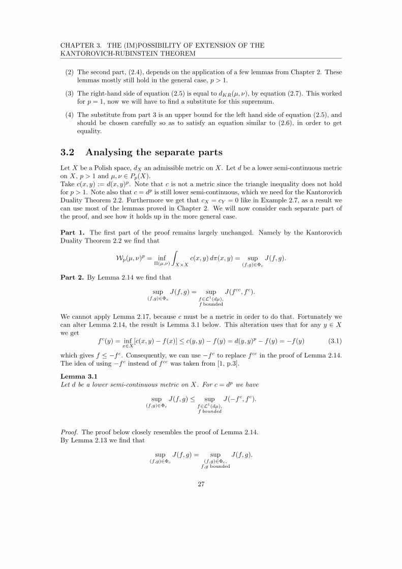
(2) The second part, (2.4), depends on the application of a few lemmas from Chapter 2. Theselemmas mostly still hold in the general case, p > 1.

(3) The right-hand side of equation (2.5) is equal to dKR(µ, ν), by equation (2.7). This workedfor p = 1, now we will have to find a substitute for this supremum.

(4) The substitute from part 3 is an upper bound for the left hand side of equation (2.5), andshould be chosen carefully so as to satisfy an equation similar to (2.6), in order to getequality.

3.2 Analysing the separate parts

Let X be a Polish space, dX an admissible metric on X. Let d be a lower semi-continuous metricon X, p > 1 and µ, ν ∈ Pp(X).Take c(x, y) := d(x, y)p. Note that c is not a metric since the triangle inequality does not holdfor p > 1. Note also that c = dp is still lower semi-continuous, which we need for the KantorovichDuality Theorem 2.2. Furthermore we get that cX = cY = 0 like in Example 2.7, as a result wecan use most of the lemmas proved in Chapter 2. We will now consider each separate part ofthe proof, and see how it holds up in the more general case.

Part 1. The first part of the proof remains largely unchanged. Namely by the KantorovichDuality Theorem 2.2 we find that

Wp(µ, ν)p = infΠ(µ,ν)

∫X×X

c(x, y) dπ(x, y) = sup(f,g)∈Φc

J(f, g).

Part 2. By Lemma 2.14 we find that

sup(f,g)∈Φc


J(f cc, f c).

We cannot apply Lemma 2.17, because c must be a metric in order to do that. Fortunately wecan alter Lemma 2.14, the result is Lemma 3.1 below. This alteration uses that for any y ∈ Xwe get

f c(y) = infx∈X

[c(x, y)− f(x)] ≤ c(y, y)− f(y) = d(y, y)p − f(y) = −f(y) (3.1)

which gives f ≤ −f c. Consequently, we can use −f c to replace f cc in the proof of Lemma 2.14.The idea of using −f c instead of f cc was taken from [1, p.3].

Lemma 3.1Let d be a lower semi-continuous metric on X. For c = dp we have

sup(f,g)∈Φc


J(−f c, f c).

Proof. The proof below closely resembles the proof of Lemma 2.14.By Lemma 2.13 we find that

sup(f,g)∈Φc


J(f, g).

27


Let (f, g) ∈ Φc such that f and g are bounded. Since f is bounded we find by Lemma 2.12 that f c

is integrable, note that this holds for µ, ν ∈ Pp(X), since they are finite. By definition (f, g) ∈ Φcgives for µ-a.e. x ∈ X and ν-a.e. y ∈ Y that f(x) + g(y) ≤ c(x, y), thus g(y) ≤ c(x, y) − f(x).Now by the definition we see that g ≤ f c ν-a.e. so we get J(f, g) ≤ J(f, f c).By (3.1) we get f ≤ −f c which then gives J(f, g) ≤ J(f, f c) ≤ J(−f c, f c). Hence

sup(f,g)∈Φc



J(−f c, f c).

We do not follow the proof of Lemma 2.14 to the end to get equality, since this does not hold.We do not have that (−f c, fc) ∈ Φc, but then we do not need equality in the first place. Notethat this alteration of Lemma 2.14 is possible because for any x ∈ X we have c(x, x) = 0, whichwe use to obtain (3.1). This would not work for any cost function.

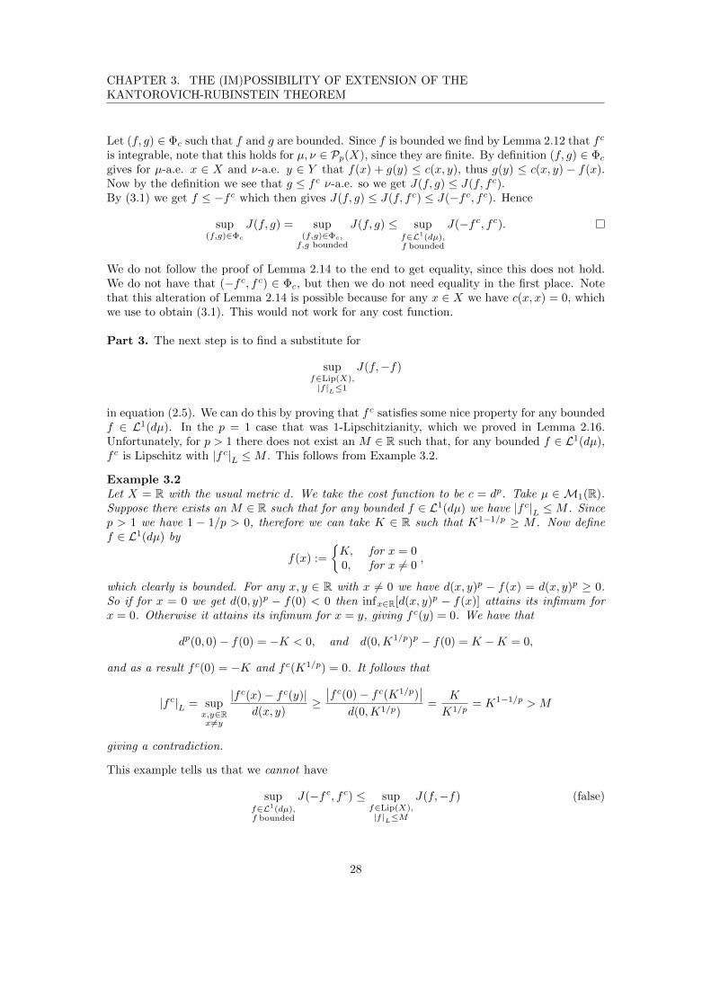
Part 3. The next step is to find a substitute for

supf∈Lip(X),|f |L≤1

J(f,−f)

in equation (2.5). We can do this by proving that f c satisfies some nice property for any boundedf ∈ L1(dµ). In the p = 1 case that was 1-Lipschitzianity, which we proved in Lemma 2.16.Unfortunately, for p > 1 there does not exist an M ∈ R such that, for any bounded f ∈ L1(dµ),f c is Lipschitz with |f c|L ≤M . This follows from Example 3.2.

Example 3.2Let X = R with the usual metric d. We take the cost function to be c = dp. Take µ ∈ M1(R).Suppose there exists an M ∈ R such that for any bounded f ∈ L1(dµ) we have |f c|L ≤M . Sincep > 1 we have 1 − 1/p > 0, therefore we can take K ∈ R such that K1−1/p ≥ M . Now definef ∈ L1(dµ) by

f(x) :=

{K, for x = 00, for x 6= 0

,

which clearly is bounded. For any x, y ∈ R with x 6= 0 we have d(x, y)p − f(x) = d(x, y)p ≥ 0.So if for x = 0 we get d(0, y)p − f(0) < 0 then infx∈R[d(x, y)p − f(x)] attains its infimum forx = 0. Otherwise it attains its infimum for x = y, giving f c(y) = 0. We have that

dp(0, 0)− f(0) = −K < 0, and d(0,K1/p)p − f(0) = K −K = 0,

and as a result f c(0) = −K and f c(K1/p) = 0. It follows that

|f c|L = supx,y∈Rx 6=y

|f c(x)− f c(y)|d(x, y)

≥∣∣f c(0)− f c(K1/p)

∣∣d(0,K1/p)

=K

K1/p= K1−1/p > M

giving a contradiction.

This example tells us that we cannot have


J(−f c, fc) ≤ supf∈Lip(X),|f |L≤M

J(f,−f) (false)

28


for some M ∈ R, like we had in the third step of proof of the Kantorovich-Rubinstein Theorem.Note that without a requirement like |f |L ≤M , this gives no appropriate substitute because

supf∈Lip(X)

J(f,−f)

does not exist by Lemma 1.19, to not even speak of the problems we would encounter in step 4.To prove 1-Lipschitzianity in the p = 1 case, we used Lemma 1.20 to get for any y, y′ ∈ X that

|f c(y)− f c(y′)| ≤ supx∈X|c(x, y)− c(x, y′)| ≤ c(y, y′)

where we could use the triangle inequality since we had c = d a metric. As we discussed, thisproof does not work for c = dp with p > 1. However, we can use a similar argument to provethat f c is locally Lipschitz.

Definition 3.3Let (X, d) be a metric space. The space of locally Lipschitz functions is given by

LocLip(X) := {f : X → R | f : B → R is Lipschitz for any B ⊂ X bounded} .

For any θ > 0 we define for all f ∈ LocLip(X) the constant

|f |L,θ := sup

{|f(x)− f(y)|

d(x, y): x, y ∈ Be(θ), x 6= y

}where we take |f |L,θ = 0 if there exist no x, y ∈ Be(θ) such that x 6= y.

Note that proving for a function f : X → R that f : Be(θ)→ R is Lipschitz for any θ > 0, sufficeswhen proving local Lipschitzianity.

Lemma 3.4Let f ∈ L1(dµ) be bounded. Take m ∈ R such that |f(x)| ≤ m for all x ∈ X.Then f c ∈ LocLip(X) with |f c|L,θ ≤ p(2θ + (2m)1/p)p−1 for any θ > 0.

Proof. Let θ > 0. Take M := θ + (2m)1/p.Let y ∈ Be(θ). We get for all x ∈ [Be(M)]c that

d(x, y) ≥ (2m)1/p, hence c(x, y) ≥ 2m.

This means thatc(x, y)− f(x) ≥ 2m−m = m.

Sincec(y, y)− f(y) = −f(y) ≤ m

we find infx∈X [c(x, y)− f(x)] ≤ m. We may conclude that for any y ∈ Be(θ) we have

f c(y) = infx∈X

[c(x, y)− f(x)] = infx∈Be(M)

[c(x, y)− f(x)].

For any y, y′ ∈ Be(θ) we find by Lemma 1.20 that

|f c(y)− f c(y′)| =

∣∣∣∣ infx∈Be(M)

[c(x, y)− f(x)]− infx∈Be(M)

[c(x, y′)− f(x)]

∣∣∣∣≤ sup

x∈Be(M)

|c(x, y)− c(x, y′)| = supx∈Be(M)

|d(x, y)p − d(x, y′)p| .

29


Let x′ ∈ Be(M). Since the function on R given by z 7→ zp is differentiable on [0,∞) we get bythe Mean Value Theorem that

|d(x′, y)p − d(x′, y′)p| = pcp−1 |d(x′, y)− d(x′, y′)|

for some c ∈ R between d(x′, y) and d(x′, y′). Note that we have d(x′, y) ≤M + θ andd(x′, y′) ≤M + θ since y, y′ ∈ Be(θ) and x′ ∈ Be(M). Hence we find c ≤M + θ, so we get

|d(x′, y)p − d(x′, y′)p| ≤ p(M + θ)p−1 |d(x′, y)− d(x′, y′)| ≤ p(M + θ)p−1d(y, y′).

Since this inequality holds for all x′ ∈ Be(M), we get for y, y′ ∈ Be(θ) that

|f c(y)− f c(y′)| ≤ supx∈Be(M)

|d(x, y)p − d(x, y′)p| ≤ p(M + θ)p−1d(y, y′).

We conclude that f c is locally Lipschitz with, for any θ > 0,

|f c|L,θ ≤ p(M + θ)p−1 = p(2θ + (2m)1/p)p−1.

Remark 3.5: Note that Lemma 3.4 actually also holds for p = 1, and then gives |f c|L,θ ≤ 1 forall θ > 0, i.e. that f c is 1-Lipschitz. Therefore we can view Lemma 3.4 as a generalization ofLemma 2.16.

The bound that Lemma 3.4 provides on |f |L,θ depends on f , because the m is chosen such thatwe have |f(x)| ≤ m for all x ∈ X. We have not found an upper bound for |f c|L,θ, that works for

any bounded f ∈ L1(dµ). Therefore the lemma does not give


J(−f c, fc) ≤ supf∈LocLip(X),|f |L,θ≤M(θ)

J(f,−f) (not proven)

for some M : (0,∞) → R. And even if this were to hold, there would be the problem thatf ∈ LocLip(X) is not necessarily integrable. It would be integrable if M were bounded but thenwe would have f ∈ Lipe(S) with |f |L ≤ supθ>0M(θ), which is impossible by Example 3.2.Despite proving that the f c is locally Lipschitz, we have not found a suitable substitute for theright-hand side of equation (2.5). Possibly, with more time further results may be obtained.

30

Appendix A

Lower semi-continuity

Let X be a topological space.

Definition A.1A function f : X → R is called lower semi-continuous if for every r ∈ R the set f−1((r,∞]) isopen in X.

Remark A.2: Since for any r ∈ R we have that f−1((r,∞]) is open if and only if[f−1((r,∞])

]cis closed we find that f is lower semi-continuous if and only if for every r ∈ R[

f−1((r,∞])]c

= f−1([−∞, r]) = {x ∈ X : f(x) ≤ r}

is closed. This will be used in the proof of Lemma A.6.

The following proposition gives us an alternate definition of lower semi-continuity, in case X ismetrizable with metric d.

Proposition A.3A function f : X → R is lower semi-continuous if and only if for every x ∈ X and ε > 0 thereexists a δ > 0 such that for all y ∈ X satisfying d(x, y) < δ we have f(y) > f(x)− ε.

Proof. Assume f to be lower semi-continuous. Let x ∈ X and ε > 0. Now f−1((f(x),∞]) isopen and contains x. Hence we can take δ > 0 such that Bδ(x) ⊂ f−1((f(x),∞]) meaning thatfor every y ∈ Bδ(x) we have f(y) > f(x) > f(x)− ε.Now assume that for any x ∈ X and ε > 0 we have a δ > 0 such that f(y) > f(x) − ε for ally ∈ X satisfying d(x, y) < δ. Let r ∈ R and consider f−1((r,∞]). Let x ∈ f−1((r,∞]). We willnow find a neighbourhood for x that is contained in f−1((r,∞]) to prove that this set is open.

We define ε := f(x)−r2 > 0. Take δ > 0 such that for all y ∈ Bδ(x) we have f(y) > f(x) − ε.

Then we find

f(y) > f(x)− ε = f(x)− f(x)− r2

=1

2f(x) +

1

2r >

1

2r +

1

2r = r.

This means that Bδ(x) ⊂ f−1((r,∞]), proving that this set is open for any r ∈ R, thus provinglower semi-continuity for f .

The alternative definition provided by Proposition A.3 says that by choosing an appropriateneighbourhood for x ∈ X we can get the value of f to be either arbitrarily close to f(x) (very

31

APPENDIX A. LOWER SEMI-CONTINUITY

much like continuity) or higher than f(x) (making the statement less powerful).

In [9, p.26] it is stated but not proven that for any nonnegative lower semi-continuous functionwe have a nondecreasing sequence of nonnegative uniformly continuous functions that convergespointwise to the lower semi-continuous function. Using the same construction given in [9, p.26]we will prove a slightly stronger statement. Let (X, d) be a metric space.

Lemma A.4Let f : X → [0,∞] be lower semi-continuous. Then there exists a nondecreasing sequence (fn)n∈Nof bounded nonnegative Lipschitz continuous functions such that |fn|L ≤ n and fn → f pointwise.

Proof. We define the sequence (fn)n∈N by

fn(x) := infy∈X

[f(y) + nd(x, y)].

The function fn is well-defined as f and d are bounded below. We will prove that this sequencesatisfies all requirements. Since d ≥ 0 and f ≥ 0 we see that each fn is indeed nonnegative andthat for every x, y ∈ X we have f(y) +md(x, y) ≥ f(y) +nd(x, y) for m ≥ n so we find fm ≥ fn.To prove Lipschitz continuity let x, x′ ∈ X. Let n ∈ N. Then by Lemma 1.20 it follows that

|fn(x)− fn(x′)| =

∣∣∣∣ infy∈X

[f(y) + nd(x, y)]− infy′∈X

[f(y′) + nd(x′, y′)]

∣∣∣∣≤ sup

y∈X|nd(x, y)− nd(x′, y)|

≤ nd(x, x′),

hence fn is Lipschitz with |fn|L ≤ n.Note that for any x ∈ X we have

fn(x) = infy∈X

[f(y) + nd(x, y)] ≤ f(x) + nd(x, x) = f(x)

so we have that fn ≤ f . Let x ∈ X and ε > 0. We will show that there exists an N ∈ Nsuch that fn(x) ≥ f(x) − ε for all n ≥ N . This will imply fn → f pointwise since (fn)n∈N is anondecreasing sequence and fn ≤ f . Since f is lower semi-continuous we get by Proposition A.3that there exists a δ > 0 such that f(y) > f(x) − ε for all y ∈ Bδ(x). Now choose N ∈ N suchthat Nδ ≥ f(x)− ε. Let n ≥ N . For y ∈ Bδ(x) we find

f(y) + nd(x, y) ≥ f(x)− ε+ nd(x, y) ≥ f(x)− ε

since nd(x, y) ≥ 0. For y 6∈ Bδ(x) we have

f(y) + nd(x, y) ≥ f(y) + nδ ≥ nδ ≥ Nδ ≥ f(x)− ε

since f is nonnegative.So for all y ∈ X we get f(y) + nd(x, y) ≥ f(x)− ε. Hence

fn(x) = infy∈X

[f(y) + nd(x, y)] ≥ f(x)− ε

holds for n ≥ N , proving pointwise convergence. Furthermore we can assume this sequence tobe bounded by replacing fn by min(fn, n) which clearly still satisfies all other requirements.

32


In Lemma A.6 we will closely follow the proof of Hing Tong [8]. We say that a space R isperfectly normal if any closed subset of R can be written as the intersection of countably manyopen subsets of R. In [8, Theorem 3] it is proven that R is perfectly normal if and only if everylower semi-continuous function has a nondecreasing sequence of nonnegative and continuousfunctions converging to it. Since every Polish space, or in fact any metric space, is perfectlynormal we can use this result. We adapt the statement and the proof to suit our situation. Wewill need f to be bounded and we will also use the following lemma.

Lemma A.5For a sequence (fn)n∈N of Lipschitz functions satisfying 0 ≤ fn ≤ 1 and |fn|L ≤ n let

g :=

∞∑n=1

1

2nfn.

Then g is Lipschitz continuous and |g|L ≤ 2.

Proof. We get that g is well defined for any x ∈ X since

0 ≤∞∑n=1

1

2nfn(x) ≤

∞∑n=1

1

2n= 1

holds. We find for any x, y ∈ X that

|g(x)− g(y)| =

∣∣∣∣∣∞∑n=1

1

2nfn(x)−

∞∑n=1

1

2nfn(y)

∣∣∣∣∣ =

∣∣∣∣∣∞∑n=1

1

2n[fn(x)− fn(y)]

∣∣∣∣∣≤

∞∑n=1

1

2n|fn(x)− fn(y)| ≤

∞∑n=1

1

2n|fn|L d(x, y)

≤

[ ∞∑n=1

n

2n

]d(x, y) = 2d(x, y).

Hence g is Lipschitz with |g|L ≤ 2.

Lemma A.6Let f : X → [0,∞] be a bounded lower semi-continuous function. Then there exists a nonde-creasing sequence of nonnegative, Lipschitz continuous functions fn such that fn → f pointwise.

Proof. We will go about this step by step.Step 1. First suppose f takes only two different values α and β. Without loss of generality wecan assume α = 0 and β = 1. The set A := {x ∈ X : f(x) = 0} is closed by Remark A.2.For any n ∈ N let

Bn :=

{x ∈ X : d(x,A) <

1

n

}.

We have that the Bn are open and Bn+1 ⊂ Bn holds for any n ∈ N. Moreover, since A isclosed we have that A =

⋂n∈NBn. Define functions gn := [1− nd(x,Bcn)]

+for all n ∈ N. By

Lemma 1.11 we get that gn is Lipschitz continuous with |gn|L ≤ n.By definition gn satisfies 0 ≤ gn ≤ 1 and gn(x) = 1 for x ∈ Bcn. Also, it satisfies gn(x) = 0 forx ∈ A. Namely for x ∈ A we have

d(x,Bcn) = infy∈Bcn

d(x, y) ≥ infy∈Bcn

infx∈A

d(x, y) = infy∈Bcn

d(y,A) ≥ 1

n

33


since for every y ∈ Bcn we have d(y,A) ≥ 1n . Hence, by definition of gn, we find that gn(x) = 0.

Now we define

g :=

∞∑n=1

1

2ngn

which by Lemma A.5 is Lipschitz continuous. Also we have that g(x) = 0 for x ∈ A. Since A isclosed we have for every x 6∈ A that d(x,A) > 0 hence there exists an n ∈ N such that x 6∈ Bn.This gives us that gn(x) = 1, thus we get g(x) 6= 0 for x 6∈ A. Now fn(x) := min(1, ng(x)) gives asequence of nonnegative Lipschitz continuous functions that is nondecreasing and it’s pointwiselimit is f .

Step 2. Now suppose f takes finitely many different values α1 > α2 > ... > αm. In order to usestep 1 we want functions that take only two values. Define for any 1 ≤ i ≤ m− 1 the function

ϕi(x) :=

{αi+1 for x ∈ X such that f(x) ≤ αi+1

α1 for x ∈ X such that f(x) > αi+1.

Then ϕi ≥ f and since f only takes finitely many values we get by construction that

f = min1≤i≤m−1

ϕi. (A.1)

Since f is lower semi-continuous we get by Remark A.2 for any 1 ≤ i ≤ m− 1 that the set{x ∈ X : f(x) ≤ αi+1} is closed. By construction we have that

{x ∈ X : f(x) ≤ αi+1} = {x ∈ X : ϕi(x) ≤ αi+1}.

This implies that {x ∈ X : ϕi ≤ αi+1} is closed for every 1 ≤ i ≤ m−1. Since each ϕi takes onlytwo values we get by Remark A.2 that each ϕi is lower semi-continuous. So by Step 1 we getthat for each 1 ≤ i ≤ m− 1 there exists a sequence (ϕij)j∈N of nonnegative Lipschitz continuousfunctions that is nondecreasing and converges to ϕi pointwise. Let

fn(x) := min1≤i≤m−1

ϕin(x).

Then (fn)n∈N is a nondecreasing sequence of nonnegative and Lipschitz continuous functions byLemma 1.5. For any x ∈ X we have by equation (A.1) that

limn→∞

fn(x) = min1≤i≤m−1

ϕi(x) = f(x).

Step 3. Now we let f : X → [0,∞] be any bounded nonnegative lower semi-continuous function.Since f is bounded we may restrict ourselves to the situation where 0 ≤ f(x) ≤ 1. For anym, p ∈ Z≥0 such that 1 ≤ p ≤ m− 1 we take the set

Amp :=

{x ∈ X :

p+ 1

m≥ f(x) >

p

m

}and for p = 0 we take

Am0 :=

{x ∈ X :

1

m≥ f(x) ≥ 0

}.

For now we fix m ∈ N. Note thatX =

⋃0≤p≤m−1

Amp.

34


What we have done is, we sliced the range [0, 1] into m pieces and for each piece we took thesubset of X that f sends to that piece. This will help us define a function that takes only finitelymany values, in order to use Step 2. Let gm(x) = p/m for x ∈ Amp. By construction thisfunctions takes m values, satisfies 0 ≤ gm ≤ f and is lower semi-continuous since{x ∈ X : f(x) ≤ (p + 1)/m} = {x ∈ X : gm(x) ≤ p/m} is closed for any 0 ≤ p ≤ m − 1 byRemark A.2. Hence, by Step 2, there exists a nondecreasing sequence (gmj)j∈N of nonnegativeLipschitz continuous functions converging pointwise to gm.Since gm converges pointwise to f , we have that gmm converges pointwise to f . We need anincreasing sequence, so for all n ∈ N we take

fn := max1≤i≤n

gii.

We find that fn is Lipschitz continuous by Lemma 1.5. Furthermore the fn are nonnegative andthe sequence is now nondecreasing since from n to n + 1 we just add another function to takethe maximum over. Also (fn)n∈N still converges pointwise to f since gii ≤ f for all i ∈ N. Hencethis sequence satisfies all requirements.

35

Bibliography

[1] Basso, Giuliano. (2015) , A Hitchhiker’s guide to Wasserstein distances.

[2] Billingsley, Patrick. (1999), Convergence of probability measures, second ed. John Wiley &Sons Inc., New York, A Wiley-Interscience Publication.

[3] Bogachev, Vladimir I. (2007), Measure theory, Vol. 2, Springer Berlin Heidelberg.

[4] Burckel, Robert B. & Bauer, Heinz. (2011), Measure and Integration Theory, Berlin,Boston: De Gruyter.

[5] Dudley, Richard M. (1966), Convergence of Baire measures, Stud. Math. 27, 251–268.

[6] Hanin, Leonid G. (1999), An Extension of the Kantorovich Norm, Contemporary Math.Vol. 226.

[7] Hille, Sander C. and Worm, Daniel T.H. (2009), Embedding of semigroups of Lipschitzmaps into positive linear semigroups on Banach spaces generated by measures, Integr. Equ.Oper. Theory 63, 351–371.

[8] Tong, Hing. (1952), Some characterizations of normal and perfectly normal spaces, DukeMath. J. 19, no. 2, 289–292.

[9] Villani, Cedric. (2003), Topics in Optimal Transportation, American Math. Society.

[10] Worm, Daniel T.H. (2010), Semigroups on Spaces of Measures (Doctoral thesis, LeidenUniversity).

36

metrics on spaces of measures

Documents