methods for imaging thick specimens: confocal microscopy, deconvolution, and structured

Topic Introduction

Methods for Imaging Thick Specimens: Confocal Microscopy,Deconvolution, and Structured Illumination

John M. Murray

When a thick specimen is viewed through a conventional microscope, one sees the sum of a sharpimage of an in-focus region plus blurred images of all of the out-of-focus regions. High background,scattering, and aberrations are all problems when viewing thick specimens. Several methods are avail-able to deal with these problems in living samples. These methods can be grouped into three classes:primarily optical (e.g., confocal microscopy, multiphoton microscopy), primarily computational (e.g.,deconvolution techniques), and mixed (e.g., structured illumination) approaches. This articledescribes these techniques, which make it possible to see details within thick specimens (e.g., theinteriors of cells within living tissue) by optical sectioning, without the artifacts associated with phys-ically sectioning the specimen.

BACKGROUND

When a thick specimen is viewed through a conventional microscope, the depth of field (i.e., thedistance between the top and the bottom of the in-focus region at a fixed setting of the focus knob)is <1 µm for the high-numerical-aperture (high-NA) objective lenses that are used for fluorescencemicroscopy. Thus, even when viewing a specimen as thin as 5 µm, 80% of the light may be comingfrom out-of-focus regions. The result will be a low-contrast image, composed of an intensely brightbut very blurred background on which is superimposed the much dimmer in-focus information.

Thick and thin here refer to the thickness of the fluorescent material; overall specimen thicknessper se does not increase the background. However, as the overall specimen thickness increases beyond5–10 µm, other factors begin to degrade the image quality. When the illumination or imaging pathintersects regions of widely different refractive indexes such as small granules or organelles, theircurved surfaces act as microlenses to deflect the light in random directions. The consequence of mul-tiple deflectionsmay be to distort the light path enough to introduce aberrations into the image or evento scatter the light completely out of the field of view.

One way to eliminate the high background, scattering, and aberrations is to slice the thick speci-men into many thin sections, which unfortunately requires fixation, dehydration, and embedding.That approach has limited application to the microscopy of living cells, but fortunately severalother methods work well with living samples. These methods can be grouped into three classes:primarily optical (e.g., confocal microscopy, multiphoton microscopy), primarily computational(e.g., deconvolution techniques), and mixed (e.g., structured illumination) approaches.

Adapted from Live Cell Imaging, 2nd edition (ed. Goldman et al.). CSHL Press, Cold Spring Harbor, NY, USA, 2010.

© 2011 Cold Spring Harbor Laboratory PressCite this article as Cold Spring Harbor Protoc; 2011; doi:10.1101/pdb.top066936

1399

Cold Spring Harbor Laboratory Press on April 10, 2019 - Published by http://cshprotocols.cshlp.org/Downloaded from

http://cshprotocols.cshlp.org/

http://www.cshlpress.com

Which Method to Use?

A systematic approach to choosing the best method is described at the end of the article, but a fewintroductory comments may be useful here. These methods are discussed here because theyaddress problems encountered in imaging thick specimens such as living cells. For routine qualitativeobservation of relatively thin specimens (<3 µm), it will probably bemuch quicker and less frustratingto avoid them all and use conventional (wide-field) microscopy. However, there are a few situations inwhich the benefits of these more complexmethods are important enough, even for a thin specimen, towarrant the extra cost, inconvenience, and time.

The most common application to thin specimens is when intrinsic contrast is very low, so that anyloss of contrast, even the minimal decrease because of a small amount of out-of-focus light, compli-cates interpretation of the data. In this situation, all of these methods can usually improve contrast forany sample thicker than�2 µm. Another common application is to enable accurate measurement ofthe amount of a fluorescent component present in a cell, a task in which deconvolutionmethods excel.Finally, in the case in which a modest enhancement of resolution would change the interpretation ofthe data, then confocal, deconvolution, and some of the structured illumination methods are capableof delivering a small improvement over a conventional microscope. However, for most thin samples,the small improvement will not be worth the large extra effort. For very thin samples, <1 µm, quiteextraordinary improvements in resolution are possible using several different modes of structuredillumination (Heintzmann and Ficz 2007), but unfortunately these are not yet applicable toliving cells.

For thicker objects that produce a moderate amount of out-of-focus light (typically 5–30 µm), anyof the methods discussed here, and also multiphoton microscopy, should give a dramatically betterresult than a conventional microscope.When the sample is living (i.e., photobleaching and phototoxi-city constrain exposure) and the signal is weak or the contrast is low, methods that must use photo-multipliers for detection (e.g., point-scanning methods, confocal or multiphoton) have a severehandicap compared with methods that can use charge-coupled device (CCD) cameras (e.g., decon-volution, disk- or array-scanning confocal, structured illumination), because of the much higherquantum efficiency of CCDs. However, with very thick specimens that produce an overwhelmingamount of out-of-focus light, only point-scanning (confocal or multiphoton) microscopy will givea satisfactory result.

How much is a moderate amount of out-of-focus light? Typically in such a specimen, the imageseen through a conventional microscope will be too blurred to be useful, but one will be able to locatethe region of interest and at least roughly set the focus level. Thus it is possible to locate the area to beimaged by visual observation, although the image will be too blurred to discern details. On the otherhand, if the view through a conventional microscope is virtually featureless, giving no landmarks forchoosing the appropriate area or for setting the focus, then currently the only choices arepoint-scanning confocal or multiphoton microscopy. These two methods can produce extremelyuseful images from outrageously bad specimens. However, from these very thick specimens, it isnot realistic to expect a final image quality comparable to the best that a conventional microscopeproduces with a thin specimen, for reasons that we will consider in this article.

DECONVOLUTION METHODS

The goal of these techniques is to improve the images of thick objects by computationally removingthe out-of-focus blur. The strategy is to calculate the structure of a hypothetical object that could haveproduced the observed partially focused image. The calculation is based on fundamental optical prin-ciples—in particular, a quantitative understanding of the effects of defocus—and may also take intoaccount prior information or guesses about the specimen. The method commonly used is to refineiteratively an initial guess at the true object until the estimated image (i.e., the estimated object appro-priately blurred by the effects of defocus) corresponds to the actual observed image.

1400 Cite this article as Cold Spring Harbor Protoc; 2011; doi:10.1101/pdb.top066936

J.M. Murray




Optical Principles

Successful application of these techniques requires an appreciation of how an image is formed by amicroscope and what happens to an image when the lens is defocused. For this purpose, it ishelpful to introduce the twin concepts of point-spread function (PSF) and contrast-transfer function(CTF). Both of these concepts describe the relationship between a real object and the image that isformed of it by an optical system. The PSF describes this relationship in terms of the image of avery small object, effectively a single point. Although the microscope can see objects as small as asingle molecule, its limited resolution prevents the image from accurately portraying the size ofvery small objects, no matter what magnification is applied.

An illustration of this phenomenon is given in Figure 1. Notice that below a certain object size,images of every object appear the same. Increasing the magnification does not help; the image canbemade larger, but not sharper. This limiting image is called an Airy disk, after the British astronomerG.B. Airy who first recognized its significance in 1834. Notice that, for this microscope, the Airy disk isnot quite a perfect circle. The three smallest beads all appear to be slightly elliptical, with a weaker tailextending toward the upper right. Now, one might have been willing to concede that the manufactur-ing process somehow makes ellipsoids instead of spheres for all beads below a certain size, but itstrains credulity to postulate that by coincidence, all of the beads that I photographed just happenedto be oriented in exactly the same direction! In fact, electron microscopy shows that the beads arenearly perfect spheres. As Airy was the first to point out, the shape of this limiting image providesno information about the shape of the object—the Airy disk is an intrinsic property of the opticalsystem itself. The Airy disk reveals that the image of a pointlike object is not a single point but isspread into a fuzzy disk. From this spreading is derived the more informative name for the Airydisk, which is the PSF. The PSF is often used as a means of quantitatively characterizing the perform-ance of an imaging system.

The grating images in Figure 1 show that the size of the PSF sets the resolving power of an opticalsystem. An optical system forms an image by substituting its PSF for every point in the object and thensums all of these PSFs to make the image. The width of the PSF determines how far apart two points inthe object must be to avoid being smeared together in the image. If the PSF of the optical system isbroad, two points will have to be rather well separated to prevent the overlap of the two corresponding

FIGURE 1. Epifluorescencemicroscope images of eight beads of known, decreasing size. The images of the fluorescentbeads are shown in green, all adjusted to have the same maximum brightness. The actual brightness varied by�1000-fold. The true diameter of each bead is given above its image, and the diameter measured from the imageis listed below it. The four smallest beads are shown at two different magnifications. The apparent diameters measuredin the image are slightly larger than the true diameters, and the apparent diameters are the same for the three smallestbeads, even though their true diameters differ by more than fivefold. These three images reveal the PSF of this micro-scope. The images in the upper right corner, obtained with the same microscope setup, show the appearance of threegratings with spacings of 0.29, 0.25, and 0.20 µm between the white bars. Notice that the contrast between the blackand white bars decreases as the spacing gets smaller. In the actual object, the grating contrast is the same for all threescales. The bead images in the upper row are displayed at the same magnification as the gratings.

Cite this article as Cold Spring Harbor Protoc; 2011; doi:10.1101/pdb.top066936 1401

Methods for Imaging Thick Specimens




PSFs in the image. If their PSFs overlap extensively, then the two points will appear to be just a singlepoint, smeared into a mushy average just like the lines in the image of the 0.2-µm grating. The smear-ing process is described mathematically as a convolution of the PSF with the object to produce theimage. A good way to visualize this convolution is to imagine painting a picture of the object usinga paintbrush with a tip the size of the PSF.

To take a concrete example, suppose that I had chosen not an individual 0.04-µm bead for theexperiment in Figure 1 but instead inadvertently picked a pair of 0.04-µm beads separated by 0.08µm, twice their own diameter. This pair would still be a smaller object than the single 0.22-µmbead, and their joint image would have the same shape as any of the three limiting images inFigure 1. In other words, 0.08 µm is well below the resolution of this microscope. It is importantto realize however, that the Airy disk for the pair of beads would be twice as bright as the Airy diskfrom a single bead. In other words, the imaging process is a linear operation. The total intensity inan image of (A + B) is exactly the sum of the total intensity in an image of A plus the total intensityin an image of B.

A single number is often quoted for the resolving power of a microscope, such as the Rayleigh cri-terion, which is the radius of the Airy disk, given numerically by 0.6 λ/NA for incoherent imaging as influorescence microscopy, in which NA is the numerical aperture of the objective lens and λ is thewavelength of light that forms the image. However, using a single number for the resolving poweris somewhat misleading because there is no sharp cutoff. As their size approaches the resolution ofthe imaging system, small details do not suddenly disappear. Instead, their contrast in the imagebecomes a smaller and smaller fraction of their true contrast in the object, until finally the image con-trast approaches the size of the random fluctuations because of noise, and they then become invisible.The images of the gratings in Figure 1 show this progressive loss of contrast with decreasing size.

A complete description of the resolving power of an optical system thus requires informationabout the variation of contrast with size or, more precisely, the variation in the ratio of image contrastto object contrast as a function of size. The PSF actually contains this information, but it is revealedmore clearly in its twin, the CTF. This function describes the extent to which contrast variations inthe object are faithfully replicated in the image. Perfect contrast transfer means that image contrastequals object contrast. The CTF is usually expressed as a ratio, so that perfect contrast transfermeans that the CTF has a value of 1.0. In the real world, things are less than perfect, and the CTFis always <1.0.

It is reasonable to expect that information about some features of the object might be transferredinto the image more faithfully than others. For instance, the image may be a nearly perfect represen-tation of the large-scale features of the object but contain much less information about the very smal-lest details. This will always be true for images obtained from an optical microscope because onecannot see clearly those details of the object that are small compared with the wavelength of light(i.e., details on the scale of the PSF). Thus the CTF is a function of the size of the feature beingobserved (Fig. 2, left). Normally the CTF is shown in a graphical form, plotting the ratio of image con-trast to object contrast (vertical axis) against the reciprocal of size (i.e., spatial frequency). The CTF issimply a different representation of the same information given by the PSF of an optical system.Math-ematically, the CTF and the PSF are related as Fourier-transform pairs.

Fundamentally then, when we speak of image resolution, we are, in fact, making a statement aboutimage contrast at small spacings—alternatively, to be precise, about the ratio of image to object con-trast at small spacings. Thus there is always an interaction between image contrast, imagesignal-to-noise (SNR) ratio, and image resolution, even though it is sometimes convenient to thinkof these as independent properties. What we normally refer to as visibility is determined by allthree of those parameters and also by properties of the display system and the observer. Because ofthese subjective elements, visibility is not the last word—often one can extract much useful infor-mation concerning features that, by eye, are invisible.

The example of a typical good microscope CTF and PSF shown on the left-hand side of Figure 2represents the case in which the specimen is thin and lies exactly in the focal plane of the objective lens.In fact, the CTF and PSF are three-dimensional (3D) functions. Their third dimension is revealed by


J.M. Murray




comparing image to object when the object is displaced vertically from the focal plane of the lens. Asthe focus changes, a very surprising thing happens: Concentric rings appear in the PSF, and the CTFdevelops ripples, in some regions becoming negative. This means that for some features of the object,the image will have reversed contrast. For features in the size range corresponding to these negativeoscillations of the CTF, dark parts of the object will appear bright in the image and vice versa (Fig. 2,right). As the degree of defocus increases, the CTF becomes increasingly oscillatory, with the contrastreversals affecting ever larger features in the image.

The image of a small fluorescent bead (i.e., the PSF) develops concentric rings as the lens movesaway from focus (Fig. 2, top right). Changing the focus of the lens means that the 3D PSF is viewed atdifferent levels along the optical axis. A vertical slice of the complete computed (Born and Wolf 1999,p. 489) 3D PSF, viewed from the side, is shown in Figure 3.

It surprises most people that microscopes can produce such wildly incorrect images as depicted inFigures 2 (right) and 3. A striking example is shown in Figure 4, but the same effect can easily beobserved on almost any specimen. In bright field, a small high-contrast feature such as a small dustparticle or a scratch shows the contrast-reversal phenomenon clearly. Using a good dry oroil-immersion lens, carefully focus up and down by a small distance on either side of the correctfocus, and you will see the particle oscillate from bright to dark and back again. If you can controlthe focus carefully enough, you may be able to find the position, halfway between a bright and adark oscillation, where the particle becomes practically invisible (i.e., CTF� 0 for details of thissize). Evidently, some care is required in interpreting microscope images. How can you tell whichis the correct appearance?

To reiterate, a microscope substitutes its 3D PSF for each point in the 3D object and then sums allof those innumerable PSFs to give the final 3D image. The mathematical operation called convolutionprecisely describes this substitute and sum process. The distribution of intensities in the 3D image isthe result of convolving the object-intensity distribution with a 3D PSF. The 3D PSF is an intrinsicproperty of the optical system and does not depend on the object.

FIGURE 3. Vertical sections through the 3D PSFs calculated forlenses of two different NAs. The contrast has been greatlyenhanced to show the weak side lobes (which are the ringsof the Airy disk, viewed edge on). The small insets show thePSFs at their true contrast level. Note that vertical smearing(proportional to NA2) is much more strongly affected by thelens NA than is lateral smearing (proportional to NA).

FIGURE 2. (Left) Schematic of some CTFs and the corresponding PSFs (object-image pairs for a very small object). (A) Aperfect (impossible) microscope; (B) a typical good microscope; (C ) a poor or improperly used microscope. Thedashed line lies at a relative contrast of 25%, corresponding to the Rayleigh criterion for the resolving power of amicro-scope. (Right) Images of a tiny object from a microscope at two different values of defocus reveal the 3D nature of thePSF and CTF. Objects in some size ranges appear to change from black towhite or vice versa as the focus level changesbetween the two indicated values. An example of this contrast reversal in a transmitted light image is shown inFigure 4.






Deconvolving Wide-Field Microscope Images

The 3D PSF (or equivalently, the 3D CTF) contains all the information one would need to predict theappearance of a known object when viewed through the corresponding optical system for any choiceof focus. However, our problem is the converse of this. We know the appearance (i.e., the image), butwe would like to know the real structure of the object. It is, in principle, possible to go backward in aone-step calculation from the observed appearance to the actual structure using the mathematicalprocedure of deconvolution. In practice, for realistic SNRs, a much better approach is to carry outthis calculation in a multistep, iterative fashion. To see how the iterative deconvolution procedureworks, imagine that the 3D object is made up of a stack of discrete two-dimensional (2D) planes. Nor-mally the data will also be a stack of 2D-image planes, collected by changing the fine focus of themicroscope by a small increment between successive images. To illustrate the iterative calculation,we will describe the steps for calculating one plane, say number 5, of an object that is nine planesthick (Fig. 5).

Consider plane number 5 of the observed stack of images (Fig. 5). When this image was recorded,what the detector saw was the sum of an in-focus view of object plane number 5, plus a view of objectplane number 6 blurred by one increment of defocus, plus object plane number 4 blurredby one increment of defocus in the opposite direction, plus plane numbers 7 and 3 blurred byplus and minus two increments of defocus, respectively, and so forth. To simulate this process

FIGURE 4. Contrast reversal because of defocus. (Left) A bright-field image of a diatom taken through a conventionalmicroscope using a 60× (NA = 1.4) objective. (Right) An enlargement of a small portion of the image on the left,showing contrast reversals because of changing amounts of defocus. The diatom shell is curved, being thinner atthe edges. As a result, the distance from the lens to the surface of the diatom varies; that is, the view includes arange of defocus values. Over this range, the CTF changes sign several times: From left to right, the holes changefrom black to white, to black again, and finally to white on the right-hand edge. The white rectangle indicates anarrow band midway between a black and a white hole region where the contrast of the holes is low; that is, theCTF is nearly 0 for structures of this size at this value of defocus.

FIGURE 5. A simplified illustration of how one plane in the microscopic image of a thick object is formed. The processcan be thought of as adding the in-focus image of one object plane to the images of neighboring object planes viewedat different amounts of defocus. For clarity, the process is illustrated for only two neighbors on each side of the in-focusplane. In reality, each image plane receives contributions from all object planes.


J.M. Murray




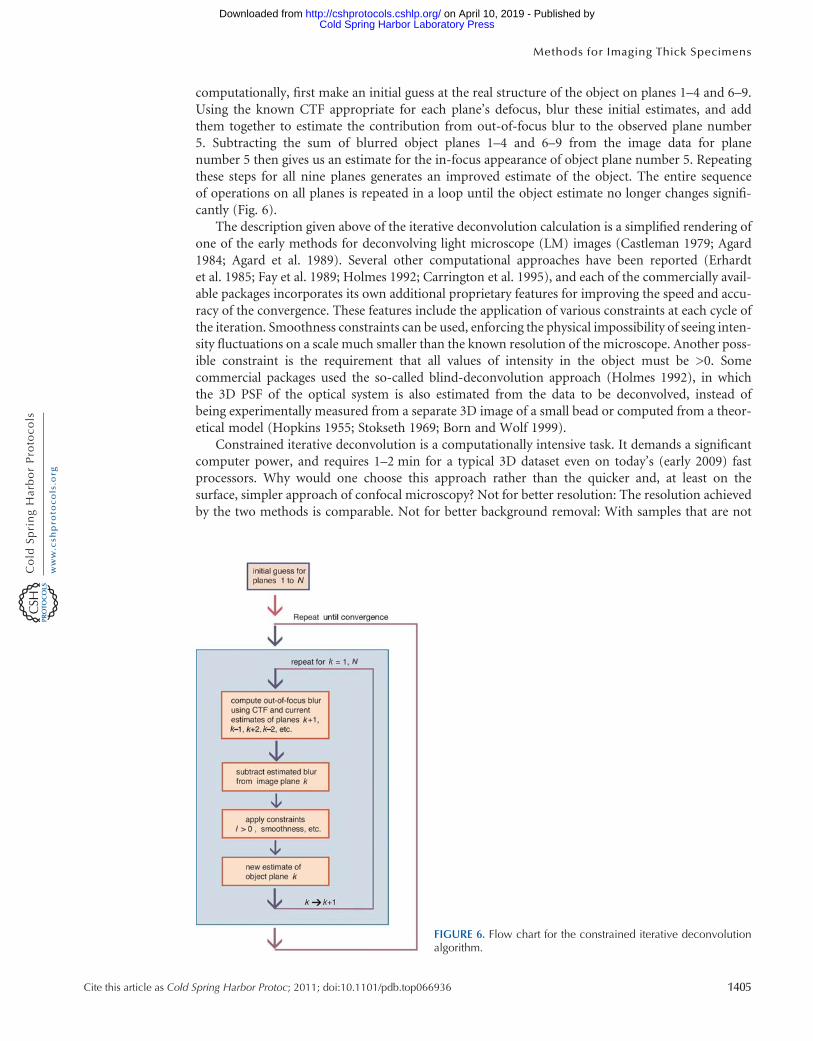
computationally, first make an initial guess at the real structure of the object on planes 1–4 and 6–9.Using the known CTF appropriate for each plane’s defocus, blur these initial estimates, and addthem together to estimate the contribution from out-of-focus blur to the observed plane number5. Subtracting the sum of blurred object planes 1–4 and 6–9 from the image data for planenumber 5 then gives us an estimate for the in-focus appearance of object plane number 5. Repeatingthese steps for all nine planes generates an improved estimate of the object. The entire sequenceof operations on all planes is repeated in a loop until the object estimate no longer changes signifi-cantly (Fig. 6).

The description given above of the iterative deconvolution calculation is a simplified rendering ofone of the early methods for deconvolving light microscope (LM) images (Castleman 1979; Agard1984; Agard et al. 1989). Several other computational approaches have been reported (Erhardtet al. 1985; Fay et al. 1989; Holmes 1992; Carrington et al. 1995), and each of the commercially avail-able packages incorporates its own additional proprietary features for improving the speed and accu-racy of the convergence. These features include the application of various constraints at each cycle ofthe iteration. Smoothness constraints can be used, enforcing the physical impossibility of seeing inten-sity fluctuations on a scale much smaller than the known resolution of the microscope. Another poss-ible constraint is the requirement that all values of intensity in the object must be >0. Somecommercial packages used the so-called blind-deconvolution approach (Holmes 1992), in whichthe 3D PSF of the optical system is also estimated from the data to be deconvolved, instead ofbeing experimentally measured from a separate 3D image of a small bead or computed from a theor-etical model (Hopkins 1955; Stokseth 1969; Born and Wolf 1999).

Constrained iterative deconvolution is a computationally intensive task. It demands a significantcomputer power, and requires 1–2 min for a typical 3D dataset even on today’s (early 2009) fastprocessors. Why would one choose this approach rather than the quicker and, at least on thesurface, simpler approach of confocal microscopy? Not for better resolution: The resolution achievedby the two methods is comparable. Not for better background removal: With samples that are not

FIGURE 6. Flow chart for the constrained iterative deconvolutionalgorithm.






outrageously thick, the two methods are approximately equal in their ability to remove the out-of-focus background light that degrades contrast. Where deconvolution plus wide-field microscopy isclearly superior to confocal microscopy is in the quality of the image data, measured as SNR(Murray et al. 2007).

There are several reasons why this is so, and these will be discussed later in the Interpreting theResults section of this article. The point to stress here is that with living samples, higher SNRbecomes a top priority. If one is examining only fixed cells by, for example, labeling with antibodies,then quantitative measurements of the fluorescence intensity are not usually worthwhile because ofthe huge uncertainties inherent in immunocytochemical detection. However, it is now possible toimage protein molecules in living cells. Suddenly, the types of questions one can ask have changedbeyond recognition because the molecules can be directly counted (Femino et al. 1998). The yieldof information from live cell experiments can be enormously increased if the SNR in the imagesis high enough to extract reliable quantitative estimates of fluorophore distribution (Swedlowet al. 2002).

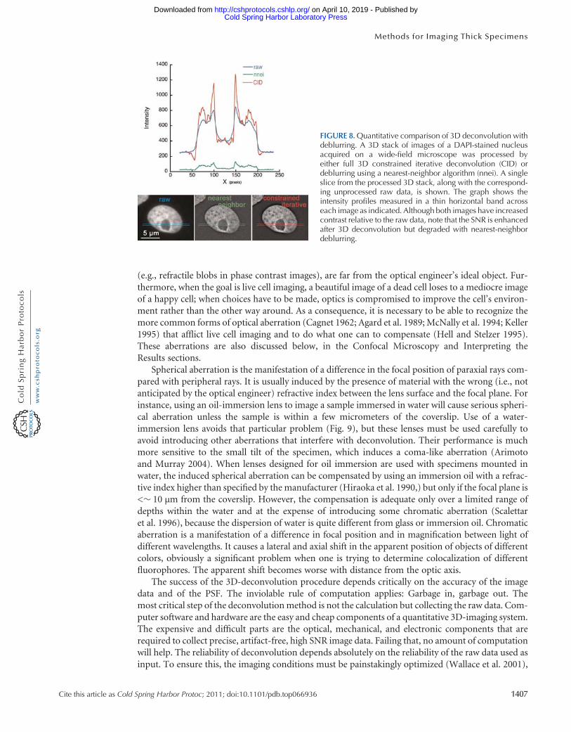
Having said that, there are occasions, particularly if real-time evaluation is needed, when aquick-and-dirty contrast enhancement procedure is useful. For this purpose, there are severalother less rigorous computational methods for enhancing the contrast in images that have beendegraded by high background. It is very important to distinguish between true 3D deconvolutionas described above, a mathematically linear operation, and the several varieties of fast, simple, deblur-ring algorithms (nearest neighbor, multineighbor, unsharp masking), which are fundamentally 2Doperations, and mathematically nonlinear, although often cosmetically quite effective. Only thelinear operation of 3D deconvolution restores image intensities so that they correspond quantitativelyto the intensity distribution in the object. In doing so, this operation increases the SNR of the data(Fig. 7), and the output images are appropriate for all forms of quantitative measurement. The math-ematically nonlinear deblurring algorithms can make the image look better, but the SNR is oftendegraded (Fig. 8). The output data from these nonlinear procedures may be acceptable for distancemeasurements on high-contrast objects, but are not usable for quantitative measurements of fluoro-phore distribution.

Practical Aspects and Tips for Generating Reliable Images

A superb guide to the practical aspects of deconvolving LM images has been published (Wallace et al.2001). Anyone interested in using deconvolution methods will find that guide to be a gold mine ofuseful information. There is neither need nor space to repeat all of that information here, but abrief mention of some of the optical challenges in live cell imaging will be useful for the later discus-sion of confocal microscopy.

Modern objective lenses are nearly perfect when used under the conditions for which they weredesigned. Unfortunately, living cells, with all their structural variation and optical inhomogeneities

FIGURE 7.Deconvolution of wide-field microscope images of the parasite Toxoplasma gondii expressing YFP tubulin(Swedlow et al. 2002). (Left) One focal plane near the plasma membrane from a 3D stack of raw images of YFP fluor-escence in several living parasites. (Middle) The same focal plane after processing of the 3D stack by constrained itera-tive deconvolution. Microtubules are clearly visible as bright striations. (Right) A plot of the change in intensity alongthe dashed lines in the raw data and in the data after deconvolution. Deconvolution greatly improved the SNR byrestoring the out-of-focus light to its proper location. (Specimen kindly provided by Dr. Ke Hu, Indiana University,Bloomington. Images and deconvolution courtesy of Paul Goodwin, Applied Precision Inc.)


J.M. Murray




(e.g., refractile blobs in phase contrast images), are far from the optical engineer’s ideal object. Fur-thermore, when the goal is live cell imaging, a beautiful image of a dead cell loses to a mediocre imageof a happy cell; when choices have to be made, optics is compromised to improve the cell’s environ-ment rather than the other way around. As a consequence, it is necessary to be able to recognize themore common forms of optical aberration (Cagnet 1962; Agard et al. 1989; McNally et al. 1994; Keller1995) that afflict live cell imaging and to do what one can to compensate (Hell and Stelzer 1995).These aberrations are also discussed below, in the Confocal Microscopy and Interpreting theResults sections.

Spherical aberration is the manifestation of a difference in the focal position of paraxial rays com-pared with peripheral rays. It is usually induced by the presence of material with the wrong (i.e., notanticipated by the optical engineer) refractive index between the lens surface and the focal plane. Forinstance, using an oil-immersion lens to image a sample immersed in water will cause serious spheri-cal aberration unless the sample is within a few micrometers of the coverslip. Use of a water-immersion lens avoids that particular problem (Fig. 9), but these lenses must be used carefully toavoid introducing other aberrations that interfere with deconvolution. Their performance is muchmore sensitive to the small tilt of the specimen, which induces a coma-like aberration (Arimotoand Murray 2004). When lenses designed for oil immersion are used with specimens mounted inwater, the induced spherical aberration can be compensated by using an immersion oil with a refrac-tive index higher than specified by the manufacturer (Hiraoka et al. 1990,) but only if the focal plane is<� 10 µm from the coverslip. However, the compensation is adequate only over a limited range ofdepths within the water and at the expense of introducing some chromatic aberration (Scalettaret al. 1996), because the dispersion of water is quite different from glass or immersion oil. Chromaticaberration is a manifestation of a difference in focal position and in magnification between light ofdifferent wavelengths. It causes a lateral and axial shift in the apparent position of objects of differentcolors, obviously a significant problem when one is trying to determine colocalization of differentfluorophores. The apparent shift becomes worse with distance from the optic axis.

The success of the 3D-deconvolution procedure depends critically on the accuracy of the imagedata and of the PSF. The inviolable rule of computation applies: Garbage in, garbage out. Themost critical step of the deconvolutionmethod is not the calculation but collecting the raw data. Com-puter software and hardware are the easy and cheap components of a quantitative 3D-imaging system.The expensive and difficult parts are the optical, mechanical, and electronic components that arerequired to collect precise, artifact-free, high SNR image data. Failing that, no amount of computationwill help. The reliability of deconvolution depends absolutely on the reliability of the raw data used asinput. To ensure this, the imaging conditions must be painstakingly optimized (Wallace et al. 2001),

FIGURE 8.Quantitative comparison of 3D deconvolution withdeblurring. A 3D stack of images of a DAPI-stained nucleusacquired on a wide-field microscope was processed byeither full 3D constrained iterative deconvolution (CID) ordeblurring using a nearest-neighbor algorithm (nnei). A singleslice from the processed 3D stack, along with the correspond-ing unprocessed raw data, is shown. The graph shows theintensity profiles measured in a thin horizontal band acrosseach image as indicated. Although both images have increasedcontrast relative to the raw data, note that the SNR is enhancedafter 3D deconvolution but degraded with nearest-neighbordeblurring.






and there are several important preprocessing steps that must be performed to correct various artifactstypically present in 3D-epifluorescence image data (Hiraoka et al. 1990; Scalettar et al. 1996; McNallyet al. 1999; Markham and Conchello 2001).

Limitations

As with any other technique, limitations to the use of deconvolution methods exist: Some specimensare unsuitable, and some suitable specimens challenge the currently available computational methods.One straightforward limitation is the need for a certain minimal SNR in the input data. All of thealgorithms have the potential for amplifying noise. If the input signal is too noisy (i.e., the noise islarge compared with the contrast between signal and background), then naturally the algorithmswill fail, and the output will be meaningless. Effectively, this limits deconvolution methods to speci-mens in which the ratio of background fluorescence to in-focus signal is no greater than �20:1(Murray et al. 2007).

Other limitations are not intrinsic to the method itself but are imposed by limited computationalresources. For instance, the algorithms assume that the PSF of the optical system is the same for allpoints in the field of view (shift invariance) because the computations required to take account ofa spatially variant PSF are not feasible for most applications (McNally et al. 1994). However, it iseasy to show experimentally that this assumption is routinely violated in images of typical large(i.e., nonyeast) eukaryotic cells. Incorporating a measurement of local optical inhomogeneitiesbased on differential interference contrast (DIC) imaging into an algorithm that allows for space-variant deconvolution is one promising approach to deal with this problem (Kam et al. 2001).

Another assumption that is incorporated into most algorithms (e.g., in smoothing filters that areused to constrain the intermediate calculations) is that the data are stationary in a statistical sense,which would require that the power spectrum be the same for every small region of the image.Obviously, this is far from true for any biological sample, particularly when the image records fluor-ophore distribution. Again, this assumption is not a necessary feature of the restoration algorithms

FIGURE 9. Effect of imaging depth on lens performance. Three-dimensional stacks of images of small fluorescent beadsimmersed in water were acquired, using an oil-immersion objective lens, a water-immersion objective, and an objec-tive designed for use with a silicone oil as the immersion medium (refractive index�1.4). The graph shows the inten-sity of the bead image in each focal plane of the 3D stacks from three beads located at different distances from thecoverslip surface (at depth = 0). For objects located immediately adjacent to the coverslip, the oil-immersion lensgives a brighter signal and sharper axial response than the other lenses. However, its performance is rapidly degradedby spherical aberration with increasing depth, whereas the other two objectives are less sensitive, so that at depthscorresponding to typical eukaryotic cells the performance ranking is reversed.


J.M. Murray




(Castleman 1996, pp. 398–403) but a simplification to reduce the computational load. The practicalconsequence of violating this assumption is that small features can become unstable after a number ofiterations, suddenly disappearing from the calculated result even though they may be present in theraw data.

A disadvantage of wide-field/3D deconvolution compared with, for instance, spinning-disk con-focal imaging is the need to obtain a 3D stack of images even though the feature of interest may beconfined to a single optical section. Phototoxicity caused by the extra exposure needed for the 3Dstack may limit the overall length of time-lapse studies and may make the experiment impossible iffast processes are being studied. Even when the processes under study are relatively slow, such thatan interval of many minutes between time points is adequate, cell movement on the timescale ofseconds can nevertheless make it very difficult to acquire 3D data for deconvolution. An exampleis shown in Figure 10. Although no rapid processes were under study in that experiment, neverthelessthe 2–3 sec required for acquisition of a 3D stack of images proved to be too long, because cell move-ments during the acquisition made reliable deconvolution impossible.

Protection from being misled by these artifacts is of course purchased simply and in the same coinas for any other experimental undertaking: Onemust design and carry out sensible controls and repeatthe experiment using independent methods and different conditions. Notwithstanding these minordifficulties, for suitable specimens, deconvolution of images from a wide-fieldmicroscope is a tremen-dously powerful technique that produces images of diffraction-limited resolution with less photo-bleaching and phototoxicity than any other method (Murray et al. 2007). It is an invaluablemethod that becomes increasingly important with the rapid progress in visualizing gene productsin living cells.

CONFOCAL MICROSCOPY

The goal of this method is to improve imaging of thick objects by physically removing the out-of-focuslight before the final image is formed (Minsky 1961; Petran et al. 1968; Brakenhoff et al. 1979; Carlssonet al. 1985; Amos et al. 1987). The method takes advantage of differences in the optical path followedby in-focus and out-of-focus light, selectively blocking the latter while passing the former on tothe detector.

FIGURE 10.Movement artifacts in 3D image acquisition. The top row shows three adjacent planes from a stack of 17focal planes of T. gondii expressing a GFP fusion protein that highlights the conoid and other structures. Small move-ments, difficult to appreciate in single images but obvious when the stack is replayed as a movie sequence, occurredduring acquisition of planes 6, 7, and 8. Overlaying the three planes as red, green, and blue (RGB) channels of an RGBimage reveals the movement of one conoid (red arrow). After deconvolution, viewing the 3D reconstruction at anoblique angle reveals the distortion (red arrow; jagged profile of the conoid, which is actually round).






Optical Principles

Confocal microscopes differ from conventional (wide-field) microscopes because they do not “see”out-of-focus objects. In a confocal microscope, most of the out-of-focus light is excluded from thefinal image, greatly increasing the contrast and hence the visibility of fine details in the specimen.Figure 11 shows a comparison of images of the same thick specimen viewed by both wide-fieldand confocal microscopes. Figures 12 and 13 give schematics of the operating principle. On the left-hand side of Figure 12 is a wide-field microscope. A light source, in conjunction with a condenser,distributes light uniformly across the area of the specimen under observation. The diagram illustratesthe paths followed by light arising from the specimen, passing up through the objective lens and even-tually (ignoring some intermediate lenses that need not concern us here) reaching a detector of somesort: film, video camera, or retina. Three paths are shown, corresponding to light arising from threelocations in the sample. The first location is in the center of the field of view and in the focal plane ofthe objective lens. The heavy dashed lines are the limits of the bundle of light rays that contribute tothe image from this point. Similarly, the lighter dashed lines mark the rays from a second point in thesame plane but displaced horizontally from the first point. Finally, light (the dotted lines), is comingfrom a third point located below the first point (i.e., from an out-of-focus plane). The light from thisthird point contributes to the blurred background, which we wish to eliminate from the image.

The right-hand side of Figure 12 shows how this is done, simply by adding a pinhole aperture tothe wide-field microscope. Notice that behind the objective lens, all of the light rays are broughttogether at a crossover point, the location of the intermediate image plane of the microscope. Nor-mally, the microscope oculars are focused on this plane to form the final fully magnified image.

FIGURE 11. Images of a thick fluorescent specimen from a confocal and a conventional microscope. The sample is achick embryo stained with propidium iodide and antibody against the carboxy-terminal glutamic-acid form ofα-tubulin (fluorescein isothiocyanate [FITC] label). (Top left) Low-magnification, wide-field phase-contrast image ofthe entire embryo. The sample is �0.5-mm thick and contains a high density of refractile globules that scatter lightefficiently. (Top right) Phase-contrast image at the same magnification as the fluorescence image. (Middle row) Con-ventional epifluorescence images showing (left) propidium iodide and (right) glu-tubulin distribution. The largeamount of out-of-focus light severely reduces contrast. (Bottom left) Optical section obtained by confocal microscopyof exactly the same field and focal plane as the middle row. (Bottom right) Higher-magnification confocal view of aportion of the same field. Mitotic nuclei with condensed chromatin can be readily identified. (Dotted white ellipse)Bundles of tubulin are also seen. The mitotic spindle in these cells is formed predominantly with the tyrosinylatedform of α-tubulin and hence is not seen. (Sample kindly provided by Dr. Camille DiLullo, Philadelphia College ofOsteopathic Medicine.)


J.M. Murray




The location of this crossover plane along the vertical axis of the microscope is different for differentlight rays, depending on the distance of the corresponding point in the specimen from the front of theobjective lens. The crossover point for light rays from the illustrated out-of-focus plane (dotted lines)is below that for rays from the in-focus plane (dashed lines). As illustrated, a pinhole aperture at the

FIGURE 13. A typical laser-scanning confocal microscope. The instrument consists of a conventional fluorescencemicroscope (enclosed in the lower shaded rectangle) to which has been attached a confocal-scanning unit (uppershaded rectangle) comprising a pair of scanning mirrors, a laser, some wavelength-selective filters, a pinhole aperture,and a photomultiplier detector. The laser illumination is directed down the phototube of the microscope, having beendeflected by the rapidly oscillating scanning mirrors so that it sweeps across the specimen in a raster pattern. Fluor-escent light emitted by the sample passes back up through the phototube, is descanned by the scanning mirrors,and passes through the dichromatic beam splitter (which removes any reflected laser light) to the pinhole aperture.Light originating from the focal plane passes through the pinhole to the detector, but all other light is blocked. Forreflectance imaging, the dichromatic beam splitter is replaced by a half-silvered mirror. A sliding prism allowsvisual (nonconfocal) observation through the usual binocular eyepieces, using the normal microscope lampsfor illumination.

FIGURE 12. Schematic of the operating principle of the confo-cal microscope. (Left) A conventional, or wide-field, micro-scope. The specimen is illuminated over an extended regionby a light source and condenser. Light rays arising from threepoints in the specimen are shown. The dashed lines emanatefrom two points in the focal plane, one centrally located(darker dashed lines), the other off axis (lighter dashed lines).The third point is on axis but located below the plane offocus (dotted lines); it gives a blurred image at the detector.The detector forms an image from the sum of all the simul-taneously arriving light rays. (Right) A confocal microscope.Two pinhole apertures have been introduced. The upper aper-ture allows only the focused light rays from the on-axis,in-focus point of the specimen to pass to the detector. Thelower aperture restricts the illumination so that it is focusedon the point seen by the upper pinhole aperture.






correct height will pass the converged rays from the in-focus point but block nearly all the dispersedrays from points higher or lower than the focal plane. (The geometry is slightly different in theso-called parallel beam confocal systems, but the principle is identical [Amos et al. 1987; Shaoet al. 1991].) Out-of-focus points therefore contribute little to the final image; they are essentiallyinvisible. An unfortunate side effect of the pinhole aperture is that most of the in-focus points alsobecome invisible; only the rays from the central spot are passed by the aperture. We will see howto get around this problem shortly, but there is one more essential feature of the confocal microscopethat we have to introduce first.

Because all of the specimen will be invisible except for the tiny spot imaged through the pinholeaperture, there is no need to illuminate an extended area. Illumination is needed over only a small areaat any one time (i.e., the area that is visible to the detector looking through the pinhole aperture), andthere are three good reasons for restricting the incoming light to this minimum necessary area. First,light going to other parts of the specimen will be scattered, and inevitably some of it will leak throughthe pinhole aperture, degrading the contrast in the image. Second, all of the illuminated area will besubject to photobleaching. Third, restricting the illumination to a single focused point gives a dramaticimprovement in the discrimination against points above and below focus; in other words, it enhancesthe vertical resolution. The reason for this enhancement is as follows. If the incoming illumination isfocused sharply to a point in the focal plane, then regions above or below this focal point will receivedispersed, much less intense, illumination. In fact, the intensity of illumination falls off as the square ofthe axial distance from the focal plane (i.e., intensity within the cone of illumination is inversely pro-portional to the cross-sectional area of the cone). Thus, when using this type of focused spot illumi-nation in combination with the pinhole-blocked detector, not only will the pinhole aperture rejectmost of the light from out-of-focus planes, but also the light emitted from those planes will be lessthan it would have been with wide-field illumination. By exactly the same reasoning, the lateral res-olution of the microscope will also be enhanced if a focused spot of illumination is used. These twomodifications, limiting the area seen by the detector and limiting the area illuminated by the lightsource, are the key ingredients of a confocal microscope. A confocal microscope is simply an LMin which both the field of view of the objective lens and the region of illumination have been restrictedto a single point in the same focal (confocal) plane (Wilson and Sheppard 1984).

To gain the optical sectioning capability of the confocal microscope, other aspects of the micro-scope’s performance have been sacrificed. Field of view has been traded for increased axial resolution.The pinhole aperture effectively excludes light from out-of-focus planes, but it also restricts the field ofview laterally to a spot the size of the demagnified pinhole. Thus, to gain the advantages conferred bythe confocal pinhole, one must give up the convenience of acquiring an image from an extended areain parallel. The confocal image has to be built up sequentially by scanning one or more spots over thespecimen until the region of interest has been covered (Fig. 14).

FIGURE 14. Comparison of spot-scanning and line-scanning modes of confocal microscopy.


J.M. Murray




Instruments

To make a useful image, obviously we need to see much more than one tiny spot of the sample. Inprinciple, one could build up a complete image by scanning the specimen to and fro under a fixedspot of illumination or by scanning the objective lens, or the illumination, or the pinhole itself. Inpractice, because the scanning needs to be very fast to generate an image in an acceptable time,some types of scanning are much easier than others. There are four major types of confocal micro-scopes currently available, differing in the method they use to move the confocal spot relative tothe specimen. In the simplest type, a single diffraction-limited spot is held stationary on the opticalaxis of the microscope while the specimen is moved (specimen scanning). The spot-scanning typeuses a laser beam focused to a single diffraction-limited spot, which is deflected in a raster patternover the specimen using oscillating mirrors or acousto-optical deflectors, and it uses a single fixedpinhole in front of the detector. In the disk-scanning type, a disk (Nipkow disk) containing anarray of >104 tiny holes rotates in the illumination path, sweeping �1000 spots of illuminationand conjugate detection pinholes over the specimen simultaneously. Finally, in the array-scanning(also known as swept-field) type, a stationary array of microlenses generates multiple beams thatare swept across the field of view by a scanning mirror.

Specimen Scanning

There are important optical advantages associated with the stationary beam of the specimen-scanningtype of instruments (Brakenhoff et al. 1979). All of the imaging takes place exactly on the optical axis,whichminimizes many of the lens aberrations that plague the beam-scanning instruments. Alignmentof the fixed optical path is also greatly simplified compared with systems with moving optical com-ponents. The primary disadvantage is that the specimen must be moved, along with the specimenholder, chambers, and (for living cells) liquid-culture medium. The total mass of the moving materialis much larger than in a beam-scanning instrument, creating many opportunities for vibration andloss of positional accuracy. If the scan is to be completed within a reasonable time, the mechanicalaccelerations required are large, and only certain specimens are suitable. Even with the lightest speci-mens, the time resolution of specimen-scanning instruments is much worse than for other types ofconfocal microscopes and can be problematic for living samples. Sweeping a beam of light over astationary specimen can be performedmuchmore rapidly thanmoving a specimen under a stationarylight beam. On the other hand, currently only a stationary-beam instrument can be truly confocal intransmitted light modes of imaging. The beam-scanning instruments are confocal only when theobjective lens also serves as the condenser (e.g., epi-illumination fluorescence or reflection modes),for reasons that will be explained below. When the illumination and imaging light travel separatepaths, as they do in all forms of transmitted light imaging (e.g., bright-field, phase-contrast, DIC),only the stationary-beam, specimen-scanning instruments are confocal.

Beam Scanning: Single-Spot Mode

In beam-scanning confocal microscopes (Fig. 13–15), the illumination is scanned while the specimenis held stationary (Carlsson et al. 1985). In the single-spot mode, a small (diffraction-limited) spot isswept over the specimen by means of a rapidly oscillating mirror interposed between the light sourceand the condenser lens (which is also the objective lens in epifluorescence mode). Because a usefulimage often consists of 105–106 pixels, the dwell time for each pixel needs to be kept very short toaccumulate a useful image in a reasonable length of time. The need for fast scanning places stringentdemands on the source of illumination because, of course, the number of photons collected per pixelalso decreases as the dwell time is shortened. To collect a 512 × 512-pixel image in 1 sec, the scanningspot of light can dwell on each point for 4 µsec at most. In this time, one needs to collect as manyphotons as possible so that the statistical noise in the image is minimized. For this reason, a veryintense source of light is needed, which in most instances means a small laser. A schematic of atypical laser spot-scanning instrument is shown in Figures 13 and 14. As illustrated, the laser is






used as an epi-illuminator, as it is in most other types of confocal microscopes. The objective lenstherefore also plays the role of condenser.

Beam Scanning: Line Mode

A second form of beam-scanning microscope (Fig. 14) has been developed that is, strictly speaking,only partially confocal. These slit-scanning instruments replace the round pinhole aperture behind theobjective lens with a long very narrow slit (Lichtman et al. 1989; Amos and White 1995). The illumi-nation is shaped into a single narrow line, focused to the same line on the specimen that is seen by theslit aperture. Scanning is necessary in only one direction because the slit is long enough to admit lightfrom points all the way across the field of view. The resolution and contrast in the image are no longercompletely isotropic, but, in practice, the image quality is almost equal to that achieved with spot-scanning instruments for some types of sample, and the images are collected in a fraction of the time.

Tandem Scanning: Multiple Pinholes on a Nipkow Disk

In this type of confocal microscope, the spot of illumination and the detector pinhole move over thefield of view in tandem. The same pinhole is used for forming the spot of illumination (on the inputlight path) and blocking out-of-focus light on the return path. Multiple spots are formed and imagedin parallel by means of an array of pinholes arranged in an Archimedean spiral on a rotating disk(Fig. 15, left).

The renaissance in optical microscopy that has been under way for the last two decades can, insome respects, be traced to the stir caused in the biological research community by the appearanceof a remarkable new (an earlier invention had been reported but never developed [Minsky 1961,1988]) type of microscope, a homemade tandem-scanning confocal microscope, and its equallyremarkable Czech inventor, Mojmír Petráñ (Egger and Petran 1967; Petran et al. 1968; Egger et al.1969). This small device (Dr. Petráñ carried it in his coat pocket) provided the first glimpse of thepromise of confocal microscopy. It was a nightmare to align, but the images were astonishing andinspired the development of more user-friendly instruments (Boyde et al. 1983; Petran et al. 1986;Xiao and Kino 1987). Modern tandem-scanning microscopes are enormously improved fromthose developed in the early days and offer two important advantages compared to spot-scanningmethods: First, the detector is a CCD (60%–70% quantum efficiency) instead of a photomultiplier(10%–20% quantum efficiency); and second, for some bright specimens, direct visual observationin real time is possible. At any one instant, only a few percent of the field of view is illuminated(1000 pinholes of the �25,000 on the disk), but the disk rotates fast enough that the moving spotsfuse into a seemingly uniform image. Tandem-scanning instruments can, in principle, use broad-spectrum light sources such as high-pressure arc lamps for illumination. This would have the advan-tage of allowing a wider selection of fluorescent probes and would eliminate one source of noise that

FIGURE 15. Disk-scanning and array-scanning modes of confocal microscopy.


J.M. Murray




commonly contaminates images from laser-based instruments. However, in practice, conventionallight sources are rarely used for fluorescence.

To avoid interference and maintain confocality, adjacent pinholes on the disk must be separatedfrom each other by a distance that is large compared with their diameter. If they are positioned, say, 10diameters apart, then only 1% of the incoming illumination will pass through the disk. To circumventthis inefficiency, one commercially available design uses a second disk, positioned above the pinholedisk, consisting of an array of tens of thousands of microlenses, each lens collecting light and focusingit on one pinhole (which are actually small transparent areas etched in the opaque coating of a clearplate), thus increasing the effective aperture of each pinhole (Fig. 15, left). With this design,�70% ofthe illumination light actually passes through the disk. Unfortunately, coherent laser illumination isnevertheless necessary. With conventional illumination, the focused spots from the lenslet array aremuch larger than the pinholes, again severely reducing the light throughput (Watson et al. 2002).A completely different design has been described that has efficiency comparable to the dual-disklenslet array, in which a randommask of opaque and transparent patches, with 50% overall transmit-tance, replaces the array of pinholes (Juskaitis et al. 1996). Another approach that has been shown(Hanley et al. 1999; Heintzmann et al. 2001), and which one can hope will become developed tothe point of commercial availability, is the replacement of the spinning disk with a stationary arrayof �106 individually addressable micromirrors on a chip (Texas Instruments digital micromirrordevice [DMD]), opening up a wealth of possible improvements over current confocal designs.

Tandem Scanning: Stationary Lenslet and Pinhole Arrays

Also now commercially available are two types of confocal microscopes in which multiple spots ofillumination are generated by a one- or two-dimensional array of microlenses and swept over thefield of view by a scanning mirror. The returning fluorescence is descanned using the same mirrorto produce a stationary array of beams that is passed through a set of stationary pinholes. After thepinholes, the beams are rescanned so that they sweep over the surface of a CCD camera to formthe complete field of view (Fig. 15, right).

Imaging Modes

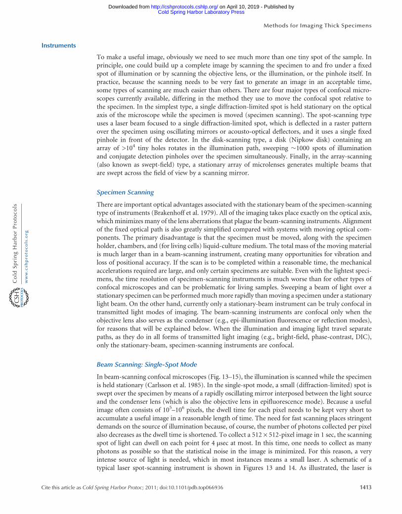
Confocal microscopes can form an image using several different sources of optical information fromthe specimen. A reflectance image can be formed by using the light that is scattered (backscatter) fromthe specimen in the backward direction (i.e., back along the path of the incoming epi-illumination).This light will, of course, have the same wavelength as the original illumination. Colloidal gold labelsare easily visualized in the reflectance mode. The insoluble precipitates formed by the Golgi stain pro-cedure for neurons (Fig. 16) or horseradish peroxidase (HRP) oxidation of substrates such as diami-nobenzidine also give bright backscatter images.

In addition to the straightforward reflectance signal, the confocal microscope can also easily be setup to detect the interference pattern between light reflected from the cell membranes and thatreflected from the underlying substrate (Sato et al. 1990), the technique known as interference reflec-tion contrast microscopy (IRM) (Izzard and Lochner 1976; DePasquale and Izzard 1987, 1991). Thismethod works well with intact living cells (Fig. 17). Fluorescence emitted by the specimen is the mostcommon source of optical information used to generate confocal microscope images. In this case, theimage-forming light has a different wavelength than the illumination, so the fluorescence and reflec-tance signals can be separated using dichromatic beam splitters as in conventional epifluorescencemicroscopes. A particularly valuable feature of the commercial instruments is the ability to acquiresimultaneous, perfectly registered images from multiple different fluorescent labels with (in someinstruments) independent control of the trade-off between sensitivity and resolution in each channel.

As well as forming an image from the emitted fluorescent light that is collected by the objectivelens, most beam-scanning confocals have the ability to simultaneously collect illuminating lightthat passed through the specimen, acquiring a transmitted (e.g., bright-field, phase-contrast, orDIC) image in parallel with the backscatter or epifluorescence image. The quality of these scanned






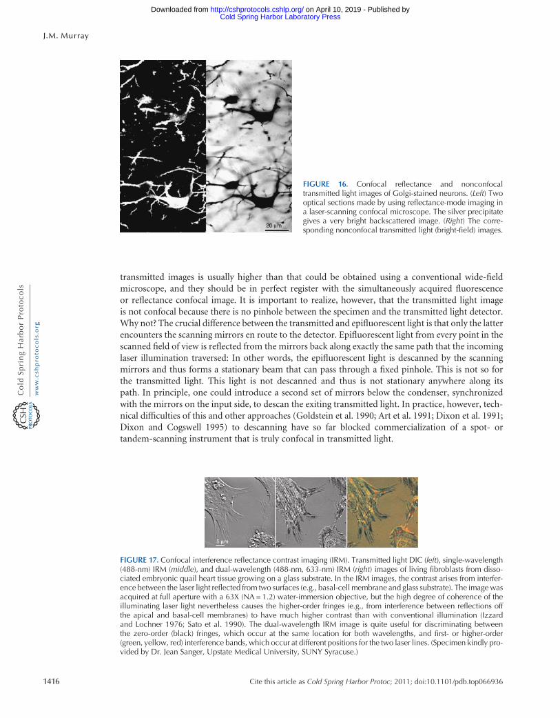
transmitted images is usually higher than that could be obtained using a conventional wide-fieldmicroscope, and they should be in perfect register with the simultaneously acquired fluorescenceor reflectance confocal image. It is important to realize, however, that the transmitted light imageis not confocal because there is no pinhole between the specimen and the transmitted light detector.Why not? The crucial difference between the transmitted and epifluorescent light is that only the latterencounters the scanning mirrors en route to the detector. Epifluorescent light from every point in thescanned field of view is reflected from the mirrors back along exactly the same path that the incominglaser illumination traversed: In other words, the epifluorescent light is descanned by the scanningmirrors and thus forms a stationary beam that can pass through a fixed pinhole. This is not so forthe transmitted light. This light is not descanned and thus is not stationary anywhere along itspath. In principle, one could introduce a second set of mirrors below the condenser, synchronizedwith the mirrors on the input side, to descan the exiting transmitted light. In practice, however, tech-nical difficulties of this and other approaches (Goldstein et al. 1990; Art et al. 1991; Dixon et al. 1991;Dixon and Cogswell 1995) to descanning have so far blocked commercialization of a spot- ortandem-scanning instrument that is truly confocal in transmitted light.

FIGURE 17. Confocal interference reflectance contrast imaging (IRM). Transmitted light DIC (left), single-wavelength(488-nm) IRM (middle), and dual-wavelength (488-nm, 633-nm) IRM (right) images of living fibroblasts from disso-ciated embryonic quail heart tissue growing on a glass substrate. In the IRM images, the contrast arises from interfer-ence between the laser light reflected from two surfaces (e.g., basal-cell membrane and glass substrate). The imagewasacquired at full aperture with a 63X (NA = 1.2) water-immersion objective, but the high degree of coherence of theilluminating laser light nevertheless causes the higher-order fringes (e.g., from interference between reflections offthe apical and basal-cell membranes) to have much higher contrast than with conventional illumination (Izzardand Lochner 1976; Sato et al. 1990). The dual-wavelength IRM image is quite useful for discriminating betweenthe zero-order (black) fringes, which occur at the same location for both wavelengths, and first- or higher-order(green, yellow, red) interference bands, which occur at different positions for the two laser lines. (Specimen kindly pro-vided by Dr. Jean Sanger, Upstate Medical University, SUNY Syracuse.)

FIGURE 16. Confocal reflectance and nonconfocaltransmitted light images of Golgi-stained neurons. (Left) Twooptical sections made by using reflectance-mode imaging ina laser-scanning confocal microscope. The silver precipitategives a very bright backscattered image. (Right) The corre-sponding nonconfocal transmitted light (bright-field) images.


J.M. Murray




Lasers and Fluorescent Labels

The total power required for imaging typical specimens is quite modest (�0.1 mW) when comparedwith the power of commonly available lasers, but the intensity at the focal spot can be enormous(MW/cm2). It is important to use the minimum power necessary to acquire each image, whichusually means reducing the beam intensity by 10- to 100-fold, using neutral density filters or anacousto-optic modulator in the illumination path. At very low laser power, the strength of theemitted fluorescence will increase directly in proportion to increases in the intensity of the illumina-tion. However, as the illumination power is increased, the emitted light will no longer increase in pro-portion because the number of fluorophores already in the excited state becomes a significant fractionof the total fluorophores present. This phenomenon is referred to as ground-state depletion andshould be avoided.

Increases of illumination power beyond the onset of ground-state depletion result in smaller andsmaller increases in emission from the fluorescentmolecules in the focal plane because they aremostlyalready in the excited state. Away from the plane of focus, where the illumination is less intense,increases in laser power will continue to excite more andmore fluorescent molecules. This is an unde-sirable effect because the out-of-focus light does not contribute to the image and the excitedmoleculesare subject to photobleaching. In this respect, multiphoton imaging has a possible advantage over con-focal imaging because the light intensity is not high enough to generatemultiphoton absorption eventsoutside the focal spot. Unfortunately, many fluorophores photobleach faster with multiphoton thanwith single-photon excitation, so the advantage is sometimes not realized in practice (Patterson andPiston 2000).

Each type of laser emits light at a set of characteristic wavelengths, so the type of laser availabledetermines the fluorophores that can be imaged. Table 1 shows the wavelengths available fromsome of the more common lasers and the major peaks in the spectrum from a mercury (Hg) arclamp. It is important to remember that the peaks in the arc lamp spectrum are very much broaderthan the spectral lines from the lasers, and significant emission (5%–10% of peak intensity) occursat all wavelengths between the peaks. Thus the range of fluorophores that can be excited by Hg arcillumination is very much broader than that for any single laser.

Simultaneous Imaging of Multiple Labels

The distribution of wavelengths available from the light source becomes especially important whentwo or more fluorophores must be imaged in the same specimen. In general, one can expect problemswith signal contamination between the two channels (bleed-through) when the emission ranges oftwo fluorophores overlap significantly and one of them is much more strongly excited than theother. For example, a rhodamine class plus a fluorescein class is one popular pair of fluorescentlabels for double-labeling experiments in conventional epifluorescence microscopy, using Hg arc illu-mination at 495 and 546 nm. However, pairs of these fluorophores with spectra similar to rhodamine

TABLE 1. Visible laser and Hg arc emission wavelengths

Source Emission wavelengths (nm)

Ar [351] [364] 458 466 477 488 496 502 514Kr [337] [356] 468 476 482 521 531 568 647ArKr 488 568 647HeNe 543 594 604 612 629 633 1152HeCd 325 442 534 539 636Solid state 355 405 410 440 442 445 457 458 473 488 515 532 555 559 561 628 635

638 639 650 670 685 694 700–1000 tunable 750 780 810Hg arc 313 334 365 405 436 546 577

Unbracketed values are the lines available from the commonly used low-power (5–50 mW), air-cooled lasers. New solid-state lasers are introduced frequently; other wave-lengths will probably be available soon. Many more lines, including those in the UV ranges that are listed in brackets, are available from the large high-power (1–5 W),water-cooled versions of the gas lasers. In contrast to the lasers, the Hg arc lamp emits at all wavelengths between its major peaks, at a level of 5%–10% of the peak intensity.






and fluorescein often give unsatisfactory results in confocal microscopes that use only an argon (Ar) oran argon–krypton (ArKr) laser because these do not emit appropriate wavelengths for efficient exci-tation of the rhodamine-class dye. Some instruments attempt to use the 488- and 514-nm lines of theAr laser to excite the fluorescein class (typical peak excitation at 490 nm) and rhodamine class (exci-tation optimum �550 nm). Only the first fluorophore is efficiently excited at 488 nm, but it has anextended long wavelength tail of emission that completely overlaps the emission spectra of thesecond dye. At 514 nm, both dyes are excited equally (�20% of maximum excitation). This combi-nation of spectral properties and laser excitation wavelengths thus leads to severe problems withbleed-through. The problem is solved by using different fluorophores and/or different lasers. Forexample, the 488-nm Ar plus the 543-nm green helium–neon (HeNe) laser lines work well withthese two dyes, or one can use dye number 1 plus a longer wavelength (Texas Red-class) dye usingthe Ar 488 nm and the 567 lines of the ArKr laser. For (much) more information, spectra, and anexcellent discussion of applications of these and other fluorophores for live cell microscopy, the Mol-ecular Probes catalog, or website (http://www.probes.com/), are invaluable.

As one increases the number of fluorophores used simultaneously, the probability of significantcross talk approaches 100%. There are several approaches to dealing with the problem, and newmethods are introduced regularly. First, one can give up simultaneous data acquisition and insteaduse sequential scans with single laser lines. This works for combinations of fluorophores in whichemission spectra overlap but that can be individually excited by different laser lines. It does notsolve the problem when both emission and excitation spectra overlap extensively. An alternative isto greatly increase the spectral resolution of the detection apparatus (using a dispersive element ofsome kind, be it a prism, grating, or acousto-optic deflector), so that arbitrary wavelength bands ofemission can be collected. Although it is sometimes possible to choose a narrow range of wavelengthsthat gives acceptable discrimination between fluorophores with partially overlapping excitation and/or emission spectra, the detected signal becomes weaker as the detection window is narrowed. One canalso introduce additional criteria for gating the fluorescence output. For instance, fluorophores thathave similar emission and excitation spectra may nevertheless have quite different fluorescent life-times. Very short-pulsed excitation and time-gated detection synchronized to the laser pulses thenallow discrimination based on fluorescent lifetime (Gadella et al. 1993; Cole et al. 2001). Fluorescencepolarization (Massoumian et al. 2003) (or hole-burning plus time-gated polarization-sensitive detec-tion) offers additional possibilities for discrimination.

Inevitably, however, the number of signals that need to be separately detected will increase toexceed the capability of the detection system to discriminate, so ultimately one will have to dealwith the problem of fluorophore cross talk by postacquisition processing. In this approach, multipleimages contaminated with cross talk between different fluorophores are collected, each with a differ-ent combination of excitation and/or emission wavelengths. Reference images are also collected indi-vidually from pure samples of each fluorophore, using the same set of excitation and/or emissioncombinations. The contributions of each fluorophore are then sorted out by, in effect, setting upand solving the appropriate system of simultaneous linear equations for each pixel of the image. Appli-cations of this computational method to karyotyping routinely discriminate between more than 20different colors of fluorescent label (e.g., the spectral karyotype system from Applied SpectralImaging) (Schrock et al. 1996; Ried et al. 1997).

Specimen Preparation

Confocal microscopy is compatible with any of the conventional specimen-preparation methods,including imaging of unprepared living tissue. Images at modest resolution of material down to adepth of �0.2 mm below the surface can be obtained from many tissues if the working distance ofthe objective is large enough. Thicker slices can often be examined completely if they are mountedbetween two thin coverslips and imaged from both sides. For the highest resolution work, sphericalaberration introduced by the sample enforces a much lower limit on specimen thickness. Severeattenuation of both the incoming laser illumination and the exiting fluorescence emission, because


J.M. Murray


http://www.probes.com/

http://www.probes.com/



of scattering by local inhomogeneities of the refractive index of the sample, often limits the quality ofconfocal images deeper than 0.05 mm. Attenuation is sometimes less for multiphoton microscopy,because of the longer wavelength used for illumination, and the fact that a detector pinhole isunnecessary, which gives multiphoton microscopy an advantage over confocal for deep imaging insome tissues. Care is necessary in mounting thick specimens to avoid compressing them while atthe same time minimizing the distance between the coverslip and the specimen. It is also importantto use small coverslips when possible. Large coverslips flex with each motion of the objective lens,causing fluid displacements and specimen motion.

Time-lapse imaging of living samples for extended periods at 37˚C pose several problems. On–offcycling of the sample chamber heater results in vertical movements that shift the plane of focus.Because immersion lenses are usually required, the sample chamber will be strongly thermallycoupled to the objective lens, requiring a separate objective-lens heater, whose cycling also changesthe focal plane. In a typical microscope room, the on–off cycling of the laboratory air conditioner–heater system will cause additional focal shifts. However, with well-designed chambers and lensheaters and a modern laboratory building with good environmental stability, these thermallyinduced shifts are small enough to be barely noticeable under visual observation. Unfortunately,that is not good enough. Even under these ideal conditions, the shifts are still �10-fold larger thanthe vertical resolution of the confocal microscope (Fig. 18). To compensate for these shifts in unat-tended time-lapse imaging, the vertical extent of each 3D stack has to be increased both above andbelow the specimen by the size of the thermal shift. For instance, to be certain of completely capturinga 5-µm thick cell, images might have to be taken over a 15-µm span, tripling the total exposureand making it very difficult to do extended time-lapse imaging. A third problem arises when usingwater-immersion lenses. At 37˚C, the water between the sample chamber and the lens quickly evap-orates, and it is not possible to replace it without interrupting the time-lapse study and movingthe specimen.

After struggling unsuccessfully with these problems, including trials with a wide range of commer-cially available sample chambers and temperature-control systems, we decided to take a different

FIGURE 18. Homemade confocal microscope environmental chamber for live cell imaging. (Left) Front view of thetemperature- and humidity-controlled box that encloses the entire invertedmicroscope except for Hg arc and tungstenlamps. Orange letters indicate the separate pieces of the box: (H) Ultrasonic humidifier (Vicks); (hc) relative-humiditycontroller (RHCN-3A, Omega Engineering); (T) heater–air circulator (Air-Therm, World Precision Instruments).(Middle) The disassembled pieces of the box, which are made of 6-mm acrylic sheet, that fit snugly together andare locked into place with clasps. The front piece (F) has a rectangular aperture through which the eyepieces protrude(orange rectangle). The front and right half of the top (RT) are clear acrylic. The left and right sides (LS, RS), left half of thetop (LT), and back panel (B) are opaque, black acrylic covered with reflective thermal insulating bubble wrap. Theback panel and floor plate remain permanently mounted on the microscope. The remainder of the box disassemblesfor use at room temperature. (Upper right) Top view from the right side, with the top of the box removed. The conden-ser/lamp-housing post of themicroscope tilts backward for access to the stage, pushing a swiveling panel that is set intothe back panel of the box. (Lower right) Graph showing focal-plane shifts with different sample chambers. Blue andgreen lines represent shifts with a commercial sample chamber and objective-lens heater in auto and confocalmodes. The red line represents the shifts with the homemade box. After an initial equilibration period, the focalplane with the homemade box is stable to within �0.2 µm.






approach (Fig. 18). The specifications obtained from the microscope manufacturer revealed the fun-damental problem. According to Zeiss, the overall thermal response for their Axiovert invertedmicro-scope system, including lenses, stage, focus drive, etc., is 10 µm of focal-plane shift for 1˚Ctemperature change. Therefore, to reduce the focal shifts to below the vertical resolution of theconfocal microscope, it would be necessary to stabilize the temperature of the microscope to betterthan 0.04˚C. That is not a realistic goal when the room temperature fluctuates by 1˚C to 2˚C, andthe difference between the room temperature and the sample and/or lens temperature is15˚C–20˚C. Moving the microscope to a warm room held at 37˚C would be one solution, but thehumidity needs to be very high to reduce the evaporation rate of the immersion water. A more user-friendly solution that has worked well for us is to enclose the entire microscope, except for theepi-illumination and transmitted light sources, in a (homemade) box held at 37˚C and 70%–80%humidity (Fig. 18).

Photobleaching and Phototoxicity

In most cases, these two phenomena are actually the same process viewed from two different perspec-tives. When the emphasis is on accurate measurement of the 3D distribution of a fluorophore, thenthe primary concern is with photobleaching. When the emphasis is on observing the fluorophore dis-tribution in a physiologically normal state, then phototoxicity will be the foremost concern. As ageneral rule, for quick observations of living cells at a single time point, photobleaching is the relevantphenomenon, and it is usually a surmountable problem. For repeated observations of the same cell,phototoxicity is the perspective that will be forced on us, because it is always a major problem andusually necessitates accepting compromises that limit image quality.

Modern confocal microscopes can acquire a high-quality digital image with much lower illumina-tion than would be necessary for visual observation of the same sample. For example, Figure 19 showsthe photobleaching of yellow fluorescent protein (YFP) in a living cell observed by confocalmicroscopy. In this specimen, as is often the case, the error because of photobleaching is small fora single image or even a moderately large 3D stack of images. Unfortunately, long before photobleach-ing makes the intensity measurement inaccurate, phototoxicity will have made the experiment irre-levant. To keep the damage to a minimum, careful attention must be paid to optimizing themicroscopy. The goal is to extract the maximum information from the limited number of photonsthat the cell will tolerate before phototoxicity becomes unacceptable.

When the sample is not too thick, the much larger quantum efficiency of CCD cameras comparedwith photomultipliers gives disk-scanning confocals, wide-field, deconvolution, and structured illu-mination methods an important advantage over point-scanning confocal microscopes. For verythick living specimens where photobleaching is a serious problem, multiphoton illumination mayprovide some improvement, although this seems to be dependent on the sample (Patterson andPiston 2000).

Deconvolution of Confocal Images

Can deconvolution methods be applied to confocal images, and is anything gained by doing so? Inprinciple, certainly. Although the confocal pinhole is said to remove out-of-focus light, thisremoval is never perfect, and unquestionably confocal images always show residual effects of theripples in the 3D PSF caused by defocus. An example is shown in Figure 20, a confocal reflectance

FIGURE 19. Loss of fluorescence of YFP because of photobleaching. Fluorescencefrom an YFP-fusion protein expressed in a living cell (a nondiffusible cytoskeletalcomponent) was recorded using 514 nm excitation light in a laser-scanning confo-cal microscope. The illumination intensity, dwell time per pixel, and photomulti-plier gain were adjusted to give an image of acceptable quality using a pinholediameter equivalent to �1 Airy disk. The average fluorescence intensity in asmall regionwas then recorded over the course of repeated scans. The fluorescencedecreased by approximately one-half after 100 scans.


J.M. Murray




image of the same diatom imaged by wide-fieldmicroscopy in Figure 4. Notice that the phase reversalsare seen in the confocal image; the holes change from black to white across the curved diatom surface.This suggests that confocal images might benefit from deconvolving the 3D PSF, and indeed this hasbeen reported (Shaw and Rawlins 1991; Cox and Sheppard 1995; van der Voort and Strasters 1995;Verveer et al. 1999; Boutet de Monvel et al. 2001). However, there are several considerations thatmight make investigators wary of the results, and several more reasons why they might conclude itis not worth the effort.

The first challenge is to determine the correct 3D PSF for a confocal microscope. In theory, thiscan be computed (Wilson and Sheppard 1984), but in practice, the computation is inaccurate, as it isfor conventional wide-field microscopy with high-NA objectives. Can a 3D PSF be experimentallydetermined, as is routinely performed for wide-field microscopes? Unfortunately, the images fromconfocal microscopes often suffer from patterned noise artifacts (Fig. 21). Some of the patternsrepeat with a periodicity that is a significant fraction of the entire field of view, which means thatthey are not represented at their true contrast in the images of tiny beads that are used for PSFmeasurements. Effectively, the PSF varies across the field of view, contrary to the assumptions oftypical deconvolution algorithms. A second concern is the poor SNR of confocal images (Figs. 21–23). This makes it quite difficult to measure the (local) 3D PSF with the accuracy required for reliabledeconvolution and greatly exacerbates the tendency of deconvolution to amplify noise in the raw data.

These concerns apply even to images of thin specimens. If a specimen is thick enough that onereally needs to use a confocal microscope (instead of using wide-field plus deconvolution micro-scopes), then the 3D PSF is certain to be seriously degraded by spherical and chromatic aberration(Figs. 24 and 25), and this distortion will change dramatically between the top and bottom of the3D data stack. In this situation, deconvolution is unlikely to give a correct result.

Finally, it could be reasonably argued that deconvolution comes too late to correct the mostimportant defects of confocal images. The great benefit of deconvolving wide-field images is thatthe SNR is enhanced because at least some of the out-of-focus light can be restored to the in-focusplane, thus increasing its total information content. In a confocal image, however, virtually all ofthe out-of-focus light was thrown away (blocked by the pinhole) before reaching the detector andthus cannot be retrieved by deconvolution. This removes much of the motivation for applying decon-volution methods to confocal images.

Practical Aspects and Tips for Generating Reliable Images

The currently available confocal microscopes are rather delicate, unstable instruments. Theyare typically controlled by complex computer programs and are, therefore, prone to unexplainedcrashes and failed operations or missing functions. For these reasons and more, acquiring high-quality confocal images that faithfully represent the sample is a slow, often frustrating process, andthe path to success is sprinkled with traps for the unwary. Unfortunately, even with a completenovice at the controls, an image of some kind will always appear on the screen. However, distinguish-ing image from garbage takes time and considerable care regardless of how much experience theoperator has.

Below are some guidelines that may help in adjusting the microscope parameters to obtain inter-pretable confocal images. (Additional help can be found in the Troubleshooting Guide.) For the

FIGURE 20. Contrast reversal because of defocus in a confocal image.(Left) A reflectance image of a diatom taken with a confocal microscope(Olympus FluoView 300) using a 60× (NA = 1.4) objective. (Right) Anenlargement of a small portion of the image on the left showing contrastreversals because of changing amounts of defocus. Compare withFigure 4.






FIGURE 22. Spot-scanning confocal images of transgenic Toxoplasma gondii expressing an YFP–α-tubulin fusionprotein. Microtubules near the cell surface are included in these single optical sections. (Left) A typical spot-scanningconfocal image. (Middle) A superior image (Olympus confocal, much less intensity fluctuation); the best ever recordedfrom this specimen. Compare the SNR in this image with the wide-field image in Figure 7. (Right) A graph showing theintensity profile along the red and blue lines in the images.

FIGURE 21. Fluctuations in illumination intensity and polarization in a confocal microscope (Zeiss LSM 510). Mean-corrected images of a uniform specimen (top row) and their power spectra (middle row) acquired with four differentlaser lines. The experiment was performed under conditions that gave >1000 photons per pixel, and thus the expectedsingle-pixel noise in the images is �3%. The images would ideally be of uniform intensity and thus be entirely blackafter subtraction of the mean value but instead show artifactual intensity fluctuations. Deviations from the mean valueof up to ±10% are color coded according to the scale in the top right corner. The power spectra show that each lasercontributes patterned noise with a complex mixture of periodicities. Contrast of the power spectra has been enhancedto make the weaker features visible in the print. Some of the patterns have repeat lengths that are much longer than asingle scan line. (Bottom row) The average fluctuation in intensity in a 100 × 100-pixel image of a uniform, stable flu-orescent sample is plotted for a series of 1000 images acquired at 1-sec intervals (left), or 600 images at 1-min intervals(middle). The expected noise in the average value of 104 pixels is�0.03% (i.e., 0 with 8-bit intensity digitization). Theeffect of these artifacts is to severely degrade the image SNR (see Figs. 22 and 23). The horizontal stripes in the DICimage (bottom row, right) are caused by random changes in plane of polarization that accompany the fluctuationsin intensity of the illumination.


J.M. Murray




preliminary adjustment of imaging parameters, choose an area of the specimen that is roughly equiv-alent to the area that will be recorded but is not the best area. The chosen area will be destroyed duringthe setup phase.

1. Choose the appropriate combination of laser, dichromatic mirror (beam splitter), and emissionfilter (see comments above relevant to imaging multiple fluorophores).

2. Decide what pixel spacing is appropriate for collecting the information you need from this particu-lar sample, and set the magnification or electronic-zoom factor accordingly.

Do not oversample (the pixel spacing should be only slightly smaller than the Nyquist criterion, i.e., slightlyless than one-half of the spatial resolution required for the experiment). Use the highest-NA objective avail-able. For thick samples mounted in aqueous media, a water-immersion objective with a correction collar setto minimize spherical aberration is the best choice (see Interpreting the Results, below). For thinner samples,an oil-immersion lens may work, but the refractive index of the immersion oil must be carefully selected tominimize the spherical aberration for each specimen.

3. Get a ballpark estimate for the imaging parameters.

i. Set the pinhole initially to �1 Airy disk unit.

ii. Set the laser to the minimum power that gives a decent signal at maximum gain on thedetector.

4. Find the linear range of the detector system: Use a pseudocolor lookup table (LUT) that highlightsunderflow (intensity = 0) and overflow (intensity = 255 for 8-bit or 4095 for 12-bit detections) incolor, but is grayscale in between.

i. Scan with the laser off or set to zero power at the scan speed to be used for the specimen, andadjust the offset (dark-current compensator) so that the recorded image intensity is mini-mized but there are no pixels at zero intensity.

FIGURE 24. Confocal optical sections of thick tissue. The developing heart in a chick embryo, labeled with fluorescentantibody against cardiac myosin, was imaged with a 60× (NA = 1.4) oil-immersion objective. (Left) The first opticalsection of a 3D stack of 160 sections spaced at 0.5-µm increments. The first section was�20 µm below the coverslip.(Middle) Section number 30; (right) section number 130. Spherical aberration and scatter increasingly degrade the res-olution, so that the 2.2-µm myofibrillar striations, clearly visible in section number 1, are barely resolved in sectionnumber 130. (Sample kindly provided by Howard Holtzer, University of Pennsylvania.)

FIGURE 23. The number of photons needed to give a maximum signal(gray level = 255) on a typical spot-scanning confocal microscope as afunction of the gain setting (PMT voltage). On this microscope, typicalspecimens require a gain setting of 800–900 V, corresponding to�180–80 photons/pixel at maximum brightness.






ii. Find a region of the specimen that is likely to be the brightest and, with the laser on,decrease the detector gain until the recorded intensity in the brightest region of theimage is safely below the saturation value (e.g., 200 out of the maximum of 255 for an8-bit system).

5. Find the linear range for the specimen: Check that the recorded fluorescence emission increaseslinearly with an increase in laser power up to at least twice the laser power you will use for imaging.

If the emission does not increase in proportion to the laser power (i.e., ground-state depletion is occurring),you will have to sacrifice time resolution (work with lower laser power and longer scan times) or spatialresolution (work with lower laser power and increased pinhole diameter or increased pixel size) or both.

6. Check that you are below the instantaneous damage threshold. With the scan speed and laserpower set at these preliminary values, monitor the image intensity in a selected small area of thespecimen over the course of numerous repeated scans.

One would like to be able to scan dozens of times before the cumulative photobleaching reaches 50%. Ifthe fluorescence is bleaching toomuch, youwill have to sacrifice either temporal resolution (longer intervalsbetween scans in a time-lapse series) or spatial resolution (increased pinhole diameter and spacing betweenoptical sections; increased xy pixel size) or both. If the fluorescence is not bleaching measurably and it is tobe a quick experiment or you are otherwise certain that photodamage is not a concern (lucky you), then youmay decrease the photomultiplier gain (which will decrease the noise) or decrease the pinhole size (whichmay improve contrast and resolution) while increasing the laser power to maintain maximum intensities justbelow saturation.

7. Iteratively readjust the parameters according to Steps 4–6 until the image SNR is optimized.

FIGURE 25. Comparison of laser-scanning confocal microscope and a wide-field microscope performance in imaginga thick tissue (Swedlow et al. 2002). A 5-d-old quail embryo stained with Alexa 488 phalloidin (green) and DAPI (blue)was imaged by laser-scanning confocal (A–C) and wide-field microscopy (D). (A) A low-magnification survey image ofthe entire embryo. The head is at the top of the figure. The arrow points to the developing eye, the region shown athigher magnification in B–E. (B) x–z section (parallel to optical axis) showing position of the coverslip (arrow) andthe location of the focal plane shown in C (dashed line). (C ) A single optical section �50 µm below the exteriorsurface of the embryonic eye. Concentrations of actin at cell cortices are visible. (D) The same embryo imaged bywide-field microscopy and recorded with a CCD camera (Alexa 488 only). The image shown is one of the 60 recordedfrom a series of optical sections. (E) The same optical section as in D after restoration by deconvolution. No cellulardetails are visible in wide-field images of this thick tissue. Scale bars: (A) 1 mm; (C, also for B,D,E) 50 µm. (Images Dand E courtesy of Jason Swedlow, University of Dundee.)


J.M. Murray




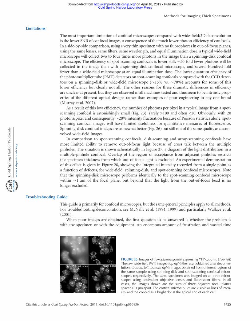
Limitations

The most important limitation of confocal microscopes compared with wide-field/3D deconvolutionis the lower SNR of confocal images, a consequence of the much lower photon efficiency of confocals.In a side-by-side comparison, using a very thin specimen with no fluorophores in out-of-focus planes,using the same lenses, same filters, same wavelength, and equal illumination dose, a typical wide-fieldmicroscope will collect two to four times more photons in the image than a spinning-disk confocalmicroscope. The efficiency of spot-scanning confocals is lower still; �50-fold fewer photons will becollected in the image than with a spinning-disk confocal microscope, and several-hundred-foldfewer than a wide-field microscope at an equal illumination dose. The lower quantum efficiency ofthe photomultiplier tube (PMT) detectors on spot-scanning confocals compared with the CCD detec-tors on a spinning-disk or wide-field microscope (�15% vs. �70%) accounts for some of thislower efficiency but clearly not all. The other reasons for these dramatic differences in efficiencyare unclear at present, but they are observed in all machines tested and thus seem to be intrinsic prop-erties of the different optical designs rather than examples of poor engineering in any one brand(Murray et al. 2007).

As a result of this low efficiency, the number of photons per pixel in a typical image from a spot-scanning confocal is astonishingly small (Fig. 23), rarely >100 and often <20. Obviously, with 20photons/pixel and consequently�20% intensity fluctuation because of Poisson statistics alone, spot-scanning confocal images will have limited usefulness for quantitative measures of fluorescence.Spinning-disk confocal images are somewhat better (Fig. 26) but still not of the same quality as decon-volved wide-field images.

In comparison to spot-scanning confocals, disk-scanning and array-scanning confocals havemore limited ability to remove out-of-focus light because of cross talk between the multiplepinholes. The situation is shown schematically in Figure 27, a diagram of the light distribution in amultiple-pinhole confocal. Overlap of the region of acceptance from adjacent pinholes restrictsthe specimen thickness from which out-of-focus light is excluded. An experimental demonstrationof this effect is given in Figure 28, showing the integrated intensity recorded from a single point asa function of defocus, for wide-field, spinning-disk, and spot-scanning confocal microscopes. Notethat the spinning-disk microscope performs identically to the spot-scanning confocal microscopewithin �1 µm of the focal plane, but beyond that the light from the out-of-focus bead is nolonger excluded.

Troubleshooting Guide

This guide is primarily for confocal microscopes, but the same general principles apply to all methods.For troubleshooting deconvolution, see McNally et al. (1994, 1999) and particularly Wallace et al.(2001).

When poor images are obtained, the first question to be answered is whether the problem iswith the specimen or with the equipment. An enormous amount of frustration and wasted time

FIGURE 26. Images of Toxoplasma gondii expressing YFP-tubulin. (Top left)The rawwide-field (WF) image, (top right) the result obtained after deconvo-lution, (bottom left, bottom right) images obtained from different regions ofthe same sample using spinning-disk and spot-scanning confocal micro-scopes, respectively. The same specimen was imaged on all three micro-scopes using equivalent objective lenses and fluorescent filters. In allcases, the images shown are the sum of three adjacent focal planesspaced 0.3 µm apart. The cortical microtubules are visible as lines of inten-sity and the conoid as a bright dot at the apical end of each cell.






can be avoided if standard samples are available that can be used to compare the system performanceat the moment with its performance in the past (i.e., on a day when good images were obtained).Four simple specimens are useful for this purpose: a resolution test target (e.g., see Fig. 29); an opti-cally flat mirror or bare glass slide; 0.2–0.5-µm diameter beads labeled with multiple fluorophores(e.g., TetraSpeck; Molecular Probes/Invitrogen) that are excited by each of the laser lines and detectedthrough each of the filter sets on the instrument; and a solution of fluorescent dyes covering similarlybroad excitation and emission spectra (e.g., a mixture of 4′,6-diamidino-2-phenylindole (DAPI),Alexa Fluor 488, Alexa Fluor 594, and Alexa Fluor 633 solutions). The beads should be spread intoa film on a coverslip, allowed to dry, and mounted on a thin layer of antifade solution or opticalcement (e.g., Epo-Tek 301; Epoxy Technology). To make the fourth standard specimen, a generouslayer of the solution of fluorescent dyes should be sealed under a coverslip.

On a day when the equipment seems to be in good working order, collect and store a 2D image ofthe resolution test target at optimum focus, a 3D stack of images of the fluorescent beads, and animage of the fluorescent dye solution a few micrometers underneath the coverslip, using the smallestpinhole. Do this for all laser lines and all filter–detector channel combinations. Also collect an X–Z

FIGURE 28. Axial resolution in wide-field (WF) and confocalmicroscopes. Three-dimensional stacks of images of a 0.2-µmdiameter fluorescent bead were collected in a WF,disk-scanning, or spot-scanning confocal microscope. Thegraph shows the total integrated intensity from the bead indifferent focal planes, individually normalized for eachmicroscope. The intensity profile in the WF images afterdeconvolution is also shown. The intensity recorded by thedisk-scanning confocal microscope falls off exactly as withthe spot-scanning microscope for small values of defocusbut then plateaus and remains constant while the spot-scanning intensity continues to decrease to 0.

FIGURE 27. Schematic of the light distribution in a multiple pinhole confocal microscope. (Top left) A vertical slice(i.e., x–z plane) of the distribution of illumination near the focal plane for a single spot of illumination with an objectivelens of NA = 1.2. (Bottom left) The corresponding fluorescence emission with the acceptance angle of the objectivesuperimposed. (Right) The overlap of neighboring illumination cones and acceptance regions, with a spacingbetween adjacent spots/pinholes of d. This limits the region of confocal behavior—that is, the ability to excludelight from out-of-focus planes—to a narrow band on either side of the focal plane. Out-of-focus light that originatesfrom within the confocal region is excluded by the pinholes, but fluorescence coming from more distant planes isaccepted, thus limiting performance in very thick samples.


J.M. Murray




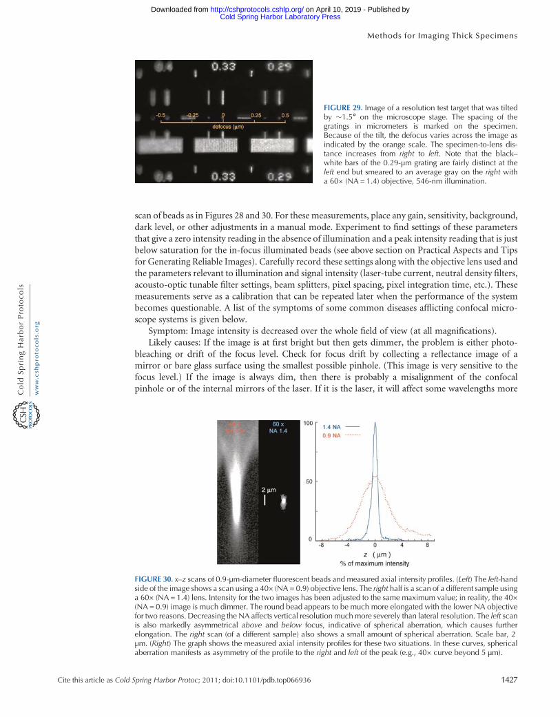
scan of beads as in Figures 28 and 30. For these measurements, place any gain, sensitivity, background,dark level, or other adjustments in a manual mode. Experiment to find settings of these parametersthat give a zero intensity reading in the absence of illumination and a peak intensity reading that is justbelow saturation for the in-focus illuminated beads (see above section on Practical Aspects and Tipsfor Generating Reliable Images). Carefully record these settings along with the objective lens used andthe parameters relevant to illumination and signal intensity (laser-tube current, neutral density filters,acousto-optic tunable filter settings, beam splitters, pixel spacing, pixel integration time, etc.). Thesemeasurements serve as a calibration that can be repeated later when the performance of the systembecomes questionable. A list of the symptoms of some common diseases afflicting confocal micro-scope systems is given below.

Symptom: Image intensity is decreased over the whole field of view (at all magnifications).Likely causes: If the image is at first bright but then gets dimmer, the problem is either photo-

bleaching or drift of the focus level. Check for focus drift by collecting a reflectance image of amirror or bare glass surface using the smallest possible pinhole. (This image is very sensitive to thefocus level.) If the image is always dim, then there is probably a misalignment of the confocalpinhole or of the internal mirrors of the laser. If it is the laser, it will affect some wavelengths more

FIGURE 30. x–z scans of 0.9-µm-diameter fluorescent beads and measured axial intensity profiles. (Left) The left-handside of the image shows a scan using a 40× (NA = 0.9) objective lens. The right half is a scan of a different sample usinga 60× (NA = 1.4) lens. Intensity for the two images has been adjusted to the same maximum value; in reality, the 40×(NA = 0.9) image is much dimmer. The round bead appears to be much more elongated with the lower NA objectivefor two reasons. Decreasing the NA affects vertical resolution muchmore severely than lateral resolution. The left scanis also markedly asymmetrical above and below focus, indicative of spherical aberration, which causes furtherelongation. The right scan (of a different sample) also shows a small amount of spherical aberration. Scale bar, 2µm. (Right) The graph shows the measured axial intensity profiles for these two situations. In these curves, sphericalaberration manifests as asymmetry of the profile to the right and left of the peak (e.g., 40× curve beyond 5 µm).

FIGURE 29. Image of a resolution test target that was tiltedby �1.5˚ on the microscope stage. The spacing of thegratings in micrometers is marked on the specimen.Because of the tilt, the defocus varies across the image asindicated by the orange scale. The specimen-to-lens dis-tance increases from right to left. Note that the black–white bars of the 0.29-µm grating are fairly distinct at theleft end but smeared to an average gray on the right witha 60× (NA = 1.4) objective, 546-nm illumination.






strongly than others. For instance, the Ar/Kr and Kr lasers are very prone to loss of their yellow(568-nm) and red (647-nm) lines while retaining the blue lines (488 or 476 nm).

Symptom: Image intensity is decreased over the periphery of the field of view, which is more pro-nounced at lower magnification.

Likely causes: If the effect is seen in both fluorescence and reflectance images, then it is either amisalignment (most systems) or an intrinsic design problem (older Bio-Rad systems). If the effectis much more pronounced in fluorescent images than in reflectance images, then it indicateschromatic aberration.

Symptom: The resolution is poor.Likely causes: If the problem is apparent both in thin (e.g., fluorescent beads) and thick samples,

then the fault is probably in the alignment of the confocal optics (but first make sure the objective lensis clean). Check that the laser beam is correctly centered on the axis of the objective lens and that theentire back aperture of the lens is filled with incoming light. If the problem is restricted to thicksamples, then spherical aberration is probably the culprit. The newer silicone-immersion and water-immersion objectives with a correction collar greatly ameliorate this problem with thick samples inaqueous media but at the cost of slightly decreased resolution with optically ideal specimens (i.e.,very thin samples with a refractive index the same as glass and positioned immediately adjacent tothe coverslip).

Symptom: Focusing for maximum brightness does not give the sharpest image. The image can bemade bright or sharp but not both.

Likely causes: The system is not confocal. The focal plane for the illumination system does notcoincide with the focal plane for the imaging system. For visible wavelength illumination andimaging, probably the pinhole or an intermediate lens that focuses the light on the pinhole is misa-ligned. If the illumination or imaging wavelengths are ultraviolet (UV) or far red, then a misalignedcollimator lens is the likely culprit.

Symptom: Alternating stripes of higher and lower intensities appear in the image.Likely causes: Mechanical vibration, defects on the scanningmirrors, or an electronic oscillation in

the laser or the detector circuits are the likely causes. To decide between these, collect an image of thefluorescent dye test sample with the largest available pinhole aperture. This image is very insensitive tovibration but still sensitive to electronic oscillations and mirror defects. Mirror defects cause a fixedpattern of bright and dark stripes that does not change between images. Most electronic oscillations(and mechanical vibrations) give a different pattern with each image. Confocal systems from somemanufacturers use single-mode polarization preserving fiber-optic coupling of the laser to the scanhead. Some, but not all, of these systems are very prone to fluctuating illumination intensity andpolarization angle. Painstaking rotational alignment of the fiber polarization axis with the laser polar-ization axis mitigates the effect, but within a few days, the fiber drifts out of alignment and thestripes reappear.

Symptom: A circular bright spot or a set of rings appears at a fixed point in every image.Likely cause: A reflection of the laser beam off an internal glass surface is being detected. If fluor-

escence images are being collected, then an inappropriate set of filters is being used (reflected laserlight is getting through). Most systems now include a quarter-wave plate and polarizer combinationto minimize the problem in reflectance-mode imaging. Probably one of these elements hasbeen rotated.

Symptom: Images from different fluorophores are misregistered.Likely cause: Displacement of a short-wavelength (e.g., DAPI channel) or long-wavelength (e.g.,

CY5 or Alexa 633 channel) from the middle wavelength channels is usually because of misalignmentof a UV–visible or infrared (IR)–visible collimator lens (a component of the illumination path thatcorrects for the small residual chromatic aberration present in all currently available objectivelenses). Be forewarned: Somemanufacturers’ service personnel do not routinely check collimator-lensalignment, so a recent inspection by unsupervised service personnel provides no assurance that thesystem is correctly aligned.


J.M. Murray




STRUCTURED ILLUMINATION METHODS

The goal of these techniques is to improve the images of thick objects by a combination of opticaland computational manipulations. Normally one strives to achieve completely uniform illumination(i.e., completely “unstructured”) across the entire field of view, so that variations in intensity acrossthe image arise solely from variations in the structure of the object. Contrary to what might beexpected, superimposing artifactual intensity fluctuations across the image by using carefully pat-terned nonuniform illumination can actually increase the amount of information about the objectthat is stored in the image.

The development of new techniques for using structured illumination to enhance microscope per-formance is proceeding rapidly and in many directions (Bailey et al. 1993; Neil et al. 1997, 1998, 2000;Wilson et al. 1998; Gustafsson et al. 1999; Hanley et al. 1999, 2000; Gustafsson 2000; Cole et al. 2001;Heintzmann et al. 2001; Dubois et al. 2002). An excellent survey has been written for biologists byHeintzmann and Ficz (2007). As of this writing, most of the techniques have been shown only onvery thin, fixed specimens and are available only in a few specialized laboratories. In this article, wedescribe one method (Neil et al. 1997, 2000) that does work quite well with living specimens of mod-erate thickness and is now commercially available from at least two vendors.

Optical Principles

The basic principle is shown in Figure 29, which illustrates, in a different way, the same informationcontained in Figures 1–3. The figure shows an image of a resolution test target, a series of gratings ofdifferent spacings, which was tilted by�1.5˚ before being photographed. The tilt, which is from rightto left in the image, displaces the sample from the focal plane by an amount that increases, in oppositedirections, away from the center of the field. Notice that the 0.33-µm grating is sharp and well resolvedin the center but becomes quite blurred toward the left. The left side of the 0.29-µm grating is justresolved at a defocus of 0.25 µm, but the right side is completely smeared out when the defocusincreases to 0.5 µm. How can one turn this “problem” into a “solution”?

Imagine the use of a grid of evenly spaced lines as a mask through which the specimen is illumi-nated (Fig. 31). The grid is placed in the light path of the microscope with appropriate lenses to bringits shadow on the specimen into sharp focus in exactly the focal plane of the objective lens. If the speci-men is thin, then the result is an image of the in-focus specimen crossed by a set of sharply demarcatedshadows where the illumination has been interrupted by the mask. If the specimen is thick, thensuperimposed on this in-focus image will be a blurred image of the other planes of the specimen(Figs. 5 and 31). However, the contribution from the out-of-focus planes of the specimen will notbe modulated by the lines of the grating; away from the in-focus plane, the shadow of the gratingquickly becomes smeared and the illumination is uniform, at a level that is the average of the lightand dark bars. Note in Figure 29 that a defocus of 0.5 µm is sufficient to completely eliminate the0.29-µm modulation.

By a simple manipulation, the blurring caused by defocus can be turned into an effective tool for sep-arating in-focus from out-of-focus light when the light is right (i.e., structured). A simple algebraic com-binationof three imagesof theobject illuminatedthroughagratingshiftedbyexactlyone-thirdof itsperiodbetween each image yields an in-focus image uncontaminated by out-of-focus blur (Neil et al. 1997):

Iinfocus = [(I1 − I2)2 + (I1 − I3)2 + (I2 − I3)2]1/2.

The simple sum of the three raw images (I1 + I2 + I3) is of course identical to the normal wide-fieldimage with no grating. The best optical sectioning is obtained when the period of the grating is slightlylarger than the diameter of the Airy disk (Neil et al. 1997).

The grating can be shifted rapidly and precisely (e.g., by a piezoelectric element), and the calcu-lation is very fast. The rate-limiting step for optical sectioning by this method is thus acquiring thethree images. Compared to wide-field plus deconvolution methods, the maximum acquisition rate






would be threefold slower, but the finished product, the in-focus optical sections, is available immedi-ately instead of after 1–2 min as for the deconvolution computation. The total exposure is slightlygreater than for wide-field plus deconvolution methods because the bars of the grating are typicallynot completely opaque. The z-axis resolution is comparable to what is achieved by either confocalor deconvolution methods.

The limitations of this method are not fully known, but it seems that the method has trouble withstructures whose sizes are comparable to the grid spacing. It is expected that the computation wouldalso fail for extremely thick samples, when the background out-of-focus light becomes overwhelming.In that case, the contrast of the grid lines in the raw data will be very low, and the difference between I1,I2, and I3 would become comparable to the noise level. A discussion of some of the technical problemsthat need to be addressed to make the technique useful in practice has been published (Cole et al.2001). The simplicity of the hardware component means that it is cheap to manufacture and canbe user installed as an add-on to virtually any modern microscope. It is safe to predict that thisand other variants of structured illumination microscopy will quickly supplant expensive confocalmicroscopes for many applications on modestly thick specimens, particularly living samples.

INTERPRETING THE RESULTS

The Meaning of Optical Section

Although the images produced by confocal microscopy, deconvolution, and structured illuminationmethods are referred to as optical sections, they differ from true sections in that their top and bottomedges are not sharply defined. In a physical section as cut by a knife in a microtome, there is no ambi-guity about which section contains each point of the original object, at least not at the resolution of theLM. A specified point in the cell was either included in one particular microtome section or it was not,depending on its original position, but there is no intermediate state. An optical section, however,includes some locations fully (i.e., present at their true intensity) and other locations above andbelow at less than their true intensity. There is no sharp cutoff that demarcates what is included inthe optical section and what is excluded. Instead, there is a continuous decrease in the ratio of

FIGURE 31. Structured illumination used for optical sectioning. The light source ismasked by a regular grid,which castsa pattern of stripes on the in-focus object plane. Three images of the thick object are acquired, shifting the grid byone-third repeat between each acquisition. Each image is the sum of contributions from the in-focus plane, which isshadowed by sharply defined stripes, plus blurred out-of-focus planes without distinct stripes. The square root of thesum of the squared difference images removes the out-of-focus blurred light, giving the in-focus plane.


J.M. Murray




image intensity to object intensity for locations further and further away from the midpoint (i.e., theCTF falls off steadily with the distance from the focal plane; Figs. 2 and 3).

A measurement that is commonly used as the analog of section thickness for optical sections is thefull width at half-maximum (FWHM) of the curve that describes the relative intensity of points atdifferent distances from the midpoint of the section. This curve can be measured by collecting aseries of closely spaced optical sections (0.1 µm for the highest-NA lenses) of a small bright object.A small fluorescent bead is a good specimen for this measurement, but any bright object that issmall compared with the expected FWHM can be used. A plot of the total intensity of the image ofthe object in each optical section should give a curve similar to the one in Figure 28, the axial intensityprofile of the 3D PSF for the optical system (equivalent to a vertical line through the center of Fig. 3).For the highest-NA objective lenses, confocal, deconvolved wide-field images, or structured illumina-tion microscopy should give a PSF having an axial FWHMof ≤0.6 µm. Much smaller values of FWHMhave been obtained but not with samples and equipment that are realistic for live cell imaging exper-iments (Bailey et al. 1993; Hell et al. 1997; Gustafsson et al. 1999; Heintzmann and Ficz 2007).

Spherical Aberration

The FWHM of the vertical PSF decreases with the square of the NA of the objective lens. For confocalsystems, the width also decreases with decreasing pinhole size. For all microscopes, the vertical PSF isvery sensitive to the presence of spherical aberration (Figs. 9 and 30). Unfortunately, one is oftenforced to accept a certain amount of spherical aberration when examining living specimens(Fig. 24). The highest-NA oil-immersion objectives are designed for work with a specimen that islocated immediately beneath a coverslip connected to the lens by immersion oil, which obviouslycannot be true for all regions of a thick specimen. Consequently, the image is increasingly degradedby spherical aberration as the focal plane is set deeper and deeper into the specimen. The problem isgreatly ameliorated by using water-immersion objectives. These are water-immersion objectivesdesigned for use with a coverslip, in contrast to older designs (e.g., those used by electrophysiologistsfor patch-clamp studies). They perform better on thick specimens immersed in water than standard(very short working distance) high-NA oil-immersion objectives. However, the PSF of these water-immersion lenses is not yet as good as with the best high-NA oil objectives nor are the water-immersion lenses quite as bright. There are now objectives available designed for use with asilicone-immersion oil of refractive index �1.4 (see Fig. 9) with a correction collar that compensatesfor different depths of imaging.

As illustrated in Figures 9 and 30, spherical aberration leads to an unsymmetrical response todefocus; the image looks different when defocused by the same amount in opposite directionsfrom the in-focus plane. When present, significant spherical aberration is readily visible. A convenientway to check for it is to find a very small, very bright dot of fluorescence and compare its appearance asthe lens is defocused by a small amount (a few micrometers) in either direction. A typical observationis the appearance of bright rings on one side of focus and general fuzziness without rings on the otherside. With the water-immersion lenses, this asymmetry can often be eliminated over an extendedrange of focal planes in a thick specimen by careful adjustment of the correction collar. Withoil-immersion lenses, one can choose an immersion oil with a refractive index that minimizes thespherical aberration at the depth in the specimen where the major interesting features lie (fordepths <�15 µm), but optical performance in other focal planes will be degraded (Fig. 24).

Chromatic Aberration

With modern highly corrected objective lenses and an ideal sample, all wavelengths of light in thevisible range should be focused to the same point at an accuracy of better than 0.1 µm (Keller1995). However, if the mixture of refractive indices in the sample deviates from the design parametersof the objective lens sufficiently to cause noticeable spherical aberration, then chromatic aberration isalso likely to be induced. The lens design is specific not only for a particular arrangement of refractiveindices but also for the way in which those refractive indices vary with wavelength (dispersion). It is






unlikely that the specimen dispersion matches the design specifications, resulting in a shift in focalposition according to wavelength. Figure 32 shows this behavior in a series of optical sections of asingle bead. In this case, the chromatic aberration is caused not by the sample but by misalignmentof collimator lenses that are supposed to correct the confocal system for residual chromatic aberrationin the objective, allowing it to be used with UV and IR as well as visible light.

As the composite image at the top of Figure 32 shows, chromatic aberration is a serious problem indetermining colocalization of different fluorescent molecules. In an extended sample, complicatedartifactual shifts are observed because the direction and amount of apparent shift between differentcolors varies with position in the field of view. Interpretation of slight differences in localizationdemands careful control experiments to rule out chromatic aberration.

Chromatic aberration is of particular concern with confocal microscopes (Hell and Stelzer 1995;Keller 1995). If the focal spot for the illumination wavelength is not in the same position as the focalspot seen through the pinhole aperture, then the system is not confocal. In this situation, image inten-sity is severely decreased.

SNR

Live cell imaging is considerably more demanding than observation of fixed samples. The motivationto invest the extra time and effort is often the need to observe changes in distribution or amount ofsome fluorescent molecule. To be confident, however, that an observed change is real, rather than duesimply to random fluctuations in the image intensity, the investigator must consider the SNR in theimage. Some simple calculations are involved, but math phobes should not be discouraged. Thissimple calculation can prevent a lot of wasted time.

Suppose that an experiment requires detecting changes of 25% or more in the local concentrationof a fluorescent molecule. As an example, consider the cells shown in Figure 7. The objective of theexperiment will be to follow the incorporation and removal of YFP tubulin at the growing and shrink-ing ends of microtubules. Because this specimen is thin enough that the background fromout-of-focus light is not overwhelming, it is appropriate to image it using any of the microscopic tech-niques described in this article.

To restate the experimental requirement, the SNR in the image must be large enough to be con-fident that a 25% increase or decrease in fluorescence at the end of a microtubule is not just because ofrandom noise. To draw this conclusion with 95% confidence, the expected fractional change in signal(i.e., 0.25S) must be greater than twice the standard deviation (i.e., greater than twice the noise, 2N).Thus, SNR must be at least 8 for this measurement to succeed. Expressing the required precision as a

FIGURE 32. Chromatic aberration in confocal images. Eleven optical sections, spaced at 0.2-µm intervals, of a single,0.2-µm diameter bead labeled with four different fluorophores. The dotted cross in each sectionmarks the x–y locationof the center of the bead in the green image at best focus. Notice that the other three wavelength bands are shifted in x,y, and z with respect to the green. The yellow and blue images also reveal some spherical aberration. A compositecolor image for the sixth optical section is shown at the top. (Red) Excitation (ex), 633 nm; emission (em), >650nm. (Yellow) ex, 568 nm; em, 585–615 nm. (Green) ex, 488 nm; em, 505 nm–600 nm. (Blue) ex, 364 nm; em,385–470 nm with a 63× (NA = 1.2), water-immersion lens.


J.M. Murray




fractional change P (i.e., 25% precision in the measurement of Smeans P = 0.25), then for 95% con-fidence, SNR must be >2/P.

To decide if this experiment is feasible, a rough estimate of the signal and its standard deviation isneeded. First, locate an area of a typical sample that is similar to the region of interest. Second, collecttwo images in rapid succession from this area without changing anything between exposures (avoidphotobleaching). In the absence of noise, these two images should be identical. Thus, the differencebetween them can be used to estimate the noise level in a typical measurement. In fact, the standarddeviation of this difference image, call it s, is

��2

√times the standard deviation of a single pixel in the

original images. The noise in the measurement of microtubule fluorescence will be larger than sbecause the background will have to be subtracted. If the ratio of background to total intensity is b,then the standard deviation in one pixel of the background-corrected microtubule fluorescenceimage will be a factor

��1+ b

√larger than the standard deviation in the raw-intensity measurement.

In Figure 7, b = 0.95 before deconvolution and 0.8 after deconvolution. Finally, note that the targetarea for the measurement is more than a single pixel. If the target includes n pixels and the averagefluorescence per pixel of microtubule after background correction is denoted by F, then

SNR ;F

s��(1+ b)/2n√

For the experiment in Figure 7, F was �50 (out of 4095 maximum for the 12-bit CCD), averagedover a 5 × 5-pixel box, s was �12, and b was 0.95, giving an SNR = 21. Thus, the images collectedunder these conditions are indeed good enough to detect the hoped-for change in YFP-tubulinincorporation.

Now suppose one contemplated doing this experiment with a spot-scanning confocal microscopeinstead of wide-field plus deconvolution microscopes. Doing this simple calculation beforehandwould save a lot of time and frustration because one would probably find that the experimentcannot be performed with a spot-scanning confocal microscope. Typical numbers (Zeiss LSM510)would be roughly F� 20 (out of 255 maximum for 8-bit detection), s� 30, b = 0.5, which for thesame size target gives a SNR = 4 (compare Fig. 7 and Fig. 22).

Point-scanning confocal microscope images are much noisier than wide-field images for severalreasons. In a side-by-side comparison, using a very thin specimen with no fluorophores inout-of-focus planes, using the same lenses, same filters, same wavelength, and equal illuminationdoses, a typical wide-field microscope will collect two to four times more photons in the imagethan a spinning-disk confocal microscope. The efficiency of spot-scanning confocals is lower still;�50-fold fewer photons collected in the image than with a spinning-disk confocal microscope andseveral-hundred-fold fewer than a wide-field microscope, at an equal illumination dose. The lowerquantum efficiency of the PMT detectors on spot-scanning confocals compared with the CCD detec-tors on spinning-disk or wide-field microscopes (�15% vs. �70%) accounts for some of this lowerefficiency but clearly not all.

The other reasons for these dramatic differences in efficiency are unclear at present, but they areobserved in all machines tested and thus seem to be intrinsic properties of the different optical designsrather than examples of poor engineering in any one brand (Murray et al. 2007). In addition to havinglower signals, many confocal microscopes add a large amount of unnecessary noise to the image, gen-erated by electronic artifacts in the detector circuitry (Fig. 21) and random fluctuations in the laserillumination intensity. Figure 33 shows a direct comparison of the noise in the illumination of alaser-scanning confocal microscope and a wide-field microscope. It should be emphasized that thisextra noise in the confocal microscope is entirely unnecessary, simply a matter of poor design inmost of the commercially available instruments.

Disk-scanning confocals, which use CCD detectors, have much better SNR than point-scanninginstruments for the same exposure levels. The noise level in images from the structured illuminationmethod described above will be increased by the processing steps needed to calculate the in-focus






image, butmodel calculations suggest that this effect will be less than a factor of 2. Thus, the structuredillumination technique also has the potential for giving an image SNR substantially higher than thecommercially available point-scanning confocals.

Why Confocal?

After this comparison of SNR with a thin sample, it is perhaps worth restating the message of theintroduction to this article: Each of the microscopic techniques described here has its own realmwithin which it reigns unchallenged and outside of which it must take second place to otherapproaches. When specimen thickness is modest, the SNR of the raw data acquired with a wide-fieldmicroscope is high enough to allow excellent contrast enhancement by restoration methods suchas deconvolution or structured illumination. As the thickness and background fluorescence increases,wide field and/or deconvolution eventually fail, and the best images will be acquired with a spinning-disk or array-scanning confocal microscope. Finally, when the sample is very thick, onlypoint-scanning confocal or multiphoton techniques are useful. As a counterpoint to the thin-sampleSNR comparison, Figure 25 shows a comparison between point-scanning confocal microscopes andwide-field plus deconvolution microscopes with a sample that is definitely in the confocal realm.

When a new specimen is to be imaged, it is convenient to have a rule of thumb for deciding whichmethod of microscopy is likely to give the best results. The magnitude of a simple specimen-dependent parameter that we have called the haziness index (H) (Murray et al. 2007) provides anumerical criterion for choosing the most appropriate mode of microscopy. H is computed as aratio of background to signal in a wide-field image: the intensity of background from out-of-focusfluorescence divided by the intensity of the fluorescence from a small in-focus object. Small heremeans comparable in size to the Airy disk. For specimens with very large background, the intensityof such small objects will be unmeasurable in a wide-field microscope, so it is necessary to estimateH by some indirect means. Often it will be possible to find a thin edge of the specimen where the back-ground is not overwhelming andmeasurement of the intensity of some small object of interest is poss-ible in a wide-field microscope. This number could then be combined with a wide-field measurementof the background in the thickest region of the specimen to give a good estimate of H. Alternatively, ifboth signal and background could be measured in a thin specimen, then knowing its thickness relativeto a thicker specimen would be sufficient to calculate the value of H in the regions that are too thick forwide-field microscopy.

FIGURE 33. Fluctuations in illumination intensity in a confocal versus wide-field microscope. (Top) The average inten-sity in a 100 × 100-pixel image of a uniform, stable, fluorescent sample is plotted for a series of 1000 images acquiredat 1-sec intervals, for a point-scanning confocal microscope and a wide-field microscope with a CCD detector.(Bottom) The intensity from a single pixel in a sequence of 100 successive images of the same specimen is plotted.


J.M. Murray




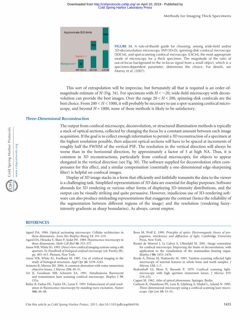
This sort of extrapolation will be imprecise, but fortunately all that is required is an order-of-magnitude estimate of H (Fig. 34). For specimens with H <�20, wide-field microscopy with decon-volution can provide the best images. Over the range 20 <H < 200, spinning-disk confocals are thebest choice. From 200 <H < 1000, it will probably be necessary to use a spot-scanning confocal micro-scope, and beyond H = 1000, none of these methods is likely to be satisfactory.

Three-Dimensional Reconstruction

The output from confocal microscopy, deconvolution, or structured illumination methods is typicallya stack of optical sections, collected by changing the focus by a constant amount between each imageacquisition. If the goal is to collect enough information to permit a 3D reconstruction of a specimen atthe highest resolution possible, then adjacent optical sections will have to be spaced at increments ofroughly half the FWHM of the vertical PSF. The resolution in the vertical direction will always beworse than in the horizontal direction, by approximately a factor of 3 at high NA. Thus, it iscommon in 3D reconstructions, particularly from confocal microscopes, for objects to appearelongated in the vertical direction (see Fig. 30). The software supplied for deconvolution often com-pensates for this effect, and a similar compensation (essentially a one-dimensional edge-sharpeningfilter) is helpful on confocal images.

Display of 3D image stacks in a form that efficiently and faithfully transmits the data to the vieweris a challenging task. Simplified representations of 3D data are essential for display purposes. Softwareabounds for 3D rendering or various other forms of displaying 3D-intensity distributions, and theoutput can be visually striking and quite persuasive. However, injudicious use of 3D-rendering soft-ware can also produce misleading representations that exaggerate the contrast (hence the reliability ofthe segmentation between different regions of the image) and the resolution (rendering fuzzy-intensity gradients as sharp boundaries). As always, caveat emptor.

REFERENCES

Agard DA. 1984. Optical sectioning microscopy: Cellular architecture inthree dimensions. Annu Rev Biophys Bioeng 13: 191–219.

Agard DA, Hiraoka Y, Shaw P, Sedat JW. 1989. Fluorescence microscopy inthree dimensions. Meth Cell Biol 30: 353–377.

AmosWB,White JG. 1995. Direct view confocal imaging systems using a slitaperture. In Handbook of biological confocal microscopy (ed. Pawley JB),pp. 403–415. Plenum, New York.

Amos WB, White JG, Fordham M. 1987. Use of confocal imaging in thestudy of biological structures. Appl Opt 26: 3239–3243.

Arimoto R, Murray JM. 2004. A common aberration with water-immersionobjective lenses. J Microsc 216: 49–51.

Art JJ, Goodman MB, Schwartz EA. 1991. Simultaneous fluorescentand transmission laser scanning confocal microscopy. Biophys J 59:155a.

Bailey B, Farkas DL, Taylor DL, Lanni F. 1993. Enhancement of axial resol-ution in fluorescence microscopy by standing-wave excitation. Nature366: 44–48.

Born M, Wolf E. 1999. Principles of optics: Electromagnetic theory of pro-pagation, interference and diffraction of light. Cambridge UniversityPress, New York.

Boutet de Monvel J, Le Calvez S, Ulfendahl M. 2001. Image restorationfor confocal microscopy: Improving the limits of deconvolution, withapplication to the visualization of the mammalian hearing organ.Biophys J 80: 2455–2470.

Boyde A, Petran M, Hadravsky M. 1983. Tandem scanning reflected lightmicroscopy of internal features in whole bone and tooth samples. JMicrosc 132: 1–7.

Brakenhoff GJ, Blom P, Barends P. 1979. Confocal scanning light-microscopy with high aperture immersion lenses. J Microsc 117:219–232.

Cagnet M. 1962. Atlas of optical phenomena. Springer, Berlin.Carlsson K, Danielsson PE, Lenz R, Liljeborg A, Majlof L, Aslund N. 1985.

Three-dimensional microscopy using a confocal scanning laser micro-scope. Opt Lett 10: 53–55.

FIGURE 34. A rule-of-thumb guide for choosing, among wide-field and/or3D-deconvolution microscopy (WF/3D-D), spinning-disk confocal microscopy(SDCM), and spot-scanning confocal microscopy (LSCM), the most appropriatemode of microscopy for a thick specimen. The magnitude of the ratio ofout-of-focus background to the in-focus signal from a small object, which is aspecimen-dependent parameter, determines the choice. For details, seeMurray et al. (2007).






Carrington WA, Lynch RM, Moore ED, Isenberg G, Fogarty KE, Fay FS.1995. Superresolution three-dimensional images of fluorescence incells with minimal light exposure. Science 268: 1483–1487.

Castleman KR. 1979. Digital image processing Prentice Hall, EnglewoodCliffs, NJ.

Castleman KR. 1996. Digital image processing, 2nd ed. Prentice Hall, Engle-wood Cliffs, NJ.

Cole MJ, Siegel J, Webb SE, Jones R, Dowling K, Dayel MJ, Parsons-Karavassilis D, French PM, Lever MJ, Sucharov LO, et al. 2001.Time-domain whole-field fluorescence lifetime imaging with opticalsectioning. J Microsc 203: 246–257.

Cox G, Sheppard CJR. 1995. Effects of image deconvolution on optical sec-tioning in conventional and confocal microscopes. Biol Imag 1: 82–95.

DePasquale JA, Izzard CS. 1987. Evidence for an actin-containing cyto-plasmic precursor of the focal contact and the timing of incorporationof vinculin at the focal contact. J Cell Biol 105: 2803–2809.

DePasquale JA, Izzard CS. 1991. Accumulation of talin in nodes at the edgeof the lamellipodium and separate incorporation into adhesion plaquesat focal contacts in fibroblasts. J Cell Biol 113: 1351–1359.

Dixon AE, Cogswell C. 1995. Confocal microscopy with transmitted light. InHandbook of biological confocal microscopy (ed. Pawley JB), pp. 479–490.Plenum, New York.

Dixon AE, Damaskinos S, Atkinson MR. 1991. A scanning confocalmicroscope for transmission and reflection imaging. Nature 351:551–553.

Dubois A, Vabre L, Boccara AC, Beaurepaire E. 2002. High-resolution full-field optical coherence tomography with a Linnik microscope. Appl Opt41: 805–812.

Egger MD, Petran M. 1967. New reflected light microscope for viewingunstained brain and ganglion cells. Science 157: 305–307.

Egger MD, Gezari W, Davidovits P, Hadravsky M, Petran M. 1969.Observation of nerve fibers in incident light. Experientia 25: 1225–1226.

Erhardt A, Zinser G, Komitowski D, Bille J. 1985. Reconstructing 3-D light-microscopic images by digital image processing. Appl Opt 24: 194–200.

Fay FS, Carrington W, Fogarty KE. 1989. Three-dimensional moleculardistribution in single cells analysed using the digital imaging micro-scope. J Microsc 153: 133–149.

Femino AM, Fay FS, Fogarty K, Singer RH. 1998. Visualization of singleRNA transcripts in situ. Science 280: 585–590.

Gadella T, Jovin TM, Clegg RM. 1993. Fluorescence lifetime imagingmicroscopy (FLIM): Spatial resolution of microstructures on the nano-second time scale. Biophys Chem 48: 221–239.

Goldstein SR, Hubin T, Rosenthal S, Washburn C. 1990. A confocal video-rate laser-beam scanning reflected-light microscope with no movingparts. J Microsc 157: 29–38.

Gustafsson MG. 2000. Surpassing the lateral resolution limit by a factorof two using structured illumination microscopy. J Microsc 198: 82–87.

Gustafsson MG, Agard DA, Sedat JW. 1999. I5M: 3D widefield lightmicroscopy with better than 100 nm axial resolution. J Microsc 195:10–16.

Hanley QS, Verveer PJ, Gemkow MJ, Arndt-Jovin D, Jovin TM. 1999. Anoptical sectioning programmable array microscope implemented witha digital micromirror device. J Microsc 196: 317–331.

Hanley QS, Verveer PJ, Arndt-Jovin DJ, Jovin TM. 2000. Three-dimensionalspectral imaging by Hadamard transform spectroscopy in a program-mable array microscope. J Microsc 197: 5–14.

Heintzmann R, Ficz G. 2007. Breaking the resolution limit in lightmicroscopy. Methods Cell Biol 81: 561–580.

Heintzmann R, Hanley QS, Arndt-Jovin D, Jovin TM. 2001. A dual pathprogrammable array microscope (PAM): Simultaneous acquisition ofconjugate and non-conjugate images. J Microsc 204: 119–135.

Hell SW, Stelzer EH. 1995. Lens aberrations in confocal fluorescencemicroscopy. In Handbook of biological confocal microscopy (ed.Pawley J), pp. 347–354. Plenum, New York.

Hell SW, Schrader M, van der Voort HT. 1997. Far-field fluorescencemicroscopy with three-dimensional resolution in the 100-nm range.J Microsc 187: 1–7.

Hiraoka Y, Sedat JW, Agard DA. 1990. Determination of three-dimensionalimaging properties of a light microscope system. Partial confocal behav-ior in epifluorescence microscopy. Biophys J 57: 325–333.

Holmes TJ. 1992. Blind deconvolution of quantum-limited incoherentimagery:Maximum-likelihood approach. J Opt Soc AmA 9: 1052–1061.

Hopkins HH. 1955. The frequency response of a defocused optical system.Proc R Soc London, Ser A 231: 91–103.

Izzard CS, Lochner LR. 1976. Cell-to-substrate contacts in living fibroblasts:An interference reflexion study with an evaluation of the technique.J Cell Sci 21: 129–159.

Juskaitis R, Wilson T, Neil MA, Kozubek M. 1996. Efficient real-time con-focal microscopy with white light sources. Nature 383: 804–806.

Kam Z, Hanser B, Gustafsson MG., Agard DA, Sedat JW. 2001. Compu-tational adaptive optics for live three-dimensional biological imaging.Proc Natl Acad Sci 98: 3790–3795.

Keller HE. 1995. Objective lenses for confocal microscopy. In Handbook ofbiological confocal microscopy (ed JB Pawley), pp. 111–126. Plenum,New York.

Lichtman JW, Sunderland WJ, Wilkinson RS. 1989. High-resolution imagingof synaptic structure with a simple confocal microscope. New Biol 1:75–82.

Markham J, Conchello JA. 2001. Artefacts in restored images due tointensity loss in three-dimensional fluorescence microscopy. J Microsc204: 93–98.

Massoumian F, Juskaitis R, Neil MA,Wilson T. 2003. Quantitative polarizedlight microscopy. J Microsc 209: 13–22.

McNally JG, Preza C, Conchello JA, Thomas LJ. 1994. Artifacts incomputational optical-sectioning microscopy. J Opt Soc Am A 11:1056–1067.

McNally JG, Karpova T, Cooper J, Conchello JA. 1999. Three-dimensionalimaging by deconvolution microscopy. Methods 19: 373–385.

Minsky M. 1961. “Microscopy apparatus.” U.S. Patent 3013467.Minsky M. 1988. Memoir on inventing the confocal scanning microscope.

Scanning 10: 128–138.Murray JM, Appleton PL, Swedlow JR, Waters JC. 2007. Evaluating per-

formance in three-dimensional fluorescence microscopy. J Microsc228: 390–405.

NeilMA, Juskaitis R,Wilson T. 1997.Method of obtaining optical sectioningby using structured light in a conventional microscope. Opt Lett 22:1905–1907.

Neil MA, Juskaitis R, Wilson T. 1998. Real time 3D fluorescence microscopyby two beam interference illumination. Opt Commun 153: 1–4.

Neil MA, Squire A, Juskaitis R, Bastiaens PI, Wilson T. 2000. Wide-fieldoptically sectioning fluorescence microscopy with laser illumination.J Microsc 197: 1–4.

Patterson GH, Piston DW. 2000. Photobleaching in two-photon excitationmicroscopy. Biophys J 78: 2159–2162.

Petran M, Hadravsky M, Egger MD, Galambos R. 1968. Tandem scanningreflected light microscope. J Opt Soc Am A 58: 661–664.

Petran M, Hadravsky M, Benes J, Boyde A. 1986. In vivo microscopyusing the tandem scanning microscope. Ann N Y Acad Sci 483:440–447.

Ried T, Koehler M, Padilla-Nash H, Schrock E. 1997. Chromosome analysisby spectral karyotyping. In Cells: A laboratory manual, Vol. 3 (ed.Spector DL et al.), pp. 113-1–113-9. Cold Spring Harbor LaboratoryPress, Cold Spring Harbor, NY.

Sato M, SardanaMK, Grasser WA, Garsky VM,Murray JM, Gould RJ. 1990.Echistatin is a potent inhibitor of bone resorption in culture. J Cell Biol111: 1713–1723.

Scalettar BA, Swedlow JR, Sedat JW, Agard DA. 1996. Dispersion, aberrationand deconvolution in multi-wavelength fluorescence images. J Microsc182: 50–60.

Schrock E, duManoir S, Veldman T, Schoell B, Wienberg J, Ferguson-SmithMA, Ning Y, Ledbetter DH, Bar-Am I, Soenksen D, et al. 1996. Multi-color spectral karyotyping of human chromosomes. Science 273:494–497.

Shao ZF, Baumann O, Somlyo AP. 1991. Axial resolution of confocalmicroscopes with parallel-beam detection. J Microsc 164: 13–19.

Shaw PJ, Rawlins DJ. 1991. The point-spread function of a confocalmicroscope—Its measurement and use in deconvolution of 3-D data.J Microsc 163: 151–165.

Stokseth PA. 1969. Properties of a defocused optical system. J Opt Soc Am59: 1314–1321.

Swedlow JR, Hu K, Andrews PD, Roos DS, Murray JM. 2002. Measuringtubulin content in Toxoplasma gondii: A comparison of laser-scanningconfocal and wide-field fluorescence microscopy. Proc Natl Acad Sci 99:2014–2019.


J.M. Murray




van der Voort HTM, Strasters KC. 1995. Restoration of confocal images forquantitative image analysis. J Microsc 178: 165–181.

Verveer PJ, Gemkow MJ, Jovin TM. 1999. A comparison of image restor-ation approaches applied to three-dimensional confocal and wide-fieldfluorescence microscopy. J Microsc 193: 50–61.

Wallace W, Schaefer LH, Swedlow JR. 2001. A workingperson’s guideto deconvolution in light microscopy. BioTechniques 31: 1076–1082.

Watson TF, Juskaitis R, Wilson T. 2002. New imaging modes for lenslet-array tandem scanning microscopes. J Microsc 205: 209–212.

Wilson T, Sheppard CJR. 1984. Theory and practice of scanning opticalmicroscopy. Academic, London.

Wilson T, Neil MA, Juskaitis R. 1998. Real-time three-dimensional imagingof macroscopic structures. J Microsc 191: 116–118.

Xiao GO, Kino GS. 1987. A real-time scanning optical microscope. SPIEScan Imag Tech 809: 107–113.






doi: 10.1101/pdb.top066936Cold Spring Harb Protoc; John M. Murray and Structured IlluminationMethods for Imaging Thick Specimens: Confocal Microscopy, Deconvolution,

ServiceEmail Alerting click here.Receive free email alerts when new articles cite this article -

CategoriesSubject Cold Spring Harbor Protocols.Browse articles on similar topics from

(12 articles)Photobleaching (100 articles)Multi-Photon Microscopy

(574 articles)Imaging/Microscopy, general (116 articles)Image Analysis

(506 articles)Fluorescence (109 articles)Confocal Microscopy

(514 articles)Cell Imaging (1318 articles)Cell Biology, general

http://cshprotocols.cshlp.org/subscriptions go to: Cold Spring Harbor Protocols To subscribe to

© 2011 Cold Spring Harbor Laboratory Press


http://cshprotocols.cshlp.org/cgi/alerts/ctalert?alertType=citedby&addAlert=cited_by&saveAlert=no&cited_by_criteria_resid=protocols;10.1101/pdb.top066936&return_type=article&return_url=http://cshprotocols.cshlp.org/content/10.1101/pdb.top066936.full.pdf

http://cshprotocols.cshlp.org/cgi/collection/cell_biology_general

http://cshprotocols.cshlp.org/cgi/collection/cell_imaging

http://cshprotocols.cshlp.org/cgi/collection/confocal_microscopy

http://cshprotocols.cshlp.org/cgi/collection/fluorescence

http://cshprotocols.cshlp.org/cgi/collection/image_analysis

http://cshprotocols.cshlp.org/cgi/collection/imaging_microscopy_general

http://cshprotocols.cshlp.org/cgi/collection/multi-photon_microscopy

http://cshprotocols.cshlp.org/cgi/collection/photobleaching

http://cshprotocols.cshlp.org/cgi/subscriptions



methods for imaging thick specimens: confocal microscopy, deconvolution, and structured

Documents