comparison of wideﬁeld/deconvolution and confocal ... · dimensional (3d) image, or to exclude...

INTRODUCTION

The biggest limitation inherent in optical microscopy is its lateralspatial resolution, which is determined by the wavelength of thelight used and the numerical aperture (NA) of the objective lens.Another important limitation is the resolution in the direction ofthe optical axis, conventionally called z, which is related to thedepth of field. The presence of a finite aperture gives rise to unde-sirable and rather complicated characteristics in the image. Inessence, the depth of field depends on the size of structure orspatial frequency being imaged. Fine image detail, which is gen-erally of most interest, has a small depth of field, and only featureswithin a small distance of the focal plane contribute to the image.On the other hand, large structures — low spatial frequency com-ponents — have a relatively large depth of field, and contribute tothe detected image seen at distant focal planes. This is very notice-able in dark-field imaging modes, such as epi-fluorescence, andmeans that the fine image detail may be swamped by low resolu-tion “out-of-focus” light and thus either lost, or visualized withvery much reduced contrast.

The principle advantage of confocal microscopy for biologi-cal imaging is that the optical arrangement has the effect of elim-inating much of the out-of-focus light from detection, thereforeimproving the fidelity of focal sectioning (and hence the three-dimensional imaging properties), and increasing the contrast of the fine image detail. But the rejection of the out-of-focus lightnecessarily means that a proportion of the light emitted by thespecimen is intentionally excluded from measurement. All illumi-nation of the specimen has deleterious effects — bleaching of thefluorochrome or phototoxicity to living cells. These specimen-dependent factors are the ultimate limitation to the quality of theimage, and inevitably confocal imaging does not detect much ofthe emitted light.

An alternative way of removing the out-of-focus light involvesrecording images at a series of focal planes using a conventionalmicroscope, often called widefield (WF) to distinguish it from confocal imaging, and then using a detailed knowledge of theimaging process to correct for it by computer image processing.This procedure is called deconvolution, and its application to bio-logical problems actually preceded the widespread introduction ofbiological confocal microscopes (Castleman, 1979; Agard andSedat, 1983; Agard et al., 1989). In contrast to confocal imaging,up to 30% of the total fluorescent light emitted by the specimencan be recorded (i.e., all the light that can be collected by a single,high-NA objective). This chapter examines the question: Is it better to record all the light emitted and process the WF images to

redistribute the out-of-focus light to produce a more accurate three-dimensional (3D) image, or to exclude the out-of-focus light frommeasurement in the first place by confocal optics and then decon-volve the confocal data?

THE POINT SPREAD FUNCTION: IMAGING ASA CONVOLUTION

In order to derive a soundly based description of the degradationintroduced by an optical microscope, especially if any attempt isto be made to reverse this degradation, it is necessary to be ableto describe the relation between the specimen and its optical imagein mathematical terms. We shall give here a very condensed expla-nation — the interested reader is referred elsewhere for more rig-orous mathematical derivations (Agard et al., 1989; Shaw, 1993;Young, 1989; and Chapters 20, 21, 22, 24, and 25, this volume).Within some quite general limitations, the object (specimen) andimage are related by an operation known as convolution. In a con-volution, each point of the object is replaced by a blurred imageof the point having a relative brightness proportional to that of theobject point. The final image is the sum of all these blurred pointimages. The way each individual point is blurred is described bythe point spread function (PSF), which is simply the image of asingle point. This is illustrated diagrammatically in Figure 23.1.

The conditions that must be met for an imaging process to bedescribed as a convolution are that it should be linear and shiftinvariant (Young, 1989). Imagine cutting the specimen into twoparts and imaging each part separately with the microscope. Ifadding these two subimages together produces the same result asimaging the whole specimen, and does this irrespective of how thespecimen is cut up, then the imaging is said to be linear. If theimaging is indeed linear, then the specimen can be imagined cutup into smaller and smaller pieces, until the size of each piece iswell below the resolution limit, and can be considered to be simplya point. The image is then the sum of the images of each of thepoints, each multiplied by a function corresponding to the amountof light coming from that point. The multiplication and summingis represented mathematically by an operation called convolution.Shift invariance simply means that the imaging characteristics andthus the PSF are the same over the whole field of view, andknowing one PSF is enough to characterize the imaging propertiesof the microscope. (Agard et al., 1989; Shaw and Rawlins, 1991a).

Although imaging modes such as phase contrast and differen-tial interference contrast (DIC) are not linear, because their con-trast depends on differences of refractive index within the object,

23

Comparison of Widefield/Deconvolution and ConfocalMicroscopy for Three-Dimensional Imaging

Peter J. Shaw

453Handbook of Biological Confocal Microscopy, third edition, edited by James B. Pawley, SpringerScience+Business Media, New York, 2006.

Peter J. Shaw • John Innes Centre, Colney, Norwich NR4 7UH, United Kingdom

PHC23 10/11/2005 6:15 PM Page 453

454 Chapter 23 • P.J. Shaw

both WF and confocal epi-fluorescence microscopy are linear andshift invariant processes to a good approximation (Young, 1989;Wilson, 1993).

Restating the foregoing discussion mathematically, we willdenote the object as a function of position f(r) and the resultingimage as g(r), and represent the imaging operation by I:

(1)

Mathematically, linearity means that a linear combination ofobjects produces the same linear combination of images:

(2)

where k1 and k2 are constants, that is, the imaging operation isapplied individually to each component in the sum.

If linearity and shift invariance hold, the image of an objectmay be described as the sum of the images of its parts. We mayapproximate the object as closely as we like as the sum of pointsof suitably weighted intensity. We denote a set of regularly spacedsampling points by the “comb” function d(r - si) — a set of spikesat the points si, spaced at Ds. Then the object can be representedby the sum:

(3)

or, in the limit:

(4)

The image of each point d(r) is simply the point spread function— we shall call it o(r): That is,

I[d((r) = o(r)

then, (5)

and

I r s r sd -( )[ ] = -( )o

¢( ) = ( ) -( )-•

+•

Âf f dr s r s sd

¢( ) = ( ) -( )-•

+•

Âf f i ir s r s sd D

I r r I r I r

r r

k f k f k f k f

k g k g1 1 2 2 1 1 2 2

1 1 2 2

( ) + ( ) +[ ] = ( )[ ] + ( )[ ] += ( ) + ( ) +

K K

K

I r rf g( )[ ] = ( )

(6)

because I can be taken inside the integral from Equation 2, andsubstituting from Equation 5. Thus, the image is the convolution(ƒ) of the object with the point spread function. More concisely:

(7)

Convolutions are often more easily handled as Fourier trans-forms (FT). The convolution theorem shows that the FT of a con-volution of two functions is simply the product of the individualtransforms of the functions. Thus, the FT of the image is given bythe multiplication of the FT of the object by the FT of the PSF(usually called the optical transfer function or OTF),

(8)

where F(S), G(S), and O(S) are the Fourier transforms of f(r), g(r),and o(r), respectively. Thus the FT of the image is the transformof the object multiplied point-by-point by a weighting function. Animage processing operation of this type is often termed a filter.

The difference in the images produced by WF and confocalimaging can be regarded simply as a difference in their respectivePSFs. In the WF case, both theory (Stokseth, 1969; Castleman,1979) and measurement using subresolution fluorescent beads(Hiraoka et al., 1988), show that the PSF has the form of concen-tric cones diverging either side of the focal plane; they intersectthe focal plane to give the Airy pattern of concentric rings. Figures23.2(A) and 23.3(A) show an example of the widefield PSF for ahigh numerical aperture objective (Leitz plan-apochromat, 63¥,NA 1.4), determined from optical sections of subresolution fluo-rescent beads. Figure 23.2(A) shows some of the original WFoptical sections through a single fluorescent bead. The Airy diskcan be seen expanding into a series of concentric rings. In Figure23.3(A), the raw data have been cylindrically averaged andsmoothed by fitting 3D spline functions to it. A central sectionthrough the 3D PSF parallel to the optical axis is shown. The ringsconstitute a diverging series of cones, which can be seen in sectionas subsidiary maxima diverging away from the central focal plane.In fact, the out-of-focus rings can often be detected extendingmany micrometers either side of the central maximum if the datais sufficiently accurate (see Hiraoka et al., 1988, 1990).

In the ideal case, the total integrated intensity at each out-of-focus plane is the same as that at the focal plane, but in practice theintensity level of a typical point object such as a small fluorescentbead drops below the noise level of a charge-coupled device (CCD)camera a few micrometers away from the focus plane. In theabsence of aberrations, the PSF has rotational symmetry about the optical axis, and reflection symmetry about the plane of focus.The PSF shown here is clearly far from being symmetrical in theaxial direction. This is due to spherical aberration and is verycommon when imaging typical biological fluorescence specimens.Microscope objective lenses are designed to image optimally aspecimen immediately beneath a coverslip of the correct thickness.Typical specimens used in 3D biological microscopy are ratherthick, and so there is an additional optical path length through alayer of water, glycerol, or other mounting medium that leads to

G F OS S S( ) = ( ) ( )

g f or r r( ) = ( ) ƒ ( )

I r s r s s

s r s s

s r s s

r

¢( )[ ] = ( ) -( )È

ÎÍ

˘

˚˙

= ( ) -( )[ ]

= ( ) -( )

= ( )

-•

+•

-•

+•

-•

+•

Ú

Ú

Ú

f I f d

f d

f o d

g

d

d

A

B

C

FIGURE 23.1. Diagram showing how a single point is imaged as the PSF bya microscope, and thus that the image of an extended object is the convolutionof the object with the PSF.

PHC23 10/11/2005 6:15 PM Page 454

Comparison of Widefield/Deconvolution and Confocal Microscopy for Three-Dimensional Imaging • Chapter 23 455

increased spherical aberration (Chapters 7 and 20, this volume).Hiraoka and colleagues (1990) have shown that this can be com-pensated for, to some extent, by modifying the refractive index ofthe immersion oil and computer-controlled “add-on” opticalsystems are now available for the correction of this error.

Departures from rotational symmetry have also been noted(Hiraoka et al., 1988), due either to misalignment of the illumina-tion system with the microscope optical axis or to misalignmentof the optical surfaces within the objective itself. (See Chapters 11and 20, this volume, for a more complete discussion of the effectof various aberrations on confocal imaging.)

The usual way to measure a WF image is by means of con-ventional epi-fluorescence optics. The entire specimen is illumi-

nated, ideally by filling the back aperture of the objective with lightemanating from an extended, perfectly uniform light source. Theimportance of the light source has received much less attention inepi-fluorescence imaging than in transmitted light imaging such asDIC (Inoué, 1986), but it is equally important to obtain a uniformPSF (see Chapter 6, this volume). The resulting image is projectedby suitable relay optics onto an image detector. Currently, scien-tific-grade, cooled CCD-array cameras are the best image acquisi-tion devices for this type of microscopy (Hiraoka et al., 1988;Aikens et al., 1989). It has also been shown that a type I scanningmicroscope, in which only a single aperture is used, is equivalentto the WF arrangement (Sheppard and Choudhury, 1977). Intheory, opening the detector aperture of a confocal laser scanning

A

B

FIGURE 23.2. Sections through measured WF (A) and confocal (B) PSFs. The objective lens was a planapochromat 63¥, NA 1.4 (Leitz). Confocal detectoraperture size was 0.7 Airy units. In order to emphasize the fainter components, the square root of the intensity is shown. Spacing between sections (z) is 0.4 mm.Bar = 1mm.

A B C D

FIGURE 23.3. The PSFs shown in Figure 23.2 havebeen fitted by 3D cubic splines and cylindrically aver-aged. In each case a central x,z section is shown. Thesquare root of the intensity is shown, and false gray levelcontouring has been used. The direction of the opticalaxis is vertical. The divergent cones are clearly seen inthe WF data, but much reduced in the confocal data. (A)widefield PSF, (B–D) confocal PSFs with differentdetector apertures; (B) 4.3 Airy units, (C) 2.5 Airy units,(D) 0.7 Airy units. The optical axis is vertical, the radialaxis is horizontal.

PHC23 10/11/2005 6:15 PM Page 455


microscope (CLSM) infinitely wide should produce the sameimaging as WF optics. In practice, it is not possible to have a largeenough effective detector aperture to obtain WF behavior; if thiswere possible, the comparison between WF and confocal imagingfor a given instrument would be much easier. Currently, only thenon-descanned detectors, commonly found on single-beam multi-photon excitation fluorescent microscopes, closely mimic theoptics of an infinite detector diameter.

The form of the widefield PSF, in particular, the divergingcones of subsidiary maxima either side of the focal plane, showswhy the out-of-focus components of the image extend a long wayeither side of the focal plane; each point in the specimen is replacedin the image by a suitably weighted copy of the PSF.

The degradation of the image can also be understood by con-sidering the OTF, which is the FT of the PSF. The spatial frequencycomponents of the specimen, that is, the specimen Fourier trans-form components, are multiplied by the OTF to give the spatial fre-quencies transferred to the image. For example, where the OTF issmall at high spatial frequencies, the components of the specimenthat correspond to these frequencies are greatly attenuated in theimage. The widefield OTF has the form of a torus with a “missingcone,” which corresponds to the attenuation of low spatial fre-quencies along the direction of the optical axis, and represents thelack of resolution in this direction, that is, closely spaced, hori-zontal, planar features in this direction are not resolved.

Figure 23.4(A) shows a central section through the OTFderived from the widefield PSF shown in Figures 23.2(A) and23.3(A). The optical axis is vertical, and the full 3D OTF is thetorus produced by rotating the function shown about this axis.Deconvolution seeks to reverse this attenuation and to restore asfar as possible the image spatial frequency components to their truevalues. This has the effect of removing the out-of-focus contami-nation of the focal plane, giving truer focal sections, and alsorestoring the in-plane high frequency attenuation suggested by theform of the OTF. In addition, deconvolution strongly suppressesany details that have spatial frequencies outside the OTF and thatmay have arisen because of the effects of Poisson noise on theintensity measurements in individual pixels.

In an ideal confocal microscope, light from a small illuminatedaperture is focused to a diffraction-limited spot in the specimen,in effect producing a light distribution equivalent to the widefieldPSF. However, it should be noted that the focused spot from a laserbeam is not identical to the focused spot from a conventional lightsource because of the Gaussian intensity profile of the laser source(Self, 1983; Chapter 5, this volume). The light emerging from thespecimen is then spatially filtered through a second aperture — thedetector aperture or pinhole — that is also in a plane conjugate tothe focal plane and to the illuminating aperture. The effect of thisis to apply the PSF twice; thus the combined, confocal PSF is thesquare of the widefield PSF. This reduces the intensity of the sub-sidiary maxima very considerably, particularly away from theplane of focus. Therefore, the out-of-focus flare is substantiallyreduced, and the images are much cleaner optical sections. Figure23.2(B) shows confocal bead data and Figure 23.3(B–D) showsconfocal PSFs for the same objective as Figures 23.2(A) and23.3(A), measured using three different settings of the detectoraperture (4.3, 2.5 and 0.7 Airy units respectively; see Shaw andRawlins, 1991b). The rejection of the light from the out-of-focusrings is seen clearly by comparison with the widefield PSF [butnote that the confocal data in Fig. 23.2(B) is noisier than the WFdata, complicating the comparison]. The difference is also clearlyseen in the OTFs (Fig. 23.4). The “missing cone” is largely filledin, although in-plane high frequency attenuation is still apparent,

and the resolution in the direction of the optical axis (vertical inFig. 23.4) is 3 to 4 times worse than the in-plane resolution evenwith the smallest pinhole setting.

In principle, the ideal confocal PSF shows a narrower peak inthe focal plane, and so should give slightly better in-plane resolu-tion. However, the increase in in-plane resolution requires a verysmall detector aperture and the consequent loss of light makes itdifficult to obtain good images from even the brightest fluorescentbiological specimens. In practical biological confocal micro-scopes, the detector aperture is generally adjustable. The larger itis made, the more light is detected, but the more the imaging tendstowards WF optics. On the other hand, opening the aperture a littleway greatly increases the detected light and reduces the in-planeresolution virtually to the WF case but still maintains much-improved optical sectioning. For given assumptions about thethickness and fluorochrome distribution in a sample, it is possibleto show that there is an optimum size that maximizes the signal tonoise ratio (S/N) obtained. (See Sandison et al., 1993; and Chap-ters 2 and 22, this volume.) The resolution implied by a PSF maybe quantified by measuring the peak width at half-maximum peakheight (FWHM), either in-plane (dxy) or along the optical axis (dz).For the confocal PSF shown in Figure 23.4(D), dxy = 0.23mm, anddz = 0.8mm. These values agree reasonably well with theory andother measurements.

A

B

C

D

FIGURE 23.4. Central sections through the WF (A) and confocal (B–D) OTFsderived from the PSFs shown in Figure 23.3. The optical axis is vertical, theradial axis horizontal. The 3D OTFs are the solids of revolution about theoptical axis. In the WF case this gives a torus; in the confocal case, an approx-imate ellipsoid, the size of which varies inversely with pinhole diameter.

PHC23 10/11/2005 6:15 PM 56


Limits to Linearity and Shift InvarianceWe need to bear in mind that deconvolution procedures are criti-cally dependent on the assumptions of linearity and shift invari-ance. It is difficult to measure the extent to which linearity isobeyed in a real imaging experiment. The most obvious reason thatmight cause deviation from linearity in fluorescence microscopywould be strong absorption effects; the image seen for a givenpoint might then depend on the way the incident beam interactedwith other parts of the specimen. Departures from shift invarianceare much easier to assess. They may arise across a field of view ina microscope because of lack of flatness of field, or other imageplane aberrations. An example of a large field of view in a confo-cal microscope showing different bead images at different x,y posi-tions (i.e., different PSFs at different positions) is shown in Figure23.5. The PSF also often changes with depth within a biologicalspecimen. High NA objectives are usually designed to image spec-imens through exactly the correct thickness of coverglass, as men-tioned above. However, in many 3D biological specimens there isan additional layer of mounting medium between the coverglassand the specimen, and this introduces some spherical aberration.

The deeper into the specimen the image plane is, the thicker theintervening layer, and the more the spherical aberration.

Departures from linearity would be difficult to deal with com-putationally, but departures from shift invariance are not so hard.One simple approach, which has been used, is to divide the orig-inal 3D image into small blocks within which the PSF does notvary appreciably, and then deconvolve each subimage with theappropriate PSF, finally recombining the subimages. A moreelegant solution would be to determine the PSF as a function ofx,y and z, and use this function to determine the degraded imagein a restoration algorithm. However, as the degraded image wouldno longer be a simple convolution, and it could not be calculatedby the efficient Fourier transform methods, the computational costwould be very high.

DECONVOLUTION

Convolution of the object with the PSF is a simple mathematicaltransformation that is reversible in principle — a procedure calleddeconvolution. This is particularly clear in the formulation in terms

FIGURE 23.5. Confocal image of a field of beads. The focal plane has been set away from the central, in-focus, section to show some of the out-of-focus partsof the PSF. The lack of shift invariance is evident in this image, as the defocused bead structure is different in different parts of the field of view. The insetsshow enlargements from different parts of the field. The image is also dimmer in the cental area due to field curvature. (Objective used was Leitz Planapo, NA1.4, oil immersion.)

PHC23 10/11/2005 6:15 PM Page 457

of FTs (Eq. 8). Because the image transform is simply the objecttransform multiplied by the OTF, it should be possible to recoverthe desired object transform by dividing the image transform point-by-point by the OTF.

(9)

The undegraded object would then be obtained by an inverse FTof the result. Unfortunately, this simple approach is made impos-sible by the inevitable presence of noise in any real image. Thereare regions where the OTF becomes very small or zero (see Fig.23.4); however these regions of the image transforms still have anoise component. Thus, dividing by the very small OTF valueswill boost the noise component of the data to a level where it dom-inates the final reconstruction, rendering it meaningless.

The problem of restoring noisy data is one common to manyfields in spectroscopic, optical, and medical imaging. The mostpowerful methods of solution apply “constraints” to the solution,typically requiring the result to be positive and smooth — bothphysically reasonable requirements. A simple way to visualize thisis to consider fitting a curve to some noisy data points. If the fittedcurve is allowed to have many parameters, it can pass right throughall the points but may well contain wild and meaningless oscilla-tions in regions away from the points. If we put some constraintson the curve, such as preventing physically meaningless values orensuring a certain degree of smoothness, the curve may not passexactly through any point, but will be near them all, and thereforea more reasonable and “believable” solution. This is the basis of constrained deconvolution methods. They are invariably morecomplex and time consuming to compute than the simplermethods, and usually require multiple rounds of iterative approx-imation to the reconstructed image. However, their power and therapidly increasing speed and decreasing cost of computers makethem the most attractive option for 3D digital image deconvolu-tion. There are many different methods for this type of restoration,differing in their degrees of rigor and their computing require-ments. The various deconvolution methods are discussed in moredetail in Chapters 24 and 25. The examples shown here are all cal-culated by the constrained, iterative method developed by Janssonand others (Jansson et al., 1970; Agard and Sedat, 1983; Agard et al., 1989; Shaw, 1993). We believe that the Jansson method represents a good compromise between rigor and computationalefficiency.

PRACTICAL DIFFERENCES

A few practical differences relating to the implementation of WFor confocal imaging should be mentioned.

Temporal ResolutionWith a single-beam confocal microscope, each focal section gen-erally requires image averaging to obtain an acceptable S/N, andthis may take several seconds. Some confocal microscopes arecapable of scanning at video rates or faster, but the image qualityis then limited by amount of the light measured during each scan.If the specimens are very bright, good time resolution is possible,but in many (perhaps most) biological applications, the faster scanrate will simply mean that more frames must be accumulated andaveraged. Higher speed is possible in disk-scanning confocals inwhich the maximum possible data rate is increased by the use ofhundreds of beams striking the specimen simultaneously, as dis-cussed below.

G F O F G OS S S S S S( ) = ( ) ( ) fi ( ) = ( ) ( )

However, even the slower scan-rate CLSMs are capable ofvery good time resolution in some respects; the scanning beamonly passes over each pixel for a very short time and thereforetakes a frozen snapshot of that pixel. It is possible to scan a verysmall area or a single line, and to obtain very good temporal res-olution from the restricted set of pixels. A single CCD image froma typical biological specimen may require only a fraction of asecond to record and a little longer for image readout, but decon-volution is much more time consuming on current computers, andmay take seconds or even hours depending on the data-set size.CCD imaging thus has reasonably good time-resolution for record-ing images, but it takes much longer to produce deconvolved focalsections. In either case specimen motion during data collection willproduce artifacts. As WF deconvolution can only obtain opticalsection data by first collecting and then processing a complete 3Ddata stack, confocal clearly is faster when information about onlya single optical section is needed.

Combination of CCD and Confocal ImagingA fundamental difference between CCD capture of WF images andimaging by a conventional spot-scanning confocal microscope isthat the image is scanned one pixel at a time by the confocal micro-scope, whereas all the pixels for the whole WF image are recordedsimultaneously by the CCD detector. The CLSM could be regardedas a serial device, whereas the CCD-WF microscope is a paralleldevice. If, for the sake of argument, the image contains 106 pixels,then to excite the specimen with the same number of photons inthe CLSM will require each pixel to be illuminated with 106 higherlight intensity, although for 10-6 as long, compared to the contin-uous illumination in WF. This may be impossible in practice,because the excited state of the fluorochrome molecules present inthe focused laser spot may become saturated. Even at lower lightlevels, the photodamage related to producing a fixed number ofexcitations using the high instantaneous intensity of laser light maybe more than that produced by the much lower, sustained illumi-nation of the WF microscope (see Chapter 39, this volume). Theonly solution with a single-beam CLSM may be to reduce the illu-minating intensity, and either scan for correspondingly longertimes, or accept a noisier image.

A solution that combines parallel image detection with confo-cal imaging is to scan the specimen with an array of light spots,instead of the single spot used in most CLSMs (see Chapter 10,this volume). One of the first confocal microscopes, designed byPetran and colleagues (1968) used this principle. The excitationlight passed through a Nipkow disk, which contained thousands ofpinholes in a spiral pattern, and the emitted light was passed backthrough the same disc to produce confocal optics. The disc wasspun so that the spiral pinholes scanned the entire specimen. In itsoriginal design, this microscope had extremely low sensitivitybecause the pinholes occupied only a very small proportion of the area of the disk, and so most of the excitation light was lost.Yokogawa introduced a radical improvement in the design byadding a microlens above each pinhole, increasing the illumina-tion efficiency by more than an order of magnitude. The Yokogawaspinning disk can be combined with image detection using a CCDcamera to produce a very sensitive confocal microscope, andinstruments of this design are now made by a number of compa-nies. Initial results suggest that this type of instrument may bemuch better than single-beam CLSMs for low light level and live-cell imaging, even though the confocal optics is not quite so good,and the image contains somewhat more out-of-focus light. Whencoupled with one of the new electron-multiplier CCDs (EM-


PHC23 10/11/2005 6:15 PM Page 458


CCDs) having quantum efficiency (QE) and noise specificationsvery like those of the PMT, this combination can collect 10-plane3D images fast enough for use in high content screening applica-tions (see Chapter 46, this volume).

Integration of Fluorescence IntensityIt is sometimes important to obtain values for the total fluorescenceintensity from all or part of a specimen. For example, one maywish to obtain a value for the DNA content of a cell by integrat-ing the fluorescence emission from a DNA-binding stain. In theWF case, this can be obtained from any single optical sectionbecause the total integrated fluorescence is almost the same in eachoptical section (as long as the NA is not too high). The partial con-focality of the WF mode (Hiraoka et al., 1990) means that if asmall field aperture is used, the focus plane of the optical sectionshould be reasonably close to the center of the object of interest (afew microns). In the confocal case, it is necessary to sum the con-tributions from each section of a focal series, and the sectionspacing has to be comparable to or less than the confocal depth offield (£1mm with a 2 Airy pinhole). This means that WF imagingis much more efficient for such measurements, providing that theobjects to be quantified do not overlap significantly, even when outof focus.

RESOLUTION, SENSITIVITY, AND NOISE

Leaving aside the practical differences mentioned above, given afluorescent specimen, what is the optimal method to excite the flu-orescence, and then to extract the maximum amount of usefulstructural information from the resulting fluorescent light?

Fluorescence ExcitationLaser-scanning confocal and WF microscopy differ markedly inthe way the fluorochrome molecules in the specimen are excited(see Table 23.1). In WF microscopy, each and every plane of thespecimen is evenly illuminated while its image is recorded. In ascanning confocal microscope, the illuminating beam rapidly tra-verses the specimen, giving very high light intensity at the centerof the focal spot and rapidly decreasing intensity over a broadregion above and below this spot. The instantaneous light distrib-ution in the CLSM is given approximately by the form of the wide-field PSF (although the focused laser beam has a somewhatdifferent detailed distribution). As discussed above, at excitationlevels above ~1mW the light intensity can easily saturate the flu-orochromes at the center of the focal spot, and the need to avoidthis in turn limits the usable excitation intensity. When the laser

light intensity is reduced enough to avoid saturation, the amountof emitted light recorded is very small: 10 to 20 photons/pixel/1 sscan in the stained areas of most fluorescent biological specimens.Therefore, it is necessary to sum the light from many scans. Thus,each part of the specimen is illuminated by a succession of high-intensity pulses of light. The difference in behavior between multiple short exposures of high-intensity light and continuousexposure to much lower light levels may yield important differ-ences in the lifetime of fluorochrome before fading or phototoxi-city in living cells. To date, experiences vary with very sensitivespecimens such as living cells loaded with fluorescent labels. Someinvestigators have used confocal imaging successfully on suchspecimens (Zhang et al., 1990); others have found that the onlyfeasible method is low light level recording with WF optics(Hiraoka et al., 1989), and others have used two-photon excitation(Chapter 28, this volume). It is probable that the behavior of dif-ferent types of cells and of different fluorochromes varies (seeChapters 38 and 39, this volume).

Fluorescent Light DetectionThe overall performance of any 3D light microscope dependsstrongly on the capabilities of the photodetectors used. We con-sider here the relative photon detection efficiency and associatedmeasurement noise for the most usual detectors in WF microscopy(and in the spinning disk CLSM) and in the single-beam CLSM.See Chapter 12 for a more detailed discussion of image detection,and Pawley (1994) for a detailed assessment of the sources ofnoise. The best area/image detector for most epi-fluorescencemicroscopy is a scientific grade, cooled CCD camera. This hasexcellent geometrical and photometric linearity, a wide dynamicrange, and good photon detection efficiency. Possibly most impor-tant, the image can be accumulated on the chip for an arbitrarilylong time, which means that, as long as they do not move, speci-mens can be imaged with very low photon emission fluxes (Aikenset al., 1989).

Rather than repeating a more general discussion well coveredin Chapter 12, we shall illustrate this by taking the CCD camerain use in our laboratory as an example. This is a Photometricscamera electrically cooled to about -40°C. The detective QE (ineffect, the proportion of photons reaching the faceplate of the CCDcamera that are converted to electrons in the charge wells) rangesbetween 20% in the ultraviolet (UV) to 50% at 650nm. The chargeis converted by a 12-bit A-D converter, giving a maximum valueof 4096, which, according to the manufacturer’s specifications forthe maximum amplifier gain setting, corresponds to about 6700electrons in the CCD pixel or 13,400 photons reaching the CCDfaceplate, assuming the wavelength for maximum QE. The relayoptics are arranged to give a pixel spacing without binning of about

TABLE 23.1. Summary of Pros and Cons of 3D Microscopy Methods

Wide-Field Deconvolution Single Spot Confocal Scanning-Disk Confocal Two-Photon

Effective detector QE. 60%–80% (CCD) 3%–12% (PMT) 60%–80% (CCD) 3%–12% (PMT)Detector noise (rms e/pixel) 4–12 <1 4–12 (<1 for EM-CCD) <1Peak signal (photons/pixel) >30,000 20–100 ~5000 20–100Acquisition time (s/frame) Depends on CCD 0.2–10 Depends on CCD 0.2–10

readout (>0.05) readout (>0.05)Peak excitation intensity/mm2 10nW 1mW 1 mW 10WExcitation wavelengths Hg arc 350–650nm Available laser lines Available laser lines Ti:Sa 700–900nm

PHC23 10/11/2005 6:15 PM Page 459


0.07mm at the specimen, which is somewhat better than requiredby the Nyquist criterion, assuming ~0.2mm data. If specimenfading or phototoxicity is not a problem, it is usual to collect fora time that nearly fills the wells at the brightest points. Typicallyfor a bright specimen that is easily visible to the eye through themicroscope, this takes an exposure of a fraction of a second. Thus,in CCD imaging, it is quite common to collect images with about10,000 photons at the brightest pixels and many times this numberfrom the several pixels that cover the image of a point object.

However, this can be reduced substantially. The limit to sen-sitivity is determined by the system measurement noise and theintrinsic photon (Poisson) shot noise. The sources of system noiseare primarily dark current and readout noise. The dark current inour CCD is 0.33 electrons/min/pixel, which is negligible. Thereadout noise is much larger — ±13 electrons root mean squared(RMS). This means the Poisson noise, given by the square root ofthe number of electrons, will be less than the readout noise in anypixel having an image intensity of less than 169 electrons. The QEcannot be improved much — a factor of 2 at most — but thereadout noise can be much lower. In many CCD cameras ±6 elec-trons (RMS) is typical, and slow-readout cameras optimized forlow-noise operation can have values down to ±3 electrons (RMS)readout noise. This is comparable with the Poisson noise at a signallevel of about 9 electrons.

In the case of single-beam CLSM, the image detector is gen-erally a photomultiplier (PMT; see Chapters 2 and 12, this volume).It is much harder to estimate the light levels being measured(photons/mm2), but they are probably substantially lower than inCCD imaging. [This should not be confused with the photon fluxes(photons/mm2/s), which are much higher, but each pixel only emitsthe photons for a very short time.] It is common for the brightestpixel intensity in a single scan of a CLSM to represent only 10detected photons (Pawley and Smallcomb, 1992; Pawley, 1994).One might integrate 30 scans for an image plane in a weak spec-imen, giving perhaps 300 detected photons and an associatedPoisson noise of about 17 photons. This is much larger than thetypical measurement noise in a PMT, which can be reduced toextremely low levels, especially by photon counting (see Chapter12, this volume). However, the QE for a PMT is worse than for acooled CCD; perhaps only 15% of the photons reaching the detec-tor faceplate produce signal. In this case, the 300 detected photonswould represent 2000 photons going through the confocal pinhole.

Another way of comparing the two detection methods is toconsider the number of gray levels into which the recorded datacan be reliably placed. The conventional way to do this is to spacethe gray levels by one standard deviation. Where the only sourceof noise is Poisson noise, this gives N/ or levels for Ndetected photons (see Chapter 4, this volume). Where other sourcesof noise are present, the situation is more complicated. (SeePawley, 1994, for a full discussion.) We can get an estimate byassuming the additional noise is purely additive, random, andsignal independent (e.g., readout noise in the CCD). If we want animage with 10 statistically significant gray levels, the brightestpixel would require 100 electrons in the absence of readout noise.This would require 200 photons reaching the camera faceplate at 50% QE. For our CCD camera with 13 electrons/pixel readout noise, 10 gray levels would require (10 + 13)2 = 529 electrons/pixel, or 1058 photons. If the CCD camera was equal tothe best available with 3 electrons/pixel readout noise, 10 graylevels would require (10 + 3)2 = 169 electrons, or 338 photons. Ifwe had an optimally sensitive camera with 80% QE, then 211photons would be enough for 10 gray levels. In the confocal case,the PMT noise is less than 1 count, so 10 gray levels would require

NN

(10 + 1)2 = 121 counts. However, because the QE of the PMT isonly about 15%, this would require 806 photons. The PMT multi-plicative noise can be reduced to extremely low levels by photoncounting. Perhaps then 100 counts would be enough to define 10gray levels, but with 15% efficiency, this would still require 666photons.

Clearly, as long as we assume that we still need 10 gray levels,low QE is a limitation in current single-beam confocal systems.However, in the confocal approach, only in-focus photons arecounted and they represent the final data, while in the WF approach,more gray levels need to be recorded because some may be lostwhen the data is processed to remove out-of-focus light, and thus itcould be argued that a statistically less well-defined confocal imagewould be sufficient for direct interpretation than would be requiredfor reliable WF deconvolution. Ultimately, there will probably notbe a great deal of difference in the effective QE possible with thetwo detection technologies. The noise in the PMT is considerablymore complicated than this brief discussion would imply but ulti-mately it can be reduced below that attainable in conventional CCDcameras. However, even if the detection can be made optimally effi-cient in both cases, for specimens where fluorochrome fading is nota problem, it will be easier to record images with very low statisti-cal noise with the CCD because, as a parallel device, it can accu-mulate data more rapidly than a single-beam CLSM. For this reason,the combination of multiple-spot scanning, such as the spinningdisc, with CCD detection currently probably has the best mix of sen-sitivity and overall speed for confocal imaging.

Gain Register CCDsAs discussed above, CCD cameras suffer from relatively highreadout noise, compared with PMTs. Even with the slowestreadout rates, it becomes very difficult to reduce the readout noisebelow about 3 electrons/pixel. This limits their usefulness at lowphoton levels. A recent development in CCD technology signifi-cantly improves CCD detector performance at low light levels. Thenew CCD chips, called gain register CCDs or EM-CCDs (for elec-tron multiplier), incorporate an on-chip amplification register,which amplifies the electrons in the charge wells by a small amountevery time the charge is moved from one well to the next duringthe readout phase. By repeating this amplification hundreds oftimes the accumulated charge packet can be amplified by verylarge overall factors before digitization. In effect this means thatthe charge can be increased to the extent that the readout noisebecomes negligible, and this makes the CCDs usable at extremelylow photon levels, and even in a photon-counting mode. Thepenalty is that the effective QE is reduced by a factor of 2 by theamplification noise. Dark current is also amplified, and so needsto be reduced to very low levels by cooling. At high photon fluxes,the gain can be reduced to 1, and the chips behave as conventionalCCD chips.

Cameras incorporating these new chips will probably be mostuseful in applications where intensified CCDs or photon-countingcameras have been used in the past because the EM-CCD over-comes many of the problems of these cameras. The EM-CCDsprobably do not have any advantages for most CCD WF imagingwhen the image intensity is greater than ~100 photons/pixel.However, they may well be ideal for spinning-disk confocal CCDapplications, where a single camera could cover the range fromphoton-counting levels up to many thousands of photons/pixel.The new CCD chips are at present manufactured by E2V (Enfield,UK) and Texas Instruments (Houston, TX). All the major CCDmanufacturers now offer cameras using EM-CCD technology.

PHC23 10/11/2005 6:15 PM Page 460


Measuring the sensitivity of light detection systems is notstraightforward and requires specialized equipment not generallyavailable in a biological laboratory. Even with a CCD camera,where the observed counts should be simply related to the incidentphotons, we must rely on data supplied by the manufacturer tomake the conversion, and assume that the electronics is workingoptimally. There are also sources of variability in the PMT andassociated electronics. It would be a great help to have standardintensity specimens, in addition to resolution specimens, whichcould be checked on a regular basis in any imaging laboratory (seeChapters 2, and 36, this volume, for more discussion). It wouldthen be easy to determine whether the noise in the image of sucha specimen was at a level consistent with the quoted measurementnoise and Poisson statistics.

Out-of-Focus LightThe main effect of the confocal pinhole is to exclude most of theout-of-focus light from measurement, and thus to produce cleaneroptical sections. Clearly, if the out-of-focus component is regardedpurely as unwanted noise, then it is better not to measure it; thetotal number of photons measured, and thus the Poisson noise, areincreased without increasing the in-focus “signal.” Conversely, tothe extent that the out-of-focus light carries useful information, itshould be measured and computational deconvolution should beused to process the information and obtain accurate focal sections.The relative merits of the two approaches must depend on howmuch useful information the out-of-focus light carries and thecharacteristics of the noise associated with this light. The amountof useful information contained in the out-of-focus light dependson the specimen in question.

The respective OTFs for confocal and WF imaging provide analternative way to look at this problem (see Fig. 23.4). The toroidalform of the WF-OTF means that image components at low spatialfrequencies away from the x,y-plane are highly attenuated — theregion of the “missing cone” — whereas the confocal OTF has anappreciable value in these regions. Thus, it is the spatial frequen-cies that define the depth of field for large-scale structure that aremuch better determined by the CLSM. There is much less differ-ence between WF and confocal images in the higher spatial fre-quencies away from the focus plane. The difference in imagingtherefore depends on the importance in particular objects of thecontrast components in the missing cone region, and on how the noise is distributed between the different spatial frequencies.The noise, in turn, determines the ultimate accuracy to which themissing and attenuated components can be restored.

Model SpecimensIt is possible to devise specimens, real or imagined, which are farbetter imaged by confocal optics. For example, a uniform, infinite,flat layer of fluorescent dye has spatial frequency components onlyin the z-direction. Because the integrated intensity at each plane ofthe ideal widefield PSF is the same, this specimen would giveexactly the same light level no matter where the plane of focus wasand would therefore be completely unresolved by a WF micro-scope, while a confocal microscope would genuinely resolve thisspecimen in z. It should be noted, however, that an actual WFmicroscope would resolve such a specimen to a limited extent,giving a very broad maximum to the light intensity at the relevantfocal plane. This is because the effective field aperture in the WFoptical system is not infinite, and so there is always some degree

of “confocality.” Hiraoka and colleagues (1990) have measuredthis effect experimentally and discussed it in some detail. This isone reason why it is a good idea, in WF microscopy, to use thefield diaphragm of the epi-illumination system to limit the field ofillumination to the area of interest in the specimen and to collectthe PSF data using this same illumination.

On the other hand, the ability to image an “infinite plane” spec-imen is of little practical importance. A more interesting case is avery thin specimen (comparable to or less than the depth of field)containing structure of interest within the plane. In this case, theWF image focused on the appropriate plane should be a true rep-resentation of the light emitted because there is no out-of-focusstructure to contaminate it. The confocal image should be identi-cal, except that some of the light is excluded by the detector aper-ture, and the overall image resolution should be slightly increased.Now consider collecting a through-focal series of this specimen byWF microscopy. Several of the images will presumably containout-of-focus information well above the noise level, although thehigh spatial frequencies will be attenuated according to the OTF.Thus, to some extent, this set of images must be equivalent to mul-tiple measurements of the specimen plane, and a reconstructionscheme should be capable of using them to improve the statisticalreliability of the in-focus image.

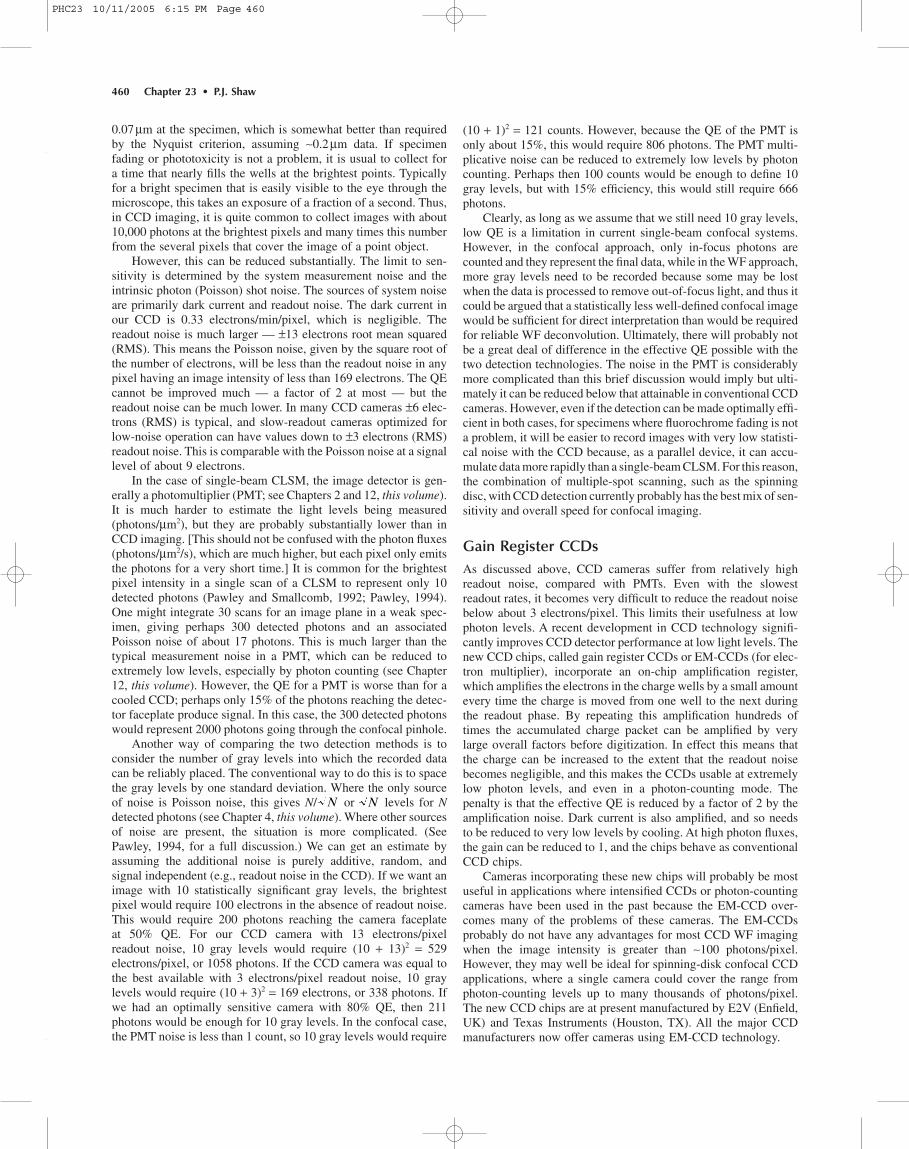
Figure 23.6 shows some images from a real biological speci-men (immunofluorescent labeling of a very thin plant cytoskele-ton “footprint”) that attempts to model this situation. Threeconfocal images taken from a through-focal series starting with thein-focus image and spaced by 2 mm are shown in Figure 23.6(A).An equivalent WF series of images of another footprint on thesame slide is shown in Figure 23.6(B). Given the specimen thick-ness (probably well under 1 mm), there should be no out-of-focuslight to contaminate the WF image. The in-focus WF image shouldbe little different from the confocal image. (A 63¥, NA 1.4 objec-tive was used, and the pinhole was set at approximately 3 Airy diskdiameters.) There is surprisingly little difference between thesetwo focal series. This implies that relatively little of the out-of-focus data is eliminated with a detector aperture of this size in aspecimen such as this, because it consists of thin fibers arrangedin a plane and produces large components at high, in-plane spatialfrequencies.

The Best Solution: Deconvolving Confocal DataThe main effect of the confocal optics should be to remove thevery low spatial frequency out-of-focus components. Conversely,this means that with a detector aperture in this size range, there isstill residual degradation by the out-of-focus high frequency com-ponents from nearby planes in just the same way as for WF optics.Unless a very small detector aperture can be used, confocal opticsdo not provide a complete solution to this “high frequency out-of-focus problem.” Because it is almost invariably impossible to usesuch very small detector apertures, deconvolution offers a practi-cable way to improve the fidelity of the high spatial frequencies inboth WF and confocal 3D images. These considerations as well asthe practical examples given below suggest that it will often behelpful, or even necessary, to apply deconvolution to confocal datato obtain the best resolution of 3D structures. Furthermore, inimages where the pixel spacing is smaller than the Nyquist fre-quency, any spatial frequencies present in the image beyond theNyquist frequency should be removed before the image is dis-played. This is because any such high spatial frequencies cannotcontain meaningful information, and may confuse interpretation ofthe image.

PHC23 10/11/2005 6:15 PM Page 461


As another way of looking at this aspect of the comparisonbetween WF and confocal imaging, consider again the respectivePSFs and OTFs (see Figs. 23.2–23.4). The confocal PSF has muchreduced subsidiary maxima (see Figs. 23.2 and 23.3), largely elim-inating the low spatial frequency out-of-focus light. This corre-sponds to the missing cone region of the WF-OTF being “filledin” in the confocal OTF. This reduction of the out-of-focus con-tribution is one effect of deconvolution on the WF data. However,in addition to this, both WF and confocal OTFs imply an attenua-tion of higher spatial frequencies both in-plane and more markedlyin the z-direction. Deconvolution has the effect of compensatingfor this attenuation, in effect sharpening the image.

For most specimens, it seems unlikely that the low spatial fre-quency out-of-focus light can be regarded as carrying much if anyuseful information (i.e., any useful information that is present fora given focal section is likely to be restricted to focal sections veryclose in z: 1–2mm). The net result of the light that is more out offocus being present in WF images must be to increase at least thePoisson noise associated with the measurement of a given in-focussignal.

Although the previous example may seem somewhat atypical,it has features in common with many real specimens. For example,a specimen may consist of isolated regions of bright labeling thatare thin compared to the depth of field and that occur at signifi-cantly different depths. We might describe such a specimen as“punctate” and an example might be fluorescent, in situ hybridizedchromosomes, which typically contain only a few bright spots ator near the resolution limit and at various focal planes. Unless there

is a substantial real background originating from other focalplanes, widefield CCD imaging is likely to be better than confo-cal imaging for this type of specimen with currently availableequipment. There is relatively little out-of-focus light at low spatialfrequencies, so in these circumstances, the QE of the CCD camerawould probably override the disadvantage that it detects low-frequency out-of-focus light. Similar considerations would applyto punctate labeling at the membrane of a cell or organelle.

If, in addition to the thin plane of interest, the specimen haduniform background intensity, B, throughout the rest of its volume,the WF result would become worse as the specimen becomesthicker, and confocal imaging would become better than WFimaging. This is because the intensity from each additional sliceof the background is added in its entirety to all of the WF images.Thus, the S/N decreases linearly with specimen thickness in theWF case, whereas the background is excluded from the confocalimage, and the S/B is largely independent of specimen thickness.Sandison and colleagues (1993) have calculated the effect on S/Nand signal contrast of the confocal out-of-focus light exclusion.Sandison and colleagues (1993) and Inoué (1986) define contrastas the S/B. Ignoring other sources of noise, the Poisson noise forN counts is and the S/N = . In the presence of background,N = S + B and S/N = S/ . As B is increased for a givensignal, both the contrast, S/B, and the S/N decrease. There comesa point when the in-focus signal, S, becomes lost in the Poissonshot noise [ ] produced by both in-focus and out-of-focuslight. According to this argument, in the WF case the background,B, is increased, while the in-focus “signal” S remains the same.

S B+( )

S B+( )NN

A

B

FIGURE 23.6. A series of confocal (A) and WF (B) optical sections of a plant cytoskeleton “footprint” fluorescently labeled with anti-tubulin. The specimenthickness is less than 1 mm. The confocal detector aperture size was approximately 3 Airy units. The spacing between the optical sections was 2 mm. Field width, 37mm. (Specimen courtesy of Dr. Clive Lloyd.)

PHC23 10/11/2005 6:15 PM Page 462


Sandison and colleagues have calculated for model specimens howS, , and B are affected by the size of the detector aper-ture, how confocal imaging compares with WF imaging, and howto determine the detector aperture size which maximizes detectedS/N. This is also covered in Chapter 22.

The results of this type of analysis clearly depend on theassumptions made about the distribution of fluorescent material inthe specimen; similar analyses need to be made for various differ-ent specimen geometries. Furthermore, the detector aperture sizethat maximizes S/N will not in general give the maximum resolu-tion; deconvolution can be used to improve this situation.

PRACTICAL COMPARISONS

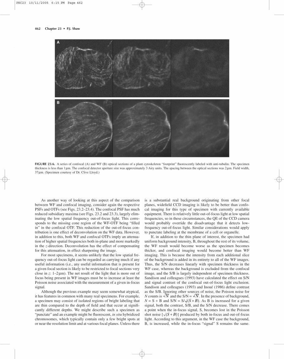
We have undertaken some comparisons of CLSM and CCDimaging of some of the specimens we are using in our work —fluorescent in situ labeling of plant root tip tissue slices ~50mm in thickness (Shaw and Rawlins, 1991b; Highett et al., 1993a,b).Deconvolution can be equally well applied to confocal data, usingthe confocal OTF, to reverse as far as possible the attenuationimplied by these PSF measurements and to substantially reducePoisson noise. Figure 23.7 shows the confocal bead data used toderive the confocal OTF both before [Fig. 23.7(A,C)] and after[Fig. 23.7(B,D)] deconvolution.

In both data sets, deconvolution clearly sharpens the beadimage, particularly in z, and gives some confidence in applying theprocedure to 3D confocal data sets. In Figure 23.8(A–C), the sameportion of a specimen was imaged with three different settings ofthe detector aperture (0.7, 2.5, and 4 Airy units; Shaw and Rawlins,1991b). In each case, a 3D focal section stack of about 30 sectionsseparated by 0.2 mm was collected. A single equivalent sectionfrom these data sets is shown in Figure 23.8. The increase in aper-ture size clearly degrades the resolution. This must be attributedprimarily to contamination of the optical sections with out-of-focus light from nearby parts of the specimen that were too nearfor the detector aperture to eliminate. In each case, the data was

S B+( )deconvolved by the iterative Jansson method, using the appropri-ate PSF measured with the relevant aperture settings. The equiva-lent sections are shown after deconvolution in Figure 23.8(D–F).The deconvolution has restored each image to an equivalent result.Provided the image data has been measured with sufficient accu-racy, deconvolution can restore the different degrees of imagedegradation given by different sizes of detector aperture. Figure23.8(G–L) shows enlargements of the small area boxed in Figure23.8(A). These enlargements show the effect of the deconvolutionalgorithm in reducing the noise in the images.

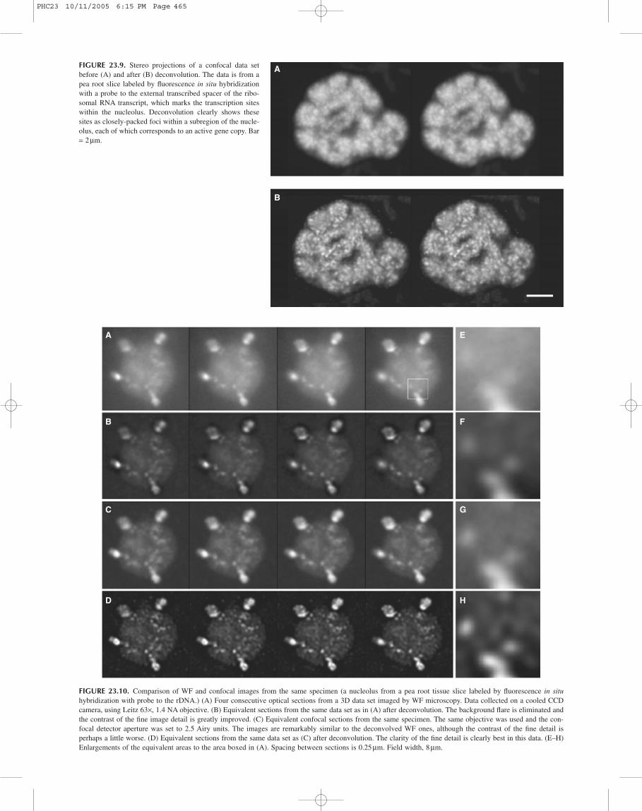
Whatever the relative merits of confocal and WF imaging, itis clear that deconvolution can make good confocal data look evenbetter. Figure 23.9 shows another example of this from our work(Beven et al., 1996). In this image deconvolution clearly resolvesthe labeling of transcription sites within a plant nucleolus to showthat they are composed of many closely-packed foci.

Figure 23.10 shows a specimen imaged by both WF [Fig.23.10(A)] and confocal [Fig. 23.10(C)] microscopy. The agree-ment between the deconvolved WF data [Fig. 23.10(B)] and theraw confocal data [Fig. 23.10(C)] is remarkably good, and givesconfidence that either method will give satisfactory results. Thedeconvolved WF data seems somewhat better than the confocaldata in both x,y and x,z sections. However, the deconvolutionapplied to the confocal data gives the clearest image of all [Fig.23.10(D)].

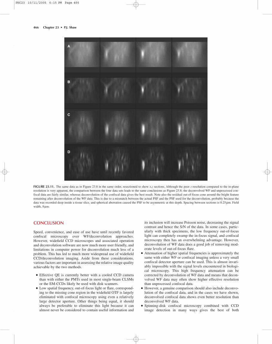
In Figure 23.11, the same data sets are resectioned parallel tothe optical axis (x,z) and lead to very similar conclusions. It shouldbe noted that diverging cones from very bright features are stillvisible after deconvolution of the WF data [arrow in Fig. 23.11(B)].This is because the PSF used in deconvolution is not exactly rightfor the conditions under which the data set was collected. There isclearly considerable spherical aberration, producing an asymmet-rical PSF, possibly because the cell was deep within a tissue slice.Obtaining accurate PSFs for a given specimen is often a substan-tial problem. The ideal solution would be to determine the PSFfrom the data set itself before deconvolution or perhaps to use“blind” deconvolution as described in Chapter 24.

A

B

C

D

FIGURE 23.7. Deconvolution of confocal bead data. (A) x,y sections before deconvolution. (B) x,y sections after deconvolution. (C) x,z sections before decon-volution. (D) x,z sections after deconvolution. (Reproduced from Shaw and Rawlins, 1991b, J. Microsc. 163:151–165.)

PHC23 10/11/2005 6:15 PM Page 463


A B C

D E F

G H I

J K L

FIGURE 23.8. Single equivalent sections from confocal data sets collected with different detector aperture settings before and after deconvolution with theappropriate OTF. (The specimen was a pea root tissue slice labeled by fluorescence in situ hybridization with a probe to the rDNA.) (A–C) Unprocessed con-focal data. (A) Detector aperture, 0.7 Airy units. (B) Detector aperture, 2.5 Airy units. (C) Detector aperture, 4.3 Airy units. (D–F) Equivalent sections to (A–E)after deconvolution. Although the image degradation due to increasing the detector aperture is clear, the reconstructed results are all very similar to each other.(G–L) Enlargements of the equivalent areas from (A–F) to the boxed area in (A), showing the effect of deconvolution on the noise in the image. Field width,12.3mm. (Reproduced from Shaw and Rawlins, 1991b, J. Microsc. 163:151–165.)

PHC23 10/11/2005 6:15 PM Page 464

A

B

FIGURE 23.9. Stereo projections of a confocal data setbefore (A) and after (B) deconvolution. The data is from apea root slice labeled by fluorescence in situ hybridizationwith a probe to the external transcribed spacer of the ribo-somal RNA transcript, which marks the transcription siteswithin the nucleolus. Deconvolution clearly shows thesesites as closely-packed foci within a subregion of the nucle-olus, each of which corresponds to an active gene copy. Bar= 2mm.

A

B

C

D

E

F

G

H

FIGURE 23.10. Comparison of WF and confocal images from the same specimen (a nucleolus from a pea root tissue slice labeled by fluorescence in situhybridization with probe to the rDNA.) (A) Four consecutive optical sections from a 3D data set imaged by WF microscopy. Data collected on a cooled CCDcamera, using Leitz 63¥, 1.4 NA objective. (B) Equivalent sections from the same data set as in (A) after deconvolution. The background flare is eliminated andthe contrast of the fine image detail is greatly improved. (C) Equivalent confocal sections from the same specimen. The same objective was used and the con-focal detector aperture was set to 2.5 Airy units. The images are remarkably similar to the deconvolved WF ones, although the contrast of the fine detail isperhaps a little worse. (D) Equivalent sections from the same data set as (C) after deconvolution. The clarity of the fine detail is clearly best in this data. (E–H)Enlargements of the equivalent areas to the area boxed in (A). Spacing between sections is 0.25 mm. Field width, 8 mm.

PHC23 10/11/2005 6:15 PM Page 465


CONCLUSION

Speed, convenience, and ease of use have until recently favoredconfocal microscopy over WF/deconvolution approaches.However, widefield CCD microscopes and associated operationand deconvolution software are now much more user friendly, andlimitations in computer power for deconvolution much less of aproblem. This has led to much more widespread use of widefieldCCD/deconvolution imaging. Aside from these considerations,various factors are important in assessing the relative image qualityachievable by the two methods.

• Effective QE is currently better with a cooled CCD camerathan with either the PMTs used in most single-beam CLSMsor the EM-CCDs likely be used with disk scanners.

• Low spatial frequency, out-of-focus light or flare, correspond-ing to the missing cone region in the widefield OTF is largelyeliminated with confocal microscopy using even a relativelylarge detector aperture. Other things being equal, it shouldalways be preferable to eliminate this light because it canalmost never be considered to contain useful information and

its inclusion will increase Poisson noise, decreasing the signalcontrast and hence the S/N of the data. In some cases, partic-ularly with thick specimens, the low frequency out-of-focuslight can completely swamp the in-focus signal, and confocalmicroscopy then has an overwhelming advantage. However,deconvolution of WF data does a good job of removing mod-erate levels of out-of-focus flare.

• Attenuation of higher spatial frequencies is approximately thesame with either WF or confocal imaging unless a very smallconfocal detector aperture can be used. This is almost invari-ably impossible with the signal levels encountered in biologi-cal microscopy. This high frequency attenuation can becorrected by deconvolution of WF data and means that decon-volved WF data may often show higher effective resolutionthan unprocessed confocal data.

• However, a genuine comparison should also include deconvo-lution of the confocal data, and in the cases we have shown,deconvolved confocal data shows even better resolution thandeconvolved WF data.

• Spinning-disk confocal microscopy combined with CCDimage detection in many ways gives the best of both

A

B

C

D

FIGURE 23.11. The same data as in Figure 23.8 in the same order, resectioned to show x,z sections. Although the poor z-resolution compared to the in-planeresolution is very apparent, the comparison between the four data sets leads to the same conclusions as Figure 23.8; the deconvolved WF and unprocessed con-focal data are fairly similar, whereas deconvolution of the confocal data gives the best result. Note also the residual out-of-focus cone around the bright featureremaining after deconvolution of the WF data. This is due to a mismatch between the actual PSF and the PSF used for the deconvolution, probably because thedata was recorded deep inside a tissue slice, and spherical aberration caused the PSF to be asymmetric at this depth. Spacing between sections is 0.25 mm. Fieldwidth, 8 mm.

PHC23 10/11/2005 6:15 PM Page 466


Castleman, K.R., 1979, Digital Image Processing, Prentice-Hall, EnglewoodCliffs, New Jersey.

Highett, M.I., Rawlins, D.J., and Shaw, P.J., 1993a, Different patterns of rDNAdistribution in Pisum sativum nucleoli correlate with different levels ofnucleolar activity, J. Cell Sci. 104:843–852.

Highett, M.I., Beven, A.F., and Shaw, P.J., 1993b, Localization of 5S genes andtranscripts in Pisum sativum nuclei, J. Cell Sci. 105:1151–1158.

Hiraoka Y., Minden, J.S., Swedlow, J.R., Sedat, J.W., and Agard, D.A., 1989,Focal points for chromosome condensation and decondensation fromthree-dimensional in vivo time-lapse microscopy, Nature 342:293–296.

Hiraoka, Y., Sedat, J.W., and Agard, D.A., 1988, The use of a charge-coupleddevice for quantitative optical microscopy of biological structures, Science238:36–41.

Hiraoka, Y., Sedat, J.W., and Agard, D.A., 1990, Determination of three-dimen-sional imaging properties of a light microscope system: Partial confocalbehavior in epifluorescence microscopy, Biophys. J. 57:325–333.

Inoué, S., 1986, Video Microscopy, Plenum Press, New York.Jansson, P.A., Hunt, R.M., and Plyler, E.K., 1970, Resolution enhancement of

spectra, J. Opt. Soc. Am. 60:596–599. Pawley, J.B., 1994, The sources of noise in three-dimensional microscopical

data sets, In: Three-Dimensional Confocal Microscopy: Volume Investi-gation of Biological Specimens (J.K. Stevens, L.R. Mills, and J.E. Trogadis, eds.), Academic Press, New York, pp. 48–94.

Pawley, J.B., and Smallcomb, A., 1992, An introduction to practical confocalmicroscopy: The ultimate form of biological light microscopy? ActaMicrosc. 1:58–73.

Petran, M., Hadravsky, M., Egger, M.D., and Galambos, R., 1968, Tandem-scanning reflected light microscope, J. Opt. Soc. Am. 58:661–664.

Sandison, D.R., Piston, D.W., and Webb, W.W., 1993, Background rejectionand optimization of signal-to-noise in confocal microscopy, In: Three-Dimensional Confocal Microscopy: Volume Investigation of BiologicalSpecimens (J.K. Stevens, L.R. Mills, and J.E. Trogadis, eds.), AcademicPress, New York, pp. 211–230.

Self, S.A., 1983, Focusing of spherical Gaussian beams, Appl. Opt.22:658–661.

Shaw, P.J., 1993, Computer reconstruction in three-dimensional fluorescencemicroscopy, In: Electronic Light Microscopy (D. Shotton, ed.), Wiley-Liss,New York, pp. 211–230.

Shaw, P.J., and Rawlins, D.J., 1991a, Three-dimensional fluorescencemicroscopy, Prog. Biophys. Molec. Biol. 56:187–213.

Shaw, P.J., and Rawlins, D.J., 1991b, The point spread function of a confocalmicroscope: Its measurement and use in deconvolution of 3D data, J. Microsc. 163:151–165.

Sheppard, C.J.R., and Choudhury, A., 1977, Image formation in the scanningmicroscope, Opt. Acta. 24:1051–1073.

Stokseth, P.A., 1969, Properties of a defocused optical system, J. Opt. Soc. Am.59:1314–1321.

Wilson, T., 1993, Image formation in confocal microscopy, In: Electronic LightMicroscopy (D.M. Shotton, ed.), Wiley-Liss, New York.

Young, I.T., 1989, Image fidelity: Characterizing the imaging transfer function,Methods Cell Biol. 30:2–47.

Zhang, D.H., Wadsworth, P., and Hepler, P.K., 1990, Microtubule dynamics inliving dividing plant cells: Confocal imaging of microinjected fluorescentbrain tubulin, Proc. Natl. Acad. Sci. U S A 87:8820–8824.

approaches. The confocal optics eliminates much of the out-of-focus light, and its associated noise, and the CCD cameraprovides sensitive and accurate image detection. Parallelimaging at correspondingly lower peak light levels seems tohave definite advantages, particularly for live cells and photo-sensitive specimens. Subsequent deconvolution should havethe effect of increasing the clarity of the image, as it does withdata from a single-beam instrument. This situation can beexpected to improve with the widespread use of EM-CCDs.

SUMMARY

• The relative merits of confocal and WF microscopy depend onthe amount and spatial frequency spectrum of the out-of-focuslight.

• The amount of out-of-focus light depends on the specimen, thedepth distribution of the significant fluorescent intensity, thelevel of generally-distributed non-specific background, and the thickness of the specimen.

• For very thin specimens, or specimens with high fluorescentintensities restricted to thin shells within thick specimens oflow background intensity, there is little out-of-focus light to beexcluded. In these cases, the CCD cameras in use in WFimaging give better QE and therefore statistically better-defined images for a given dose of illuminating photons.

• Image deconvolution should be applied to confocal images aswell as to WF images if the highest resolution is needed andto remove image noise.

ACKNOWLEDGMENTS

This work was supported by the Biotechnology and Biological Sci-ences Research Council of the United Kingdom. I thank JimPawley and Jason Swedlow for stimulating discussions and corre-spondence. I thank Richard Lee for the data shown in Figures 23.2,23.3, and 23.4.

REFERENCES

Agard, D.A., and Sedat, J.W., 1983, Three-dimensional architecture of a poly-tene nucleus, Nature 302:676–681.

Agard, D.A., Hiraoka, Y., Shaw, P.J., and Sedat, J.W., 1989, Fluorescencemicroscopy in three dimensions, Methods Cell Biol. 30:353–378.

Aikens, R.S., Agard, D.A., and Sedat, J.W., 1989, Solid state imagers formicroscopy, Methods Cell Biol. 29:291–313.

Beven, A.F., Lee, R., Razaz, M., Leader, D.J., Brown, J.W., and Shaw, P.J.,1996, The organization of ribosomal RNA processing correlates with thedistribution of nucleolar snRNAs, J. Cell Sci. 109:1241–1251.

PHC23 10/11/2005 6:15 PM Page 467

comparison of wideﬁeld/deconvolution and confocal ... · dimensional (3d) image, or to exclude...

Documents