methods for fuzzy classification and accuracy … for fuzzy classification and accuracy assessment...

Methods for fuzzy classification and accuracy assessment of historicalaerial photographs for vegetation change analyses. Part I: Algorithm

development

F. OKEKE and A. KARNIELI

The Remote Sensing Laboratory, Jacob Blaustein Institute for Desert Research, Ben

Gurion University of the Negev, Sede Boker Campus 84990, Israel;

e-mail: [email protected]

(Received 18 December 2003; in final form 17 February 2005 )

Image classification of historical aerial photographs is very useful for the study of

medium-to-long term (10–50 years) vegetation changes. To determine the quality

of information derived from the classification process, accuracy assessment of the

classification is implemented. Error matrix, which is primarily used in remote

sensing for accuracy assessment, is typically based on an evaluation of the

derived classification against some ‘ground truth’ or reference dataset.

Regrettably ‘ground truths’ for some old historical photographs are rarely

available. To solve this problem we formulate, in this Part I, methods of

classification of aerial photographs and computation of accuracy assessment

parameters of classification products in the absence of ground data, using the

fuzzy classification technique. In addition, since point estimates of these accuracy

parameters require associated standard errors, in order to be useful for statistical

analysis, the method of computation of standard errors of accuracy measures

using the bootstrap resampling techniques is presented. These methods are tested

with historical aerial photographs, of part of Adulam Nature Reserve, Israel,

spanning a period of 51 years. Results illustrate the applicability and efficiency of

the proposed methods.

1. Introduction

Historical aerial photographs have much longer temporal history than satellite-

derived data, and offer the potential for more detailed landscape ecological

assessments. They provide a much longer time frame for assessing the magnitude of

change and for predicting change based on long-term trends (Lo 1986). Aerial

photographs have been available for, at least, the past five decades for most part of

the world. In addition, aerial photographs have high spatial resolution and therefore

offer the possibility of providing more detailed local and regional vegetation

information. Most importantly, the advances in digital photogrammetry, digital

image processing, and geographic information systems (GIS) have further increased

the potential for the use of historical aerial photographs for vegetation change

analyses. Thus, there has been an increased use of historical aerial photographs for

change analyses. Carmel and Kadmon (1998), Kadmon and Harari-kremer (1999)

compared manual interpretation and digital image processing of panchromatic

aerial photographs. They found the accuracy to be similar, and stated the

advantages of digital processing over manual processing of aerial photographs for

International Journal of Remote Sensing

Vol. 27, No. 1, 10 January 2006, 153–176

International Journal of Remote SensingISSN 0143-1161 print/ISSN 1366-5901 online # 2006 Taylor & Francis

http://www.tandf.co.uk/journalsDOI: 10.1080/01431160500166540

change analysis. Others studies include Hudak and Wessman (1998), Turner et al.

(1996), Turner (1990), Coppedge et al. (2001) and Aaviksoo (1993).

Image classification is performed in order to derive specific information, on the

amount and spatial distribution of various types of land use and land cover, from

remotely sensed data (i.e. satellite imagery, aerial photographs), and is generally

regarded as the process of creating thematic maps from images (Campbell 1996,

Lillesand and Kiefer 2000). Most traditional classification methods are ‘crisp’ or

‘hard’ partitioning, in which every given object is strictly classified into a certain

group. In practice, mixed pixels occur because the pixel size may not be fine enough

to capture detail on the ground necessary for specific applications or where the

ground properties, such as vegetation and soil types, vary continuously, as almost

everywhere. The result of hard classification is one class per pixel, whereby much

information about the memberships of the pixel to other classes is lost. Allowing

pixels to have multiple and partial class membership, in which pure and mixed pixels

are accommodated in the classification process, has generally been the solution of

the mixed pixel problem. This is achieved, among other methods, by soft

classification technique, which assigns a pixel to several land cover classes in

proportion to the area of the pixel that each class covers. Fuzzy c-means algorithm

has been shown in various literatures to be one of the most popular soft

classification techniques (Wu and Yang 2002, Yang et al. 2003).

In order to use the products of classification efficiently, users need to know how

accurate these products are. Classification accuracy assessment is therefore an

important stage in the image classification process. One of the most common ways

of representing accuracy assessment information is in the form of an error matrix, or

contingency table. Construction of an error matrix requires the availability of

reference data or ground truth. Unfortunately, for some practical cases of the

classification of historical aerial photographs, the ground data are not available. For

cases where crisp outputs are required, fuzzy classification partitions can be used to

construct a fuzzy error matrix in the absence of ground data.

This paper addresses the problem of lack of ground data in the classification and

accuracy assessment of aerial photographs for change analysis, and describes methods

of solution using the fuzzy classification technique. Section 2 of this paper describes

fuzzy c-means algorithms, which is one of the most popular soft classification

techniques. Section 3 presents the technique of accuracy assessment of classification

products in the absence of ground data, including the application of the bootstrap

resampling method. Techniques presented in this work are tested using real datasets

described in §4, with programs developed in Matlab version 6.5, and results are

presented in §5. Discussions and conclusions are presented in §6 and §7, respectively.

2. Fuzzy c-means (FCM) algorithms

The soft classification technique, which assigns a pixel to several land cover classes

in proportion to the area of the pixel that each class covers, is one of the methods of

solution of the mixed pixel problem. In the literature on soft classifications the fuzzy

c-mean (FCM) algorithms are the most popular methods (Bastin 1997, Wu and

Yang 2002, Yang et al. 2003).

Like in the hard techniques the unsupervised fuzzy classification method (also

known as fuzzy clustering) does not require an extensive prior knowledge of the area

and unique classes are recognized as distinct units. Foody (2000) showed that

supervised FCM may be used to derive accurate estimates of sub-pixel land cover

154 F. Okeke and A. Karnieli

composition especially when all classes have been defined and included in the

training stage of the classification and that the presence of an untrained class

degrades the accuracy of sub-pixel class composition estimation.

Fuzzy c-mean (FCM) is an unsupervised classification or clustering algorithm

that has been applied successfully to a number of problems involving feature

analysis, clustering and classifier design, such as in agricultural engineering, remote

sensing, astronomy, chemistry, geology, image analysis, medical diagnosis and

shape analysis. It is a clustering algorithm that has commonly been adapted for

supervised classification of remotely sensed imagery (Foody 1996, Atkinson et al.

1997, Deer 1998, Deer and Eklund 2003). The modification from unsupervised to

supervised classification involves the specification of fuzzy means and sometimes

also fuzzy covariance matrices, and requires only a single pass of the data through

the algorithm (Deer 1998, Foody 2000, Deer and Eklund 2003).

The FCM algorithm is based on an iterative optimization of an objective function

Jm, which is the weighted sum of squared errors within groups and is defined as

follows (Bezdek 1981):

Jm U , V ; Xð Þ~Xn

k~1

Xc

i~1

Umik xk{vik k2

A, 1 < m <?, ð1Þ

where U is a fuzzy c-partition of X. X5{x1, x2, …, xn} is a finite dataset in the

pattern space Rs, c is a fixed and known number of cluster, V5(v1, v2, …, vc) g Rcs

with vi g Rs Yi being the cluster prototype or cluster centre of class i, 1(i(c. The

parameter m is the weighting exponent for each fuzzy membership, which

determines the ‘degree of fuzziness’, 1(m,‘. If m51, then the algorithm reduces

to the hard c-means algorithm. U5[uik] g Rcn is referred to as the grade of

membership of xk to the cluster i. uik satisfies the following constraints:

uik[ 0, 1½ �; 1¡i¡c, 1¡k¡n;

Xc

i~1

uik~1; 1¡k¡n;

0 <Xn

k~1

uik < n; 1¡i¡c;

ð2Þ

xk{vik k2A is an inner product induced norm on Rs; A is any (sxs) symmetric positive

definitive matrix. Bezdek (1981) showed that for ||xk2vi||A.0, Yi, Yk, then Jm is

minimized only when m.1, and

vi~

Pn

k~1

uikð Þmxk

Pn

k~1

uikð Þm, 1¡i¡c, ð3Þ

uik~1

Pc

j~1

xk{vik k2A

xk{vjk k2

A

� �1=m~1, 1¡i¡c, 1¡k¡n: ð4Þ

Methods for fuzzy classification and accuracy assessment 155

There are many extensions of the original FCM algorithm. Prominent amongstthem are the Gustaffson-Kessel (GK) algorithm (Gustafson and Kessel 1979), and

Gath-Geva (GG) algorithm (Gath and Geva 1989). In this paper, we use the GK

model for the fuzzy classification process.

In general, FCM algorithms depend on certain assumptions in order to define the

subgroups present in a dataset. These assumptions include the optimal number of

classes, c, the initial centroid values, the initial partition, U0, the optimal fuzzy

exponent, m value, and the iteration termination threshold, e value. The optimal

number of classes, c, may be known a priori or determined by cluster validity

process. Detailed studies of the performance of different validity indices can befound in Pal and Bezdek (1995, 1997), and Geva et al. (2000). However, in this

paper, we determine optimal number of clusters by first partitioning the dataset into

an exaggerated number of clusters. Then by visually verifying different clusters in

Erdas Imagine software, we determine clusters to merge in order to form an optimal

number of clusters.

The fuzzy exponent m must also be chosen in order to implement the FCM

algorithm, and its determination is problematic (Pal and Bezdek 1995, 1997). Many

past works have proposed methods of determining optimal fuzzy exponent m. These

include the procedures proposed in McBratney and Moore (1985) and Choe andJordan (1992). However, many researchers simply use m52 as the ideal fuzzy

exponent. In this paper, we use a new and efficient procedure to determine an

optimal fuzzy exponent. In this procedure, the output of the fuzzy classification is

used to predict the original dataset. Then the fuzzy exponent value that corresponds

to the least distance between the predicted data and the original dataset, for a range

of fuzzy exponent values, becomes the optimal value. This is illustrated by

equation (5) below.

X{ X��~s, s > 0, Vm ð5Þ

where X is the original dataset, X�

is the predicted dataset, and I.I is any suitable

similarity measure or distance metric, such as Euclidean distance, divergence

distance, Bhattacharyya distance or angular separation. The predicted dataset is

obtained by pre-multiplying the membership grades matrix by the class centroidmatrix.

3. Accuracy assessment of the classification of historical aerial photographs

There is no classification created from remote sensing data that can be completely

accurate as errors originate from different sources including the classificationalgorithm itself (Steele et al. 1998, Smits et al. 1999). In order to use the products of

classification efficiently, the user needs to know how accurate these products are.

This therefore necessitated accuracy assessment of the remote sensing classification

process. In remote sensing, accuracy assessment is mandatory (Matsakis et al. 2000,

Foody 2002), and is important for providing information about the quality of the

product of classification as well as furnishing the norms for comparing the

performance of different classification methods.

One of the most common ways of representing accuracy assessment information

is in the form of an error matrix, or contingency table (Congalton 1988, 1991, 1993,Congalton and Green 1998, Binaghi et al. 1999, Nishii and Tanaka 1999, Smits et al.

1999, Lewis and Brown 2001, Foody 2002). Error matrix provides a detailed


assessment of the agreement between the sample reference data and classification

data at specific locations, together with a complete description of the misclassifica-

tions registered for each category. In addition to the valuable role of the error

matrix, a number of descriptive and analytical statistical techniques, based on the

error matrix, have been proposed. These are used for summarizing information and

for obtaining accuracy measures that can meet specific objectives. The most

commonly used are the overall accuracy, user’s and producer’s accuracy, and

various forms of kappa coefficients of agreement. Using an error matrix to represent

accuracy has been recommended by many researchers and is central to accuracy

assessment in remote sensing (Binaghi et al. 1999, Nishii and Tanaka 1999, Smits

et al. 1999, Lewis and Brown 2001, Foody 2002).

However, the error matrix and the derived accuracy measures are appropriate

only for hard classification with the assumption that each element of sample data is

associated with only one class in the classification and only one class in the reference

data (Gopal and Woodcock 1994, Foody 1995, Foody and Trodd 1996, Binaghi

et al. 1999, Matsakis et al. 2000, Woodcock and Gopal 2000). For evaluation of soft

classification, various investigations have been made and many suggestions put

forward, some of which are presented in Gopal and Woodcock (1994), Foody

(1995), Foody and Trodd (1996), Binaghi et al. (1999), Ahlqvist et al. (2000), Jaeger

and Benz (2000), Woodcock and Gopal (2000). The procedures of ‘fuzzy error

matrix’ of Binaghi et al. (1999), ‘fuzzy similarity’ of Jaeger and Benz (2000), and the

method of Ahlqvist et al. (2000) are based on fuzzy logic and also retain the

attractive features and popularity of the confusion matrix. Again, these measures

can be applied when either classification or ground data is crisp, and if both are

crisp, they often reduce to standard measures already in use. In this paper, we apply

the method of ‘fuzzy error matrix’ of Binaghi et al. (1999) for the accuracy

assessment of classification of aerial photographs.

3.1 Building fuzzy error matrix in the absence of ground data

The fuzzy error matrix of Binaghi et al. (1999) is constructed as follows: Let ~Rn be

the set of fuzzy reference data assigned to class n, and ~Cn be a set of fuzzy

classification data assigned to class m, with 1(n(Q, 1(m(Q, and Q as the

number of classes. The fuzzy partitions ~Rnand ~Cm are partitions of the dataset X,

and their membership functions are

u ~Rn:X? 0, 1½ �, ð6Þu ~Cm:X? 0, 1½ �, ð7Þ

where [0,1] denotes the interval of real numbers from 0 to 1 inclusive. The fuzzy

error matrix is then given as

~M m, nð Þ~ ~Cn\~Rn

�� ~X

x[X

u ~Cm\

~Rn

xð Þ: ð8Þ

Where the ‘min’ operator is introduced for the intersection operation as

u ~Cm\ ~Rnxð Þ~min u ~Cm

xð Þ, u ~Rm

xð Þ� �

: As in the conventional error matrix, the fuzzy

error matrix can be used to compute descriptive statistics such as the overall

accuracy, producer’s accuracy, user’s accuracy, and kappa coefficient.

The construction of the error matrix requires a reference data or ground truth. In

most of the literature, it is assumed that the ground or reference data used in the


assessment of classification accuracy are themselves accurate representations of

reality (Foody 2002). Actually, the ground data are just another classification which

may contain error (Congalton and Green 1998, Zhou et al. 1998, Lunetta et al. 2001,

Foody 2002). Again the certainty with which a label can be attached to a class is

often based on highly subjective interpretations (Thierry and Lowell 2001, Foody

2002). Therefore, it may be inappropriate to use the term ‘truth’ when describing

ground data (Bird et al. 2000, Foody 2002). Thus, the accuracy assessment referred

to in the foregoing may best be described as measuring the degree of agreement or

correspondence to the ground data and are not necessarily a true reflection of the

closeness to reality (Foody 2002).

Reference data are usually collected from data sources that are assumed to be

more accurate and precise than the data to be classified. Aerial photography is often

used as reference source data for accuracy assessment of classification of satellite

imagery (Congalton and Green 1998). For the classification of aerial photographs

themselves, a ground survey may be the only reliable method of reference data

collection. Unfortunately, in some practical cases, the ground survey cannot be

undertaken since the aerial photographs were collected many years before the study.

Example of such cases are studies where historical aerial photographs, dating back

to many decades, are used for vegetation change analysis and/or studies of certain

temporal ecological processes, and where classification algorithms are used for

labelling different classes of the domain of interest. A ground survey for such cases

cannot be carried out as a long time has elapsed since the data was collected. In cases

where it is not possible to provide ground data, such as in the classification of

historical aerial photographs, researchers often resort to different ad hoc

approaches, which place heavy reliance on the capability of the analyst to interpret

and identify classes of the domain. For instance, in Carmel and Kadmon (1998),

training data for a photograph, where ground data was not available, was generated

by measuring the height of individual shrubs and trees, based on a stereo image of

the photograph.

For cases where crisp outputs are required, fuzzy classification partitions can

be used to solve this problem by providing a means to assess the accuracy of the

crisp products. This idea was first illustrated in Wang (1990a, b). The idea of

using fuzzy partition to assess the accuracy of crisp classification output is based

on the assumption and assertion that membership grade of fuzzy partition

is proportional to the percentage to which the pixel contains a given type of

land cover (Wang 1990a, b). Thus, the fuzzy partition matrix is regarded as more

accurate and precise than its hard counterpart. Other studies have all suggested,

with varying degrees of empirical support, that there is a strong relationship between

fuzzy memberships and true proportions of ground cover. These include Fisher

and Pathirana (1990), Foody (1992a, 1994, 1996), Foody and Cox (1994), Maselli

et al.(1996), Atkinson et al. (1997), Canters (1997), Deer (1998), and Deer and

Eklund (2003). However, Schowengerdt (1996) cautioned against the use of

likelihood indicators (fuzzy memberships derived partly using hard statistical

pattern classification approaches) as a global measure of class mixing proportions,

especially for classes having relatively low separability and considerable distribution

overlap. Also Deer and Eklund (2003) pointed out some cases where

fuzzy memberships did not equal class proportion. Excluding these special cases,

it is generally accepted and assumed that fuzzy partitions have strong correlation

with true class mixing proportions. Based on this assumption, we present in


this paper a method of constructing the fuzzy error matrix in the absence of

ground data.

Let us consider a situation where the crisp product of the classification procedure is

desired. After the fuzzy classification of the dataset is performed, the fuzzy partition is

transformed to a crisp partition by the process of defuzzification. Generally, in remote

sensing, the defuzzification process is performed by assigning the elements of the fuzzy

partition to the class to which they have the highest probability or the highest

possibility of belonging (Matsakis et al. 2000). Let~U~ ~uið Þ, i [ 1 . . . c be a fuzzy

partition of dataset X, then the crisp partition~V~ ~við Þ, i [ 1 . . . c of the dataset X is the

result of defuzzification of~U such that:

~vjk~1[~ujk~max ~uji 1¡i¡cj

� �,

0[~ujk=max ~uji 1¡i¡cj� �

:

(ð9Þ

Using equation (8) the fuzzy error matrix is constructed by taking the crisp partition~V

as the classification partition and the fuzzy partition~U as the reference partition.

~M~ ~V\~U�� ~

X

x[X

u ~V\~

Uxð Þ: ð10Þ

Once the fuzzy error matrix is constructed, other descriptive and analytical statistics

are computed as in the case of the traditional error matrix.

3.2 Estimates of variances and confidence intervals for measures of classificationaccuracy

Table 1 is an example of an error matrix that effectively summarizes the key

information obtained from comparing the classification and reference data. The error

matrix represents a table in which the diagonal entries represent correct classifications,

or agreement between the classification and reference data, and the off-diagonal

entries represent misclassifications, or lack of agreement between the classification

and reference data. In remote sensing, a variety of measures have been suggested for

describing the accuracy of classification from the error matrix (Congalton 1991,

Stehman 1997a, b, Congalton and Green 1998, Stehman and Czaplewski 1998). These

include the overall proportion of area, pixel or polygon classified correctly for the

entire area, various forms of kappa (k) coefficient of agreement, conditional kappa,

user’s and producer’s accuracy. In table 1, pij is theproportion of area in classified

land-cover class i and reference land-cover class j, piz~Pc

j~1

pij is the proportion of

area classified into land cover class i, and pzj~Pc

i~1

pij is the reference proportion of

area in land cover class j.

Table 1. Example of error matrix for a land cover scheme of c classes.

Reference

Classification 1 2 … c1 p11 p12 … p1c p1 +2 p21 p22 … p2c p2 +A A A A A Ac pc1 pc2 … pcc pc +

p + 1 p + 2 … p + c


Definitions of some of these accuracy measures based on the developments in

Congalton (1991, 1993), Stehman (1997a, b), Congalton and Green (1998), Stehman

and Czaplewski (1998) follow.

1. Overall proportion of area correctly classified,

Po~Xc

k~1

Pkk:ð11Þ

2. Kappa,

k~

Po{Pc

k~1

PkzPzk

1{Pc

k~1

PkzPzk

: ð12Þ

3. Kappa with random chance agreement,

ke~Po{1=c

1{1=c: ð13Þ

4. User’s accuracy for class i,

PUi~Pii

Piz

: ð14Þ

5. Producer’s accuracy for cover type j,

PAj~Pjj

Pzj

: ð15Þ

6. The conditional Kappa for the map classification category (row) i,

ki~Pii{PizPzi

Piz{PizPzi

~PUi{Pzi

1{Pzi

: ð16Þ

7. Conditional Kappa for the reference classification in category (column) j,

kj~PAj{Pjz

1{Pjz

: ð17Þ

Though no consensus has been reached on which measures are appropriate for a

given objective of accuracy assessment, the kappa statistic is most often applied in

remote sensing (Stehman 1997b, Congalton and Green 1998, Foody 2002). Stehman

(1997b) showed in detail that no one accuracy measure is universally best for all

accuracy assessment objectives, and proposes criteria for selecting appropriate

accuracy measures for specific study. Congalton and Green (1998) recommended

computation of several accuracy measures since each accuracy measure

reflects different information contained within the error matrix. Also, since

total enumeration of the classified area for verification is at most times impossible,

accuracy assessment of classification of remote sensing data usually requires

sampling of reference data and estimation of parameters describing classification

accuracy. As these accuracy estimates are based on samples, point estimates of these

accuracy parameters clearly require associated standard errors, confidence intervals,

and significant tests in order to be useful for statistical analysis. There are certain


techniques for estimating standard errors and constructing confidence intervals for

measures of classification accuracy derived from the error matrix. One method is to

derive formulas for standard errors of these accuracy measures, based for example,

on large sample methods or a finite population sampling technique, and using the

standard errors estimated to construct confidence intervals based on a normal

distribution assumption (Czaplewski 1994, Stehman 1997a, b, Stehman and

Czaplewski 1998, Blackman and Koval 2000).

The use of derived formulas for standard errors of the accuracy measures,

however, has certain disadvantages. For instance, the formulas derived from the

large sample method can become unreliable as sample size decreases or as kappa

approaches unity (Vierkant 1997). Again the formulas are design-specific and

sometimes may be too complex and difficult to implement. An alternative method of

estimating standard errors of accuracy measures derived from the error matrix is the

application of resampling techniques such as the bootstrap method of Efron and

Tibshirani (1993). This method provides an alternative to large sample techniques

when asymptotic properties are not met or when the standard error of the estimate

has complicated mathematical characteristics (Vierkant 1997). The bootstrap

estimate of standard error requires no theoretical calculations, and is available no

matter how mathematically complicated the estimator may be (Efron and Tibshirani

1993). The bootstrap method has been proposed as a suitable alternative for

constructing confidence intervals about a kappa coefficient in Kalkhan et al. (1997)

and Vierkant (1997).

In this paper, we apply the bootstrap resampling method for the estimation of

standard errors of classification accuracy measures, and the algorithm we use is

described below.

3.2.1 Algorithm for bootstrap estimation of standard errors for classification

accuracy parameters

1. Given a dataset, X5(X1, ..., Xn), perform classification, generate reference

data and classified data (original reference data and original classified data),

construct error matrix, and compute parameters of interest, . Where p is the

number of parameters of interest.

2. 2 Sample with replacement from the reference data and its corresponding

classified data. The number of sample reference data and sample classified

data must be the same as the number of original reference data and original

classified data.

3. Calculate the same parameters of interest using the sample in step 2 to get the

bootstrap replicates, hh�bi , i~1, � � � , p:

4. Repeat steps 2 through 3, B times. Efron and Tibshirani (1993) recommended

a B value of 25 to 200.

5. Estimate the standard error of hhi for each parameter as follows.

cSESEB hhi

� �~

1

B{1

XB

b{1

hh�bi {hh�bi

� �2( )1

2

, ð18Þ

where

hh�bi ~1

B

XB

b~1

hh�bi , Vi: ð19Þ


After the bootstrap standard errors of the parameters of interest have been

computed, confidence intervals can then be constructed based on normal

distribution assumptions (Martinez and Martinez 2002). Confidence intervals are,

however, not constructed in this paper since we used the whole population as the

sample size.

For change detection studies, the computed standard errors of the kappa

coefficients can be used to construct a hypothesis to test for significant differences

between error matrices.

Banko (1998) and Skidmore (1999) describe the test of significance between two

independent kappa’s by the equation

Z~kk1zkk2ffiffiffiffiffiffiffiffiffiffiffiffiffiffiffiffiffiffiffiffiffiffiffiffiffiffiffiffiffiffiffi

s kk1

� �zs kk2

� �r , ð20Þ

where kk1 and kk2 are kappa coefficients for error matrices 1 and 2 respectively,

s kk1

� �, s kk2

� �are standard errors of error matrices 1 and 2 respectively. A null

hypothesis can be set up to test whether the kappa values for the two error matrices

differ significantly.

H0 : k1~k2 versus H0 : k1=k2:

The test for the null hypothesis is performed using the normal curve deviate statistic

(z) and appropriate significance level. This procedure can be applied to paired

combination of error matrices, to determine whether the error matrices differ

significantly (Skidmore 1999).

4. Datasets and methods

4.1 Datasets

Datasets used in testing our proposed methods comprise seven sets of panchromatic

aerial photographs of a section of Adulam Nature Reserve, Israel. The datasets

spanned a period of 51 years, from 1945 to 1996. The aim is to determine

quantitative changes in trees and other vegetation types from 1945 to 1996. There

are no ground data available for these photographs. The photographs are for the

years 1945, 1956, 1967, 1980, 1984 and 1996. All the photographs were scanned with

an A3 UMAX Mirage IIse flatbed scanner at a resolution of 400dpi, into

uncompressed, grey scale tiff format images. For georectification, the digital image

of 1984 was orthorectified using Erdas Imagine software, orthobase module to the

New Israel Grid. Ground control points were provided by a GPS measurement of

selected targets on the image. Using the orthorectified image of 1984 as a reference

image, the remaining set of 1945, 1956, 1965, 1967, 1980, and 1996 were co-

registered to the 1984 orthorectified image. A common subset of area of interest was

extracted for each of the georeferenced data. Since the datasets have different scales

and image sizes, the whole set was further reshaped and resized to a 1 metre

resolution and common image size using programs scripted in Matlab version 6.5.

All the other images were radiometrically normalized to the image of 1945 using the

histogram-matching procedure of Erdas Imagine software. This is aimed at

providing consistent digital number (DN) values for all the dataset.


4.2 Methods

Photo interpretation of the seven datasets revealed three distinct classes that can

easily be identified. These are classes of tress, shrubs and herbaceous plants, and

bare soil. The three classes intermix so much that it was not possible to further

distinguish different classes of trees or shrubs. Fuzzy classification and accuracy

assessment of the seven datasets, in the absence of ground data, are performed by

applying the following steps:

1. The base dataset (1945 dataset) was classified into 10 classes using the fuzzy

algorithm to yield 10 class centroids and a partition matrix. A defuzzification

process is performed to identify pixels that show the highest degree of

belonging to each of the 10 classes. This is equivalent to the traditional hard

classification of the dataset into 10 classes.

2. The hard product is used in Erdas Imagine software environment to visually

identify the classes that most likely belong to the class of trees, shrubs and

herbaceous plants, and bare soil.

3. Using the result of step 2, appropriate classes of the 10 classes are then merged

to form the three major classes of trees, shrubs and herbaceous plants, and

bare soil. The merging procedure was performed by merging class centroids of

appropriate classes and then re-computing the membership grades in a single

pass of the fuzzy algorithm.

4. Using the membership grades obtained in step 3, defuzzification is again

performed to obtain pixels most likely to belong to the three classes of trees,

shrubs and herbaceous plants, and bare soil. Thus we now have a hard

product as well as a fuzzy product of the three classes.

5. Following the procedure described in §3, we take the hard product as the

classification data, and the fuzzy membership grades as the reference data,

and then compute the fuzzy error matrix using equation (10). Using the

computed fuzzy error matrix, accuracy assessment parameters of equa-

tion (11) to equation (17) are computed. Subsequently, the bootstrap

resampling algorithm described in §3 is used to estimate standard errors of

the accuracy assessment parameters, and subsequently other statistical

analysis are performed.

6. The class centroids of the classification of 1945 dataset, obtained in step 3, are

used in a supervised fuzzy classification mode to compute fuzzy membership

grades for each of the rest of the datasets (1956, 1965, 1967, 1980, 1984, and

1996).

7. Steps 4 through 5 are followed for the accuracy assessment of each of the rest

of the datasets.

5. Results

Figure 1 shows hard products of fuzzy classification of the seven datasets. The figure

shows visually, the distribution of trees, shrubs and herbaceous plants, and bare soil

within the area of interest.

Figure 2 shows the percentage coverage of trees, shrubs and herbaceous plants,

and bare soil, for the seven datasets. The figure shows a gradual increase in the

percentage coverage of trees from 1945 till 1996, with a peak period in 1980. The


Figure 1. Hard products of the fuzzy classification of the seven datasets.


percentage coverage of shrubs and herbaceous plants remained fairly constant

between the period 1956 to 1996. A decrease in the percentage coverage of shrubs

and herbaceous plants was observed between 1945 and 1956. Also, the percentage

coverage of bare soil remained constant from 1956 to 1996 with a slight decrease

between 1945 and 1956.

Results of accuracy assessment of the fuzzy classification of the whole datasets

are illustrated in tables 2 to 9 and figures 3 to 12. Tables 2 to 8 show the fuzzy

error matrix for the datasets 1945, 1956, 1965, 1967, 1080, 1984, and 1996

respectively. Close observation of the computed error matrices show con-

siderable off-diagonal elements between trees and shrubs on one hand, and

shrubs and bare soil on the other hand, for all the datasets. These represent a

considerable degree of misclassification if hard products are taken as the final

classification output.

Figure 3 shows the overall accuracy, kappa coefficient (K), and modified kappa

coefficient (Ke) for the whole dataset. All the datasets have higher overall accuracy

values than kappa coefficient values. Overall accuracies for all datasets exceeded

Figure 2. Percentage coverage of the three classes for the seven datasets.

Table 2. Fuzzy error matrix for 1945 dataset.

Reference

Tree Shrubs and herbs Bare soil Row total

Tree 44419.0 3831.5 224.5 48475.0Classification Shrubs and

Herbs2958.6 38457.0 1771.7 43187.0

Bare soil 121.3 1897.0 22880.0 24898.0

Column total 47499.0 44185.0 24876.0


85%, while kappa coefficients for all datasets exceeded 80%. Figure 4 shows the

bootstrap standard deviation of the overall accuracy, kappa coefficient (K), and

modified kappa coefficient (Ke) for the whole dataset. Both kappa coefficients show

higher standard deviations than the overall accuracy.

A null hypothesis was constructed to test whether the error matrices differ

significantly from one another. The result revealed no significant difference between

all paired combinations of the dataset at 0.01, 0.05, and 0.1 significant levels. The


Reference



herbs3782.8 35271.0 2671.5 41725.0

Bare soil 126.8 1287.7 19424.0 20839.0

Column total 53776.0 40309.0 22475.0


Reference



herbs3371.0 34634.0 2014.7 40020.0

Bare soil 175.1 1987.6 20237.0 22400.0

Column total 53438.0 40488.0 22635.0


Reference



herbs3875.6 35325.0 2485.1 41686.0

Bare soil 129.9 1360.1 19112.0 20602.0

Column total 54406.0 40187.0 21967.0


Reference



herbs3953.3 35323.0 2561.6 41838.0

Bare soil 135.7 1405.6 19507.0 21048.0

Column total 53788.0 40334.0 22438.0


computed z statistic for testing significant differences between paired combinations

of fuzzy error matrices for the whole dataset is listed in table 9.

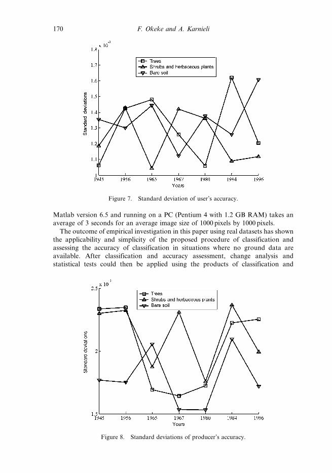
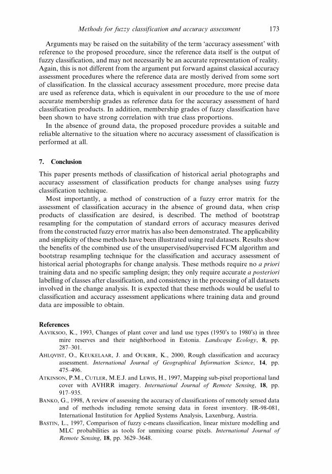
User’s accuracy, producer’s accuracy, estimated standard deviations of the user’s

accuracy and producer’s accuracy for the whole datasets are shown in figures 5 to 8

respectively. Also, conditional kappa coefficients and their corresponding standard

deviations for the whole datasets are shown in figures 9 to 12. In all, trees and bare

soil recorded higher accuracies than shrubs and herbaceous plants. This is attributed


Reference



herbs2575.2 34666.0 2621.7 39863.0

Bare soil 131.5 1307.8 19867.0 21306.0

Column total 52818.0 40815.0 22928.0


Reference



herbs3559.5 34616.0 2807.4 40983.0

Bare soil 115.7 1166.6 19249.0 20531.0

Column total 53933.0 40152.0 22475.0

Figure 3. Overall accuracy and kappa coefficients for the seven datasets.


to the fact that the classes of trees and bare soil have less mixture than the class of

shrubs and herbaceous plants.

6. Discussion

The method described in this paper relies on classification into broad classes using

reflectance from individual pixels, and has been tested with a small number of

classes. The application of this method for complex land cover categorization has

not, however, been tested, but must naturally follow the same procedure as

described here. Surely, the fuzzy classification technique has been successfully

applied to complex land cover categorization. However, a potential difficulty might

arise in very complex land cover cases where the values of class centroids of some

classes are very close. In such cases adequate care must be taken in the

determination of appropriate class centroids for the different categories by using

suitable heuristic techniques in combination with a powerful image display system

(i.e. Erdas Imagine software) to achieve very precise labelling of the classes in the

complex scenario.

Figure 4. Standard deviations for the overall accuracy and kappa coefficients.

Table 9. Z statistics for testing significant differences between paired combinations of fuzzyerror matrices for the whole dataset.

1945 1956 1965 1967 1980 1984 1996

1945 – 0.425 0.401 0.344 0.344 0.516 0.3701956 – 20.006 20.079 20.079 0.123 20.0341965 – 20.069 20.069 0.124 0.0271967 – 0.000 0.196 0.0411980 – 0.196 0.0401984 – 20.1491996 –


The procedure described in this work is aimed at change detection of scenes

captured by image sensors at different times. Therefore the entire procedure

(classification and accuracy assessment of classification) should be carried out for

each image in order to provide the basis for inter-comparison between one image

and another. Different sites located in the same image share the same characteristics

and properties of that image.

All algorithms used in this work are polynomially bounded and are well solved.

Time complexity of stages described here depends mostly on the size of the image to

be processed. Each component of the analysis processed by programs scripted in

Figure 5. User’s accuracy for the seven datasets.

Figure 6. Producer’s accuracy for the seven datasets.


Matlab version 6.5 and running on a PC (Pentium 4 with 1.2 GB RAM) takes an

average of 3 seconds for an average image size of 1000 pixels by 1000 pixels.

The outcome of empirical investigation in this paper using real datasets has shown

the applicability and simplicity of the proposed procedure of classification and

assessing the accuracy of classification in situations where no ground data are

available. After classification and accuracy assessment, change analysis and

statistical tests could then be applied using the products of classification and

Figure 7. Standard deviation of user’s accuracy.

Figure 8. Standard deviations of producer’s accuracy.


accuracy assessment. It is to be emphasized that the accuracy assessment procedure

proposed in this work is suitable for situations where crisp product of classification

is desired.

The proposed procedure shares the advantages and limitations of unsupervised

classification techniques. In particular, the proposed procedure relies on the

capability of the analyst to provide accurate labelling of classes after classification of

the base dataset. Nevertheless, this is not different from the challenges encountered

in a classical supervised classification procedure, where the analyst is expected to

provide training data and reference data for classification and accuracy assessment

Figure 9. Conditional kappa coefficient (classification) for the seven datasets.

Figure 10. Conditional kappa coefficient (reference) for the seven datasets.


respectively. However, an important issue in the application of the proposed

procedure for change detection analysis is that a high level of consistency is

maintained in the classification and post classification labelling of all the datasets.

Consistency, in this case, is largely enhanced by the application of fuzzy supervised

classification for the rest of the datasets using outputs of classification of the base

dataset.

Figure 11. Standard deviations of conditional kappa (classification).

Figure 12. Standard deviations of conditional kappa (reference).


Arguments may be raised on the suitability of the term ‘accuracy assessment’ with

reference to the proposed procedure, since the reference data itself is the output of

fuzzy classification, and may not necessarily be an accurate representation of reality.

Again, this is not different from the argument put forward against classical accuracy

assessment procedures where the reference data are mostly derived from some sort

of classification. In the classical accuracy assessment procedure, more precise data

are used as reference data, which is equivalent in our procedure to the use of more

accurate membership grades as reference data for the accuracy assessment of hard

classification products. In addition, membership grades of fuzzy classification have

been shown to have strong correlation with true class proportions.

In the absence of ground data, the proposed procedure provides a suitable and

reliable alternative to the situation where no accuracy assessment of classification is

performed at all.

7. Conclusion

This paper presents methods of classification of historical aerial photographs and

accuracy assessment of classification products for change analyses using fuzzy

classification technique.

Most importantly, a method of construction of a fuzzy error matrix for the

assessment of classification accuracy in the absence of ground data, when crisp

products of classification are desired, is described. The method of bootstrap

resampling for the computation of standard errors of accuracy measures derived

from the constructed fuzzy error matrix has also been demonstrated. The applicability

and simplicity of these methods have been illustrated using real datasets. Results show

the benefits of the combined use of the unsupervised/supervised FCM algorithm and

bootstrap resampling technique for the classification and accuracy assessment of

historical aerial photographs for change analysis. These methods require no a priori

training data and no specific sampling design; they only require accurate a posteriori

labelling of classes after classification, and consistency in the processing of all datasets

involved in the change analysis. It is expected that these methods would be useful to

classification and accuracy assessment applications where training data and ground

data are impossible to obtain.

ReferencesAAVIKSOO, K., 1993, Changes of plant cover and land use types (1950’s to 1980’s) in three

mire reserves and their neighborhood in Estonia. Landscape Ecology, 8, pp.

287–301.

AHLQVIST, O., KEUKELAAR, J. and OUKBIR, K., 2000, Rough classification and accuracy

assessment. International Journal of Geographical Information Science, 14, pp.

475–496.

ATKINSON, P.M., CUTLER, M.E.J. and LEWIS, H., 1997, Mapping sub-pixel proportional land

cover with AVHRR imagery. International Journal of Remote Sensing, 18, pp.

917–935.

BANKO, G., 1998, A review of assessing the accuracy of classifications of remotely sensed data

and of methods including remote sensing data in forest inventory. IR-98-081,

International Institution for Applied Systems Analysis, Laxenburg, Austria.

BASTIN, L., 1997, Comparison of fuzzy c-means classification, linear mixture modelling and

MLC probabilities as tools for unmixing coarse pixels. International Journal of

Remote Sensing, 18, pp. 3629–3648.


BEZDEK, J.C., 1981, Pattern Recognition with Fuzzy Objective Function Algorithms (New

York: Plenum Press).

BINAGHI, E., BRIVIO, P.A., GHEZZI, P. and RAMPINI, A., 1999, A fuzzy set-based accuracy

assessment of soft classification. Pattern Recognition Letters, 20, pp. 935–948.

BIRD, A.C., TAYLOR, J.C. and BREWER, T.R., 2000, Mapping national park landscape

from ground, air and space. International Journal of Remote Sensing, 21, pp.

2719–2736.

BLACKMAN, N.J.-M. and KOVAL, J.J., 2000, Interval estimation for Cohen’s kappa as a

measure of agreement. Statistics in Medicine, 19, pp. 723–741.

CAMPBELL, J.B., 1996, Introduction to Remote Sensing, 2nd edn (London: Taylor & Francis).

CANTERS, F., 1997, Evaluating the uncertainty of area estimates derived from fuzzy land-

cover classification. Photogrammetric Engineering and Remote Sensing, 63, pp.

403–414.

CARMEL, Y. and KADMON, R., 1998, Computerized classification of Mediterranean

vegetation using panchromatic aerial photographs. Journal of Vegetation Science, 9,

pp. 445–454.

CHOE, H. and JORDAN, J.B., 1992, On the optimal choice of parameters in a fuzzy c-means

algorithm. Proceedings IEEE International Conference on Fuzzy Systems, San Diego,

California, March 8–12, pp. 349–354.

CONGALTON, R.G., 1988, A comparison of sampling schemes used in generating error

matrices for assessing the accuracy of maps generated from remotely sensed data.

Photogrammetric Engineering and Remote Sensing, 54, pp. 593–600.

CONGALTON, R.G., 1991, A review of assessing the accuracy of classifications of remotely

sensed data. Remote Sensing of Environment, 37, pp. 35–46.

CONGALTON, R.G., 1993, A practical look at the sources of confusion in error matrix

generation. Photogrammetric Engineering and Remote Sensing, 59, pp. 641–644.

CONGALTON, R.G. and GREEN, K., 1998, Assessing the Accuracy of Remotely Sensed Data:

Principles and Practices (New York: Lewis Publishers).

COPPEDGE, B.R., ENGLE, D.M., FUHLENDORF, S.D., MASTERS, R.E. and GREGORY, M.S.,

2001, Landscape cover type and pattern dynamics in fragmented southern Great

Plains grasslands, USA. Landscape Ecology, 16, pp. 677–690.

CZAPLEWSKI, R.L., 1994, Variance approximations for assessments of classification accuracy.

RM-316, USDA, Forest Service, Rocky Mountain Forest and Range Experiment

Station, Fort Collins, Colorado.

DEER, P.J., 1998, Change detection using fuzzy post classification comparison. PhD thesis,

Department of Computer Science, The University of Adelaide, Australia.

DEER, P.J. and EKLUND, P., 2003, A study of parameter values for a Mahalanobis distance

fuzzy classifier. Fuzzy Sets and Systems, 137, pp. 191–213.

EFRON, B. and TIBSHIRANI, R.J., 1993, An Introduction to the Bootstrap (New York:

Chapman and Hall).

FISHER, P.F. and PATHIRANA, S., 1990, The evaluation of fuzzy membership of land cover

classes in the suburban zone. Remote Sensing of Environment, 34, pp. 121–132.

FOODY, G.M., 1992, A fuzzy sets approach to the representation of vegetation continua from

remotely sensed data: an example from Lowland Heath. Photogrammetric Engineering

and Remote Sensing, 58, pp. 221–225.

FOODY, G.M., 1994, Ordinal-level classification of sub-pixel tropical forest cover.


FOODY, G.M., 1995, Cross-entropy for the evaluation of the accuracy of a fuzzy land cover

classification with fuzzy ground truth. ISPRS Journal of Photogrammetry and Remote

Sensing, 50, pp. 2–12.

FOODY, G.M., 1996, Approaches for the production and evaluation of fuzzy land cover

classification from remotely-sensed data. International Journal of Remote Sensing, 17,

pp. 1317–1340.


FOODY, G.M., 2000, Estimation of sub-pixel land cover composition in the presence of

untrained classes. Computers and Geosciences, 26, pp. 469–478.

FOODY, G.M., 2002, Status of land cover classification accuracy assessment. Remote Sensing

of Environment, 80, pp. 185–201.

FOODY, G.M. and COX, D.P., 1994, Sub-pixel land-cover composition estimation using a

linear mixture model and fuzzy membership functions. International Journal of

Remote Sensing, 15, pp. 619–630.

FOODY, G.M. and TRODD, N.M., 1996, Representation of ecological trends in remotely

sensed data: relating the probability of class membership to canopy composition and

vegetation ordination. Geocarto International, 11, pp. 3–11.

GATH, I. and GEVA, A.B., 1989, Unsupervised optimal fuzzy clustering. IEEE Transactions of

Pattern Analysis and Machine Intelligence, 11, pp. 773–781.

GEVA, A.B., STEINBERG, Y., BRUCKMAIR, S. and NAHUM, G., 2000, A comparison of cluster

validity criteria for a mixture of normal distributed data. Pattern Recognition Letters,

21, pp. 511–529.

GOPAL, S. and WOODCOCK, C., 1994, Theory and methods for accuracy assessment of

thematic maps using fuzzy sets. Photogrammetric Engineering and Remote Sensing, 60,

pp. 181–188.

GUSTAFSON, D.E. and KESSEL, W., 1979, Fuzzy clustering with a fuzzy covariance matrix.

Proceedings IEEE-CDC, San Diego, California, January 10–12, pp. 761–766 (New

York: IEEE).

HUDAK, A.T. and WESSMAN, C.A., 1998, Textural analysis of historical aerial photography to

characterize woody plant encroachment in South African savanna. Remote Sensing of

Environment, 66, pp. 317–330.

JAEGER, G. and BENZ, U., 2000, Measures of classification accuracy based on fuzzy similarity.

IEEE Transactions on Geoscience and Remote Sensing, 38, pp. 1462–1467.

KADMON, R. and HARARI-KREMER, R., 1999, Studying long-term vegetation dynamics using

digital processing of historical aerial photographs. Remote Sensing of Environment,

68, pp. 164–174.

KALKHAN, M.A., REICH, R.L. and CZAPLEWSKI, R.L., 1997, Variance estimates and

confidence intervals for the kappa measure of classification accuracy. Canadian

Journal of Remote Sensing, 23, pp. 246–252.

LEWIS, H.G. and BROWN, M., 2001, A generalized confusion matrix for assessing area

estimates from remotely sensed data. International Journal of Remote Sensing, 22, pp.

3223–3235.

LILLESAND, T.M. and KIEFER, R.W., 2000, Remote Sensing and Image Interpretation, 4th edn

(New York: John Wiley and Sons).

LO, C.P., 1986, Applied Remote Sensing (New York: Longman Scientific and Technical).

LUNETTA, R.S., IIAMES, J., KNIGHT, J. and CONGALTON, R.G., 2001, An assessment of

reference data variability using a virtual field reference database. Photogrammetric

Engineering and Remote Sensing, 63, pp. 707–715.

MARTINEZ, W.L. and MARTINEZ, A.R., 2002, Computational Statistics Handbook with Matlab

(New York: Chapman & Hall/CRC).

MASELLI, F., RODOLF, A. and CONESE, C., 1996, Fuzzy classification of spatially degraded

Thematic Mapper data for the estimation of sub-pixel components. International

Journal of Remote Sensing, 17, pp. 537–551.

MATSAKIS, P., ANDREFOUET, S. and CAPOLSINI, P., 2000, Evaluation of fuzzy partitions.

Remote Sensing of Environment, 74, pp. 516–533.

McBRATNEY, A.B. and MOORE, A.W., 1985, Application of fuzzy sets to climatic

classification. Agricultural and Forest Meteorology, 35, pp. 165–185.

NISHII, R. and TANAKA, S., 1999, Accuracy and inaccuracy assessments in land-cover

classification. IEEE Transactions on Geoscience and Remote Sensing, 37, pp. 491–498.

PAL, N.R. and BEZDEK, J.C., 1995, On cluster validity for the fuzzy c-means model. IEEE

Transactions on Fuzzy Systems, 3, pp. 370–379.


PAL, N.R. and BEZDEK, J.C., 1997, Correction to ‘On cluster validity for the fuzzy c-means

model’. IEEE Transactions on Fuzzy Systems, 5, pp. 152–153.

SCHOWENGERDT, R.A., 1996, On the estimation of spatial-spectral mixing with classifier

likelihood functions. Pattern Recognition Letters, 17, pp. 1379–1387.

SKIDMORE, A.K., 1999, Accuracy assessment of spatial information. In Spatial Statistics for

Remote Sensing, A. Stein, F. van der Meer and B. Gorte (Eds) (London: Kluwer

Academic Publishers).

SMITS, P.C., DELLEPIANE, S.G. and SCHOWENGERDT, R.A., 1999, Quality assessment of image

classification algorithms for land-cover mapping: a review and a proposal for a cost-

based approach. International Journal of Remote Sensing, 20, pp. 1461–1486.

STEELE, B.M., WINNE, J.C. and REDMOND, R.L., 1998, Estimation and mapping of

misclassification probabilities for thematic land cover maps. Remote Sensing of

Environment, 66, pp. 192–202.

STEHMAN, S.V., 1997a, Estimating standard errors of accuracy assessment statistics under

cluster sampling. Remote Sensing of Environment, 60, pp. 258–269.

STEHMAN, S.V., 1997b, Selecting and interpreting measures of thematic classification

accuracy. Remote Sensing of Environment, 62, pp. 77–89.

STEHMAN, S.V. and CZAPLEWSKI, R.L., 1998, Design and analysis for thematic map accuracy

assessment; fundamental principles. Remote Sensing of Environment, 64, pp. 331–344.

THIERRY, B. and LOWELL, K., 2001, An uncertainty-based method of photo interpretation.


TURNER, I.M., WONG, Y.K., CHEW, P.T. and IBRAHIM, A., 1996, Rapid assessment of

tropical rain forest successional status using aerial photographs. Biological

Conservation, 77, pp. 177–178.

TURNER, M.G., 1990, Spatial and temporal analysis of landscape patterns. Landscape

Ecology, 4, pp. 21–30.

VIERKANT, R.A., 1997, A SAS macro for computing bootstrapped confidence intervals about

a kappa coefficient. 22nd Annual SAS Users Group International Conference (SAS

Inst. Inc), San Diego, California, March 16–19.

WANG, F., 1990a, Fuzzy supervised classification of remotely sensed images. IEEE

Transactions on Geoscience and Remote Sensing, 28, pp. 194–201.

WANG, F., 1990b, Improving remote sensing image analysis through fuzzy information

representation. Photogrammetric Engineering and Remote Sensing, 56, pp. 1163–1169.

WOODCOCK, C.E. and GOPAL, S., 2000, Fuzzy set theory and thematic maps: accuracy

assessment and area estimation. International Journal of Geographical Information

Science, 14, pp. 153–172.

WU, K.-L. and YANG, M.-S., 2002, Alternative c-means clustering algorithms. Pattern

Recognition, 35, pp. 2267–2278.

YANG, M.-S., HWANG, P.-Y. and CHEN, D.-H., 2003, Fuzzy clustering algorithms for mixed

feature variables. Fuzzy Sets and Systems, 141, pp. 301–317.

ZHOU, Q., ROBSON, M. and PILESJO, P., 1998, On the ground estimation of vegetation cover in

Australian rangelands. International Journal of Remote Sensing, 19, pp. 1815–1820.

176 Methods for fuzzy classification and accuracy assessment

methods for fuzzy classification and accuracy … for fuzzy classification and accuracy assessment...

Documents