meng/msc group task – aircraft
TRANSCRIPT

MEng/MSc group task – Aircraft Group 9
Clémence Carton
Rhodri Davies
Matthew Dryden
Jonathan Fairfoull
Roshenac Mitchell
Kyle Sutherland
26.11.15

Abstract
Having chosen the NACA 2408 aerofoil it was investigated whether this wing could be used effectively on an Airbus A380. The equivalent Joukowski aerofoil was analysed as well as the takeoff, cruising and landing conditions of the Airbus with our chosen NACA aerofoil.

Table of Contents Table of Figures .......................................................................................................................... 41 Introduction ......................................................................................................................... 62 Airfoil .................................................................................................................................. 6
2.1 Joukowski ................................................................................................................... 92.2 NACA 2408 ................................................................................................................ 9
3 Finite Wing ....................................................................................................................... 113.1 Lift Distribution ........................................................................................................ 113.2 Lift Coefficient .......................................................................................................... 123.3 Induced Drag ............................................................................................................. 123.4 Induced Drag Coefficient .......................................................................................... 133.5 Downward wash velocity .......................................................................................... 133.6 Skin Friction ............................................................................................................. 14
3.6.1 Fuselage ............................................................................................................ 143.6.2 Wing .................................................................................................................. 153.6.3 Rear stabilisers .................................................................................................. 16
3.7 Total Drag Coefficient .............................................................................................. 173.7.1 Wing .................................................................................................................. 173.7.2 Stabilisers .......................................................................................................... 17
3.8 Total Drag ................................................................................................................. 184 Boundary Layers ............................................................................................................... 18
4.1 Flat Plate Analysis .................................................................................................... 185 Take-off ............................................................................................................................. 206 Landing ............................................................................................................................. 28
6.1 Approach ................................................................................................................... 286.2 Deceleration .............................................................................................................. 296.3 Drag Forces ............................................................................................................... 316.4 Braking Force ............................................................................................................ 33
7 Power Fuel ........................................................................................................................ 338 Fuel Consumption ............................................................................................................. 349 Conclusion ........................................................................................................................ 3610 Distribution of Work ..................................................................................................... 37Appendices ................................................................................................................................ 39
Appendix A – Finite Wing (b/2) ........................................................................................... 39Appendix B – Aerofoil .......................................................................................................... 40Appendix C – Matlab code for Joukowski Transform .......................................................... 41Appendix D – Total drag coefficient .................................................................................... 45Appendix E ........................................................................................................................... 46
Appendix E.1 – Main Take-off Program .......................................................................... 46Appendix E.2 – Auxiliary Function: Front Wing Drag .................................................... 49Appendix E.3 – Auxiliary Function: Rear Vertical Wing Drag ....................................... 51Appendix E.4 – Auxiliary Function: Rear Horizontal Wing Drag ................................... 53
Appendix F – Landing Matlab code ..................................................................................... 55Appendix F.1 – Landing Excel Spreadsheet ..................................................................... 56

Table of Figures
Figure 2-1: Joukowski Transform ............................................................................................... 6Figure 2.2: Result of the Matlab code ......................................................................................... 7Figure 2.3: Lift coefficient on Joukowski airfoil ........................................................................ 8Figure 3.1: Lift distribution ....................................................................................................... 11Figure 3.2: Induced Drag .......................................................................................................... 12Figure 3.3: Induced drag coefficient ......................................................................................... 13Figure 4.1: Flat plate of an aerofoil .......................................................................................... 20Figure 5.1: Vertical forces and their position across the length of the aircraft. [7] .................. 21Figure 5.2: Free-body diagram showing the forces acting upon the aeroplane. ....................... 22Figure 5.3: Shows the time each engine takes to reach take-off speed ..................................... 25Figure 5.4: Indicates the reduction in acceleration due to increased friction at higher speeds. 26Figure 5.5: Shows the aircraft power with each engine configuration. .................................... 26Figure 5.6: Shows the total potential energy of the engines – kinetic energy of the aircraft ... 27Figure 6-1: Lift Force Against Velocity for Angle Range ........................................................ 28Figure 6-2: Typical Approach of an Aircraft [16] .................................................................... 29Figure 7-1: Take-off condition .................................................................................................. 33Figure B.1: Combined Aerofoil cross-section .......................................................................... 40Figure B.2: Joukowski aerofoil ................................................................................................. 40Figure B.2: NACA aerofoil ....................................................................................................... 40

List of Tables
Table 2.1: Lift and drag cofficients for the Joukowski Airfoil ................................................... 9Table 2.2: Lift and drag cofficients for the NACA 2408 Airfoil .............................................. 10

1 Introduction
This project aimed to design an airfoil for an aircraft. From that design, the aerodynamic aspects of the aircraft were to be obtained to give a complete arrangement.
In order to achieve this, initial conditions had to be set and certain assumptions were made utilising the data available for the Airbus A380:
• Flying from Heathrow to Newark
• Fuselage Length (72.72m)
• Fuselage Width (7.14m)
• Wing Span (79.75m)
• Airfoil Chord Length (11m)
• Cruising Speed (262.5m/s)
• Cruising Altitude (40000ft)
2 Airfoil Identify the Joukowski aerofoil which matches that geometry most closely
By using conformal mapping see figure above, we are able to find the Joukowski aerofoil which matches the best to our NACA profile. Conformal mapping is used in aerodynamics to solve practical aerodynamics application, because by using Joukowski transform the circulation around the cylinder is the same as around the aerofoil.
𝜌𝑉$Γ&'()*+,- = 𝜌𝑉$Γ/0120342)
To help us to solve this problem we have done a Matlab code capable to compare them see Appendix C-1. We have used the same given such as the thickness which is t=0.08 and the parameter related to the camber is c=0.02.
b
a
eb -2b 2b x
y
ξ
ζ z plane w plane
zbzw2
+=
A β
B B A
Figure 2-1: Joukowski Transform

Figure 2.2: Result of the Matlab code
Thanks to this Joukowski transform we are now able to say that the angle 𝛽 = 1.8° and the coordinate of the center of our circle is z=0.02 + 1.08 i
The equation of the offset circle became: 𝑧 = 1.08 ∗ 𝑒)> + 0.02 with 𝜃 = [0; 2𝜋]
Joukowski airfoil lifts coefficient calculation:
𝐶G =8𝜋𝑎𝑐 sin 𝛼 + 𝛽
𝐶G = 0,906𝑤𝑖𝑡ℎ𝑐 ≈ 4𝑎, 𝛼 = 5°𝑎𝑛𝑑𝛽 = 1.8°
See below the results of calculation of lift coefficient with an angle β = 1.8° and with angles of attack varying between -5° and 20°. We can see that the Lift coefficient varies with the angle of attack but the critical angle of attack is close to 13° with this Joukowski airfoil.

Figure 2.3: Lift coefficient on Joukowski airfoil
Now Lift force calculation:
𝐹G = −𝜌𝑉$ΓF] = 4𝜋𝑉$^𝜌𝑎 sin 𝛼 + 𝛽 𝐹G = 85584𝑁𝑝𝑒𝑟𝑢𝑛𝑖𝑡𝑠𝑝𝑎𝑛𝑤𝑖𝑡ℎ𝜌 = 0.3, 𝛼 = 5°, 𝛽 = 1.8°𝑎𝑛𝑑𝑉$ = 262.5𝑚 𝑠
Which means that the global lift force of our Joukowski airfoil applied to A380 is given by:
𝐹G = 79,75 ∗ 85584𝐹G = 6,74 ∗ 10g𝑁
The Force needed to have the plane at equilibrium is𝐹 = 𝑚 ∗ 𝑔 = 5,49. 10g𝑁, its mean that the minimum angle of attack to be at equilibrium is α=3.8°.
-0.6-0.4-0.2
00.20.40.60.81
1.21.4
-10 -5 0 5 10 15 20 25
Cl
Angleofattackβ
LiftcoefficientJoukowskiairfoil
Beta1.8°

2.1 Joukowski
The expected real lift (Cl) and drag coefficient (Cd) were calculated by utilising a software program called ‘JavaFoil’. To calculate the lift and drag coefficient the following values were inserted into the program:
• thickness to chord ratio ij of 8%
• camber to chord ratio kj of 2%
Once the values above were inserted the program, the program calculated the various values at a number of different angle of attacks (α ) and then inserted into a table as shown below in Table 2.2: Lift and drag cofficients for the NACA 2408 Airfoil.
Table 2.1: Lift and drag cofficients for the Joukowski Airfoil
α Cl Cd[°] [-] [-]-5 -0.293 0.04176-4 -0.126 0.03032-3 -0.142 0.01104-2 0.069 0.01042-1 0.291 0.013640 0.512 0.02161 0.732 0.034462 0.949 0.051593 1.135 0.070074 1.264 0.089255 1.278 0.106976 1.4 0.135777 1.575 0.166328 1.752 0.199179 1.924 0.2358210 2.111 0.27256
2.2 NACA 2408
The expected real lift (Cl) and drag coefficient (Cd) were calculated by utilising a software program called ‘JavaFoil’. To calculate the lift and drag coefficient the following values were inserted into the program:
• thickness to chord ratio ij of 8%
• camber to chord ratio kj of 2%
• camber location marked at lkj
40% between the leading edge and the trailing edge

Once the values above were inserted the program, the program calculated the various values at a number of different angle of attacks (α ) and then inserted into a table as shown below in Table 2.2.
Table 2.2: Lift and drag cofficients for the NACA 2408 Airfoil
α Cl Cd
[°] [-] [-]
-5 -0.268 0.03743
-4 -0.133 0.02762
-3 -0.149 0.00894
-2 0.022 0.00829
-1 0.194 0.00819
0 0.366 0.00851
1 0.537 0.00886
2 0.709 0.00939
3 0.88 0.01039
4 1.051 0.01294
5 1.064 0.02811
6 1.161 0.03939
7 1.26 0.05455
8 1.4 0.06432
9 1.544 0.07253
10 1.699 0.07759

3 Finite Wing
3.1 Lift Distribution Real wings are not of an infinite span. They have a finite wing span, because of this it affects the amount of lift generated considerably compared with an infinite wing. To calculate the lift per unit span over the wing the following equations can be utilised:
𝐹G,m = −𝜌𝛤$𝑈$ 1 − mp^
^𝑑𝑧
qrsqr
, N [1]
Where,
𝑈$ = 𝐹𝑟𝑒𝑒𝑠𝑡𝑟𝑒𝑎𝑚𝑣𝑒𝑙𝑜𝑠𝑖𝑡𝑦 = 262.5x4
𝜌 = 𝑑𝑒𝑛𝑠𝑖𝑡𝑦𝑜𝑓𝑎𝑖𝑟𝑎𝑡13000𝑚 = 0.32zx{
𝛤$ = 𝑐𝑖𝑟𝑐𝑢𝑙𝑎𝑡𝑖𝑜𝑛 = −4𝜋𝑈$𝑎 sin(𝛽 + 𝛼)
𝛼 = 𝑎𝑛𝑔𝑙𝑒𝑜𝑓𝑎𝑡𝑡𝑎𝑐𝑘
𝛽 = 𝑏𝑒𝑡𝑎1.8
𝑎 =𝑐ℎ𝑜𝑟𝑑4 =
114 = 2.75
𝑏 = 𝑠𝑝𝑎𝑛𝑜𝑓𝑡ℎ𝑒𝑤𝑖𝑛𝑔 = 79.75𝑚
The elliptical distribution equation above calculates the lift force at a point along the z-axis. Inputting this equation is to a software package such as Excel, can form a graph to give a visual representation of lift distribution, this is shown in the graph below. See Appendix A – Finite Wing (b/2)for the values for each point along the axis.
Figure 3.1: Lift distribution
This equation can be simplified for the whole section to 𝐹G = −𝜌𝛤$𝑈$��𝑏 , which equals
=5222kN at 𝛼 =5 Where,
𝛤$𝑎𝑡5° = −4𝜋𝑈$𝑎 sin 𝛽 + 5 = − 1074

3.2 Lift Coefficient
To calculate the lift coefficient of the wing at a point along the z-axis the following equation is used [2]:
𝐶G,3,l = 𝐹G,m
12 𝜌𝑈$
^𝑐
Where,
C = Chord 11m
The total lift coefficient is calculated by using the following:
𝐶G,4,ji)0* = 𝐹G,4,ji)0*12 𝜌𝑈$
^𝐴×𝜋4 = 0.1217
Where, 𝐹G,4,ji)0* = the total force along the wing.
𝐴�-,� = 11𝑚×80𝑚 = 880𝑚^
3.3 Induced Drag
The induce drag is caused when a moving object redirects the air flow coming at it. The change of direction causes the air to produce a downward force. At the wing tips, the pressure flow changes flow where the differential pressure goes from under the wing to over the wing tip. As a result of this vortices are created. The vortices create a rotational flow which results in a downward direct flow, thus creating induced drag. The equation below calculates the force of induced drag along the z-axis:
𝐹�) = −𝜌 ��^p𝛤$ 1 − m
p^
^𝑑𝑧
qrsqr
, N
This equation is similar to that of the lift distribution equation where if plotted on a graph it will create a parabolic profile, as shown below Figure 3.2: Induced Drag. See appendix Appendix A – Finite Wing (b/2) for the values for each point along the axis.
Figure 3.2: Induced Drag

This induced drag equation can be simplified for the whole section to 𝐹�,) = −𝜌𝛤$^
�� , which
equals -13.6kN at 𝛼 =5
3.4 Induced Drag Coefficient
The induced drag coefficient for the wing at a point along the z-axis can be calculated with the following [2]:
𝐶�,) =𝐶G,3,l^
𝜋𝐴𝑅𝑒 Below shows the induced drag coefficient distribution at each point along the z-axis:
Figure 3.3: Induced drag coefficient
The induced drag for the entire section can be calculated from the following:
𝐶�,) =𝐶G,4,ji)0*^
𝜋𝐴𝑅𝑒 =0.014820.56 = 7.198×10��
Where,
Aspect ratio, 𝐴𝑅 = 4��*j�0-+
= �$x��x
= 2.27
Spanwise efficiency factor, e = 0.9
3.5 Downward wash velocity
The downward wash created from the aerofoil is calculated from the equation below:
V� =��^�= �^��.��
^×�$= −1.78�
� [3]

3.6 Skin Friction
The skin friction force is given by the equation:
𝐹4 =12𝜌𝑈$
^𝐴𝑐k
The following constants are assumed:
𝑈$ =262.5 m/s2 (Cruising speed)
altitude = 40,000 feet
𝜌 = 0.3 𝑘𝑔/𝑚�
𝜇 = 1.4×10�� 𝑘𝑔/𝑚𝑠
To work out the skin friction force for the wings and fuselage the following needs to be calculate:
- Area - Reynolds number (used to identify whether it is lamina or turbulent) - Skin friction coefficient
3.6.1 Fuselage
3.6.1.1 Fuselage length
The fuselage can be viewed as a cylinder, the surface area is calculated as follows:
𝐴 = 𝜋𝐷𝐿
where L = 72.72 and D = 7.14 [4]
Reynolds number can then be used to work out whether the air is turbulent or laminar. This is given by:
𝑅, =𝜌𝑈0𝐿𝜇 =
0.3 ∗ 262.5 ∗ 72.721.4×10�� = 403×10g
Turbulent flow occurs when 𝑅, is greater than 500000. Therefore the fuselage can be assumed to be in turbulent flow.
The following equation is used to work out the skin friction coefficient for turbulent flow

𝑐k =0.0711
𝑅,��
= 1.35×10��
From this it is possible to work out the skin friction force.
𝐹4 =12×0.3×262.5
^×1631.18×1.35×10�� = 22.76𝑘𝑁
3.6.1.2 Cockpit
The cockpit is front facing and leads the aeroplane into incoming air. As the flow is not parallel to the surface; flat plate conditions cannot be assumed. The circulation around the wings was modelled using the Joukowski aerofoil as an approximate shape of the NACA 2408. For the cockpit drag, a bullet is used where the drag coefficient has been determined experimentally.
𝐶+,k14,(�z, = 𝐶+,p1((,i = 0.295[5]
The friction force is applied against the frontal area of the fuselage which is assumed to be circular:
𝐴 = 𝜋𝑟^ = 𝜋7.142
^
= 40.04𝑚^
𝐹4,j0j2�)i =12×0.3×262.5
^×40.04×0.295 = 122.09𝑘𝑁
The total skin friction of the fuselage section is the addition of these two:
𝐹4,k14,(�z, = 122.09 + 22.76 = 144.85𝑘𝑁
3.6.2 Wing
For the wing the area is taken as the area of the top and bottom of the wing. The area is calculated as follows:
𝐴 = 2×𝑠𝑝𝑎𝑛×𝑐ℎ𝑜𝑟𝑑
where span = 79.75 and chord = 11.
Reynolds number can then be used to work out whether the air is turbulent or laminar. This is given by:
𝑅, =𝜌𝑈0𝐿𝜇 =
0.3 ∗ 262.5 ∗ 111.4×10�� = 61×10g
Turbulent flow occurs to occur when 𝑅, is greater than 500000. We can therefor take the wing as being in turbulent flow.

To work out the skin friction coefficient for turbulent flow the following equation is use
𝑐k =0.0711
𝑅,��
= 1.97×10��
The skin friction force can now be calculated.
𝐹4 =12×0.3×262.5
^×1631.18×1.97×10�� = 33.2𝑘𝑁
3.6.3 Rear stabilisers
The Reynolds number under cruising conditions:
𝑅𝑒�0-)m0*i�( =0.3 ∗ 262.5 ∗ 7.51.42×10�� = 4.159×10�
𝑅𝑒�,-i)j�( =0.3 ∗ 262.5 ∗ 9.51.4×10�� = 5.26×10�
Turbulent flow occurs when 𝑅𝑒 is greater than 500000, in both cases we can assume fully turbulent flow, neglecting the initial laminar and transitional regions. The coefficient of skin friction can then be calculated and hence the skin friction:
𝑐k,�0-)m0*i�( =0.0711
𝑅𝑒�0-)m0*i�(��= 0.002126
𝑐k,�,-i)j�( =0.0711
𝑅𝑒�,-i)j�(��= 0.0020274
𝐹4,�0-)m0*i�( =12×𝜌×𝑈$
^×𝐴×𝐶k
Each surface area of the wing is required:
𝐴�0-)m0*i�( = 2×30.37×7.5 = 455.55𝑚^
𝐴�,-i)j�( = 2×14.59×9.5 = 277.21𝑚^
The friction for each stabiliser:
𝐹4,�0-)m0*i�( =12×0.3×262.5
^×455.55×0.002126 = 10.008𝑘𝑁
𝐹4,�,-i)j�( =12×0.3×262.5
^×277.21×0.0020274 = 5.809𝑘𝑁
These stabilisers are symmetric aerofoils, the coefficient of lift is zero for zero angle of attack therefore the induced drag is also zero. The total skin friction for the tail section is simply:
𝐹4,i�)( = 𝐹4,�0-)m0*i�( + 𝐹4,�,-i)j�( = 10.008 + 5.809 = 15.817𝑘𝑁
We can now add these together to get the total skin friction:

𝐹4,i0i�( = 𝐹4,k14,(�z, + 𝐹4,3)*z + 𝐹4,i�)( = 144.85 + 33.2 + 15.817 = 193.87𝑘𝑁
The force required in cruising conditions for each engine is therefore:
𝐹,*z)*, =𝐹4,i0i�(
𝑁𝑜. 𝑜𝑓𝑒𝑛𝑔𝑖𝑛𝑒𝑠 =193.874 = 48.468𝑘𝑁
3.7 Total Drag Coefficient
3.7.1 Wing
The total drag coefficient for the wings is calculated by adding up the following:
𝑇𝑜𝑡𝑎𝑙𝑑𝑟𝑎𝑔𝑐𝑜𝑒𝑓𝑓𝑖𝑐𝑖𝑒𝑛𝑡 = 𝑐k +𝑐� +𝑐+
where
𝑐k = 𝑠𝑘𝑖𝑛𝑓𝑟𝑖𝑐𝑡𝑖𝑜𝑛𝑑𝑟𝑎𝑔𝑐𝑜𝑒𝑓𝑓𝑖𝑐𝑖𝑒𝑛𝑡 𝑣𝑖𝑠𝑐𝑜𝑢𝑠𝑑𝑟𝑎𝑔
𝑐� = 𝑝𝑟𝑒𝑠𝑠𝑢𝑟𝑒𝑑𝑟𝑎𝑔𝑐𝑜𝑒𝑓𝑓𝑖𝑐𝑖𝑒𝑛𝑡(𝑓𝑜𝑟𝑚𝑑𝑟𝑎𝑔)
𝑐+ = 𝑖𝑛𝑑𝑢𝑐𝑒𝑑𝑑𝑟𝑎𝑔𝑐𝑜𝑒𝑓𝑓𝑖𝑐𝑖𝑒𝑛𝑡
The profile drag is given by 𝑐k +𝑐� . Since it is very hard to calculate the pressure drag coefficient, we will get the profile drag from 'Javafoil'. This is given by 0.01039.
The drag coefficient is given by the equation:
𝑐+ =𝑐G^
𝜋×𝐴𝑅×𝑒
where
𝐴𝑅 𝐴𝑠𝑝𝑒𝑐𝑡𝑅𝑎𝑡𝑖𝑜 =𝑠𝑝𝑎𝑛𝑐ℎ𝑜𝑟𝑑 =
79.7511 = 7.25
this is assuming that the wing has a constant chord length.
e is the span efficiency factor. It is possible to assume Oswald efficiency factor = 0.9 [6].
From the table of previously calculated lift coefficient for different wing span, assuming an angle of attack of 3° , the total drag coefficient of the wing can be calculated.
From the appendix D.1 the total drag coefficient of the wing can be seen to be roughly 0.02383.
3.7.2 Stabilisers
In addition to the drag of the wings the fuselage and stabilisers add friction drag:

𝑐+ = 𝑐k +𝑐�
where
𝑐k = 𝑠𝑘𝑖𝑛𝑓𝑟𝑖𝑐𝑡𝑖𝑜𝑛𝑑𝑟𝑎𝑔𝑐𝑜𝑒𝑓𝑓𝑖𝑐𝑖𝑒𝑛𝑡 𝑣𝑖𝑠𝑐𝑜𝑢𝑠𝑑𝑟𝑎𝑔
𝑐� = 𝑝𝑟𝑒𝑠𝑠𝑢𝑟𝑒𝑑𝑟𝑎𝑔𝑐𝑜𝑒𝑓𝑓𝑖𝑐𝑖𝑒𝑛𝑡(𝑓𝑜𝑟𝑚𝑑𝑟𝑎𝑔)
In this case the drag coefficient can be calculated by JavaFoil which required the Reynolds number of the flow around them.
𝑅𝑒�-,�- = 42187500
𝑅𝑒�-,�- = 53437500
𝑐+,�-,�- = 0.0053
𝑐+,�-,�- = 0.0052
3.8 Total Drag
The total drag is the addition of all the components of drag. As the fuselage is not a aerofoil the drag coefficient is not given by JavaFoil and the skin friction equations above are assumed.
𝐹+,j0x�0*,*i = 𝜌𝐶+𝑈$^𝐴j0x�0*,*i 𝐹+,k14,(�z, = 𝐹4,(,*zi� + 𝐹+,k-0*i = 22.7 + 224.2 = 246.9𝑘𝑁
𝐹+,�-,�- = 14.9𝑘𝑁 𝐹+,�-,�- = 25.0𝑘𝑁 𝐹+,3)*z = 94.7𝑘𝑁 𝐹+,)*+1j,+ = 54.4𝑘𝑁
𝐹i0i�( = 246.9 + 14.9 + 25.0 + 94.7 + 54.4 = 455.8𝑘𝑁
4 Boundary Layers
4.1 Flat Plate Analysis
LAMINAR-TURBULENT REGION
Modelling as a flat plate, the laminar-turbulent region and boundary layers of the airfoil section were found.
Onset of the transition region was found from the Reynolds Number equation. Given that the turbulent region begins when Re=360000:
𝑅𝑒� =𝜌𝑈$𝑥�𝜇
𝑥� =360000𝜇𝜌𝑈$

𝑥� =360000 0.0000142
0.3 262.5
𝑥� = 0.0649𝑚
The fully turbulent region occurs when Re=500000:
𝑅𝑒& =𝜌𝑈$𝑥&𝜇
𝑥& =500000𝜇𝜌𝑈$
𝑥& =(500000)(0.0000142)
(0.3)(262.5)
𝑥& = 0.0902𝑚
BOUNDARY LAYER
The Boundary Layers of each region were found assuming a Blasius Profile could be applied. At the end of the Laminar flow:
𝛿G =5𝑅𝑒
𝑥
𝛿G =5
3600000.0649
𝛿G = 0.000541𝑚
Turbulent Flow conditions begin at 0.0902m along the wing length, and the associated boundary layer will grow as the length increases to the maximum chord length of 11m. At the onset of Turbulent Flow:
𝛿�,¡ =0.366𝑅𝑒$.^ 𝑥
𝛿�,¡ =0.366
(500000)$.^ 0.0902
𝛿�,¡ = 0.00239𝑚
For chord length 11m and Re=61000000:
𝑅𝑒 =(0.3)(262.5)(11)
0.0000142 = 61000000
𝛿�,¢ =0.366𝑅𝑒$.^ 𝑥

𝛿�,¢ =0.366
(61000000)$.^ 11
𝛿�,¢ = 0.1116𝑚
The plane itself can be analysed as a flat plate, giving the boundary layer at the tail section:
𝑅𝑒 =(0.3)(262.5)(72.72)
0.0000142 = 403300000
𝛿��)( =0.366
(403300000)$.^ (72.72)
𝛿��)( = 0.506𝑚
Figure 4.1 shows the height of the boundary layer for the airfoil.
Figure 4.1: Flat plate of an aerofoil
5 Take-off
To model the take-off of an aeroplane a kinematic model is considered as shown in Figure 5-1. In order to calculate the equivalent lift requirement of the wing, the moment of each lift force from the force of gravity must be determined. The tail lift and the main wing lift must be balanced against the centre of gravity (CoG) to keep it flying straight. The equilibrium is essential on any aircraft because it ensures the aircraft does not rotate and dive. On passenger aircraft the CoG changes position regularly, generally manufacturers will provide an acceptable range of loading configurations to allow for adaption of the mass centre and the counteracting mechanisms used by the aeroplane such as the rear wing flap deflection.
0.000541m 0.00239m 0.116
m

Figure 5.1: Vertical forces and their position across the length of the aircraft. [7]
The main forces and distances are given below with the following assumptions:
𝐹z = 22.23𝑚, parallel to the inboard engines, measured from the nose. [7]
𝑑� = 7.71𝑚, parallel to the outboard engines, measured from the CoG datum. [7]
𝑑^ = 40.835𝑚, assuming that lift force is uniform from the centre of the wing. [7]
To find the lift requirements of each wing we assume the equilibrium of forces and use Newton’s second law calculate the force:
0𝐹z = 7.71𝐹G,3 + 40.835(−𝐹G,i)
𝐹G,i =7.7140.835𝐹G,3
𝐹z = 𝐹G,3 − 𝐹G,i = 1 −7.7140.835 𝐹G,3 = 0.8112𝐹G,3
𝐹G,3 = 1.2328𝐹z
𝐹z = 𝑚𝑔 = 577000×9.807 = 5659𝑘𝑁
𝐹G,3 = 6976𝑘𝑁
𝐹G,i = 1317𝑘𝑁
The lift required from the wing is used to find the take-off speed of the aircraft. The lift equation can be rearranged for the speed that this lift can be achieved:
𝐹( =12𝜌𝑣i0
^𝑐(,3)*z𝐴3)*z
𝐴 = 𝑙𝑒𝑛𝑔𝑡ℎ𝑥𝑐ℎ𝑜𝑟𝑑 = 79.75×11 = 877.25𝑚
𝐶( = 1.56 at 20 degree flap deflection calculated with JavaFoil [8].
𝐹( = 6976𝑘𝑁
𝜌 = 1.225𝑘𝑔/𝑚� the standard density of air at ground level.

𝑣i�2,�0kk =2𝐹(𝜌𝐴𝑐(
=2×6976000
1.225×877.25×1.56 = 91.23𝑚𝑠��
The take-off speed is the minimum speed at which this aeroplane can provide enough lift to leave the ground. A range is usually given for speeds that are safe to take-off at and the minimum is likely to be higher than this speed to allow for different conditions of take-off. To calculate the thrust force required from the engines to achieve sufficient acceleration, within the limits of the runway, we utilise the fundamental equations of motion. The addition of either a distance or time restriction is required; for most applications a distance is easier to limit as the runway is a set distance. In this case a distance range of 2000 to 3000m coincides with Heathrow and Newark airports which both have runways exceeding 3km [9] [10].
𝑡 =𝑣 − 𝑢𝑎
𝑠 =12𝑎𝑡
^ =𝑎2𝑎^ (𝑣 − 𝑢)
^ =𝑣^
2𝑎
𝐹 = 𝑚𝑎 = 𝑚𝑣^
2𝑠
The engine requirements for: take-off speed achieved at three kilometres and safely within the runway length at two kilometres. The ratio of the forces is the inverse of the ratio of the distances as the force of acceleration is inversely proportional to distance.
For: S = 3000m
𝐹x)* = 57700091.23^
2×3000 = 800.366𝑘𝑁
𝐹x�l =32𝐹x)* =
3×800.3662 = 1.201𝑘𝑁
Under these assumptions four engines of 300.2kN will provide enough power for take-off within two kilometres. The Airbus a380 is available with four of Engine Alliance’s GP7200 engines rated at 311kN each and would provide sufficient thrust force alone for this aircraft also. However, when the free-body diagram Fig. 4.2.2 is analysed, there are some issues with this method.
Figure 5.2: Free-body diagram showing the forces acting upon the aeroplane.
Forces act in both x and y axes in positive and negative directions: lift force is reduced by the weight and the thrust force is reduced by the drag. Allocating 𝐹� as the positive direction of x, the real accelerating force is given as:

𝐹� = 𝐹� − 𝐹+
Where:
𝐹� is the acceleration force,
𝐹i is the combined thrust of all the engines
And, 𝐹+ is the total drag force
The total drag force of the aircraft is very difficult to predict and usually determined experimentally within a wind tunnel using a scale model and non-dimensional fluid analysis. This method is costly and accurate to a certain point. There are other methods used to predict a likely drag force numerically using computer programs that can determine the parasitic drag, the induced drag can be determined mathematically and added to this. The application ‘JavaFoil’ is a Java applet that can be used to determine the flow characteristics of aerofoils and is available for free [8]. Parasitic drag initially is zero but increases with speed of the aircraft because the Reynold’s number of the surrounding flow increases. Using a combination of MatLab and JavaFoil the friction of the aircraft has been modelled as the aircraft accelerates to take-off speed (E). Using the friction for each time the acceleration achieved using certain engine thrust is determined. Thus the time taken to reach the take-off speed and the distance travelled over that time period is also calculated. Using the following assumptions the acceleration, speed, distance and force are shown for three engine configurations: the four of Engine Alliance’s GP 7200 [11] engines used in the Airbus-A380; Engine Alliance’s improved GP7277 [11] engines also used for the Airbus-A380 and four General Electric GE90-115B [12] engines used in the Boeing-777.
𝐹i�2,�0kk = 6976𝑘𝑁
Thrust force:
𝐹i,£¤�^$$ = 4×311 = 1244𝑘𝑁
𝐹i,£¤�^�� = 4×374 = 1496𝑘𝑁
𝐹i,£¢�$ = 4×420 = 1680𝑘𝑁
Dimensions:
𝐿k14,(�z, = 72.72𝑚
𝐿x�)*3)*z = 79.75𝑚
𝐿-,�-�0-)m0*i�( = 30.37𝑚
𝐿-,�-�,-i)j�( = 14.59𝑚
𝐷k14,(�z, = 7.14𝑚
𝑐x�)* = 11𝑚
𝑐-,�-,� = 7.5𝑚
𝑐-,�-,� = 9.5𝑚
The chosen aerofoil is from the NACA series, the 2408. The lift characteristics are shown below with a flap deflection of twenty degrees which yielded high lift whilst maintaining a low drag coefficient:

𝐶( = 0.248 [8]
𝐶(,k(�� = 1.56 [8]
The program starts by calculating the acceleration of the aircraft at time 0 and yields the speed after the first time interval. The speed is used to calculate the Reynolds number of the surrounding flow.
𝑅𝑒 =𝜌𝑈$𝐿𝜇
Where:
𝑈$ = 𝑟𝑒𝑙𝑎𝑡𝑖𝑣𝑒𝑠𝑝𝑒𝑒𝑑𝑜𝑓𝑎𝑖𝑟𝑓𝑙𝑜𝑤
𝜌 = 1.225𝑘𝑔𝑚��
𝜇 = 1.73𝑘𝑔𝑚��𝑠��
𝐿 = 𝑐ℎ𝑜𝑟𝑑𝑙𝑒𝑛𝑔𝑡ℎ
The Reynold’s number of each wing is computed for each speed and a switch is used to find the drag coefficient, previously found by Javafoil, for each value of Re. To find the drag of the fuselage a different technique is used. The front face is compared to a bullet where the drag coefficient is determined experimentally as 0.295 [5]. The length of the fuselage is assumed a flat plate with length πD, the circumference of the fuselage and the coefficient of drag is given by:
𝐶+,k14,(�z, =0.0711𝑅𝑒$.^
As the wing provides lift tip vortices form an induced drag as the aircraft accelerates which increases the coefficient of wing drag with the following dependencies:
𝐶+,) =𝐶(^
𝜋×𝐴𝑅×𝑒 =0.248^
𝜋× 79.7511 ×0.9
= 0.003
Where AR is the aspect ratio of the wings and the Ostwald efficiency factor for the Airbus A380:
𝑒 = 0.9
Using the drag coefficients the drag force is determined at each speed remembering that the area used for the wings is doubled for both top and bottom sections:
𝐹+ =12𝜌𝑈$
^𝐴𝐶+
The total drag force is the addition of each component drag however the landing gear and runway friction have not been included in the program. Instead a twenty percent increase in total drag is assumed for the landing gear form and friction drag including the rolling friction on the runway. The force equation derived from the free body diagram is hence satisfied and the new acceleration calculated:
𝑎 =𝐹� − 𝐹+𝑚

For each second the current lift force that would be generated if the flaps were at 20 degrees is calculated using the lift equation above, however it is reduced by a factor of 0.68 due to the parabolic distribution of force over the finite wing where the tips generate zero lift and the fuselage does not add any lift. Once the lift generated by the wings surpasses 6976kN the program ends with the following results: Fig. 4.2.3, the speed-time graph for each engine; Fig. 4.2.4, the acceleration-time graph for each engine; Fig. 4.2.5, the power-time graph of the engines found by the engine force multiplied by velocity; Fig. 4.2.6, the total energy lost over time found by the drag force times distance travelled.
Figure 5.3: Shows the time each engine takes to reach take-off speed

Figure 5.4: Indicates the reduction in acceleration due to increased friction at higher
speeds.
Figure 5.5: Shows the aircraft power with each engine configuration.

Figure 5.6: Shows the total potential energy of the engines – kinetic energy of the
aircraft
The results from the program indicate that the high powered GE90 engines used for the B-777 result in less power loss than with the GP7200 supplied with the A380. The program has its limitations; it is well documented that Engine Alliance’s engines have brought a superior level of fuel consumption and are highly efficient engines. Therefore the recommend engines for this craft are Engine Alliance’s improved GP7277 engines with a rated power of 374kN with two on each wing, the same configuration used in the A380F.
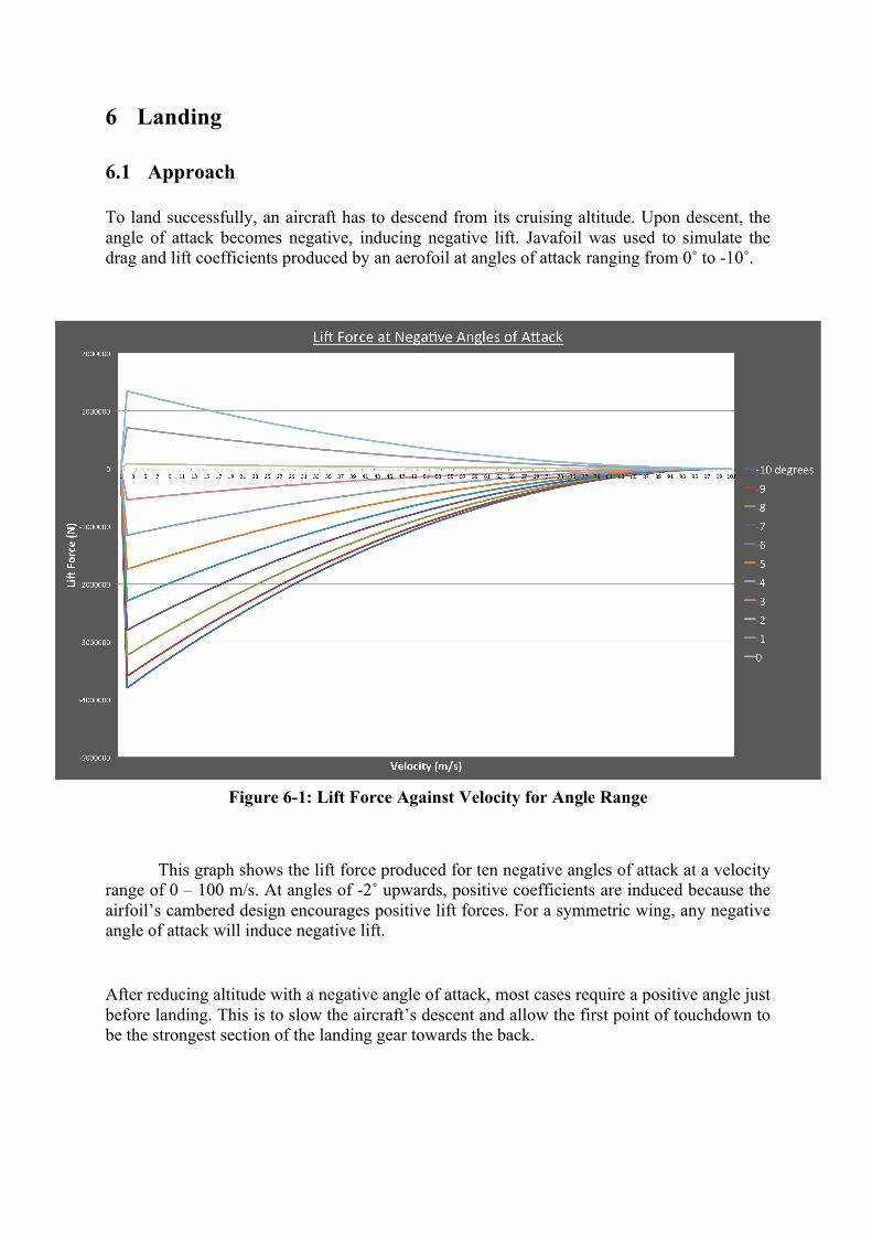
Figure 6-1: Lift Force Against Velocity for Angle Range
6 Landing
6.1 Approach
To land successfully, an aircraft has to descend from its cruising altitude. Upon descent, the angle of attack becomes negative, inducing negative lift. Javafoil was used to simulate the drag and lift coefficients produced by an aerofoil at angles of attack ranging from 0˚ to -10˚.
This graph shows the lift force produced for ten negative angles of attack at a velocity range of 0 – 100 m/s. At angles of -2˚ upwards, positive coefficients are induced because the airfoil’s cambered design encourages positive lift forces. For a symmetric wing, any negative angle of attack will induce negative lift.
After reducing altitude with a negative angle of attack, most cases require a positive angle just before landing. This is to slow the aircraft’s descent and allow the first point of touchdown to be the strongest section of the landing gear towards the back.

6.2 Deceleration
Taking the mass of the aircraft as the maximum an A380 can land with, and using the highest suitable velocity and deceleration upon touchdown, the shortest possible stopping distance has been calculated. All calculations have been simplified by assuming constant acceleration and forces.
Starting with the equation of motion for velocity:
𝑣 =𝑑𝑟𝑑𝑡 = 𝑎𝑡 + 𝑢
𝑑𝑟 = 𝑣. 𝑑𝑡 = 𝑎𝑡 + 𝑢 . 𝑑𝑡
Integrating both sides to find distance travelled:
𝑣. 𝑑𝑡 = 𝑎𝑡. 𝑑𝑡 + 𝑢. 𝑑𝑡
𝑠 = 𝑎𝑡^
2 + 𝑢𝑡
Re-arranging for time:
𝑡^ =2𝑠 − 2𝑢𝑡
𝑎
Squaring equation for velocity to remove the time component:
𝑣 = 𝑎𝑡 + 𝑢
Figure 6-2: Typical Approach of an Aircraft [16]

𝑣^ = 𝑎𝑡 + 𝑢 𝑎𝑡 + 𝑢 = 𝑎^𝑡^ + 𝑢^ + 2𝑡 𝑎. 𝑢
𝑣^ = 𝑎^2𝑠 − 2𝑢𝑡
𝑎 + 𝑢^ + 2𝑡 𝑎. 𝑢
𝑣^ = 2𝑎𝑠 − 2𝑎𝑢𝑡 + 𝑢^ + 2𝑎𝑢𝑡
𝑣^ = 𝑢^ + 2𝑎𝑠
∴ 𝑠 =𝑣^ − 𝑢^
2𝑎
The maximum velocity, weight and deceleration acceptable for a landing A380 have been stated in the Airbus manual. [7] These maximums are related to the landing gear strength and must not be exceeded.
Maximum values for landing:
Approach Velocity Total Mass Deceleration
138 knots (71 m/s) 395,000 kg 3.048 m/s2
𝑎x�l = 3.048𝑚 𝑠^
𝑣 = 71𝑚 𝑠
𝑢 = 0𝑚 𝑠
𝑠x�l = 3353𝑚
Using maximum deceleration, the shortest possible stopping distance:
𝑠x)* =𝑣^ − 𝑢^
2𝑎x�l
𝑠x)* =71^ − 02×3.048 = 826.94𝑚

The associated stopping time for maximum deceleration:
𝑡 =2𝑠 − 2𝑢𝑡
𝑎
𝑡x)* =2×826.94 − 0
3.048 = 23.294𝑠
The minimum required deceleration has been calculated using the length of Newark runway, 3353m. This assumes that the aircraft can use every metre of the runway and is to be taken as an absolute minimum.
𝑠 =𝑣^ − 𝑢^
2𝑎
∴ 𝑎 =𝑣^ − 𝑢^
2𝑠
𝑎 =71^ − 02×3353 = 0.7517𝑚 𝑠^ 𝑑𝑒𝑐𝑒𝑙𝑒𝑟𝑎𝑡𝑖𝑜𝑛.
As the minimum deceleration will have the longest stopping time:
𝑡x�l =2×3353 − 00.7517 = 94.451𝑠
6.3 Drag Forces
Maximum and minimum required forces for each deceleration:
𝐹 = 𝑚𝑎
𝐹x�l,4i0� = 395000×3.048 = 1.2𝑀𝑁(𝑡 = 23.29𝑠)
𝐹x)*,4i0� = 395000×0.7517 = 296.9𝑘𝑁(𝑡 = 94.45𝑠)
Javafoil’s ‘flap deflection’ feature simulates the effect of wing flap position on drag force. A deflection of 20˚ has been applied to the aerofoil to act as a brake after touchdown. A range of values have been calculated using excel but in this example the velocity is 60 m/s:

𝐹+ =12𝐶+𝐴𝜌𝑈$
^
𝐹� = 0.5×0.01384×879.45×1.229×60^ = 49.942𝑘𝑁
Induced drag exists due to lift forces forming vortices around the edges of the aerofoil. For this example AR is 7.25 and e is 0.9. The lift coefficient of the aerofoil with flap deflection 20˚ is 1.968.
𝐶�) =𝐶(,3)*z
^
𝜋𝐴𝑅𝑒
𝐶�) =1.968 ^
𝜋×7.25×0.9 = 0.18894
∴ 𝐹�) = 0.5×0.18894×879.45×1.229×60^ = 367.58𝑘𝑁
The fuselage drag has been calculated using flat plate analysis of the outside area of a cylinder, diameter 7.14m. This is the diameter of the A380 fuselage. The frontal area has been modeled using the drag coefficient of a bullet shape and the same diameter as the fuselage.
𝐹k = 5139.6526 + 26129.597 = 31.26925𝑘𝑁
For this aircraft, the landing gear causes a 20% increase in total drag. Therefore at 60 m/s, shortly after landing, the drag force on the whole aircraft is:
𝐹�,i0i = 1.2× 𝐹k + 𝐹i + 𝐹i3 + 𝐹3,^$ + 𝐹)
𝐹�,i0i = 1.2× 31.27 + 0.656 + 1.729 + 49.942 + 367.583 = 541.42𝑘𝑁

6.4 Braking Force
To find the forward momentum of the aircraft, the force generated during the full deceleration period has been calculated.
𝐹𝑡 = 𝑚�𝑣� − 𝑚^𝑣^
𝐹 =𝑚�𝑣� − 0
𝑡 =395000×71
23.29 = 1.2𝑀𝑁
The brakes used on an A380, Honeywell Carbenix, can produce so much braking force that using reverse engine thrust is not essential to slow the aircraft. [13] At 60 m/s during maximum deceleration, the required braking force for all wheels:
𝐹p-�2, = 𝐹x�l − 𝐹�,i0i
𝐹p-�2, = 1.2𝑀𝑁 − 541.42𝑘𝑁 = 658.59𝑘𝑁
The A380 uses sixteen braked wheels. They are applied at different times while stopping to maintain a smooth deceleration, however for this analysis it is assumed they are all being applied at once.
𝐹p-�2,,)* =𝐹p-�2,16 = 41.16𝑘𝑁
7 Power Fuel
Assuming that for the A380 take-off speed is 280km/h = 77.8 m/s and also during his take-off we will consider a uniform acceleration to simplify calculation.
We will now find the acceleration of the plane during the take-off by considering that the plane needs 50s to do 2000 m in this condition, we have:
Figure 7-1: Take-off condition
V = 0 m/s
D = 0 m
V = 77.8 m/s
D = 2000 m

𝑑𝑉𝑑𝑇 =
𝑉𝑇 =
77.850 = 1.55𝑚/𝑠²
The characteristic equation of the plane during take-off is given by:
𝑑𝑉𝑑𝑇 =
𝐹𝑚 −
𝜌𝑆𝑉²2𝑚 𝐶li�2,0kk − 𝑟𝐶mi�2,0kk − 𝑟𝑔
Where r is the rolling resistance coefficient. It depends of the runway quality. For a paved and dry runway r=0.03. We will consider that there is no wind, we are at sea level and in a standard atmosphere (ρ=1.225).
𝐶mi�2,0kk = 2𝑚𝑔𝜌𝑆𝑉^ =
2 ∗ 560000 ∗ 9.811.225 ∗ 845 ∗ 77.8^ = 1.75
𝐶li�2,0kk = 0.125 = 𝐶𝑧²/(𝑝𝑖𝐴𝑅𝑒)
e=1.01 and AR=7.72
Then we have: 𝐹 = +©+�+ 𝑟 ∗ 𝑔 + ª∗¡∗©r
^∗x𝐶li�2,0kk − 𝑟 ∗ 𝐶mi�2,0kk ∗ 𝑚
𝐹 = 1.24 ∗ 10g𝑁
F give the total force needed to take-off the plane, as we know A380 have 4 engines which means that with this configuration one engine need a minimum of 𝐹 = �.^�∗�$
«
�= 310𝑘𝑁
This means that we will choose 4 GeneralElectric GP7200 as engine for our A380. We know that these four engines consume 2.9 liters for 100km per PAX. A380 is capable to reach 15000km with 853 passengers. Then our typical consumption ratio is 𝐶4 =
^,�∗����$$
=24.7𝐿/𝑘𝑚 which is 12% less than Boeing 747.
8 Fuel Consumption
𝐻𝐶𝑉,-04,*, = 46200𝑘𝐽/𝑘𝑔 [14]
𝜌,-04,*, = 810𝑘𝑔/𝑚�
𝑉x�l,k1,( = 320𝑚�
𝐹+-�z,i0i�( = 456𝑘𝑁
Assuming the A380’s engines (Engine Alliance GP7200) are ideal and cruising at 262.5 m/s for an entire 8-hour flight,
Power required to travel at 262.5 m/s and overcome drag force:
𝑃 = 𝐹𝑣 = 456000 ×262.5 = 119.7𝑀𝑊

Energy required for full flight:
𝐸-,² = 𝑃𝑡 = 119.7×10g × 8×3600 = 3.446×10�𝑘J
Volume of Kerosene burned to produce Ereq:
𝑉k1,(,-,² =𝐸-,²
𝐻𝐶𝑉2,-0𝜌2,-0=3.446×10�
46200×810 = 92.1𝑚� = 92,100𝑙𝑖𝑡𝑟𝑒𝑠
Total mass of burned fuel:
𝑚k1,( = 𝜌k1,(×𝑉k1,( = 810×92.1 = 74,601𝑘𝑔
Mass flow rate for all engines per second of flight at 262.5 m/s:
𝑚 =𝑚k1,(
𝑡k()z�i=
746018×3600 = 2.59𝑘𝑔/𝑠
For each engine:
𝑚 =2.59𝑘𝑔/𝑠
4 = 0.6475𝑘𝑔/𝑠
Fuel consumption (kg/s) per kilo-newton of thrust to overcome skin friction for all engines:
𝑇𝑆𝐹𝐶 =2.59456 = 5.68×10��
𝑘𝑔𝑠 /𝑘𝑁
If the aircraft is at the maximum fuel capacity of 320,000 litres [15] and cruising at 262.5 m/s, the longest possible flight time is:
𝑚k1,( = 𝜌k1,(×𝑉k1,( = 810×320 = 259200𝑘𝑔
𝐸x�l = 𝐻𝐶𝑉2,-04,*,×𝑚k1,( = 46200×259200 = 11.975×10�𝑘𝐽
𝑡 =𝐸𝑃 =
11.975×10�^
105.368×10g = 113649.3𝑠 = 31.57ℎ𝑜𝑢𝑟𝑠

9 Conclusion
This aircraft was designed based on the specifications (such as wing span and chord length) from the Airbus A380. The aerofoil utilised for the design was the NACA 2408. The expected real lift (Cl) and drag coefficient (Cd) for this shape were found from the Javafoil software.
Using this aerofoil, the lift force required for take-off was found to be 6976kN. To achieve this, 4 Engine Alliance GP7277 engines providing 374kN of thrust were needed. The take-off speed over a distance to 2.6km was 111m/s.
During cruising conditions, the flow is turbulent across the fuselage and wings. Cruising velocity is estimated to be 262.5 m/s and generates a total drag force of 456kN.
The aircraft is allowed to approach the runway at a maximum velocity of 71 m/s and has a deceleration range of 0.7517 to 3.048 m/s2 upon landing, depending on the runway conditions. These decelerations lead to stopping times of between 24 and 95 seconds.
The estimated fuel consumption for a total eight-hour flight is 92,100 litres, with a thrust-specific-fuel-consumption of 5.68x10⁻³ kg/s/kN.

10 Distribution of Work
Clémence Carton
•Identify the Joukowski aerofoil which matches that geometry most closely
•Calculate the lift coefficient for this equivalent Joukowski aerofoil
•Calculate a sensible solution of wing design and engine combination to accelerate the aircraft to its take-off speed within around 2000 m (give or take depending on your choice of aircraft). For that also calculate a typical fuel consumption rate.
Rhodri Davies
•Knowing that the drag almost doubles when the wheels are down, estimate the total drag coefficient/force for take-off/landing and cruising conditions. For the following, consider that extending the wing flaps both increases the wing area and changes the effective angle of attack of that wing.
•Estimate a drag coefficient for the fuselage and tail.
Matthew Dryden
•Draw the airfoil section with chord line and camber line.
•Extend the results from aerofoil sections to a finite wing.
•Find or calculate the expected real lift and drag coefficient for your aerofoil.
Jonathan Fairfoull
•Calculate the landing conditions and the breaking force required to slow down the plane to a sensible rolling speed.
•Using that same design as above but not making use of extended wings, calculate the power demand and fuel consumption rate for cruising.
•Finally, calculate the total fuel consumption for a typical flight.
Roshenac Mitchell
•Estimate the skin friction for the wings and the fuselage.
•From this and the measured or calculated drag coefficient for the section calculate the drag coefficient for the wings.
Kyle Sutherland
•Assuming ’flat plate’ conditions, calculate the laminar-turbulent transition of the boundary layer, the thickness of the boundary layer at the trailing edge of the wing, and at the tail of the fuselage.

References
[1] E. Rathakrishan, "Lift Distribution," in Theoretical Aerodynamics, Singapore City, Wiley, 2013, pp. 615 - 617.
[2] E. Rathakrishan, "Lift Coefficient," in Theoretical Aerodynamics, Singapore City, Wiley, 2013, p. 53.
[3] E. Rathakrishan, "Downward Wash," in Theoretical Aerodynamics, Singapore City, Wiley, 2013, pp. 611 - 617.
[4] Airbus, "DIMENSIONS & KEY DATA," 2015. [Online]. Available: http://www.airbus.com/aircraftfamilies/passengeraircraft/a380family/specifications/. [Accessed 18 11 2015].
[5] A. Wade, "Going Ballistic: Bullet Trajectories," Undergraduate Journal of Mathematical Modeling: One + Two, p. 4, 2011.
[6] M. Weisman, "The Airplane of the Next Twenty Years," 22 03 2001. [Online]. Available: http://www.dept.aoe.vt.edu/~mason/Mason_f/A380Weisman.pdf. [Accessed 18 11 2015].
[7] Airbus, A380 Aircraft Characteristics, Airport and Maintenance Planning, 2014, pp. 32 - 293.
[8] M. Hepperle, "JavaFoil - Analysis of Airfoils," 27 January 2007. [Online]. Available: http://www.mh-aerotools.de/airfoils/javafoil.htm. [Accessed 16 November 2015].
[9] Heathrow Airport Holdings Ltd., "Facts and Figures," [Online]. Available: http://www.heathrow.com/company/company-news-and-information/company-information/facts-and-figures. [Accessed 16 11 2015].
[10] The Port Authority of New York and New Jersey, Public Notice of Passenger Facility Charge (PFC) Amendments for Newark Liberty Airport (EWR), LaGuardia Airport (LGA), John F. Kennedy International Airport (JFK), and Stewart International Airport (SWF), New York: Port Authority, 2014.
[11] General Electric, "GE-Pratt & Whitney Engine Alliance Begins GP7000 Design," General Electric, 22 July 2002. [Online]. Available: http://www.geaviation.com/press/gepw/gepw_20020722l.html. [Accessed 16 November 2015].
[12] General Electric, "The GE90 Engine," General Electric, [Online]. Available: http://www.geaviation.com/commercial/engines/ge90/. [Accessed 16 November 2015].
[13] Airliners.net, 15 November 2015. [Online]. Available: http://www.airliners.net/aviation-forums/tech_ops/read.main/158906/.
[14] E. Toolbox, 18 November 2015. [Online]. Available: http://www.engineeringtoolbox.com/fuels-higher-calorific-values-d_169.html.
[15] Quora, 20 November 2015. [Online]. Available: https://www.quora.com/What-is-the-fuel-capacity-of-an-Airbus-A380.
[16] "Faa Safety," 20 November 2015. [Online]. Available: https://www.faasafety.gov/gslac/ALC/course_context.aspx?cID=34&sID=169&preview=true.

Appendices
Appendix A – Finite Wing (b/2)
distancefromcentre(m) Distribution(Fl) InducedDrag(fdi) LiftCoef Induceddrag(Cdi) 40 0 0 0.0000 0.0000 39 4986 -34 0.0439 0.0001 38 7007 -48 0.0616 0.0002 37 8526 -58 0.0750 0.0003 36 9781 -66 0.0860 0.0004 35 10863 -74 0.0955 0.0004 34 11820 -80 0.1040 0.0005 33 12681 -86 0.1115 0.0006 32 13463 -91 0.1184 0.0007 31 14180 -96 0.1247 0.0008 30 14842 -101 0.1305 0.0008 29 15455 -105 0.1359 0.0009 28 16025 -109 0.1409 0.0010 27 16556 -112 0.1456 0.0010 26 17052 -116 0.1500 0.0011 25 17516 -119 0.1541 0.0012 24 17951 -122 0.1579 0.0012 23 18358 -125 0.1615 0.0013 22 18740 -127 0.1648 0.0013 21 19098 -130 0.1680 0.0014 20 19433 -132 0.1709 0.0014 19 19746 -134 0.1737 0.0015 18 20039 -136 0.1762 0.0015 17 20312 -138 0.1786 0.0016 16 20566 -140 0.1809 0.0016 15 20801 -141 0.1830 0.0016 14 21020 -143 0.1849 0.0017 13 21221 -144 0.1866 0.0017 12 21405 -145 0.1883 0.0017 11 21574 -146 0.1898 0.0018 10 21726 -147 0.1911 0.0018 9 21864 -148 0.1923 0.0018 8 21986 -149 0.1934 0.0018 7 22093 -150 0.1943 0.0018 6 22185 -151 0.1951 0.0019 5 22263 -151 0.1958 0.0019 4 22326 -151 0.1964 0.0019
Fuselage3 22376 -152 0.1968 0.00192 22411 -152 0.1971 0.00191 22432 -152 0.1973 0.0019

Appendix B – Aerofoil
Figure B.1: Combined Aerofoil cross-section
Figure B.3: NACA aerofoil
Figure B.2: Joukowski aerofoil

Appendix C – Matlab code for Joukowski Transform
clear all, clc %Parameter -a is the angle of attack: a=0; %in degrees a=a*pi/180; %conversion to radians %Parameter related to thickness of the airfoil: t=0.08; %Paramter related to camber of the airfoil: c=0.02; %Coordinates of circle of radius: %R>1 in zp - plane R=1+t; theta = 0:pi/200:2*pi; yp=R*sin(theta); xp=R*cos(theta); %plot of circle figure(1) plot((xp-t)*11/2,(yp+c)*11/2) hold on %Transformation circle from zp-plane to z-plane: z=(xp-t)+i.*(yp+c); %Joukowski transformation: z-plane to w-plane rot=exp(i*a); w=0.5.*rot.*(z+1./z); % Plot of airfoil in w-plane plot(real(w)*11,imag(w)*11,'r'), axis image %NACA profile importation ximport=[1.00000000

0.99981067 0.99907527 0.99785039 0.99613717 0.99393724 0.99125268 0.98808603 0.98444028 0.98031889 0.97572577 0.97066528 0.96514224 0.95916188 0.95272991 0.94585246 0.93853610 0.93078782 0.92261503 0.91402557 0.90502767 0.89563000 0.88584158 0.87567185 0.86513062 0.85422807 0.84297475 0.83138157 0.81945976 0.80722090 0.79467689 0.78183995 0.76872259 0.75533760 0.74169807 0.72781734 0.71370900 0.69938689 0.68486507 0.67015781 0.65527958 0.64024504 0.62506902 0.60976651 0.59435262 0.57884263 0.56325189 0.54759589 0.53189017 0.51615036 0.50039213 0.48463118 0.46888327 0.45316411 0.43748945 0.42187498 0.40633635 0.39084015 0.37541630 0.36011444 0.34495033 0.32993963
0.31509785 0.30044034 0.28598228 0.27173865 0.25772420 0.24395344 0.23044064 0.21719977 0.20424450 0.19158821 0.17924391 0.16722427 0.15554162 0.14420786 0.13323453 0.12263273 0.11241315 0.10258604 0.09316120 0.08414797 0.07555524 0.06739142 0.05966442 0.05238169 0.04555020 0.03917638 0.03326622 0.02782518 0.02285823 0.01836983 0.01436396 0.01084409 0.00781318 0.00527372 0.00322769 0.00167655 0.00062131 0.00006246 0.00000000 0.00043098 0.00135196 0.00276148 0.00465761 0.00703793 0.00989957 0.01323915 0.01705288 0.02133649 0.02608526 0.03129405 0.03695729 0.04306899 0.04962275 0.05661178 0.06402890 0.07186656 0.08011683 0.08877145 0.09782181 0.10725895 0.11707361
0.12725620 0.13779684 0.14868535 0.15991127 0.17146386 0.18333210 0.19550474 0.20797024 0.22071685 0.23373256 0.24700514 0.26052213 0.27427085 0.28823843 0.30241177 0.31677760 0.33132245 0.34603267 0.36089445 0.37589381 0.39101661 0.40628233 0.42169056 0.43717732 0.45272757 0.46832621 0.48395806 0.49960787 0.51526040 0.53090035 0.54651242 0.56208134 0.57759184 0.59302869 0.60837674 0.62362086 0.63874606 0.65373741 0.66858011 0.68325948 0.69776100 0.71207029 0.72617316 0.74005560 0.75370382 0.76710421 0.78024343 0.79310836 0.80568615 0.81796423 0.82993030 0.84157235 0.85287871 0.86383801 0.87443922 0.88467167 0.89452502 0.90398932 0.91305501 0.92171290 0.92995421

43
0.93777058 0.94515406 0.95209714 0.95859275 0.96463425 0.97021548 0.97533074 0.97997480 0.98414288 0.98783074 0.99103457 0.99375110 0.99597753 0.99771157 0.99895145 0.99969589 1.00000000]; yimport=[0.00000000 0.00003963 0.00015853 0.00035630 0.00063233 0.00098579 0.00141559 0.00192045 0.00249883 0.00314901 0.00386906 0.00465685 0.00551006 0.00642623 0.00740269 0.00843666 0.00952522 0.01066531 0.01185377 0.01308733 0.01436264 0.01567629 0.01702476 0.01840453 0.01981199 0.02124353 0.02269548 0.02416419 0.02564598 0.02713716 0.02863405 0.03013299 0.03163031 0.03312238 0.03460559 0.03607633 0.03753104 0.03896620 0.04037830 0.04176390 0.04311957 0.04444194 0.04572769 0.04697354
0.04817630 0.04933280 0.05043996 0.05149478 0.05249433 0.05343577 0.05431637 0.05513348 0.05588460 0.05656731 0.05717938 0.05771868 0.05818325 0.05856557 0.05883964 0.05900198 0.05905228 0.05899052 0.05881706 0.05853257 0.05813808 0.05763493 0.05702483 0.05630981 0.05549224 0.05457480 0.05356048 0.05245259 0.05125471 0.04997069 0.04860464 0.04716090 0.04564402 0.04405873 0.04240992 0.04070262 0.03894196 0.03713313 0.03528140 0.03339199 0.03147015 0.02952106 0.02754979 0.02556131 0.02356043 0.02155179 0.01953979 0.01752861 0.01552213 0.01352396 0.01153739 0.00956535 0.00761042 0.00567481 0.00376032 0.00186839 0.00000000 -0.00181875 -0.00356263 -0.00523133 -0.00682458
-0.00834218 -0.00978398 -0.01114988 -0.01243988 -0.01365402 -0.01479246 -0.01585540 -0.01684320 -0.01775628 -0.01859520 -0.01936064 -0.02005342 -0.02067449 -0.02122498 -0.02170614 -0.02211941 -0.02246639 -0.02274885 -0.02296874 -0.02312818 -0.02322948 -0.02327510 -0.02326768 -0.02321002 -0.02310508 -0.02295595 -0.02276587 -0.02253821 -0.02227642 -0.02198406 -0.02166475 -0.02132220 -0.02096013 -0.02058227 -0.02019238 -0.01979416 -0.01939130 -0.01898741 -0.01858599 -0.01818772 -0.01777155 -0.01733450 -0.01687915 -0.01640802 -0.01592356 -0.01542814 -0.01492405 -0.01441346 -0.01389846 -0.01338099 -0.01286289 -0.01234586 -0.01183148 -0.01132120 -0.01081632 -0.01031804 -0.00982740 -0.00934536 -0.00887272 -0.00841018 -0.00795836

44
-0.00751774 -0.00708875 -0.00667170 -0.00626686 -0.00587441 -0.00549450 -0.00512720 -0.00477258 -0.00443065 -0.00410140 -0.00378482 -0.00348087
-0.00318952 -0.00291074 -0.00264450 -0.00239077 -0.00214955 -0.00192083 -0.00170464 -0.00150100 -0.00130996 -0.00113157 -0.00096590 -0.00081303
-0.00067303 -0.00054601 -0.00043204 -0.00033122 -0.00024364 -0.00016938 -0.00010851 -0.00006110 -0.00002719 -0.00000684 0.00000000];
xn=2*ximport; yn=2*yimport; plot((xn-1)*11,yn*11,'g') axis([-11.5 11.5 -10 10]) legend('joukowski-circle', 'jourkowski-airfoil', 'NACA2408') title('Comparison between joukowski and NACA arfoil');

45
Appendix D – Total drag coefficient

Appendix E
Appendix E.1 – Main Take-off Program
%This program is designed to model an aircraft take-off from stationary to %the moment it leaves the ground modelling the speed and total drag %Author: Rhodri Davies %Date Created: 05/11/2015 %Updated by: Rhodri Davies %Updated on: 18/11/2015 %% %heathrow- height: 25m; runway: 3902m; %newark - height: 5.49m; runway: 3353m; % %% %Parameters used for the aircraft %Mass of aircraft (total at take off), Length & diameter of fuselage %wingspan & chord length of wings %rear wingspan & chord length, height & chord length of top tailwing %force of thrust for the engines, used for linear speed(increases with time %% %Parameters of surrounding air %density and kinematic viscosity at ground level %% Reynolds number for each section %Re for fuselage length determines the regime of flow used for Cd %% parameters from JavaFoil (angle of attack = 0) %coefficient of drag: wings, rear wings (all 3) %coefficient of lift: wings provide all lift at this stage %% %coefficient of drag of fuselage broken into two sections %cockpit(front facing) Cd of bullet - area pi r^2 %fuselage length(perpendicular to flow) Cd calculated for flat plate of %area = pi * D * L %% %--------------------------------------------edit %laminar and transitional occur before t=1s and is disregarded %if Re_ < 360000 %laminar flow % Cd_ = 1.382 * Re_^(-0.5); %else % if Re_fus > 500000 %turbulent flow % Cd_ = 0.0711 * Re_^(-0.2); % else %transitional flow % Cd_ = 0.0711/Re_*(Re_ - 360000 + (38.9*360000^(5/8)))^(4/5); % end %end %% clear all, clc m = 577000; g = 9.807; %fuselage length, diameter, areas l_fus = 72.72; d_fus = 7.14; a_fus = pi * d_fus * l_fus; a_front = pi * (d_fus/2)^2;%frontal area %wing length, chord, area l_wing = 79.75; c_wing = 11; a_wing = l_wing * c_wing; ar_wing = l_wing / c_wing; Cl_wing = 0.248; %induced drag of tips (for accelerating to speed)

47
Cl_wing_flap = 1.56; %1.56 for flap deflection of 20 degrees (javafoil) E = 0.9; %airbus wing efficiency factor is 0.9 recommend c wing %rear wings length, chord, area l_rear = 30.37; c_rear = 7.5; a_rear = l_rear * c_rear; %vertical rear wing height, chord, area l_vert = 14.59; c_vert = 9.5; a_vert = l_vert * c_vert; %% %balancing front and rear wings with Cg D_Cg = 22.23; D_Fw = 29.94; D_Rw = 63.065; d_1 = D_Fw - D_Cg; d_2 = D_Rw - D_Cg; C = 1/(1-(d_1/d_2)); %% %air properties at ground level atmpospheric pressure rho = 1.225; mu = 1.73*10^-5; %% s_to = 3000; %km runway v_to = ((2*C*m*g)/(Cl_wing_flap*rho*a_wing))^0.5; %take off velocity t_to = s_to/v_to; f_to = (v_to^2) * m / ( 2 * s_to ); %constant force required to take off p_to = v_to*f_to; %% %initial conditions s = 0; ds = 0; t = 0; u0 = 0; a = 0; %% F_take_off = C*m*g; %lift force required for take off %% %delete comment for desired result F_thrust = 311000*4; %4 x GP7200 rated take-off power %F_thrust = 374000*4; %4 x GP7277 rated take-off power %F_thrust = 420000*4; %4 x GE90 used in boeing 777 highest rated engines. %% F_lift = 0; F_tot = 0; speed = 0; time = 0; acceleration = 0; force = 0; distance = 0; energy = 0; power = 0; e=0; while F_lift < F_take_off %Reynolds number for each component x_re = rho * u0 / mu; %constant for all Re Re_fus = x_re * l_fus; Re_wing = x_re * c_wing; Re_rear = x_re * c_rear;

48
Re_vert = x_re * c_vert; %Coefficient of drag for each component if Re_fus == 0 Cd_fus_l = 0; else Cd_fus_l = 0.0711*(Re_fus)^(-0.2); end Cd_fus_f = 0.295; Cd_wing = wing_drag(Re_wing) + (Cl_wing^2)/(pi * ar_wing * E); Cd_rear = rear_drag(Re_rear); Cd_vert = vert_drag(Re_vert); %drag force for each component P_dy = 0.5 * rho * u0^2; %dynamic pressure Fd_fus = P_dy * (Cd_fus_l * a_fus + Cd_fus_f * a_front); %length and front Fd_wing = P_dy * Cd_wing * 2 * a_wing; %twice area to Fd_rear = P_dy * Cd_rear * 2 * a_rear; %account for top Fd_vert = P_dy * Cd_vert * 2 * a_vert; %and bottom surfaces %% F_drag = (Fd_fus + Fd_wing + Fd_rear + Fd_vert)*1.2;%1.2 for landing gear contribution F_lift = Cl_wing_flap * 0.5 * rho * u0^2 * a_wing * 0.68; %0.75 from finite wing analysis %% ds = 0.1*u0; s = s + ds; %distance = speed * time + current position u0 = u0 + 0.1*a; %v = u + at where u is initial velocity for each loop a = (F_thrust-F_drag) / m; %horizontal acceleration m / s sq F_tot = F_tot + F_drag; %energy = energy + F_thrust * u0 * t; energy = [energy ; ]; power = [power ; energy/t]; acceleration = [acceleration ; a]; speed = [speed ; u0]; time = [time ; t]; distance = [distance ; s]; t=t+0.1; end %% %delete comment block to display desired result %plot(time , speed) %plot(time , acceleration) %plot(time , distance)

49
Appendix E.2 – Auxiliary Function: Front Wing Drag
%% %This script is used to find the coefficient of drag at different reynolds %numbers (and therefore speeds) of the airbus a380 with a naca 2408 airfoil %on the wing section function Cd_wing = wing_drag(Re_wing) switch Re_wing case Re_wing <2000000 Cd_wing = 0.00471; case Re_wing >2000000 && Re_wing <3000000 Cd_wing = 0.00497; case Re_wing >3000000 && Re_wing <4000000 Cd_wing = 0.00509; case Re_wing >4000000 && Re_wing <5000000 Cd_wing = 0.0051; case Re_wing >5000000 && Re_wing <6000000 Cd_wing = 0.00553; case Re_wing >6000000 && Re_wing <7000000 Cd_wing = 0.00554; case Re_wing >7000000 && Re_wing <8000000 Cd_wing = 0.00551; case Re_wing >8000000 && Re_wing <9000000 Cd_wing = 0.00553; case Re_wing >9000000 && Re_wing <10000000 Cd_wing = 0.00554; case Re_wing >10000000 && Re_wing <11000000 Cd_wing = 0.00552; case Re_wing >11000000 && Re_wing <12000000 Cd_wing = 0.00553; case Re_wing >12000000 && Re_wing <13000000 Cd_wing = 0.00552; case Re_wing >13000000 && Re_wing <14000000 Cd_wing = 0.00552; case Re_wing >14000000 && Re_wing <15000000 Cd_wing = 0.00553; case Re_wing >15000000 && Re_wing <16000000 Cd_wing = 0.0055; case Re_wing >16000000 && Re_wing <17000000 Cd_wing = 0.00552; case Re_wing >17000000 && Re_wing <18000000 Cd_wing = 0.00552; case Re_wing >18000000 && Re_wing <19000000 Cd_wing = 0.00552; case Re_wing >19000000 && Re_wing <20000000 Cd_wing = 0.0055; case Re_wing >20000000 && Re_wing <25000000 Cd_wing = 0.00548; case Re_wing >25000000 && Re_wing <30000000 Cd_wing = 0.00547; case Re_wing >30000000 && Re_wing <35000000 Cd_wing = 0.00542; case Re_wing >35000000 && Re_wing <40000000 Cd_wing = 0.00541; case Re_wing >40000000 && Re_wing <45000000 Cd_wing = 0.00536; case Re_wing >45000000 && Re_wing <50000000 Cd_wing = 0.00533; case Re_wing >50000000 && Re_wing <55000000

50
Cd_wing = 0.00529; case Re_wing >55000000 && Re_wing <60000000 Cd_wing = 0.00528; case Re_wing >60000000 && Re_wing <65000000 Cd_wing = 0.00522; case Re_wing >65000000 && Re_wing <70000000 Cd_wing = 0.00518; case Re_wing >70000000 && Re_wing <75000000 Cd_wing = 0.00515; case Re_wing >75000000 && Re_wing <80000000 Cd_wing = 0.00512; case Re_wing >80000000 && Re_wing <85000000 Cd_wing = 0.0051; case Re_wing >85000000 && Re_wing <90000000 Cd_wing = 0.00509; case Re_wing >90000000 && Re_wing <95000000 Cd_wing = 0.00504; case Re_wing >95000000 && Re_wing <100000000 Cd_wing = 0.005; case Re_wing >100000000 && Re_wing <110000000 Cd_wing = 0.00498; case Re_wing >110000000 && Re_wing <120000000 Cd_wing = 0.00494; case Re_wing >120000000 && Re_wing <130000000 Cd_wing = 0.00492; case Re_wing >130000000 && Re_wing <140000000 Cd_wing = 0.00488; case Re_wing >140000000 && Re_wing <150000000 Cd_wing = 0.00484; case Re_wing >150000000 && Re_wing <160000000 Cd_wing = 0.0048; case Re_wing >160000000 && Re_wing <170000000 Cd_wing = 0.00476; case Re_wing >170000000 && Re_wing <180000000 Cd_wing = 0.00472; case Re_wing >180000000 && Re_wing <190000000 Cd_wing = 0.0047; case Re_wing >190000000 && Re_wing <200000000 Cd_wing = 0.00466; otherwise Cd_wing = 0.00462; end;

51
Appendix E.3 – Auxiliary Function: Rear Vertical Wing Drag
%% %This script is used to find the coefficient of drag at different reynolds %numbers (and therefore speeds) of the airbus a380 with a naca 0008 airfoil %on the rear vertical wing section function Cd_vert = vert_drag(Re_vert) switch Re_vert case Re_vert < 2000000 Cd_vert = 0.00473 ; case Re_vert > 2000000 && Re_vert < 3000000 Cd_vert = 0.00486 ; case Re_vert > 3000000 && Re_vert < 4000000 Cd_vert = 0.00503 ; case Re_vert > 4000000 && Re_vert < 5000000 Cd_vert = 0.00516 ; case Re_vert > 5000000 && Re_vert < 6000000 Cd_vert = 0.00527 ; case Re_vert > 6000000 && Re_vert < 7000000 Cd_vert = 0.00533 ; case Re_vert > 7000000 && Re_vert < 8000000 Cd_vert = 0.00536 ; case Re_vert > 8000000 && Re_vert < 9000000 Cd_vert = 0.0054 ; case Re_vert > 9000000 && Re_vert < 10000000 Cd_vert = 0.00544 ; case Re_vert > 10000000 && Re_vert < 11000000 Cd_vert = 0.00545 ; case Re_vert > 11000000 && Re_vert < 12000000 Cd_vert = 0.00547 ; case Re_vert > 12000000 && Re_vert < 13000000 Cd_vert = 0.00547 ; case Re_vert > 13000000 && Re_vert < 14000000 Cd_vert = 0.00548 ; case Re_vert > 14000000 && Re_vert < 15000000 Cd_vert = 0.00547 ; case Re_vert > 15000000 && Re_vert < 16000000 Cd_vert = 0.00549 ; case Re_vert > 16000000 && Re_vert < 17000000 Cd_vert = 0.00547 ; case Re_vert > 17000000 && Re_vert < 18000000 Cd_vert = 0.00548 ; case Re_vert > 18000000 && Re_vert < 19000000 Cd_vert = 0.00548 ; case Re_vert > 19000000 && Re_vert < 20000000 Cd_vert = 0.00547 ; case Re_vert > 20000000 && Re_vert < 25000000 Cd_vert = 0.00546 ; case Re_vert > 25000000 && Re_vert < 30000000 Cd_vert = 0.00543 ; case Re_vert > 30000000 && Re_vert < 35000000 Cd_vert = 0.00539 ; case Re_vert > 35000000 && Re_vert < 40000000 Cd_vert = 0.00536 ; case Re_vert > 40000000 && Re_vert < 45000000 Cd_vert = 0.00531 ; case Re_vert > 45000000 && Re_vert < 50000000 Cd_vert = 0.00525 ; case Re_vert > 50000000 && Re_vert < 55000000 Cd_vert = 0.00522 ; case Re_vert > 55000000 && Re_vert < 60000000

52
Cd_vert = 0.0052 ; case Re_vert > 60000000 && Re_vert < 65000000 Cd_vert = 0.00516 ; case Re_vert > 65000000 && Re_vert < 70000000 Cd_vert = 0.00513 ; case Re_vert > 70000000 && Re_vert < 75000000 Cd_vert = 0.00509 ; case Re_vert > 75000000 && Re_vert < 80000000 Cd_vert = 0.00505 ; case Re_vert > 80000000 && Re_vert < 85000000 Cd_vert = 0.00503 ; case Re_vert > 85000000 && Re_vert < 90000000 Cd_vert = 0.00499 ; case Re_vert > 90000000 && Re_vert < 95000000 Cd_vert = 0.00499 ; case Re_vert > 95000000 && Re_vert < 100000000 Cd_vert = 0.00495 ; case Re_vert > 100000000 && Re_vert < 110000000 Cd_vert = 0.00492 ; case Re_vert > 110000000 && Re_vert < 120000000 Cd_vert = 0.00487 ; case Re_vert > 120000000 && Re_vert < 130000000 Cd_vert = 0.00484 ; case Re_vert > 130000000 && Re_vert < 140000000 Cd_vert = 0.00479 ; case Re_vert > 140000000 && Re_vert < 150000000 Cd_vert = 0.00474 ; case Re_vert > 150000000 && Re_vert < 160000000 Cd_vert = 0.00474 ; case Re_vert > 160000000 && Re_vert < 170000000 Cd_vert = 0.00468 ; case Re_vert > 170000000 && Re_vert < 180000000 Cd_vert = 0.00465 ; case Re_vert > 180000000 && Re_vert < 190000000 Cd_vert = 0.00462 ; case Re_vert > 190000000 && Re_vert < 200000000 Cd_vert = 0.00462 ; otherwise Cd_vert = 0.00458 ; end

53
Appendix E.4 – Auxiliary Function: Rear Horizontal Wing Drag
%% %This script is used to find the coefficient of drag at different reynolds %numbers (and therefore speeds) of the airbus a380 with a naca 0008 airfoil %on the rear wing section function Cd_rear = rear_drag(Re_rear) switch Re_rear case Re_rear < 2000000 Cd_rear = 0.00473 ; case Re_rear > 2000000 && Re_rear < 3000000 Cd_rear = 0.00486 ; case Re_rear > 3000000 && Re_rear < 4000000 Cd_rear = 0.00503 ; case Re_rear > 4000000 && Re_rear < 5000000 Cd_rear = 0.00516 ; case Re_rear > 5000000 && Re_rear < 6000000 Cd_rear = 0.00527 ; case Re_rear > 6000000 && Re_rear < 7000000 Cd_rear = 0.00533 ; case Re_rear > 7000000 && Re_rear < 8000000 Cd_rear = 0.00536 ; case Re_rear > 8000000 && Re_rear < 9000000 Cd_rear = 0.0054 ; case Re_rear > 9000000 && Re_rear < 10000000 Cd_rear = 0.00544 ; case Re_rear > 10000000 && Re_rear < 11000000 Cd_rear = 0.00545 ; case Re_rear > 11000000 && Re_rear < 12000000 Cd_rear = 0.00547 ; case Re_rear > 12000000 && Re_rear < 13000000 Cd_rear = 0.00547 ; case Re_rear > 13000000 && Re_rear < 14000000 Cd_rear = 0.00548 ; case Re_rear > 14000000 && Re_rear < 15000000 Cd_rear = 0.00547 ; case Re_rear > 15000000 && Re_rear < 16000000 Cd_rear = 0.00549 ; case Re_rear > 16000000 && Re_rear < 17000000 Cd_rear = 0.00547 ; case Re_rear > 17000000 && Re_rear < 18000000 Cd_rear = 0.00548 ; case Re_rear > 18000000 && Re_rear < 19000000 Cd_rear = 0.00548 ; case Re_rear > 19000000 && Re_rear < 20000000 Cd_rear = 0.00547 ; case Re_rear > 20000000 && Re_rear < 25000000 Cd_rear = 0.00546 ; case Re_rear > 25000000 && Re_rear < 30000000 Cd_rear = 0.00543 ; case Re_rear > 30000000 && Re_rear < 35000000 Cd_rear = 0.00539 ; case Re_rear > 35000000 && Re_rear < 40000000 Cd_rear = 0.00536 ; case Re_rear > 40000000 && Re_rear < 45000000 Cd_rear = 0.00531 ; case Re_rear > 45000000 && Re_rear < 50000000 Cd_rear = 0.00525 ; case Re_rear > 50000000 && Re_rear < 55000000 Cd_rear = 0.00522 ; case Re_rear > 55000000 && Re_rear < 60000000

54
Cd_rear = 0.0052 ; case Re_rear > 60000000 && Re_rear < 65000000 Cd_rear = 0.00516 ; case Re_rear > 65000000 && Re_rear < 70000000 Cd_rear = 0.00513 ; case Re_rear > 70000000 && Re_rear < 75000000 Cd_rear = 0.00509 ; case Re_rear > 75000000 && Re_rear < 80000000 Cd_rear = 0.00505 ; case Re_rear > 80000000 && Re_rear < 85000000 Cd_rear = 0.00503 ; case Re_rear > 85000000 && Re_rear < 90000000 Cd_rear = 0.00499 ; case Re_rear > 90000000 && Re_rear < 95000000 Cd_rear = 0.00499 ; case Re_rear > 95000000 && Re_rear < 100000000 Cd_rear = 0.00495 ; case Re_rear > 100000000 && Re_rear < 110000000 Cd_rear = 0.00492 ; case Re_rear > 110000000 && Re_rear < 120000000 Cd_rear = 0.00487 ; case Re_rear > 120000000 && Re_rear < 130000000 Cd_rear = 0.00484 ; case Re_rear > 130000000 && Re_rear < 140000000 Cd_rear = 0.00479 ; case Re_rear > 140000000 && Re_rear < 150000000 Cd_rear = 0.00474 ; case Re_rear > 150000000 && Re_rear < 160000000 Cd_rear = 0.00474 ; case Re_rear > 160000000 && Re_rear < 170000000 Cd_rear = 0.00468 ; case Re_rear > 170000000 && Re_rear < 180000000 Cd_rear = 0.00465 ; case Re_rear > 180000000 && Re_rear < 190000000 Cd_rear = 0.00462 ; case Re_rear > 190000000 && Re_rear < 200000000 Cd_rear = 0.00462 ; otherwise Cd_rear = 0.00458 ; end

55
Appendix F – Landing Matlab code
% Deceleration calculations.
clear all; close all;
m = 395000; % Max landing mass
amax = 3.048; % Max deceleration
smax = 3353; % Total length of Newark
v = 71; % Max landing velocity
u = 0; % Final velocity
smin = (v^2 - u^2)/(2*amax); % Stopping distance for max deceleration
amin = (v^2 - u^2)/(2*smax); % Deceleration for max stopping distance
tmax = sqrt((2*smax - u)/amin); % Time of max deceleration
tmin = sqrt((2*smin - u)/amax); % Time of min deceleration
Fbrakemax = m*(amax); % Total force of max deceleration
Fbrakemin = m*(amin); % Total force of min deceleration

56
Appendix F.1 – Landing Excel Spreadsheet
Landing conditions spread sheet available upon request. Screenshots of some calculated parameters from 100 m/s to 60 m/s: