meliofaunal communities and human impacts at casey station ... · meiofaunal communities and human...

MEIOFAUNAL COMMUNITIES AND HUMAN

IMPACTS AT CASEY STATION,

ANTARCTICA

by

Mahadi Mohammad MSc Marine Science

Submitted in fulfillment of the requirements for the

Degree of Doctor of Philosophy

Institute for Marine and Antarctic Studies (IMAS)

University of Tasmania

January 2011

Statement of Originality

I declare that this thesis contains no material which has been accepted for a degree or

diploma by the University or any other institution. To the best of my knowledge this

thesis does not contain material written or published by other person, except where

reference is made.

Authority of Access

This thesis may be made available for loan and limited copying in accordance with

the Copyright Act of 1968.

~~mad January 2011

ABSTRACT

Marine benthic communities, including meiofauna, have commonly been used as a focus

of monitoring programs and of research into the effects of human activities in the marine

environment. In Antarctica, benthic communities have been shown to be good indicators

of human impacts, however, there is very limited information on Antarctic meiofaunal

communities and how they may respond to anthropogenic disturbances. The main types

of contamination present in marine sediments around Antarctic stations are metals and

hydrocarbons.

A survey of sediment meiofaunal communities was done at Casey Station, Antarctica,

with sampling at a range of spatial scales, from 10 meters to kilometers, to determine the

spatial patterns of community composition and abundance. This included a comparison of

control and disturbed areas (adjacent to old waste disposal sites). An MDS of all 47

samples supported by one way ANOSIM (Global R= 0.955, P< 0.001) showed the

variation within locations was less than the variation between locations (kms) and

significantly different between control and polluted locations. From the total meiofauna,

a higher percentage of nematodes, by comparison to harpacticoid copepods in both

controlled (nematode, 94.8%: harpacticoid copepods, 5.2%) and disturbed locations

(nematode, 95.4%: harpacticoid copepods, 4.6%).

Multivariate biological (meiofaunal communities) and environmental datasets were

examined to determine whether there were any correlations between patterns of

community composition and environmental variables. The analysis suggested that the

most influential variables on the community pattern were metals of anthropogenic origin

such as tin, lead, iron, copper, and zinc but also metals that probably relate to local

differences in mineralogy such as silver, barium, uranium and arsenic. Grain size

parameters were found to have a much lower capacity to explain differences in

meiofaunal communities, although there did appear to be some influence.

An experiment was setup in which four different hydrocarbons (SAB diesel fuel, and

clean, used and biodegradable lubricant oils) were added to defaunated marine sediments

and deployed in trays in a sheltered marine bay. The communities colonizing the

sediments were monitored for up to five years. The effects of hydrocarbon contamination

on meiofaunal communities were different for each type of hydrocarbon. The Control and

Biodegradable treatments had the most similar meiofaunal communities at all sampling

times. Effects of hydrocarbon treatments were still evident after five years. Results also

suggest that changes in nematode composition are ideal for long term pollution

monitoring. By comparison, copepods appeared to be less sensitive to hydrocarbon

pollution. Long-term monitoring is essential to understand the true extent to which

lubricants impact the community structure.

ACKNOWLEDGEMENTS

I would like to thank my supervisors, Dr. Jonathan Stark, Prof. Andrew McMinn and

Dr. Martin Riddle for their support, encouragement and assistance during my

candidature. The advice and helpful comments were invaluable.

I would also like to thank the Marine Biology Section, University of Ghent, Belgium

(especially Prof. Ann Vanreusel, Dr. Ilse De Mesel, Dr. Marlene Troch and Dr.

Maarten Raes) and to the German Centre for Marine Biodiversity Research (DZMB),

Seckenberg, Wilhemshaven, Germany (especially Dr. Gritta Veit-Köhler and Prof.

Pedro A. Martinez) for their help and guidance in this meiofaunal research. To the

IASOS staff, Dr. Kelvin Michael, Dr. Julia Jabour and Ms. Margaret Hazelwood,

thank you for your help and guidance throughout my study. Secondly, I would like to

acknowledge Universiti Sains Malaysia (USM) and Academy of Sciences Malaysia

for financial support. To Dato’ Seri Dr. Salleh Mohd. Noor, Prof. Zulfigar Yasin,

Prof. Abdul Wahab Abdul Rahman, and Assoc Prof. Aileen Tan Shau-Hwai, thank

you for the encouragement and giving the opportunity to pursue my PhD.

Thanks also to the Australian Antarctic Division team member for logistic support.

Finally, a big thank you to my parents and family, friends for their constant support

and encouragements, and to my wife, Dr. Sazlina Md Salleh, for her assistant with

laboratory work, encouragements and patient.

TABLE OF CONTENTS

List of Figures

List of Tables

Abstract

Acknowledgements

Chapter 1.0: GENERAL INTRODUCTION ...……………………………… 1

Chapter 2.0: SPATIAL VARIABILITY OF MEIOFAUNAL

COMMUNITIES AT CASEY STATION ...…………………...

27

Chapter 3.0: THE INFLUENCE OF ENVIRONMENTAL VARIABLES ON

MEIOFAUNAL COMMUNITIES AT CASEY ...………...........

63

Chapter 4.0: THE EFFECTS OF HYDROCARBONS ON MEIOFAUNAL

COMMUNITIES ……..………………………………………...

105

Chapter 5.0: GENERAL DISCUSSION ...…………………………………... 153

REFERENCES …………………………………………………………………... 172

List of Figures

Figure 1.1 Structure of the research.

23

Figure 2.1 Map shows the location of spatial survey study in Antarctica.

35

Figure 2.2 Mean abundances (+SE) Shannon–Wiener diversity (H’ log e), species richness (Margalef’s d) and evenness (Pielou’s J’).

42

Figure 2.3 Histogram of total number and mean abundance meiofauna found in spatial study at Casey. (BBInner = Brown Bay Inner, BBMid=Brown Bay Middle, OB1=O’Brien Bay-1, OB5=O’Brien Bay-5). Stripe bar represent disturbed locations.

43

Figure 2.4a nMDS ordination plots based on square-root transformed meiofaunal abundance data and Bray-Curtis similarities in Casey.

45

Figure 2.4b nMDS ordination showing variability in meiofaunal community composition between locations, sites and plots in O’Brien Bay-1 and O’Brien Bay-5.

45

Figure 2.4c nMDS ordination showing variability in meiofaunal community composition between sites and plots in Brown Bay Inner.

46

Figure 2.4d nMDS ordination showing variability in meiofaunal community composition between sites and plots in Brown Bay Middle.

46

Figure 2.4e nMDS ordination showing variability in meiofaunal community composition between sites and plots in Wilkes.

48

Figure 2.4f nMDS ordination showing variability in meiofaunal community composition between sites and plots in McGrady Cove

48

Figure 2.5 Mean abundances of species which has the highest contribution in all locations.

51

Figure 3.1 Map shows the study location in Casey, Antarctica.

69

Figure 3.2 nMDS ordinations of biota (a) meiofaunal, b) nematodes only and copepods only.

74

Figure 3.3a PCA ordination of all environmental variables between locations (total variance explained by the first two principal components = 52.8 %).

75

Figure 3.3b nMDS of environmental variables

75

Figure 3.4 nMDS ordinations of average value of heavy metals superimposed onto the MDS of meiofauna assemblages.

79

Figure 3.5 Histograms of mean values of selected heavy metals in each of four plots (individual bars) at each location. Light shaded bars represent control locations; dark shaded bars represent potentially impacted locations.

80

Figure 3.6 nMDS ordinations of average value of sediment properties; grain size (µm) and TOC (LOI) superimposed onto the nMDS of meiofauna assemblages.

81

Figure 3.7 Histograms of mean values of sediment grain size variables in each of four plots (individual bars) at each location. Light shaded bars represent control locations; dark shaded bars represent potentially impacted locations.

82

Figure 3.8a Combination of nMDS and vector shows locations were influenced by heavy metals.

84

Figure 3.8b Combination of nMDS and vector shows locations were influenced by grain size and other sediment variables.

85

Figure 3.9 nMDS ordinations of a) biota b) selected natural minerals (Ag, Sn, Ba, U and As) and c) anthropogenic metals (Cd and Zn).

87

Figure 3.10a LINKTREE analysis showing divisive clustering of sites from all environmental variables based on silver (Ag).

89

Figure 3.10b LINKTREE analysis showing divisive clustering of sites from all environmental variables based on arsenic (As).

90

Figure 3.10c LINKTREE analysis showing divisive clustering of sites from 91

all environmental variables with the exclusion of rare earth and some metals (Ag and U) based on As.

Figure 3.11 Splitting group of nMDS based on LINKTREE analyses

94

Figure 4.1 Map shows the location of experimental site (O’ Brien Bay) in Antarctica.

113

Figure 4.2a Total petroleum hydrocarbon (mg/kg) concentrations in the top 1cm of sediments treatment; Control, Biodegradable, Clean, Used and SAB diesel at 0, 5, 56, 65, 106 and 260 weeks. (Source: Human Impact Program, Australian Antarctic Division 2009)

119

Figure 4.2b Total petroleum hydrocarbon (mg/kg) concentrations in the top 2cm of sediments contaminated with Control, Biodegradable, Clean, Used and SAB diesel at 56, 106 and 260 weeks.

120

Figure 4.3 Mean abundances (+SE) Shannon–Wiener diversity (H’ log e), species richness (Margalef’s d) and evenness (Pielou’s J’).

123

Figure 4.4a Mean abundance meiofaunal and numbers of taxa found in hydrocarbon treatment experiment in Casey.

125

Figure 4.5a nMDS representing the meiofaunal community, nematodes only and copepods only at all time (T2, T4, and T5) based on square root transformed abundances and Bray-Curtis similarities.

128

Figure 4.5b nMDS representing the meiofaunal community, nematodes only and copepods only at T2 (56 weeks), T4 (104 weeks) and T5 (260 weeks). Based on square root transformed abundances and Bray-Curtis similarities.

129

Figure 4.6a Results show the percentage similarity between treatment times in the interaction of treatment and time.

134

Figure 4.6b Results show the percentage similarity within times in the interaction of treatment and time.

134

Figure 4.7 Histogram of comparison abundances and taxa between two different studies (control locations in spatial study vs control

141

treatments in hydrocarbon).

Figure 4.8 Mean abundances of important taxa (summarized from SIMPER results) at each treatment and time.

142

Figure 4.9 Results from BVSTEP analyses showing 16 taxa of the best subset that explained the most variation in meiofaunal composition among treatments (Spearman correlation coefficient ρ = 0.952, P < 0.001).

143

List of Tables

Table 1.1 Currently, 20 phyla (bold) considered to be meiofaunal from the 34 recognised phyla of the Kingdom Animalia. Source: International Association of Meiobenthologists

7

Table 2.1 PERMANOVA and ANOVA results of total meiofauna taxa and abundances in spatial study.

41

Table 2.2 SNK results of total meiofaunal taxa and abundances in spatial study.

42

Table 2.3a and 2.3b

One-way ANOSIM results for compositional variation between meiofaunal communities.

47

Table 2.4 SIMPER analysis showing family/genera ranked according to average Bray-Curtis similarity within groups. The list of genera was limited to a cumulative percentage dissimilarity of 70%. Shaded columns represent disturbed locations.

50

Table 2.5 Summary of significant results of ANOVA tests and post-hoc comparisons by SNK tests for taxa at different scales and estimates of variance components for three factor nested design.

53

Table 2.6 Comparison of meiofaunal communities around the world (modified from Herman and Dahms (1992)).

56

Table 2.7 Summary of important, tolerant and indicator taxa in Casey, Antarctica.

61

Table 3.1 Results of PCA. Eigenvectors for all variables, eigenvalues and percentage of variation are given.

76

Table 3.2 BVSTEP results shows a selection of environmental variables best explaining meiofauna community pattern.

86

Table 3.3 LINKTREE and SIMPROF test result.

92

Table 3.4 Comparison of selected metal/metalloid levels found in this study and Australian Environmental Standard (Source: National Environment Protection (Assessment of Site Contamination 1999))

102

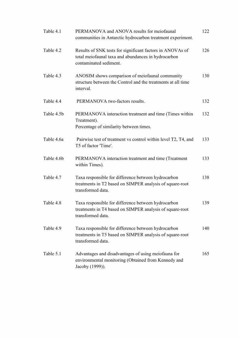
Table 4.1 PERMANOVA and ANOVA results for meiofaunal communities in Antarctic hydrocarbon treatment experiment.

122

Table 4.2 Results of SNK tests for significant factors in ANOVAs of total meiofaunal taxa and abundances in hydrocarbon contaminated sediment.

126

Table 4.3 ANOSIM shows comparison of meiofaunal community structure between the Control and the treatments at all time interval.

130

Table 4.4 PERMANOVA two-factors results.

132

Table 4.5b PERMANOVA interaction treatment and time (Times within Treatment). Percentage of similarity between times.

132

Table 4.6a Pairwise test of treatment vs control within level T2, T4, and T5 of factor 'Time'.

133

Table 4.6b PERMANOVA interaction treatment and time (Treatment within Times).

133

Table 4.7 Taxa responsible for difference between hydrocarbon treatments in T2 based on SIMPER analysis of square-root transformed data.

138


139


140

Table 5.1 Advantages and disadvantages of using meiofauna for environmental monitoring (Obtained from Kennedy and Jacoby (1999)).

165

1

1.0 GENERAL INTRODUCTION

The Antarctic continent is considered the most pristine place in the world due to its

remoteness and distance from inhabited regions of earth. This continent is far from

major human activities and sources of pollution. Nevertheless, this region is

susceptible to pollution caused by past and present human activities. There are more

than 60 research stations in Antarctica which are managed by at least 30 countries,

which are all signatory to the Antarctic Treaty. These research stations either operate

during summer or all year round. Having research stations all around the continent

may increase the risks of human pollution to the environment. Thus, countries

adhering to the Antarctic Treaty have accepted the Protocol on Environmental

Protection, often referred as the Madrid Protocol. These measures include establishing

monitoring programs for waste disposal, contamination by oil or other hazardous

toxic substances, construction and operation of stations, conduct of science programs,

recreational activities and activities affecting the purposes of designated protected

areas.

There are three permanent Antarctic stations which are maintained by the Australian

Antarctic Division. Casey Station (66o17’S, 110o32’E, East Antarctica) is the closest

of the permanent Australian Antarctic stations, situated 3430 km south of Hobart.

This station can accommodate up to 70 personnel over summer month and 20 over

winter. To assess the impact of this station, the Australian Antarctic Division (AAD)

has established an extensive environmental monitoring program in regards to human

activities and its impact on the environment.

2

1.1 Human impacts in Antarctica

The exploration and research of Antarctica have led to some significant although

often localized impact on the Antarctic environment (Aislabie et al., 2004). Several

impacts arise from human activities in Antarctica including oil spills, construction,

deposition of waste, introduction of alien species and disturbance to wildlife. Many of

these impacts have occurred on the small areas of ice-free ground, where the majority

of Antarctic scientific stations are located. Apart from environmental impacts by the

station, tourism may also contribute to human impacts in Antarctica. Ice free areas are

the focus of human activity and continue to attract scientists and increasing numbers

of tourists. This increase in the number of voyages to the continent is likely to

increase the risk of pollution by vessels.

While Antarctica has so far been relatively free from major petroleum spills, large

spills are likely to happen at sea in the future and these may spread onto nearby

shorelines, and involve fuel oils for ship and station use. The last catastrophe was

when Bahia Pariaso, which ran ashore near Palmer Station on the Antarctic

Peninsula, spilling about 600,000 litres of fuel (Lee and Page, 1997). Direct spillage

can also occur on land, at stations during delivery, storage and use of petroleum fuels.

In 1990, a spill of 91000 litres of SAB diesel fuel occurred from a fuel storage facility

at Casey Station (Deprez et al., 1999). Based on observation of fuel spills at Casey

Station, Antarctica, every 1 kg of fuel spilled creates between 100 to 1000 times that

amounts of contaminated soil by mass (Filler et al., 2008). Although, smaller volumes

are involved, petroleum spills have often occurred in environmentally sensitive areas

3

(Kerry, 1993). The main sources of hydrocarbon contamination in Antarctic coastal

marine environments are shipping operations near the scientific stations where fuel is

transported and refuelled, and also human activities such as vehicle use, fuel storage,

transfers and waste disposal.

Few studies on human impacts have been conducted on the marine environment of

Eastern Antarctica and most have been conducted in shallow waters (Stark et al.,

2003c, Stark, 2000, Thompson et al., 2003, Stark et al., 2004). Several studies have

been conducted in areas near Casey Station, investigating the contamination and

human impacts due to the station operations. Previous studies in the area have

focussed on how benthic microbial (Powell et al., 2005), diatom (Cunningham et al.,

2003) and infaunal communities (Thompson et al., 2007) responded to metal and

petroleum hydrocarbon pollution. Stark et al. (2003c) assessed the recruitment and

development of soft-sediment assemblages from hydrocarbon-contaminated marine

sediments, and found that there was a significantly reduced crustacean abundance in

these sediments (i.e., gammarid, ostracods, tanaids and copepods) in comparison to a

reference site. Stark et al (2003a) provided fundamental baseline information of

disturbed and undisturbed sites at Casey Station. This study was to determine the

appropriate scales and levels of spatial replication, the most suitable level of

taxonomic resolution and influence of data transformation in shallow marine (max 20

metres) infaunal assemblages at Casey. Variations in populations were found at

smallest scale, between replicates core and also at the level of location. Meanwhile,

the patterns of assemblage structure were found similar only at fine and medium

levels of taxonomic resolution. Stark et al (2003a) found that identification of

differences between control and impacted areas can be done at coarse levels (phyla)

4

of taxonomic resolution. This was supported the findings of other studies that

suggested analyses at higher taxonomic levels are useful to pollution monitoring

programs (Warwick, 1988, James et al., 1995). Correlations between spatial

distribution of soft sediment assemblages and environmental variables (heavy metals,

sediment grain size and total organic carbon) at Casey Station were done by Stark et

al. (2003b). Impacted locations (Wilkes, Brown Bay, Shannon Bay and Wharf) were

characterised by fewer taxa, lower diversity and lower species richness. Sparkes Bay,

one of the control locations in the study also had concentrations of cadmium and

nickel, low abundances, diversity and richness similar to the impacted locations.

Combination of toxicity and sediment anoxia caused by high TOC levels and fine

sediment contributed by large amounts of perennial kelp (Himantothalus sp.) were

found influencing assemblages at Sparkes Bay. In addition, study by Cunningham et

al. (2003)using benthic diatoms as pollution indicators have also been conducted at

Casey. The research focused on the effects of hydrocarbons on diatoms, where, results

showed that diatom community composition within Brown Bay at Casey was

significantly related to metal concentration (Cunningham et al., 2003). The responses

to metal contamination of the diatoms were species specific, with different species

showing different tolerance levels.

5

1.2 Marine Meiofauna

Meiofauna are one of the richest and most diverse aquatic communities in marine

benthic ecosystems. They occur in both freshwater and marine habitats, from

shorelines to the deep sea, and from tropics to polar regions. The marine meiofauna

contains numerous undescribed species and higher taxa.

The term meiofauna is derived from the Greek meio meaning “smaller” (Higgins and

Thiel, 1988). In this context, it refers to the fauna that are smaller than what has been

defined as the lower size limit for macrofauna, i.e. less than 500 µm. Meiofauna are

thus smaller than macrofauna but larger than microfauna (maximum size 32 μm). The

size range separates a discrete group of organisms whose morphology, physiology and

life history characteristics have evolved to exploit the interstitial matrix of marine soft

sediments (Kennedy and Jacoby, 1999). Meiofauna are found in all types of sediments

from softest muds to the coarsest gravels. Meiofauna can also occupy space several

centimetres above sediment habitats, including rooted vegetation, moss, macroalgae,

sea ice and various animal structures, e.g. coral crevices, worm tubes, echinoderm

spines (Higgins and Thiel, 1988). These communities play an important role in

sediment bioturbation and recycling of organic matter. They are also closely linked to

communities of primary producers as they are consumers of benthic microalgae (Hack

et al., 2007).

6

1.3 Components of the meiofaunal community

The meiofaunal community is comprised of 20 phyla (Table 1.1). Among these

phyla, Nematoda, Copepoda, Rotifera, Gastrotricha, Kinorincha and Tardigrada are

common in meiofaunal community. Although meiofauna consist of numerous groups,

in this study, two main dominant groups were examined. These are the Nematoda and

Copepoda. Within this community, Nematoda has shown a distinct dominance in

comparison to other groups (de Skowronski and Corbisier, 2002, De Leonardis et al.,

2008, Urban-Malinga et al., 2005, Vanreusel et al., 2000). For example, more than

60% of each community was made up of nematodes in Martel Inlet, King George

Island, Antarctica (de Skowronski and Corbisier, 2002).

1.3.1 Nematodes

Nematodes are abundant in marine sediments, dominating the coastal, and sub-littoral

and estuarine marine meiofauna, inhabiting even the deepest ocean trenches. They

move easily through mud and sand, but are poorly adapted to swimming so that they

do not occur in the plankton except as parasites or commensals of other animals.

Nematodes regularly dominate the meiofauna in the top 5 cm of sediment biotopes,

comprising more than 50% of the total meiofauna abundance.

7

Table 1.1: Currently, 20 phyla (bold) considered to be meiofaunal from the 34 recognized phyla of the Kingdom Animalia. Source : International Association of Meiobenthologists.

Phyla of the Kingdom Animalia

Phyla Free-living Symbiotic

Marine Freshwater Terrestrial Porifera Yes Yes No No Placozoa Endemic No No No Cnidaria Yes Yes No Yes Ctenophora Endemic No No No Platyhelminthes Yes Yes Yes Yes Orthonectida No No No Endemic (Marine) Rhombozoa No No No Endemic (Marine) Cycliophora No No No Endemic (Marine) Acanthocephala No No No Endemic Nemertea Yes Yes Yes Yes Nematomorpha No No No Endemic Gnathostomulida Endemic No No No Kinorhyncha Endemic No No No Loricifera Endemic No No No Nematoda Yes Yes Yes Yes Rotifera Yes Yes Yes Yes Gastrotricha Yes Yes No No Entoprocta Yes Yes No Yes Priapulida Endemic No No No Pogonophora Endemic No No No Echiura Endemic No No No Sipuncula Yes No No No Annelida Yes Yes Yes Yes Arthropoda (Copepoda, Halacaroidea, Ostracoda, Mystacocarida, Tantulocarida)

Yes Yes Yes Yes

Tardigrada Yes Yes Yes No Onychophora No No Endemic No Mollusca Yes Yes Yes Yes Phoronida Endemic No No No Bryozoa Yes Yes No No Brachiopoda Endemic No No No Echinodermata Endemic No No No Chaetognatha Endemic No No No Hemichordata Endemic No No No Chordata Yes Yes Yes Yes

8

Due to the lack of knowledge regarding many nematodes, their systematic are

contentious. Traditionally, the Class Nematoda is divided into two classes, the

Adenophorea and the Secernentea, and initial DNA sequence studies suggested the

existence of five clades: Dorylaimia, Enoplia, Spirurina, Tylenchina and Rhabditina

(De Ley and Blaxter, 2004).

The Nematode body is essentially a tube within a tube. The external wall consisting

externally of a cuticle layer and internally of a longitudinal muscle layer. The buccal

cavity and sensory organs such as amphids and setae are important for taxonomic

identification. Other important parts which are taxonomically useful are the nervous,

excretory and reproductive systems (Warwick and Clarke, 1998).

1.3.2 Copepods

In terms of meiofauna abundance, the Copepoda are second to the Nematoda in

sediments and probably exceed them in phytal habitats ( i.e: seagrass or algal beds).

There is considerable species diversity and copepods inhabit all available benthic

habitats in the sea, freshwater and inland saline waters, e.g. among mosses and

bromeliads, particularly in warm climatic regions (Wells, 1978). In sediments, they

tend to be found on or just beneath the surface of muds but also extend deep within

sands and gravels to the level of the permanent water table. In the sea they are

associated with sessile epibenthic macrofauna and are especially abundant and diverse

9

on macrophytes, where they form a large part of the phytal meiobenthos (Wells,

1978).

Each part of the copepod body is important for their taxonomic identification. The

body consists of three tagmata: the cephalosome, the metasome and the urosome. The

cephalosome consists of the head and first thoracic segment. The tergites and pleurites

of these segments are fused together to give a continuous head shield. The

cephalosome bears the head appendages antennule (first antenna), antenna (second

antenna), mandible, maxillule (first maxilla), maxilla (second maxilla) and the

maxilliped of the first thoracic segment. In most harpacticoids, the second thoracic

segment has become fused with the cephalosome to form a cephalothorax. The

metasome primitively consists of the thorax for the first segment, and bears the first

five pairs of “swimming legs”, or pereiopods (Wells, 1978).

The life cycle of copepod can determine their ecology. Their planktonic stages

includes six nauplius larval and five subadult copepodid stages during which there is a

progressive addition of prosome and ursome segments and development of their

appendages. During these stages, copepods are only found floating and swimming in

the water column.

The sexes can be distinguished by the fourth copepodid stage (Huys et al., 1996). All

species are sexually dimorphic but the only universal morphological difference is the

structure of the first two abdominal segments. In the female, these are fused into a

10

genital somite and the sixth pereiopod is reduced to one or two setae flanking the

single, median genital aperture. In the male the two segments remain separate and the

sixth pereiopod is far more elaborate than the female. Females are usually larger than

males. Other, almost universal sexual differences occur in the male antennule, which

usually is prehensile to a greater or lesser degree, and the fifth pereiopod, which

usually is smaller and less elaborate than the female. Sexual dimorphism may also be

apparent in pereiopods 1 to 4 but there is great variability in the form of such

differences between, and even within, families. There are currently ten groups of

copepods. Three main groups, Calanoida, Cyclopoida, and Harpactacoida are free-

living and most likely to be encountered. The Calanoida and Cyclopoida are

primarily planktonic. The Harpactacoida are primarily benthic, as evidenced by their

vermiform (worm-shaped) bodies. At present the Order Harpacticoid copepods

contains about 2757 species distributed among 346 genera in 33 families.

Harpacticoid copepods range in size from 0.2 mm to 2.5 mm (Giere, 1993) and thus

can all be classed as meiofauna.

1.4 Patterns of meiofauna distribution

Some macrofauna are a part of the meiofauna only during their juvenile stages, but

many taxa contain species that are meiofauna throughout their life cycles. This

permanent meiofauna includes the Mystacocarida and many representatives of

Rotifera, Nematoda, Polychaeta, Copepoda, Ostracoda and Turbellaria. Many studies

have shown that the distribution patterns of meiofauna are affected by factors such as

the sediment type, depth and food availability (de Skowronski and Corbisier, 2002,

11

Veit-Köhler et al., 2008, Gutzmann et al., 2004). A high abundance of nematodes was

found to be positively correlated with the presence of a high abundance of

cyanobacteria (Doulgeraki et al., 2006). A higher percentage of meiofauna biomass is

recorded from brackish water,, intertidal beaches and from the deep sea, where

meiofauna and macrofauna biomass are of the same magnitude (Gerlach, 1971).

There are approximately 106 m-2 meiofaunal organisms in almost every natural

(uncontaminated) estuarine sediment worldwide and a dry weight standing crop

biomass of 0.75 – 2.0 gm-2 (Coull and Bell, 1979).

Certain taxa are restricted to particular sediment types. Sediments where the median

particle diameter is below 125 μm tend to be dominated by burrowing meiofauna

(Coull, 1988). The interstitial groups, for example the Gastrotrichia and Tardigrada,

are typically excluded from muddy substrates where the interstitial lacunae (cavity)

are closed. The sand fauna tends to be slender as it must manoeuvre through the

narrow interstitial openings, whereas the mud fauna is not restricted to a particular

morphology but is generally larger (Coull and Bell, 1979). In general, sediment grain

size is a primary factor affecting the abundance and species composition of

meiofaunal organisms. For example the genus Astomonema, Terschellingia, Theristus,

Sabatieria and Dorylaimopsis were found to be highly dominant in muddy sediment

and to have a low abundance in sands (De Leonardis et al., 2008).

Benthic nematodes are among the primary consumers of bacterial. Moens et al (1999)

concluded that selective recruitment to food spots may be a major factor driving the

heterogenous field distribution of bacterivorous nematodes. Gray and Johson (1970)

12

documented that bacterial films on sand grains differently attract meiofaunal

organisms. Moens et al (1999) demonstrates a highly species specific marine

nematode (Monhystera sp.) preference to Gram-negative bacterial. However,

Warwick (1981) found that the occurrence of a species in a specific biotope is not

only determined by its feeding behaviour, but also factors such as reproductive

capacity, tolerance to environmental conditions, competition and predation, which all

play roles in the survival strategy of nematode species (Bouwman, 1984). This is

because, same taxa have the ability to switch their diet when a specific food items is

limited (Moens and Vincx, 2009) or when the quality of organic matter available to

the deposit and epistratum-feeders changes with season. In the study by Da Rocha et

al. (2006), they found that presence of nematode not only influenced by food

availability but also the complexity and type of habitat. For example, they suggested

that Halalaimus sp. showed the specificity based on habitat type as this species was

found almost restricted (94%) to in habitat dominated by Hypnea musciformis and

Padina gymnospora.

In almost all meiofauna studies, the majority of the fauna has been found in the upper

2 cm of sediment. Vertical zonation is controlled by the depth of the Redox Potential

Discontinuity (RPD) level, i.e. the boundary between aerobic and anaerobic

sediments. The primary factor responsible for vertical gradients in the RPD is oxygen

(McLachlan (1978), which determines the redox potential as well as the oxidation

state of sulphur and various nutrients. When redox potentials are low, meiofauna

densities greatly decrease.

13

Harpacticoid copepods are typically the most sensitive meiofauna taxon to decreased

oxygen, and are usually restricted to oxic sediments (Wieser et al., 1974). Some

meiofauna appear to be capable of tolerating low or no oxygen conditions and thus

penetrate sediments below the RPD (Reise and Ax, 1979). There is however, a debate

over how these animals adjust to reduced O2 levels (Schiemer et al., 1990) and

whether the occupied habitats below the RPD are truly anoxic (Boaden, 1980). In

mud and sediments heavy in detritus, meiofauna are often restricted to the upper few

mm or cm of oxidized sediments (Coull and Bell, 1979). Most of the research on

vertical patterns of meiofauna vertical distribution has been conducted in sandy

substrata (Gheskiere et al., 2004, Gheskiere et al., 2005, Rodri´guez et al., 2003,

Nicholas and Hodda, 1999) and deep sea (Vanreusel et al., 1995, Steyaert et al.,

2003). In sands the meiofauna can be distributed to the depth of the RPD, which on

high energy beaches can be 50 cm or more deep (Higgins and Thiel, 1988). Oxygen

content is the ultimate factor controlling vertical distribution of meiofauna in beaches

(McLachlan, 1978).

Meiofauna are also known to be sensitive to low pore water content (Jansson, 1968).

As sand dries at low tide, the fauna face desiccation stress despite the oxygen content.

McLachlan et al. (1977) found that meiofauna migrated downwards on an ebbing tide

and upwards on a flooding tide. Vertical migration is typically less in winter than in

summer and this appears to be related to lower winter temperatures and therefore less

desiccation at low tide than in the summer. Furthermore, vertical migration is reduced

at night, probably in response to cooler night temperatures at low tide and again, less

desiccation. Thus, the migrations are not entirely dependent on the tides since

desiccation varies seasonally and diurnally.

14

It is well known that environmental disturbance affect the distribution of organisms in

a given ecosystem. The abundance and distribution of meiofaunal communities are

also influence by natural disturbance such as bioturbation (Sellanes and Neira, 2006),

storms (Peck et al., 1999), tidal effects (Gheskiere et al., 2006) and iceberg scouring

(Gutt and Piepenburg, 2003, Gutt et al., 1996, Lee et al., 2001, Gerdes et al., 2003,

Peck et al., 1999). Among the natural disturbance, influence by icebergs scouring is

the important in the polar region. Whereby, icebergs affect soft substrata in three main

ways. Firstly, they plough the seabed that forces surface layers away from the point of

contact; second, they crush it, whereby icebergs rock backwards and forwards

crushing underlying organisms and seabed; and finally, water flowing around icebergs

either caused by movements of the berg, natural oceanic currents, or salinity induced

water actions can resuspend and transport sediment (Reimnitz et al., 1977). These

changes will subsequently alter the habitats, sediment properties and food availability.

In any disturbance there is an immediate change in the abundance and diversity of

meiofauna but there is subsequent recovery. When an area occupied by a set of

species is disturbed, re-colonization and succession will occur with a new set of

species (Mani et al., 2008). For example, Raes et al (2010) noted that nematodes

appear to be strongly influenced by the sudden removal of ice-cover in the Antarctic

Larsen ice shelf area. Raes et al (2010) indicate that pre-collapse, sub-ice

communities were impoverished and characterized by low densities, low diversity and

high dominance of a few taxa. However, an increase in food supply after ice-cover

removal provoked a fast, local response of the nematode assemblages to

recolonization. The collapse of the ice shelves showed a positive effect on the shelf

nematode fauna in the area, both in terms of abundance and diversity. In a study by

Kotwicki et al (2004), they found that glacial runoff (freshwater input) and enhanced

15

sedimentation rates at Kongsfjorden, Spitsbergen reduces the number of individuals in

the meiofaunal community.

Apart from recolonization of species as a response to disturbance, these communities

are also able to adapt to the changing environment. For example, Gheskiere et al

(2005) suggested that nematodes in dynamic environments usually exhibit

morphological adaptations (such as body ornamentations which provide an

anchorage) to high turbulence and shifting sediments. Seasonal changes may also alter

the abundance and biomass of the community. In a study by Rudnick et al (1985),

they observed that highest abundances and biomass occurs in May and June, while

lowest values were in late summer and autumn. In springtime increases of meiofauna

were observed. They concluded that microalgae detritus accumulated in the sediment

during winter and early spring, and the meiofaunal responded to this store of food

when temperatures rose rapidly in the late spring.

1.5 Past research on meiofauna in Antarctica

Early studies of marine nematodes from Antarctic waters, were based on collections

made by various national expeditions between 1882 and 1931 (Platt and Warwick,

1983, De Broyer et al., 2007). In the Atlantic sector of the Antarctic Ocean, material

from shallow sublittoral areas of South Georgia and the west coast of the Antarctic

Peninsula were obtained from diving and grab-sampling in deeper waters off South

Georgia and in the Weddell Sea. It is suggested that detailed studies of nematode

16

communities could provide a valuable method of addressing some of the classical

aspects of Antarctic biology.

Scientific publications on Antarctic nematodes are scarce. The first nematode to be

described from Antarctic waters was Deontostoma antarcticum, collected at South

Georgia during the German International Polar-Year Expedition (1882-1883).

Descriptions of meiofauna collected by various national expeditions include the

following. Initially, 13 nematodes were collected and described by Larsen's Ross Sea

Expedition (1929-1930) from Macquarie Island and in the Ross Sea (Allgen, 1930).

Other report of nematodes are from the Antarctic Peninsula (Inglis, 1958). Linstow

(1907) also provided the first description of a nematode from the East Antarctic

(Leptosomatum australe from the Ross Sea). Later, Cobb (1914) described 25 new

species collected in the Ross Sea by Shackleton's Expedition (1907-1909).

Epsilonematidae and Desmoscolecida, collected by the German Antarctic Expedition,

The Gauss Expedition (1901-1903), were described by Steiner (1931b, 1931a) and

Timm (1970) respectively. Mawson's two Antarctic expeditions (1911-1914, 1929-

1931) provided material which resulted in the valuable contributions of Cobb (1930)

and Mawson (1958a, 1958b). Further descriptions of Enoplida from Kerguelen Island

were made by Schuurmans-Stekhoven and Mawson (1955) and Platonova (1958).

Studies involving nematodes also have been reported from the Ross Sea (Hope, 1974,

Timm and Viglierohio, 1970), Kerguelen Island (Arnaud, 1974, de Bovee and Soyer,

1975) and Weddell Sea (Vanhove et al., 1999, Herman and Dahms, 1992, Vermeeren

et al., 2004, De Mesel et al., 2006, Fonseca et al., 2006)

17

A detailed history of copepods recorded from Antarctica by several expeditions was

written by Golemansky and Chipev, (1999) in their book entitled “Bulgarian

Antarctic Research. Life Sciences”. In this book, it was stated that the first records of

harpacticoid copepods from the Antarctic were given by Giesbrecht (1902), who

described the copepods collected during Belgica Expedition (1897-1899). It were then

followed by Brady (1910), who worked on the material of the German Southpolar

Expedition (1901-1903) and discovered Harpacticus simplex, Mesochra nana,

Laophonte gracilipes and Amphiascus minutes during the expedition. Later, Lang

(1936) described a new species, Amphiascus gracilis, from the same material.

Harpacticoid copepods have also been collected by the British Antarctic Expedition

(1902-1904) and the French Antarctic Expedition (1903-1905). The materials of the

French Expedition were identified by Quidor (1920) who reported three harpacticoid

species of the genus Porcellidium. Golemansky and Chipev, (1999) discussed the

species composition of harpacticoids collected by the Australian Antarctic Expedition

(1911-1914) that included seven harpacticoid species from the region of Kerguelen

and St. Paul Island and were published by Monard & Dollfus (1932), Lang (1934) and

Brady (1918).

There have been many studies reporting the distribution of harpacticoid copepods in

Antarctica, such as; the Weddell Sea (Schnack-Schiel et al., 2001, Günther et al.,

1999, Dahms et al., 1990, Herman and Dahms, 1992, Vanhove et al., 1995, Dahms,

1989), Ross Sea (Bradford and Wells, 1983, Gambi et al., 2004), Amery Ice Shelf

(Swadling et al., 2000), Vestfold Hills (Swadling, 2001), Langhovde (Kudoh et al,

2008), Syowa Station (Hoshiai et al., 1996), King George Island (Veit-Kohler and

Fuentes, 2007), Kerguelen (Huys and Conroy-Dalton, 2006).

18

Studies carried out in the Weddell Sea confirmed the presence of a relationship

between meiofauna distribution and food indicators (Lee et al., 2001) but also

reported high meiofaunal densities compared to similar deep environments at

temperate latitudes (Herman and Dahms, 1992). Studies have shown that the

meiofauna community shows a pattern of decreasing densities with increasing water

depth (Gutzmann et al., 2004, De Leonardis et al., 2008, Vanhove et al., 1995), which

is related to a reduction in organic matter and food availability. Although meiofauna

in polar regions show a large spatial variability (Vanhove et al., 2000) the parameters

which control meiofauna distribution and community structure are still unclear.

A study by Fabiano and Danovaro (1999) on meiofauna distribution in the Ross Sea

described different trophic and sediment characteristics and indicated that at macro-

scales (kilometres) meiofaunal communities are dependent on particulate organic

matter fluxes. At micro-scales (centimetres) a very low variation in meiofauna density

contrasted with large meso-scale (metres) variability, which was related to the

concentration of the main food indicators such as phytopigments, proteins,

carbohydrates and lipids.

1.6 Meiofauna as an indicator species

Marine benthic organisms and communities have commonly been used as a focus of

monitoring programs(Tin et al., 2008) and in research into the effects of human

activities in the marine environment (Platt and Warwick, 1983). Environmental stress,

19

such as pollution, is considered to decrease marine benthic organism species diversity

i.e. total number of species or taxonomic groups (Warwick and Clarke, 1995, Clarke

and Warwick, 1994). They are used in monitoring programs due to their relative lack

of mobility and their trophic position (Kennedy and Jacoby, 1999, Gomez Gesteira et

al., 2003). Firstly, these sedentary organisms are less mobile and this will reduce their

chance of avoiding potentially harmful conditions (Sutherland et al., 2007) and

secondly, nearshore benthic organisms are often closely coupled with pelagic food

webs, constituting a link for the transport of contaminants to higher trophic levels

(Coull, 1990).

Changes in benthic faunal communities have been used as indicators of contamination

and pollution in marine ecosystems (Simboura and Zenetos, 2002, Kennedy and

Jacoby, 1999, Bustos-Baez and Frid, 2003, Kennish, 1998). Meiofaunal communities

have been considered better indicators of pollution and human impacts in the marine

benthic environments than macrofauna communities as they have a shorter life cycle

and are more sensitive to environmental changes. As a direct benthic developer,

meiofauna stay in the sediment throughout their life cycle. Furthermore, as they are

smaller and have limited mobility they are ideal organisms as pollution indicators. As

meiofauna are also in constant contact with water in the sand they are thought to be

more reliable indicators of pollution than bivalves, which siphon water from the

overlying water column. Meiofauna comprise a basal component of the food web and

disturbing them could have unforeseeable trophic consequences. Altered species

composition could significantly influence interactions between nematodes and

interactions among major benthic taxa (Mahmoudi et al., 2005, Austen et al., 1994,

Austen and McEvoy, 1997). In addition, many juvenile fish and crustaceans prey on

20

meiofauna, particularly nematodes and copepods (Coull, 1990). Responses of free

living nematodes to diesel contamination (elimination of some species, increase or

decrease of some others) could lead to food limitation for juvenile fish and

crustaceans which could ultimately alter entire communities and ecosystems

(Warwick and Clarke, 1998).

Meiofaunal assemblages are ideal for experimentation as they are small, abundant,

have a short life cycle, are easily maintained, and are sediment bound throughout their

life history (Higgins and Thiel, 1988). The meiofauna are the most abundant

metazoan component of marine organisms. Total meiofauna densities may exceed

1.29 x 107 individuals per square meter of sediment surface (Warwick et al., 1979)

while densities of individual species may reach 5.7 x 106 m2 (Hicks, 1988). Their

close association with sediment means that changes in interstitial chemistry quickly

feeds through to changes in meiofauna abundances and diversity.

Meiofaunal assemblages and, in particular nematodes have been increasingly utilized

as indicators of organic disturbance because of their ubiquity, high densities and high

taxonomic diversity (Mirto et al., 2002). Meiofauna possess a number of advantages

over macrofauna in their suitability for data collection. The organisms are sufficiently

small and numerous to allow small volume sediment cores to contain statistically

adequate counts of total fauna. This means that many replicate samples can be

collected by SCUBA divers without the need for a field-biased processing stage.

However, Kennedy and Jacoby (1999) suggested that there were also some

disadvantages in using meiofauna as pollution indicators. Meiofauna are very small,

21

thus, identifying these organisms is time consuming. Thus, due to lack of research and

study, the availability of the identification keys is limited. Kennedy and Jacoby (1999)

also concluded that the meiofauna have a high level of spatial and temporal variability

in their distribution. The abundances of meiofauna are also effected by environmental

factors such as salinity (Soetaert et al., 1995), sediment type (Veit-Köhler et al., 2008)

and wave effects (Rodri´guez et al., 2003) and these factors will also affect the

interpretation of the results.

Parker (1975) and Raffaelli and Mason (1981) have proposed using the ratio of

nematodes to copepods (N/C ratio) as a monitor of pollution or sediment changes that

eliminates the need for detailed, time consuming taxa identification. While, this idea

is very attractive, it has generated considerable controversy (Warwick, 1981,

Lambshead, 1984, Raffaelli and Mason, 1981, Platt et al., 1984, Coull et al., 1981)

and it has not been proven to be an accurate predictor of environmental change.

While, the technique is simple because no taxonomic experts need be sought, further

research is needed to determine the universality of the N/C ratio as a measure of

environmental perturbation. Because of rather difficult taxonomy of meiofauna; many

perturbation studies prefer not to include them.

Previous studies have shown that meiofauna have similar responses to macrofauna to

human disturbances of aquatic environments (Coull and Chandler, 1992, Peterson et

al., 1996, Schratzberger and Jennings, 2002) and are very sensitive to different

sources of organic contamination (Mirto et al., 2002). Peterson et al. (1996) argued

that macrofaunal and meiofaunal communities display repeatable patterns of response

22

to environmental stressors, which are generally detectable at high taxonomic levels

(even phyla). Hence, echinoderms and crustaceans, especially amphipods and some

harpacticoid copepods, are highly sensitive to toxic chemicals in their environment

and these groups typically show large declines in abundance due to sediment toxicity.

By comparison, nematodes, polychaetes, and oligochaetes are not especially sensitive

to toxins. These groups tend to include species with opportunistic life histories and

less susceptible feeding types (especially non-selective deposit feeders) that render

them capable of utilizing organic materials associated with organic enrichment.

These taxa typically show substantial increases with organic pollution where oxygen

depletion is not a factor (Peterson et al., 1996). While, nematodes are highly tolerant

to stressed environmental conditions, copepods are sensitive to biodeposition (Mirto

et al., 2002). This suggests that organic enrichment of sediments will alter the

abundance and community structure of meiofaunal assemblages.

23

1.7 Research Objectives

This study had three main aims: A) To investigate meiofaunal communities in the

Casey region and determine their composition, distribution and abundance and

patterns of spatial variation; B) to determine whether there were any correlations

between community patterns and environmental variation, including potentially

impacted areas; C) to assess the effects of sediment hydrocarbon contamination on

Antarctic meiofaunal communities. In order to achieve this, the study was divided into

three parts (Figure 1.1). All free-living nematodes and harpacticoid copepods were

identified.

Figure 1.1: Structure of the research.

The ecology of Antarctic meiofaunal communities from Casey Station: spatial variation and human

impacts

Spatial survey

Hydrocarbon experiment

Correlations between spatial patterns and environmental data

ENVIRONMENTAL DATA

24

A. Spatial Survey

A survey of meiofaunal communities was undertaken to determine the spatial

variation, abundance and biodiversity of meiofauna. A spatially nested sampling

design was used in this survey. The design allows comparisons of variability at

several scales: at ~10 m among plots within sites, at ~100 m among sites within

locations and between the locations. O’Brien Bay (O’Brien Bay 1 and O’Brien Bay 5)

and McGrady were considered as control locations. Surveys were also undertaken at

two locations impacted by abandoned waste disposal sites. The disturbed locations are

Brown Bay (Brown Bay Inner and Brown Bay Middle) and Wilkes.

The first objective of this component was to investigate and describe the spatial

patterns of community composition and abundance by looking at the natural variation

at different scales, from meters to kilometres. The second objective was to compare

the control locations and disturbed locations (waste disposal sites).

The hypothesis that was being tested in this spatial survey study was there will be

differences in meiofaunal communities between locations and within locations.

25

B. Correlations between spatial patterns and environmental data

The aim of this component is to examine relationships between meiofaunal

communities and environmental patterns. The main environmental variables used are

sediment properties such as grain size, organic carbon and metals in sediments.

Multivariate biological and environmental datasets will be examined to determine

whether there any correlations between patterns of community composition and

environmental variables. Such relationships will suggest causal relationships between

environmental variables and differences in meiofaunal community structure.

C. Hydrocarbon Experiment

The objective of this study is to experimentally investigate the responses of free-living

nematode and harpacticoid copepod communities to hydrocarbon pollution. Benthic

invertebrates may be continuously exposed to Polycyclic Aromatic Hydrocarbons

(PAHs) in contaminated areas since PAHs are relatively insoluble in water, absorb

strongly to particulate matter and accumulate in bottom sediments. Furthermore, they

are a high risk and common pollutant. Thus, the aim is to demonstrate a causal link

between presence of hydrocarbon pollution and environmental impacts. The

experiment was setup to monitor their response change through time up to five years

(260 weeks). There are five period of sampling (T1, T2, T3, T4 and T5) but in this

study only T2 (54 weeks), T4 (102 weeks) and T5 (260 weeks) were monitored.

26

The hypotheses being tested here are:

1. There will be differences between in meiofauna communities in control and

oiled treated experiments.

2. The effects on meiofaunal communities will be different among the different

oil treatments used in the experiments

3. Duration of exposure to oil treatment will affect meiofaunal abundance and

community composition.

27

2.0 SPATIAL VARIABILITY OF MEIOFAUNAL COMMUNITIES AT

CASEY STATION

2.1 Introduction

The meiofauna is defined as animals passing through a 1.0 mm sieve but retained on a

32 µm mesh. However the distribution of meiofauna is strongly related to the amount

of utilizable organic matter in the sediment (Fabiano and Danovaro, 1999), which is

controlled by sedimentation and organic degradation rates (Doulgeraki et al., 2006).

Meiofauna can stimulate microbial activity in the sediment (Tenore et al., 1977), they

are food for the macrofaunal communities (Gee, 1989) and they can also be a

potential bioindicator of environmental impacts.

De Leonardis et al. (2008) suggested that the abundance and distribution of meiofauna

was related to water depth, whereby shallower sites having a greater abundance and

diversity and deeper sites having lower densities and a lower number of taxa. Similar

results were also found by Gutzmann et al. (2004), where, the abundance of

nematodes and copepods decreased with increasing water depth. Doulgeraki et al.

(2006) suggesting that bottom currents, sediment particle size and pH were the most

important factors explaining spatial differences in meiofaunal. In addition, De Troch

et al. (2001) found that at South of Mombasa Island, Tanzania the variation within

meiofauna assemblage was linked to the specific habitat requirements whereby certain

genus of meiofauna very only found on certain seagrass species. They concluded that

meiofauna was structured by environmental conditions as selected and partly created

by the seagrass species. The habitat selected by the seagrass species, in view of its

28

role in the succession, in terms of grain size, organic matter and pigments determines

the associated meiofauna.

Coastal benthic habitats are among the most productive of marine environments

(Barnard, 1998, Levinton, 1995, Borum and Sand-Jensen, 1996, Suchanek, 1994).

They typically receive a rich nutrient supply, which is influenced by both terrestrial

nutrient sources and coastal phytoplankton production. In Antarctica, however,

terrestrial nutrient supply is extremely limited or almost entirely absent as there are no

rivers and little terrestrial primary production. The oceanic waters surrounding the

Antarctic continent are characterised by high nutrients levels, which often become

seasonally low during the summer, but rarely to levels that could be considered

limiting to the growth of phytoplankton. In Antarctic coastal areas nutrients are

relatively high throughout the year and are only briefly lowered during summer

(McMinn and Hodgson, 1993, McMinn et al., 1995).

The understanding of the ecology of meiofauna has increased in the last 20 years.

However, most quantitative information is limited to the Atlantic (Vincx et al., 1994.,

Vanreusel et al., 2009, Sebastian et al., 2007, Van Gaever et al., 2004, Vanreusel et

al., 1995), Pacific and Indian Oceans (Grove et al., 2006, Vincx et al., 1994,

Shirayama and Kojima, 1994, Gambi et al., 2003) and to the Mediterranean Sea

(Soyer, 1985, Soetaert and Heip, 1995, Danovaro et al., 1995, Pusceddu et al., 2009,

De Leonardis et al., 2008, Doulgeraki et al., 2006, Vezzulli et al., 2003, Mirto et al.,

2002, Moreno et al., 2009). Other studies of meiofauna include temperate coastal

shores (Rudnick et al., 1985, Veit-Köhler et al., 2008), tropical seagrass bed (De

Troch et al., 2001), subtropical shores (Grove et al., 2006) and mangrove ecosystems

29

(Armenteros et al., 2006), where they are the numerically dominant (Armenteros et

al., 2006).

As far as meiofauna is concerned, very scarce information is available from polar

regions. To date, only few investigations have been carried out in northern boreal

waters (Bick and Arlt, 2005, Pfannkuche and Thiel, 1987), for example, the Laptev

Sea (Werner and Martinez Arbizu, 1999, Vanaverbeke et al., 1997). As for Antarctica,

in the Weddell Sea (Lee et al., 2001a, Sebastian et al., 2007, Herman and Dahms,

1992, Vanhove et al., 1999, Schnack-Schiel et al., 2001, Vermeeren et al., 2004,

Schnack-Schiel et al., 2008) and in Ross Sea (Fabiano and Danovaro, 1999)

The structure, composition, and diversity of the Antarctic meiofauna are poorly

understood, particularly in East Antarctica. There are only a few studies on

meiofaunal communities in the eastern part of Antarctica (Swadling et al., 2000, Kito

et al., 1996, Swadling, 2001). Kito et al. (1996) described a new species of nematode,

Eudorylaimus andrassy, 1959 which was found among green algae near the Russian

Station, the Molodezhnaya. Research in Antarctica has included distribution

(Gutzmann et al., 2004, Vanhove et al., 2004, Doulgeraki et al., 2006) spatial and

temporal variation (Armenteros et al., 2006), assessment of pollution (Somerfield et

al., 1994), colonization (Veit-Köhler et al., 2008, Urban-Malinga et al., 2005) and

relationships to environmental factors (Vanhove et al., 1995).

The distribution of meiofauna in polar regions also varies with environmental factors.

Studies by de Skowronski and Corbisier (de Skowronski and Corbisier, 2002) suggest

that the meiofaunal density in the shallow coastal zone in King George Island,

30

Antarctica is very high compared to coastal studies in other regions. Skowronski &

Corbisier (2002) concluded that most meiofaunal studies in polar regions showed a

pronounced dominance of nematodes, followed by copepods. Their study of King

George Island (Antarctic Peninsula) found that nematodes comprised more than 60%

of the meiofauna, while, Fabiano and Danovaro (1999) found that nematodes

comprised 53% -80% of the meiofauna at Ross Sea, Antarctica. The explanation for

this dominance is thought to be because nematodes possess an incredible ability to

adapt to the most varied environmental conditions (Lee and Van de Velde, 1999,

Vanreusel, 1990, Vanreusel, 1991, Vanreusel et al., 1997). Fabiano and Danovaro

(1999) noted that meiofauna in two sampling location in Ross Sea, Antarctica

whereby distance between sampling corers were about 300-800 metres, a large spatial

variability on a scale of a few hundred meters were observed, but the parameters

controlling their distribution and community structure were however unclear. In a

study conducted by Gobin and Warwick (2006), they found that generally nematode

abundances were lowest in polar regions (Signy Island), greater in temperate (South

west England and New Zealand) and highest in tropical regions (Trinidad and

Tobago). Their study also suggested that there are some similar species found in both

tropical and temperate areas.

The shallow coastal benthic habitat in Casey Station consists of small areas of soft-

sediment which are interspersed between patches of rocky habitat. The shallow

habitats in areas that are covered by annual sea ice for much of the year are occupied

by various communities dominated by sponges, ascidians, tubeworms and other

invertebrates (Stark et al., 2003b). In areas with longer periods of open water and less

sea ice cover, benthic communities are dominated by macroalgae. The benthic

31

community at Casey Station has been studied extensively, including research on the

benthic diatom communities (Cunningham et al., 2005, McMinn et al., 2004) and the

effect of human impacts on benthic communities (Stark et al., 2003a, Stark, 2000,

Cunningham et al., 2003b, Powell et al., 2005, Stark et al., 2005).

The major aims of this study are a) to determine the spatial variability of the

meiofaunal communities at three different scales: Locations (up to several kms); Sites

within locations (~100 m); Plots within sites (~10 m) and b) investigate potential

human impacts on meiofaunal communities, comparing three control and three

contaminated locations near Casey Station. This research can be also used as a

baseline for future studies and provide an overview of the meiofaunal assemblage

inhabiting the shallow coastal water at Casey.

32

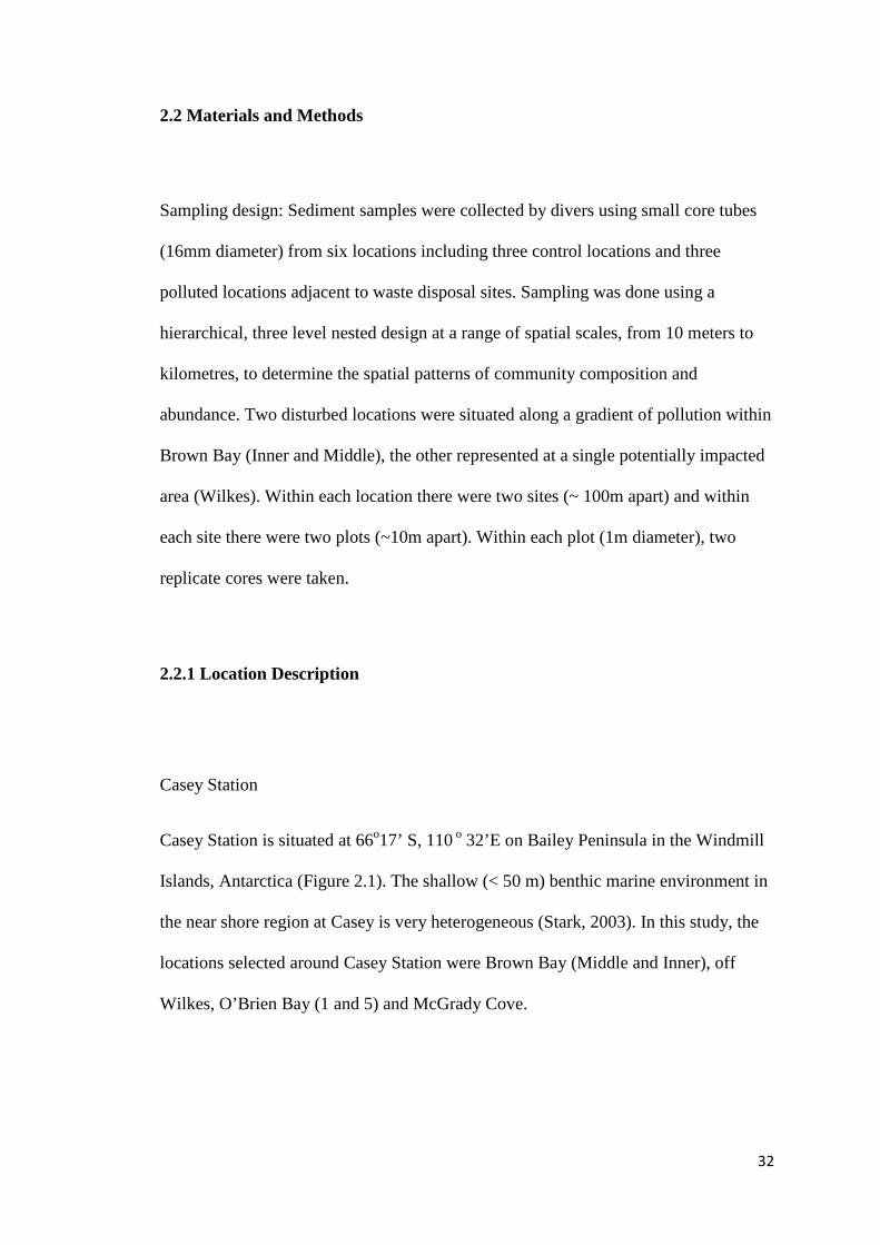
2.2 Materials and Methods

Sampling design: Sediment samples were collected by divers using small core tubes

(16mm diameter) from six locations including three control locations and three

polluted locations adjacent to waste disposal sites. Sampling was done using a

hierarchical, three level nested design at a range of spatial scales, from 10 meters to

kilometres, to determine the spatial patterns of community composition and

abundance. Two disturbed locations were situated along a gradient of pollution within

Brown Bay (Inner and Middle), the other represented at a single potentially impacted

area (Wilkes). Within each location there were two sites (~ 100m apart) and within

each site there were two plots (~10m apart). Within each plot (1m diameter), two

replicate cores were taken.

2.2.1 Location Description

Casey Station

Casey Station is situated at 66o17’ S, 110 o 32’E on Bailey Peninsula in the Windmill

Islands, Antarctica (Figure 2.1). The shallow (< 50 m) benthic marine environment in

the near shore region at Casey is very heterogeneous (Stark, 2003). In this study, the

locations selected around Casey Station were Brown Bay (Middle and Inner), off

Wilkes, O’Brien Bay (1 and 5) and McGrady Cove.

33

Brown Bay

Brown Bay is a small embayment at the southern end of Newcomb Bay with a

maximum depth of approximately 20 m and with rocky sides grading to a muddy

bottom (Cunningham et al., 2003b). Brown Bay is typically ice free for 1 to 2 months

in a year, usually in January and February. It is situated adjacent to the abandoned

Casey waste dump, which was on the foreshore of the bay, at the base of Thala Valley

(Stark et al., 2003b). Samples were taken from 2 locations within Brown Bay: Brown

Bay Inner was 30 m from the waste dump directly in front of the point where summer

melt water from the valley enters the bay (Stark et al., 2006) and at a water depth of 7

m. Brown Bay Middle was 150 m from the waste dump and ranged from 12 to 15 m

in depth.

Wilkes

The first Australian station in the area, Wilkes was built by the USA in 1957 on Clark

Peninsula on the shore of Newcomb Bay but was abandoned in 1969 (Cunningham et

al., 2005). The Wilkes waste dump site is on the foreshore of a small embayment on

the northern side of Newcomb Bay. It has a gently sloping bottom and the sampling

site was in approximately 15 m water. The marine benthic habitat consists of coarse

sandy sediments and areas of exposed rock covered with microalgae in summer.

Samples were collected from approximately 50 m directly in front of the waste dump.

34

O’Brien Bay

O’Brien is a large bay situated several kilometres south of Casey station. This site is

clean and unlikely to be contaminated by human activities. Therefore, the area was

selected as a reference location. The benthic habitat consists of rocky bottoms,

boulders, cobbles and gravel overlain by small patches of sediment (Stark et al.,

2003a). Samples were taken in approximately 15–20 m of water.

35

Figure 2.1: Map shows the location of spatial survey study

36

2.2.2 Meiofauna preparation and identification

The preserved sediment was initially sieved through a 500 µm sieve to remove the

coarser fraction. Meiofauna taxa were extracted from muddy sediment through a

modified gravity gradient centrifugation technique (Heip et al., 1985, Pfannkuche et

al., 1988) using Ludox. Ludox HS40 and Ludox AS both have a density greater than

the density of meiofauna, i.e. 1.08 for nematodes, but similar for all hard-bodied

meiofauna (Witthoft-Muhlmann et al., 2005). Ludox is a silicasol (a colloidal solution

of Si02) which causes no plasmolysis. Ludox HS40 is toxic and so could only be used

for preserved material. Ludox AS is not toxic and could be used when living

meiofauna had to be separated from sediments. For both types of Ludox, a 50%

solution in distilled water is used (density of 1.15). Samples were rinsed thoroughly

over a sieve of 32 µm with tap water to prevent flocculation of Ludox,.

The samples were transferred from the sieve to a large centrifuge tube. Ludox solution

(60% Ludox and 40% water; density = 1.18) was added to tube until the level of

mixture was balanced for centrifuging. The sample was then centrifuged at 2800 rpm

for 10 min. The supernatant was decanted and collected, and the remaining sediment

pellet was resuspended. This process was repeated three times. All supernatants were

filtered through a 100 µm sieve, followed by a 32 µm sieve. The supernatant was

finally rinsed through a 32 µm sieve with tap water to avoid the reaction between the

Ludox and formalin which forms a white gel which is difficult to remove. After the

extraction, 4% formaldehyde was added to the treated sample. The organisms retained

on the 32 µm sieve were fixed in 4% formaldehyde. The sample was stained with 1%

of Rose Bengal to facilitate counting.

37

All animals retained on the 32 µm sieve were counted and sorted into major taxa. The

major taxa (Nematoda and Copepoda) were counted using a dissecting microscope at

25X magnification (Zeiss Stemi 2000; Zeiss Inc., Germany). Per sample, 200

nematodes (or all nematodes when density less than 200 individuals.) were picked out

at random and mounted on slides in glycerine after a slow evaporation procedure

(modified after Riemann, 1988). For identification to genus level Platt and Warwick

(1983, 1988) and NeMys online identification (Steyaert et al., 2005) were mostly

used. All copepods were picked out and mounted on slides in glycerine without

evaporation for identification to family level using THAO: Taxonomische

Harpacticoida Archiv Oldenburg 2005 and Bodin (1997). The identification of

nematodes and copepods was done using 1000 times magnification.

2.2.3 Statistical methods

Univariate analysis of variance (ANOVA) was used to analyse meiofaunal

abundances in sediments. Analysis was done using the program GMAV5 (Underwood

and Chapman, 1998). A hierarchical spatially nested structure was used within the

asymmetrical analysis and the separate ANOVA from which it was constructed. The

sums of squares for the asymmetrical analyses were taken from three factor ANOVA

(location, site nested within location, and plot nested within site). Cochran’s test was

used to test for homogeneity of variances in ANOVAs. If variances were

heterogeneous, data were transformed (Snedecor and Cochran, 1980, Underwood,

1981). Where significant heterogeneity of variances could not be removed by

transformation, a lower significance level of P = 0.01 was used. When a significant

38

effects were encountered, post-hoc multiple comparisons among means using the

Student–Newman–Keuls (SNK) test (at a=0.05) were carried out. Species Richness

(S), Shannon DiversityIndex (H'loge), and Pielou's Evenness Index (J') were calculated

from quantitative species abundance data by DIVERSE subroutines in PRIMER

Version 6.

Multivariate analyses of community composition were undertaken using non-metric

multidimensional scaling (nMDS), Analysis of Similarities (ANOSIM) and similarity

percentages (SIMPER) procedures using the PRIMER v6.0 statistical software

package (Clarke and Gorley, 2006, Clarke and Ainsworth, 1993). Stress values in

nMDS provide a measure of goodness of fit for the ordination with values ranging

from 0 to 1. Values close to 0 indicate a good fit whereas a stress value greater than

0.3 is no better than arbitrary (Clarke, 1993). The Bray-Curtis distance measure was

used to determine similarities between samples, after square-root transformation of

abundance data.

One-way ANOSIM was performed to determine whether there were significant

differences among groups (a-priori defined) and to compare the similarities in the

composition of meiofaunal communities from six locations. Pairwise R values give an

absolute measure of how separate groups are on a scale of 0 (indistinguishable) to 1

(all similarities within groups are less than any similarity between groups).

39

SIMPER analyses were used to determine which species were responsible for

compositional differences observed between meiofaunal communities. Clarke and

Warwick (1994) stated that as a guideline, species which have a SIMPER ratio greater

than 1.3 are likely to be useful for discriminating between groups.

2.3 Results

2.3.1 Distribution of the meiofauna taxa

Sediment meiofaunal communities at Casey were dominated by nematodes, being

comprised of 79.8% of nematodes and 20.2% copepods from the total numbers of

meiofauna. A total of 58 higher meiofauna taxa comprised of 38 genera of nematodes

and 20 families of harpacticoid copepods were identified in 47 samples from six

locations. The community compositions were significantly different, (ANOVA, P =

0.003) between locations (Table 2.1). The total mean density of the meiofauna per

core varies from 1195 individuals 10 cm-2 (Wilkes) to 1601 individuals 10 cm-2

(O’Brien Bay-1) with an overall average of 1364 individuals 10 cm-2.

There was significantly difference (ANOVA, P < 0.05) between locations in

Shannon–Wiener diversity (H’), species richness (Margalef’s d) and evenness

(Pielou’s J’) (Figure 2.2). The most taxa-rich location, Wilkes, comprised 55 taxa (37

genera of nematodes and 18 families of harparcticoid copepods). The location with

40

the lowest number of taxa was O'Brien Bay-1 (48 taxa; 32 genera of nematodes and

16 families of harparcticoid copepods). The dominant taxa were the nematode genera

Monhystera and Daptonema which were found at all six locations. The most abundant

meiofauna taxa at all six locations were Monhystera (11.5%), Daptonema (8%),

Neochromadora (6.3%), Tisbidae (4%), Odonthopora (3.6%), Halalaimus (3.5%) and

Chromadorina (3.4%), all of which are nematodes except for Tisbidae.

The six study locations could be grouped into two categories: three disturbed

locations (Brown Bay Inner, Brown Bay Middle and Wilkes) and three control

locations (O'Brien Bay-1, O'Brien Bay-5 and McGrady Cove). The control locations

recorded a higher total abundance of meiofauna than the disturbed locations (Figure

2.3a). Based on the SNK results (Table 2.2), the total numbers of copepods taxa were

similar in both control and disturbed groups (Figure 2.3c). Mean abundance of

copepods were not significantly different between locations. However, the total

numbers of nematode taxa were higher in control locations with the highest at

O’Brien Bay (Figure 2.3e). The abundance of copepods was significantly less than

nematodes in all communities.

41

Table 2.1: PERMANOVA and ANOVA results of total meiofauna taxa and

abundances in spatial study.

Source

DF MS F P

Community composition* Location 5 171897 30.25 0.0003 Site (Location) 6 5682.083 0.32 0.9147 Plot (Location X Site) 12 17820.42 1.86 0.0947 RES 24 9582.708 Nematode Abundance Location 5 174226.5 32.89 0.0003 Site (Location) 6 5297.729 0.29 0.9306 Plot (Location X Site) 12 18290.85 1.88 0.0904 RES 24 9714.854 Copepod Abundance Location 5 11.4708 7.34 0.0154 Site (Location) 6 1.5625 1.12 0.4069 Plot (Location X Site) 12 1.3958 1.63 0.1477 RES 24 0.8542 Nematodes Taxa# Location 5 0.055 11.31 0.0052 Site (Location) 6 0.0049 0.31 0.9187 Plot (Location X Site) 12 0.0156 2.7 0.0186 RES 24 0.0058 Copepod taxa Location 5 0.055 11.31 0.0052 Site (Location) 6 0.0049 0.31 0.9187 Plot (Location X Site) 12 0.0156 2.7 0.0186 RES 24 0.0058

Data Untransformed * Data Square-root transformed # Data Log transformed

42

Figure 2.2: Mean abundances (+SE) Shannon–Wiener diversity (H’ log e), species

richness (Margalef’s d) and evenness (Pielou’s J’).

Table 2.2: SNK results of total meiofaunal taxa and abundances in spatial study.

Factors Location Site Plot

Total meiofauna OB5 = OB1> BB Mid = BB Inner = Wilkes = McGrady Cove Site 1 = Site 2

Plot 1 = Plot 2

Nematode abundance OB5 = OB1> BB Mid = BB Inner > McGrady Cove = Wilkes Site 2 = Site 1

Plot 2 = Plot 1

Nematode taxa OB5 = BB Inner = OB1 = McGrady Cove= BB Mid = Wilkes Site 1 = Site 2

Plot 2 = Plot 1

Copepod Abundance Wilkes = BB Mid = McGrady Cove = OB5 = BB Inner = OB1 Site 1 = Site 2

Plot 1 = Plot 2

Copepod taxa OB5 = OB1 = BB Inner = McGrady Cove = BB Mid = Wilkes Site 1 = Site 2

Plot 2 = Plot 1

0

1

2

3

4

5

6

7

8

9

Brown Bay Inner Brown Bay Mid Wilkes OB1 OB5 McGrady

d

J'

H'(loge)

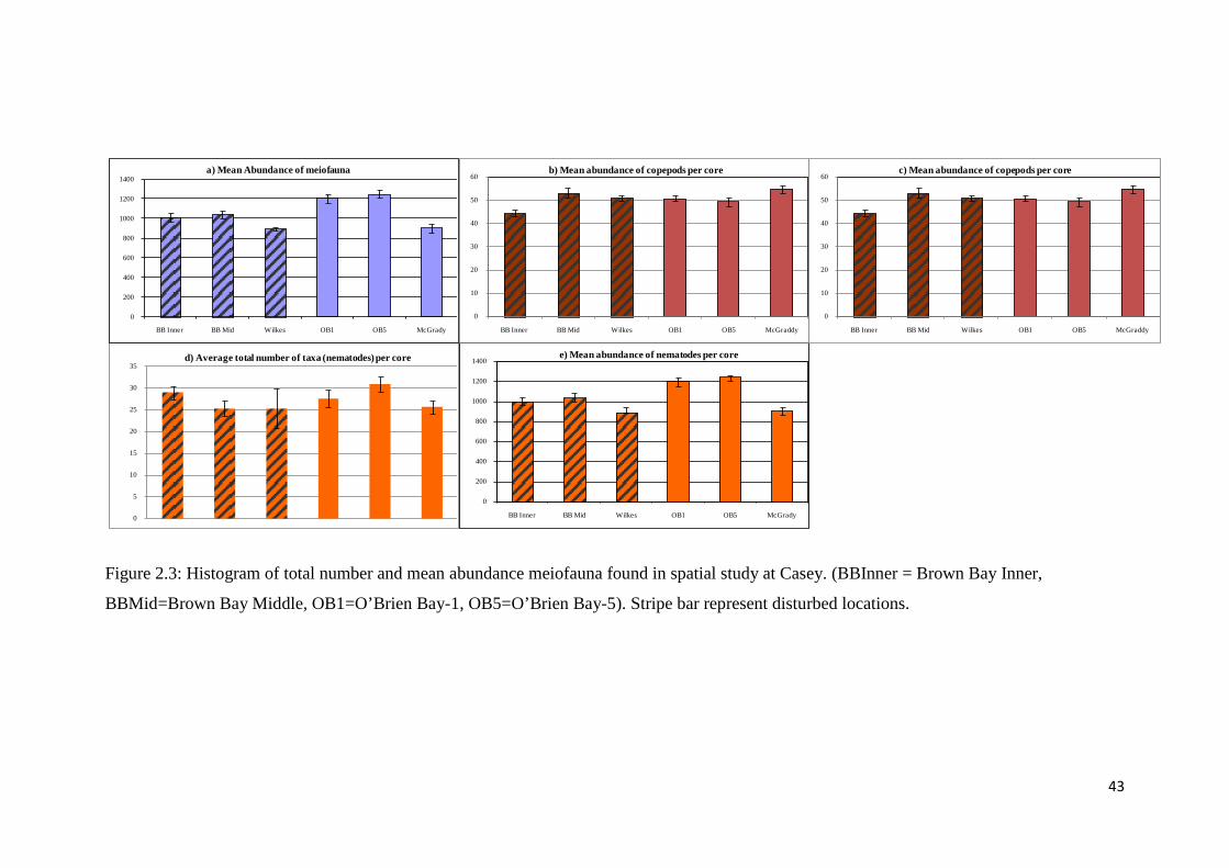
43

Figure 2.3: Histogram of total number and mean abundance meiofauna found in spatial study at Casey. (BBInner = Brown Bay Inner,

BBMid=Brown Bay Middle, OB1=O’Brien Bay-1, OB5=O’Brien Bay-5). Stripe bar represent disturbed locations.

0

200

400

600

800

1000

1200

1400

BB Inner BB Mid Wilkes OB1 OB5 McGrady

e) Mean abundance of nematodes per core

0

5

10

15

20

25

30

35d) Average total number of taxa (nematodes) per core

0

200

400

600

800

1000

1200

1400

BB Inner BB Mid Wilkes OB1 OB5 McGrady

a) Mean Abundance of meiofauna

0

10

20

30

40

50

60

BB Inner BB Mid Wilkes OB1 OB5 McGraddy

b) Mean abundance of copepods per core

0

10

20

30

40

50

60

BB Inner BB Mid Wilkes OB1 OB5 McGraddy

c) Mean abundance of copepods per core

44

2.3.2 Multivariate analysis of assemblages

Multivariate analysis of assemblage composition revealed significant differences at

several spatial scales. The nMDS ordination of all 47 samples in the spatial survey

showed distinct grouping of locations in the meiofaunal communities (Figure 2.4a).

All locations were significantly different (Table 2.1a) and in the nMDS can be seen to

form independent groups except O’Brien Bay-1 and O’Brien Bay-5, where there is

some overlap. ANOSIM results (Global R= 0.955, P< 0.01) showed the variation

within locations was less than the variation between locations (Table 2.3a and 2.4b).

Pairwise comparisons of O’Brien Bay-1 and O’Brien Bay-5 produced the smallest R

values (R=0.713), indicating that these two locations were the least different. These

two locations were separated by several kilometres and have a similar composition of

meiofaunal communities (stress value 0.17). The meiofaunal communities at O'Brien

Bay-1 and O'Brien Bay-5 showed a greater difference between sites within locations

than other locations (Table 2.3b, Figure 2.4b).

Browns Bay Inner showed no significant difference between the sites and among plots

(Figure 2.4c, Table 2.3b), however there were significant differences between sites at

Brown Bay Middle (Figure 2.4d, Table 2.3b). No other locations had significant

differences between sites with the location (Figure 2.4e-f, Table 2.3b).

45

Figure 2.4a: nMDS ordination plots based on square-root transformed meiofaunal

abundance data and Bray-Curtis similarities in Casey.

Figure 2.4b: nMDS ordination showing variability in meiofaunal community

composition between locations, sites and plots in O’Brien Bay-1 and O’Brien Bay-5.

locationsBrown Bay InnerBrown Bay MidOB1OB5wilkesMcGrady

2D Stress: 0.16

OB1 site 1 plot 1OB1 site 1 plot 2OB1 site 2 plot 1OB1 site 2 plot 2OB5 site 1 plot 1OB5 site 1 plot 2OB5 site 2 plot 1OB5 site 2 plot 2

OB1 S1P1R1

OB1 S1P1R2

OB1 S1P2R1

OB1 S1P2R2

OB1 S2P1R1

OB1 S2P1R2

OB1 S2P2R1

OB1 S2P2R2 OB5 S1P1R1

OB5 S1P1R2

OB5 S1P2R1

OB5 S1P2R2

OB5 S2P1R1

OB5 S2P1R2OB5 S2P2R1

2D Stress: 0.17

46

Figure 2.4c: nMDS ordination showing variability in meiofaunal community

composition between sites and plots in Brown Bay Inner.

Figure 2.4d: nMDS ordination showing variability in meiofaunal community

composition between sites and plots in Brown Bay Middle.

BB Inner 2BB Inner 1

Brow n Bay Inner S1P1R1








2D Stress: 0.08

BB mid 1BB mid 2

Brow n Bay Mid S1P1R2








2D Stress: 0.11

47

Table 2.3a and 2.3b: One-way ANOSIM results for compositional variation between meiofaunal communities.

Pairwise Tests (significance level used in test) R-value P-value (%) a) Location (Global R = 0.955, Significance level of sample statistic, p: 0.01%) Brown Bay Inner, Brown Bay Mid 1 0.02 Brown Bay Inner, O'Brien-1 1 0.02 Brown Bay Inner, O'Brien-5 1 0.02 Brown Bay Inner, Wilkes 0.987 0.02 Brown Bay Inner, McGrady Cove 1 0.02 Brown Bay Mid, O'Brien-1 1 0.02 Brown Bay Mid, O'Brien-5 1 0.02 Brown Bay Mid, Wilkes 0.998 0.02 Brown Bay Mid, McGrady Cove 1 0.02 Wilkes, McGrady Cove 0.991 0.02 O'Brien-1, O'Brien-5 0.713 0.02 O'Brien-1, Wilkes 0.98 0.02 O'Brien-1, McGrady Cove 1 0.02 O'Brien-5, Wilkes 0.948 0.02 O'Brien-5, McGrady Cove 1 0.02 b) Site (Global R= 0.895, significance level of sample statistic, p: 0.01%) BB Inner, Site 1 vs. Site 2 0.115 20 BB Mid 1, Site 1 vs. Site 2 0.354 2.9 Wilkes, Site 1 vs. Site 2 -0.094 65.7 O'Brien-1, Site 1 vs. Site 2 0.594 2.9 O'Brien-5, Site 1 vs. Site 2 0.611 5.7 McGrady Cove, Site 1 vs. Site 2 0.229 5.7

48

Figure 2.4e: nMDS ordination showing variability in meiofaunal community

composition between sites and plots in Wilkes.

Figure 2.4f: nMDS ordination showing variability in meiofaunal community

composition between sites and plots in McGrady Cove.

plotMcGrady 1

McGrady 2

McGrady S1P1R1

McGrady S1P1R2

McGrady S1P2R1

McGrady S1P2R2

McGrady S2P1R1

McGrady S2P1R2

McGrady S2P2R1

McGrady S2P2R2

2D Stress: 0.08

site and locationWilkes 1Wilkes 2

w ilkes S1P1R1

w ilkes S1P1R2

w ilkes S1P2R1

w ilkes S1P2R2

w ilkes S2P1R1

w ilkes S2P1R2

w ilkes S2P2R1

w ilkes S2P2R2

2D Stress: 0.06

49

2.3.3 Compositional differences between meiofaunal communities

Similarity percentage analysis (SIMPER) was used to determine the taxa contributing

to the observed differences between and within locations. The SIMPER analysis

(Table 2.4) showed that Monhystera, Daptonema and Neochromadora are among the

taxa that contributed the most to dissimilarity between locations (Figure 2.4). The

genera Monhystera and Neochromadora were found at all six study locations,

including the impacted and control locations and could be considered to be tolerant of

a range of conditions (Table 2.4). Three genera of nematodes, Sabatiera, Theristus

and Spirobolbolaimus, were considered important only in Brown Bay Inner due to

their high contribution to total abundance. In contrast, Leptolaimus, Huntemanniidae

and Cletodidae were found to be unique taxa to Wilkes. Two taxa, Promonhystera

(nematode) and Paramesochridae (harpaticoid copepod), were only found in the

disturbed locations of Brown Bay Inner, Brown Bay Middle and Wilkes. Six genera

were found only at control locations O'Brien Bay-1 and O'Brien Bay-5 and McGrady

Cove: Megadesmolaimus, Metalinhomoeus, Molgolaimus and Ancorabolidae from O'

Brien Bay; and Miraciidae and Canuellidae, harpaticoid copepods, were important

genera at McGrady Cove.

50

Table 2.4: SIMPER analysis showing family/genera ranked according to average Bray-Curtis similarity within groups. The list of genera was limited to a cumulative percentage dissimilarity of 70%. Shaded columns represent disturbed locations. Location (Ave. similarity) BB Inner (80.88) BB mid (80.61) Wilkes (74.56) O'Brien (81.44) McGrady Cove

(84.34)

Taxa Ave Contrib% Ave Contrib

% Ave Contrib% Ave Contrib

% Ave Contrib%

Monhystera 4.8 5.84 5.88 7.72 5.44 7.56 5.13 6.43 5.5 7.04 Neochromadora 3.78 4.78 4.72 6.05 4.45 6.36 2.94 3.16 4.25 5.12 Linhomoeus 3.8 4.77 2.01 2.31 Daptonema 4.05 4.73 2.1 2.06 4.95 7.01 4.53 5.61 5.54 7.17 Odonthopora 3.91 4.69 2.9 3.58 4.04 5.12 Paralinhomoes 3.19 3.81 3.5 4.51 3.78 5.45 Tisbidae 2.99 3.65 2.58 2.83 2.83 3.33 3.43 4.17 Chromadorina 2.88 3.29 3.81 4.76 2.7 3.33 2.08 2.16 3.06 3.62 Promonhystera 2.6 3.23 3.05 3.81 1.99 2.33 Chromadora 2.69 3.09 2.15 2.13 3.35 4.15 2.49 2.83 Paramesochridae 2.29 2.65 2.71 3.5 1.78 2.42 2.61 3.01 Draconema 2.33 2.65 Ascolaimus 2.37 2.64 2.35 2.61 3.25 3.89 Chromadorella 2.3 2.58 2.78 3.46 2.64 3.27 2.36 2.51 Desmodora 2.2 2.49 Wieseria 2.17 2.45 2.73 3.29 Bolbolaimus 2.22 2.33 1.97 2.28 2.64 3.06 Sabatiera 1.97 2.24 Theristus 2.13 2.21 Spirobolbolaimus 2.09 2.2 Southerneilla 2.02 2.16 2.27 2.35 Sphaerolaimus 1.94 2.09 3.16 3.87 Gammanema 2.54 3.13 2.06 2.42 Ectinosomatidae 2.34 3.03 2.47 3.55 2.21 2.65 2.57 3.29 Paracanthonchus 2.3 2.64 2.62 2.37 Paramonhystera 2.33 2.49 Canthocamptidae 1.96 2.35 1.76 2.21 Pierrickia 1.93 2.32 Ixonema 4.01 5.08 Halalaimus 3.4 4.88 2.58 3.06 4.87 6.2 Leptolaimus 3.38 4.84 Chromadorina 2.7 3.33 3.06 3.62 Dactylopusiidae 2.27 3.13 1.97 2.14 Dichromadora 2.04 2.68 2.49 2.88 Huntemanniidae 1.86 2.6 Aegisthidae 1.61 2.33 1.92 2.23 Microlaimus 2.04 2.1 2.43 2.92 Zosimidae 1.43 1.92 1.86 1.99 2.34 2.96 Chromadorita 1.69 1.84 2.66 2.54 Cletodidae 1.26 1.75 Megadesmolaimus 4.23 5.13 Metalinhomoeus 3.8 4.78 Molgolaimus 2.52 2.97 Ancorabolidae 1.78 2.09 Miraciidae 2.11 2.64 Canuellidae 2.1 2.58 Total taxa (Nematodes:Copepod)

22 (20:2)

20 (16:4)

20 (13:7)

21 (15:6)

21 (13:7)

51

Figure 2.5: Mean abundances of genera which have the highest contribution in all

locations.

0

5

10

15

20

25

30

35

40

BB Inner BB Middle Wilkes OB1 OB5 McGrady

Mea

n ab

unda

nce

Daptonema

0

5

10

15

20

25

30

35

40


Mea

n ab

unda

nce

Monhsytera

0

5

10

15

20

25

30

35

40


Mea

n ab

unda

nce

Neochromadora

52

The SIMPER analysis of the meiofaunal communities shows that the average

dissimilarity of O'Brien Bay-1 and O'Brien Bay-5 was very low (20.74%) and was

due to 43 taxa (26 genera of nematodes and 17 families of copepods) out of the 58

recorded taxa, the most dominant of which were Sphaerolaimus (3.83%), Ameiridae

(3.69%) and Rometidae (3.16%). As O'Brien Bay-1 and O'Brien Bay-5 were the most

similar locations; their distance is less than 200m., they were combined into one

group in a SIMPER analysis comparison with other locations. A total of 46 taxa (35

genera of nematodes and 11 families of copepods) contributed to the average

dissimilarity (38.76%) of the groups Brown Bay Inner and O'Brien Bay, represented

mainly by Megadesmolaimus (5.91 %), Promonhystera (3.63%), Metalinhomoeus

(3.62%) and Wieseria (3.03%). In contrast, a total of 44 taxa (31 genera of nematodes

and 13 families of copepods) contributed to the average dissimilarity (36.88 %) of the

groups Brown Bay Middle and O'Brien Bay, which were Promonhystera (4.5%),

Ixonema (4.29%), Megadesmolaimus (3.9%), Molgolaimus (3.7%) and Daptonema

(3.63%). Megadesmolaimus was more abundant in Brown Bay Inner than Brown Bay

Middle, whereas Promonhystera showed the opposite pattern.

The spatial variation of meiofaunal communities at Casey was significant at three

scales: between locations (1000’s of meters) between sites within locations (100’s

meters) and between plots within sites (10’s of meters). This study shows that the taxa

were most different at the largest scale (locations). These were supported by variance

component estimates for all scales (Table 2.5). Neochromadora, Pierrickia,

Sabatieria and Spirobolbolaimus were not significantly different at the largest scale.

Meanwhile, Daptonema, Neochromadora, Megadesmolaimus, Metalinhomoeus,

Molgolaimus, Paralinhomoes, Ancorabolidae and Canuellidae were significantly

53

different at medium scales. The taxa that were significantly different at the finest scale

were Daptonema, Ixonema, Neochromadora, Megadesmolaimus, Molgolaimus,

Monhystera, Odontophora, Paramonhsytera, Pirrickia, Theristus, Huntemanniidae,

Miraciidae and Zosimidae.

Table 2.5: Summary of significant results of ANOVA tests and post-hoc comparisons by SNK tests for taxa at different scales and estimates of variance components for three factor-nested design. Taxa Location Site Plot Variance estimates %

Location Site Plot Residual Daptonema McGrady Cove = Wilkes = OB1

= OB5 = BBInner > BBMid BBInner* BBInnerS1*

74.3 1.8 0.0 23.9 Halalaimus McGrady Cove > Wilkes > OB5

= OB1 > BBMid = BBInner NS NS

90.8 0.0 1.4 7.8 Ixonema BBMid > Wilkes = OB5

=OB1=McGrady Cove=BBInner NS BBMidS1**

BBMidS2** WilkesS1** 90.3 0.0 7.4 2.3

Leptolaimus Wilkes > BBInner > BBMid = OB5 = OB1 = McGrady Cove

NS NS 78.7 0.0 0.0 21.3

Neochromadora NS OB1* OB5*

McGrady CoveS2* 49.4 16.5 7.0 27.1

Megadesmolaimus OB1 = OB5 > BBMid = Wilkes = McGrady Cove = BBInner

OB1* OB5**

WilkesS2* 82.1 13.6 1.0 3.3

Metalinhomoeus OB1 = OB5 > Wilkes = BBMid = BBInner = McGrady Cove

OB5* Wilkes**

NS 65.9 13.9 0.0 20.2

Molgolaimus NS Wilkes* OB1S1** WilkesS2** 59.8 3.2 18.6 18.4

Monhystera BBMid >all others NS BBInnerS1* WilkesS2* 24.6 0.0 32.3 43.1

Odontophora Wilkes = BBInner > BBMid > OB1 = McGrady Cove = OB5

NS WilkesS1** WilkesS2** 55.0 0.0 24.7 20.3

Paralinhomoes BBMid > OB5 = all others BBInner* OB*

NS 68.9 12.9 0.0 18.2

Paramonhsytera BBMid > OB5 = all others NS BBMidS1* OB5S1* 65.1 0.0 22.9 11.9

Pierrickia NS BBInner* BBMidS1* 44.6 27.9 3.9 23.6 Sabatieria NS NS NS 28.2 0.0 0.0 71.8 Spirobolbolaimus NS NS BBInnerS1** 50.6 0.0 21.0 28.4 Theristus BBInner > Wilkes =all others NS BBInnerS1*

WilkesS2** 37.0 0.0 17.6 45.4 Ancorabolidae OB5 > OB1 = BBMid =

McGrady Cove > Wilkes = BBInner

BBMid* NS

71.7 4.6 0.0 23.8 Canuellidae Wilkes = McGrady Cove = OB5

= OB1 = BBMid = BBInner OB5* NS

35.5 24.7 0.0 39.9 Cletodidae Wilkes > McGrady Cove > OB5

= OB1 = BBMid = BBInner NS NS

56.7 0.0 0.0 43.3 Huntemanniidae OB5 = Wilkes = BBInner =

BBMid = McGrady Cove = OB1 NS BBInnerS1*

BBMidS2** 24.5 6.5 20.3 48.7 Miraciidae McGrady Cove = BBMid =

BBInner = Wilkes = OB5 = OB1 NS BBInnerS2**

56.7 0.0 13.2 30.1 Zosimidae McGrady Cove = OB1 > BBInner

= BBMid = OB5 = Wilkes NS OB1S2*

71.5 0.0 5.1 23.5

54

2.4 DISCUSSION

The macrobenthos and microbenthic flora have been the focus of several studies in

coastal areas at Casey Station (Stark et al., 2003b, Cunningham et al., 2003a, Stark,

2000) but the meiofauna are an important component of this benthic ecosystem about

which nothing is known. In general only limited studies have been done on the

benthic meiofauna in Antarctica e.g. (de Skowronski and Corbisier, 2002, De Mesel et

al., 2006).This study provides the first general picture of the spatial distribution and

structure of the meiofaunal communities and their variability at Casey, Antarctica.

2.4.1 General meiofaunal distribution

The results clearly demonstrate that nematodes are much more abundant by

comparison to copepod in the coastal areas at Casey. Similar results were obtained by

other studies. Whereby, meiofaunal communities are dominated by nematodes, having

at least 80% of nematode in the total abundance (Van Holsbeke, 1988, Herman and

Dahms, 1992, Fabiano and Danovaro, 1999). For example, it was reported that in

Martel Inlet, King George Island, Antarctica, at a depth of 15 m, the meiofauna taxa

was dominated by nematodes (> 60%), followed by copepods, nauplii and

polychaetes (de Skowronski and Corbisier, 2002), while in the deep waters of Halley

Bay, Weddell Sea (500-1000 m) a total of only 16 meiofauna taxa was recorded, with

nematodes comprising 90% of the total abundance (Herman and Dahms, 1992). The

average total mean density of the meiofauna at Casey (1364 individuals per 10 cm2)

55

were higher than those observed in Ross Sea, which were 1191 individuals per 10 cm2

(Fabiano and Danovaro, 1999) but lower than in Halley Bay (1677 individuals per 10

cm2), in Weddell Sea (Herman and Dahms, 1992). The differences between these

studies were mainly caused by differences in water depth where samples were taken,

since both studies (Ross Sea and Weddell Sea) were done at depth more than 500 m.

Apart of influences by water depth, equipment and collection method used may also

explain the variability in results. For example, differences in densities were visible

between organism sampled from the uppermost 3 cm of substrate using hand-corer

(Veit-Köhler et al., 2008) and sample taken at 5 cm using Van Veen grab (Kotwicki et

al., 2004) at Kongsfjorden. Although the total density showed variation, all studies

showed increases in nematode abundance was paralleled with a decrease in copepod

abundance (Kotwicki et al., 2004, Veit-Köhler et al., 2008). Table 2.6 summarise the

density of meiofauna found several locations around the world. In this current study,

the total number of meiofauna taxa recorded at Casey was 58, with 38 nematode

genera and 20 copepod families. The results contained in this study are similar to

those of Lee et al. (2001a) from the deep continental shelf of Kapp Norvegia in the

eastern Weddell Sea, where a total of 38 nematode genera were found.

56

Table 2.6: Comparison of meiofaunal communities around the world (modified from

Herman and Dahms (1992)).

Reference Area Depth range (m) Density range (N.ind cm-2)

Alongi and Pichon (1988)

Pacific- Coral Sea 298 - 1610 19-170

Bouvy and Soyer (1989)

Kerguelen Island sea-level 15,000

Bovee and Soyer (1975)

Kerguelen Island -muddy site -sand/gravel -spicule-mat

4-193 4-167 26-52

121 2,580 421

Bovee et al. (1990) Gulf of Lion 500-2,500 150-1,500 Dinet and Vivier (1977)

Atlantic - Golfe de Gascogne

2,000 2,000-3,000 4,100-4,700

539 407-500 94-305

Shirayama (1984) Western Pacific - deep-sea

2,100-8,300 37 - 1,315

Snider et al. (1984) Central North Pacific

5,800 102

Pfannkuche and Thiel (1987)

NE-Svalbard Shelf Nansen Basin

226-320 3,920

1,143- 3,439 348

Herman and Dahms (1992)

Halley Bay, Weddell Sea

340 1,960 120-3,800

Fabiano and Danovaro (1999)

Ross Sea 439-567 192-1192

Kotwicki et al.(2004)

Kongsfjorden, Svalbard

44-350 1.1-2098

Veit-Köhler et al.(2008)

Kongsfjorden, Svalbard

20 1220-1613

Present study Casey-subtidal 12-20 1195-1601

57

2.4.2 Spatial variation

Spatial variation of meiofaunal communities at Casey Station was observed between

locations (1000’s of meters) between sites within the location (100’s meters) and

between plots within site (10’s of meters). Significant differences in meiofaunal

communities were strongest found at the largest scale, between locations.

Nematodes (genus) and copepod (family) taxa appeared to be very patchy and showed

greatest significant variation at the scale of locations (large) than plots (fine).

Comparisons among locations (large scale) and plots within locations (fine scale) can

be done using lower (genus level) taxonomic resolution for nematodes and higher

(family level) taxonomic resolution for copepods. Similarly, Herman & Heip (1988)

and Warwick (1988a) found family level data of meiofauna appropriate in explaining

pollution gradients and recommended family level identification from a practical

point of view. Veiga et al. (2009) studied the meiofaunal community structure at

higher taxonomic levels and distinguished the Prestige oil spill impacted site from a

non-polluted reference site. However, Heip et al. (1988) observed significant loss of

information for nematodes only at the level of sub-orders whereas for copepods, it

occurred at family level. In a study on the macrofaunal soft sediment assemblages by

Stark et al. (2003b), significant differences were observed at all scale, and most of the

variation was associated with the largest and the smallest scale. Although, the nMDS

ordination analysis showed that there was a very distinctive pattern between control

and disturbed locations. Significant differences within location were only observed in

58

Brown Bay Middle and O’Brien Bay, while the other locations showed no

differences.

Higher abundances of meiofauna were recorded in control locations (O’Brien Bay,

except for McGrady Cove) than disturbed locations (Brown Bay and Wilkes). The

highest numbers of taxa were present at Wilkes (55 taxa) and the lowest numbers of

taxa at O’Brien Bay-1 (48 taxa). Differences in number of taxa between both

locations were mainly caused by the geographical factor, physical differences and

other anthropogenic influences since O’Brien Bay is a location furthers from human

activities sites. While, Wilkes is categorizes as disturbed location and located offshore

from a large disused tip. Impacts associated with the tip site in Brown Bay and

abandoned Wilkes dump site could increase organic input, heavy metals and

sedimentation (Stark, 2000), and these could contribute to the differences between

control and disturbed locations.

It was first proposed by Raffaelli and Mason (1981) of the use of the nematode and

copepod ratio as tool for biomonitoring. The validity of this proposal has been argued

(Coull et al., 1981) and accepted with modification by many (Moreno et al., 2008b,

Lee et al., 2001b). The ratio of nematodes to copepods of at least 4:1, which is similar

to other regions of the world, e.g. the Mediterranean (De Leonardis et al., 2008,

Moreno et al., 2008b), as well as other areas in Ross Sea, Antarctica (Fabiano and

Danovaro, 1999). However, both disturbed and controlled sites around Casey station

had higher numbers of nematodes by comparison to copepods. Hence, the usage of

the ratio solely is doubt as there are difficulties in separating the effects of pollution

59

on the ratio from the effects of other environmental variables (Lambshead, 1984) as

Stark et al (2003a), showed that the significant differences in chemical and

environmental properties between both disturbed and controlled location around

Casey station. Although numbers of nematodes were higher in all locations, the

abundance and taxa distribution were also variable between control and disturbed

locations.

There were significant differences in the meiofaunal community between locations.

Wilkes, a potentially disturbed location, was most similar to the control locations.

One possible reason for this is that the Wilkes waste dump site is much older than the

Casey site and has not been disturbed recently and does not have a melt stream

running through it. Thus, this location may have recovered from pollution impacts or

may never have been as strongly impacted as Brown Bay. Wilkes also recorded a high

percentage of copepods by comparison to other disturbed sites which was similar to

the control sites of McGrady Cove and O’Brien Bay, suggesting that the benthic

environment in Wilkes is a suitable habitat for pollutant sensitive organisms. This is

supported by the findings of Warwick, (1986) who suggested that copepods are in

generally more sensitive to the effects of pollution than nematodes. Similarly, Stark et

al., (2003b) found that the macrofaunal communities at Wilkes were similar to those

of the control sites (O’Brien Bay) in some ways but in other ways resembled an

impacted location, suggesting that perhaps it was impacted at some point in its past

since human occupation.

60

Data obtained showed that the differences between locations were greater than within

locations. However, within Brown Bay, the differences between the Inner and Middle

locations were as great as between locations separated by many kilometres (as

indicated by high R-values: R=1) even though they are only several hundred metres

apart. This is possibly due to the presence of the genus Ixonema which contributed up

to 4.0% in Brown Bay Middle but were not found in Brown Bay Inner. In addition,

the genera Gammanema and Paramonhystera were only present in Brown Bay

Middle. The position of Brown Bay Inner and Brown Bay Middle relative to the tip

site may also influence the meiofauna distribution, as Brown Bay Inner is located

nearer to the tip site (15 m) than Brown Bay Middle (300 m off shore). This finding is

in agreement with those of (Stark, 2000) who reported a variation in macrobenthos

abundance between two locations within Brown Bay, which were affected by the

pollution from the garbage tip. As for O’Brien Bay-1 and O’Brien Bay-5, both

locations showed great similarity as the R-values were only 0.713, where the

contribution of all species were about similar. In addition, both locations are located

in the same embayment which has not been influenced by any station activities.

Differences in environmental conditions due to pollution are likely to have

contributed to the differences between locations in the meiofaunal communities. For

example, the genus Sabatieria was found in Brown Bay Inner, which was known to

be contaminated from human activities. This genus is also found in areas, which has

fine sediment substrate (Vanhove et al., 1998) such as Brown Bay. Other studies have

suggested that this genus has a high tolerance to pollution or disturbance (Somerfield

et al., 1994) and survives low oxygen concentrations that are unsuitable for most other

nematodes genus. Furthermore, the genera Paramonhsytera and Theristus, which

61

were found to be tolerant to metal pollution by Gyedu-Ababio et al. (1999), were

found be important taxa in Brown Bay (Table 2.7). Gyedu-Ababio et al. (1999) also

suggest that Paramonhsytera and Theristus as a possible indicator genus of pollution.

Schratzberger et al. (2002) found that Leptolaimus was sensitive to high levels of

disturbances and Daptonema was considered as a pollutant indicator. Similar

observation on Daptonema as a non-selective feeder was also reported from Signy

Island (Vanhove et al., 1998) and Kapp Norvegia (Vanhove et al., 1999). Both genera

were recorded as important taxa in the disturbed locations at Casey.

Table 2.7: Summary of important, tolerant and indicator taxa in Casey, Antarctica.

Site Important taxa Tolerant taxa Indicator taxa O’Brien Bay (1 and 5) Megadesmolaimus,

Metalinhomoeus Molgolaimus Ancorabolidae

Monhystera Neochromadora Daptonema Chromadorina

Sensitive: Halalaimus Zosimidae

McGrady Cove Miraciidae Canuellidae

Brown Bay Inner Sabatieria Theristus Spirobolbolaimus

Pollutant: Odontophora Paralinhomoes

Brown Bay Middle Paramonhsytera Pierrickia Ixonema

Wilkes Leptolaimus Huntemanniidae Cletodidae

The genera Monhystera and Daptonema were found at all six locations. Monhystera

has a previously reported worldwide distribution, from the polar to the tropical

regions (Gerlach and Schrage, 1971, Vanhove et al., 1998, Vanhove et al., 1999,

Vanaverbeke et al., 1997, Lee et al., 2001a) and has been found abundantly in

62

organically enriched and polluted sediments (Lorenzen et al., 1987) and is known as a

colonizer genus and is considered an indicator of pollution (Veiga et al., 2009). This

characteristic explains the widespread distribution of the genus thus suggesting that

this genus is a tolerant species. Nematodes of the genus Neochromadora and

Chromadorina are also considered to be tolerant species due to their presence in all

locations. The genus Daptonema is also typically found in muddy and heavily

polluted sediments (Moreno et al., 2008a) and has been proposed to be representative

of a community that is well adapted to disturbed conditions (Brandt et al., 2007).

Finding from this study suggest that by studying meiofaunal assemblages at fine to

largest scale and identifying taxa at higher taxonomic resolution level could

distinguished the potential impacted sites around Casey region. This study also

supports the suggestion by Stark et al (2003a) that survey identification to medium

levels of resolution (family, suborder) could be done to reduce samples sorting, time

and lessen the cost. Information baseline data on opportunistic, important and

sensitive taxa could be gathered from this study for future research monitoring.

63

3.0: THE INFLUENCE OF ENVIRONMENTAL VARIABLES ON

MEIOFAUNAL COMMUNITIES AT CASEY

3.1 Introduction

The relationships between benthic macrofauna communities from polar waters and

environmental factors have been studied extensively for many years. In contrast,

studies on meiofaunal (small metazoans passing through a 500 µm mesh sieve but

retained on a sieve 32 µm) communities and the environmental factors affecting them

are still relatively poorly known, especially in Antarctica. However, the importance of

meiofauna has been emphasized in many studies (Gerlach, 1971, Alheit and Scheibel,

1982). These studies have concluded that meiofaunal communities are responsible for

stimulating microbial activity in the sediment (de Skowronski and Corbisier, 2002, De

Mesel et al., 2006, Mamilov and Dilly, 2002), they themself are food for the

macrofauna (Coull, 1990, Pihl and Rosenberg, 1984, Leduc and Probert, 2009) they

can be a potential bioindicator of environmental impacts (Moore and Bett, 1989,

Moreno et al., 2008, Sutherland et al., 2007, Kennedy and Jacoby, 1999, Gyedu-

Ababio et al., 1999, Schratzberger et al., 2001) and their production is greater than

that of macrofaunal communities.

The abundance of meiofauna is largely influenced by environmental factors such as

nutrients, salinity, sediment grain size and physical and chemical sediment

disturbances (sedimentation and pollution). These factors however, vary from large

64

scales (kilometres) to small scales (meters) (Alves et al., 2009). At larger scales (km),

the distribution of meiofauna is commonly related to abiotic gradients in sediment

composition and granulometry, salinity, temperature changes and tidal or wave

actions (Alves et al., 2009, Soetaert et al., 1995). At smaller scales (meters),

distributions are determined by the availability of food sources (Franco, 2007, de

Skowronski and Corbisier, 2002), predation (Hoste et al., 2007), reproductive

behaviour (Alves et al., 2009, Soetaert et al., 1995) and disturbance (Austen and

Widdicombe, 2006, Gallucci et al., 2008, Lee et al., 2001a) .

Although it is not yet clear which factors are most important for meiofauna

distribution in polar areas, de Skowronski & Corbisier (2002) emphasized that food

availability in the substratum and sediment grain size could be the most important

factors determining the distribution of the meiofauna in Antarctic seas. For example,

the biovolume of harpacticoid copepods was found to be related to food supply, in

terms of carbon and nitrogen availability, produced by benthic and pelagic primary

production in Potter Cove, Antarctica (Veit-Kohler, 2005). In addition, Veit-Kohler

(2005) also found that the abundance of harpacticoids had a positive relationship with

total organic matter. Effects of sediment grain size on meiofaunal distributions have

been observed in other studies (Alves et al., 2009). For example, in a study of the

intertidal sand substrata around Iceland, a positive relationship was found between

sediment properties (utilizable organic matter, fine sand fraction) and meiofaunal

abundance (Delgado et al., 2009). Although the relationship between meiofauna and

sediment grain type has been emphasized in many studies, Kotwicki et al. (2004)

observed that in the intertidal areas in Kongsfjorden, Arctic, the lack of sediment

65

stability and permanent mineral sedimentation processes also appeared to be an

influencing factor on the distribution of meiofauna.

In addition to sediment grain size and food availability, heavy metal contamination

has also been found to be a major disturbance on soft sediment assemblages in

Antarctica (Stark et al., 2003b, Cunningham et al., 2005). For example at Casey

Station, Antarctica, heavy metal and hydrocarbon contamination has been found

around two abandoned waste dumps (Stark et al., 2006, Stark, 2000, Cunningham et

al., 2003b, Stark et al., 2003b). There are significant differences here between the soft

sediment infaunal assemblages of the impacted sites and the nearby control areas

(Stark, 2000, Stark et al., 2003b). Stark et al. (2003b), demonstrated that the impacted

locations around Casey Station had lower diversity and lower species richness. They

concluded that differences in soft-sediment assemblages between control and

potentially impacted locations were closely correlated with concentrations of heavy

metals in the sediments. It has been previously shown that an increase in metal

concentration can cause a decrease in nematode diversity (Tietjen, 1980). In addition,

Somerfield et al (1994), have also shown that the nematode community structure in

the Fal Estuary, England changed consistently with increasing sediment metal

concentration, while changes in copepod abundance were more random.

To date there are limited studies examining the influence of environmental variables

on meiofaunal assemblages in Antarctica. In this Chapter, the following questions are

addressed:

66

- Are the composition, abundance and spatial variation of meiofaunal

communities at Casey related to environmental variables such as metals, grain size

and organic carbon?

3.2 Materials and Methods

Sampling design: Sediment samples were collected by divers using small core tubes

(16 mm diameter) from six locations including three control locations and three

disturbed locations, adjacent to waste disposal sites. Sampling followed a hierarchical

nested design at three spatial scales, from ~10 meters, ~100 metres to kilometres, to

determine the spatial patterns of community composition and abundance. Two

disturbed locations were situated along a gradient of pollution within Brown Bay

(Inner and Middle), the other represented by a single, potentially impacted area near

Wilkes (Figure 3.1). Within each location there were two sites (~ 100 m apart) and

within each site there were two plots (~10 m apart). Within each plot (1 m diameter),

two replicate cores were taken.

3.2.1 Location Description

Casey Station

Casey Station is situated at 66o17’ S, 110 o 32’E on Bailey Peninsula in the Windmill

Islands, Antarctica (Figure 3.1). The shallow (<50 m) benthic marine environment in

67

the near shore region at Casey is very heterogeneous (Stark, 2003). In this study, the

locations selected around Casey Station were Brown Bay (Middle and Inner), Wilkes,

O’Brien Bay (1 and 5) and McGrady Cove.

Brown Bay

Brown Bay is a small embayment at the southern end of Newcomb Bay with a

maximum depth of approximately 20 m and with rocky sides grading to a muddy

bottom (Cunningham et al., 2003b). Brown Bay is typically ice free for 1-2 months a

year, usually in January and February, and the ice does not usually break out in

winter. Brown Bay is situated adjacent to the abandoned Casey waste dump, which is

on the foreshore of the bay, at the base of Thala Valley (Stark et al., 2003c). Samples

were taken from 2 locations within Brown Bay: Brown Bay Inner was 50 m from the

waste dump directly in front of the point where summer melt water from the valley

enters the bay (Stark et al., 2006) and the water depth was 7 m. Brown Bay Middle

was 200 m from the waste dump and ranges from 12 to 15 m in depth. .

Wilkes

The first Australian station in the area, Wilkes was built in 1957 on Clark Peninsula

on the shore of Newcomb Bay but was abandoned in 1969 (Cunningham et al., 2005).

The Wilkes waste dump site is on the foreshore of a small embayment on the northern

side of Newcomb Bay. Samples were collected from approximately 100 m directly in

front of the waste dump.

68

O’Brien Bay

O’Brien is a large bay situated several kilometres south of Casey Station. This site is

clean and unlikely to have been contaminated by human activities. Therefore, the area

was selected as a reference location. The benthic habitat consists of rocky bottoms,

boulders, cobbles and gravel overlain by patches of sediment (Stark et al., 2003a).

Samples were taken in 15-20 m water depth.

McGrady Cove

McGrady Cove is a small embayment situated in the north-west corner of Newcomb

Bay. The northern shore consists of low ice cliffs (up to 5m) and the southern side of

the bay is a rocky slope. No human activities are known to have occurred in the bay

and it was intended as a reference location within Newcomb Bay. Samples were

collected on the northern side of the bay in 12 – 15 m depth.

69

Figure 3.1: Map shows the study location in Casey, Antarctica.

70

3.2.2 Heavy Metal Analysis Methods

All plastic and glassware was soaked in 10% HNO3 for 24 hours and rinsed with

Milli-Q water (resistance >18 MΩ) before use.

A partial metal extraction was used as detailed in Snape (2004) and Larner (2006).

Briefly, sediment was first sieved through a 2 mm plastic mesh and the component <

2 mm was used in extractions. Four hour extractions were conducted using 1.0 M HCl

(prepared from analytical grade HCl 32% w/w; Univar). All extractions used 1 g of

sediment to 20 ml 1 M HCl solution (1:20 w/v) and were extracted in Teflon

containers on an orbital shaker for a period of 4 h. Supernatants were immediately

filtered through 0.45 lm cellulose nitrate membranes (Sartorius) using a Millipore

filter unit into a 70 mL HDPE container and stored at 4°C until elemental analysis

using magnetic sector ICP-MS (Finnigan Element 1, Bremen, Germany, offering high

spectral resolution capability) at the Central Science Laboratory, University of

Tasmania, using a previously reported method Townsend (2000, 1999). A total of 20

elements were measured (Ag, Al, As, Ba, Bi, Ca, Cd, Co, Cr, Cs, Mn, Mo, Pb, Rb,

Sn, Sr, Th, Tl, U, Zn). Th is a rare earth element. Triplicate analysis of individual

sediment samples (range 1-14% relative standard deviation (RSD), average 5% RSD,

n=10) and analysis of certified reference materials MESS-3 and PACS-2 ensured

quality control. Detection limits (DL) were 3 σ of the blanks with As, Mo, Ni, Sb, and

Sn sometimes below DL values of 0.4, 0.03, 0.3, 0.001 and 0.01 mg kg-1 dw (dw

denotes dry weight) respectively. When measured concentrations were below DL,

values of half the DL were used in statistical analyses.

71

3.2.3 TOC – Total organic carbon analysis

Approximately 2-3 g of wet sediment, was accurately weighed, dried for 24 hours at

105 °C in a crucible and re-weighed to determine water content (WC), then placed in

a muffle furnace at 550 °C for 4 hours for organic content determination by Loss On

Ignition (LOI, Heiri et al. (2001)). Triplicate analysis of individual samples indicated

RSDs of 0.6% for WC and 2.2% for LOI (n=6).

3.2.4 Grain size

A 0.25-1 g sample of dry sediment was weighed into a clean beaker. 30 mL of 5%

Sodium Hexametaphosphate (filtered to < 0.45 micron) was added and the mixture

sonicated for 30 seconds. After a period of 24 hours, the sample was analysed using a

Malvern Mastersizer 2000 with Hydro 2000G. For this analysis, four replicates (n =

4) of grain size samples were analysed. There were 17 parameters measured. These

were TOC, 0.01 – 2µ, 2 - 7.8µ, 7.8 - 15.6µ, 15.6 – 31µ, 31 - 62.5µ, 62.5 – 125µ, 125 –

250µ, 250 – 500µ, 500 – 1000µ 1000 – 2000µ, Maximum phi, Minimum phi, Mean

um, Sorting quartile deviation, Sorting coefficient, graphic Skewness, Inclusive

graphic Skewness, Kurtosis, <2mm % and >2mm %

72


The relationship between community structure and environmental variables were

examined using the PRIMER program (Plymouth Marine Laboraties, UK) and

included use of several methods: the BEST routine, LINKTREE and RELATE. The

degree of correlation among similarity matrices was tested using RELATE analysis, a

non-parametric form of the mantel test. To estimate the threshold of environmental

variables for separation of groups of samples, linkage tree (LINKTREE) analysis, a

non-parametric modification of multivariate regression trees by De’ath (2002), was

performed using the subset of environmental variables identified by BEST analysis

(Clarke and Gorley, 2006, Clarke et al., 2008). A LINKTREE analysis was applied to

determine which abiotic variables represented the greatest differences among groups

of samples (SIMPROF test). The other statistic reported for LINKTREE analyses is

B%, which is an absolute measure of group differences from the original resemblance

matrix. When B% is large, it indicates that the split group is that percentage different

than the remainder of sites. An analysis of correlations among environmental

variables was done and where correlations were greater than 0.95, one of the variables

was removed to prevent over-parameterization.

73

3.3 Results

3.3.1 Relationships between biological and environmental parameters

Multivariate relationships between biological and environmental parameters were

examined using a variety of methods. The MDS of the meiofaunal communities

(abundances averaged over plots) can be seen in Figure 3.2. The relationship between

samples based on all environmental variables measured is shown in a PCA analysis,

which showed clear differences between locations (Figure 3.3a), but also that when all

environmental variables that were measured are considered, the resulting pattern is

very unlike the biological pattern of meiofaunal communities. Based on all measured

environmental variables, O’Brien Bay-1 was very different to all other locations.

O’Brien Bay-5 and McGrady Cove were very similar to each other as were Brown

Bay Inner, Brown Bay Middle and Wilkes. Wilkes showed the biggest difference

within locations (Figure 3.3a). An MDS of all environmental variables (based on a

Euclidean distance similarity measure) showed very similar patterns to the PCA of

environmental variables (Figure 3.3b).

Several methods were used to try to find a subset of the environmental variables that

better ‘explained” or matched the meiofaunal patterns.

74

Figure 3.2: nMDS ordinations of biota (a) meiofaunal, b) nematodes only and

copepods only.

LocationBBinnerBBmidOB1OB5WilkesMcGrady

2D Stress: 0.13


2D Stress: 0.13

a) meiofaunal

b) nematodes

c) copepods

LocationBBinnerBBmidOB1OB5W ilkesMcGrady

2D Stress: 0.16

75

Figure 3.3a: PCA ordination of all environmental variables between locations (total

variance explained by the first two principal components = 52.8 %).

Figure 3.3b: nMDS of environmental variables

-20 -15 -10 -5 0 5 10PC1

-10

-5

0

5

PC

2



2D Stress: 0.08

76

Table 3.1: Results of PCA. Eigenvectors for all variables, eigenvalues and percentage

of variation are given.

Variable PC1 PC2 Rb -0.142 0.103 Sr -0.146 -0.097 Mo -0.121 -0.137 Ag -0.089 -0.084 Cd -0.092 -0.171 Sn -0.059 -0.151 Ba -0.144 -0.056 Tl -0.079 -0.212 Pb -0.083 -0.153 Bi -0.064 0.003 Th -0.128 0.073 U -0.128 -0.133 Al -0.102 0.126 Cr -0.129 0.054 Co -0.108 0.185 Zn -0.130 -0.130 As -0.120 -0.101 TOC (LOI) -0.127 -0.154 0.01 - 2 -0.103 0.188 2 - 7.8 -0.121 0.166 7.8 - 15.6 -0.143 0.106 15.6 - 31 -0.154 -0.019 31 - 62.5 -0.136 -0.128 62.5 - 125 0.066 -0.098 125 - 250 0.156 -0.007 250 - 500 0.151 0.022 500 - 1000 0.115 0.052 1000 - 2000 0.117 -0.005 Maximum phi -0.135 0.133 Minimum phi -0.130 -0.083 Mean um 0.160 0.002 Sorting quartile deviation -0.037 0.152 Sorting coefficient 0.043 -0.145 graphic Skewness -0.129 0.055 Inclusive graphic Skewness -0.136 0.057

Kurtosis 0.067 -0.070 <2mm % -0.065 -0.024 >2mm % 0.065 0.024 Eigenvalues 36.4 12.0 %Variation 52.8 17.4

77

The relationships between biological distributions and single environmental variables

were examined by superimposing environmental variables onto the MDS of the

meiofaunal assemblages (Figure 3.4 and 3.6). Many metals were highly inter-

correlated, particularly Pb with Fe, Cu, Ni, Sb, Sn, Sr, Mn and Zn. Some of these

highly correlated metals were excluded from further analyses to prevent over

parameterization, including Cu, Fe, Cr and Sn.

There were clear relationships between many of the metals and the meiofaunal

assemblages. Some important taxa (Paralinhomoes, Halalaimus, Chromadorina )

had positive correlations with selected metals. In Brown Bay Inner, the strongest

correlation was seen between Paralinhomoes and Sn (r2 = 0.626, p = 0.097). The

Genus Halalaimus had a strong correlation with Cr at Wilkes (r2 = 0.718, p = 0.045)

and with Zn at O’Brien Bay-5 (r2 = 0.945, p < 0.001). While the genus Chromadorina

was found to have a strong correlation with Zn at Brown Bay Middle (r2 = 0.569, p =

0.141) and McGrady Cove (r2 = 0.721, p = 0.043). The Zosimidae were seen as

sensitive taxa. They were founds to have a negative correlation with Al (r2 = -0.0585,

p = 0.128), Cd (r2 = -0.730, p = 0.040) and Zn (r2 = --0.700, p = 0.053) in Brown Bay

Middle.

The potentially impacted locations, excluding Wilkes, all had higher concentrations of

heavy metals (in particular Pb, Ag, As, Cu, Fe, and Sn) than the control locations

(Figure 3.5). Wilkes had relatively high levels of Cd and Zn. The heavy metals tended

to have their greatest concentrations at locations on the top right side of the

ordination, which are represented by Brown Bay Inner, Brown Bay Middle (Figure

78

3.4) although McGrady Cove also had relatively high levels of some metals such as

Ag, U, Cd, and Zn. Vector plots of environmental variables overlaid on the MDS of

meiofaunal communities show the strong relationship between many metals and

meiofaunal communities. For example there were strong positive correlations between

the Brown Bay samples and many of the anthropogenically derived metals such as Pb,

Sn, Zn, Fe, Cu, Sn. By comparison, meiofauna from McGrady Cove showed strong

correlations with metals that most likely to have been derived from local mineralogy

such as Ba, Th, Cr, Co. (Figure 3.8a and Figure 3.8b). All sites had similar

proportions of fine sediment, < 63 µm, but Brown Bay had less fine and coarse sands

than O’Brien Bay (Figure 3.6). The average grain size was smaller at Brown Bay and

McGrady Cove, which were situated in Newcomb Bay, while the coarser and sandiest

sediments were mostly found in O’Brien Bay. Variations in grain size contributed less

to the meiofaunal distributional patterns than the heavy metals (Figure 3.7). Many

grain size classes were highly variable within locations (Figure 3.7).

79

Figure 3.4: nMDS ordinations of average value of heavy metals superimposed onto

the MDS of meiofauna assemblages.

2D Stress: 0.13Ag

As

Pb

Ba

U

2D Stress: 0.13

2D Stress: 0.132D Stress: 0.13

2D Stress: 0.13 2D Stress: 0.13

Cd

2D Stress: 0.13Sn

2D Stress: 0.13

Zn

2D Stress: 0.13

Fe2D Stress: 0.13

Cu

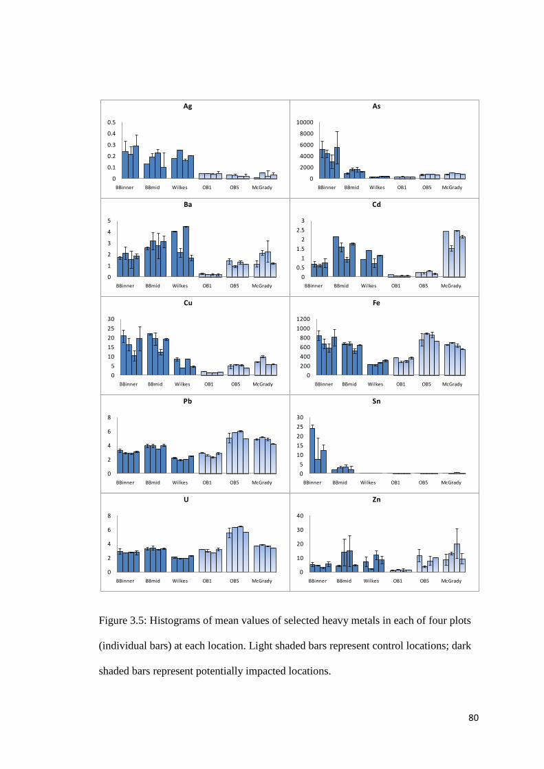
80

Figure 3.5: Histograms of mean values of selected heavy metals in each of four plots

(individual bars) at each location. Light shaded bars represent control locations; dark

shaded bars represent potentially impacted locations.

0

0.1

0.2

0.3

0.4

0.5

BBinner BBmid Wilkes OB1 OB5 McGrady

Ag

0

2000

4000

6000

8000

10000


As

0

1

2

3

4

5


Ba

0

0.5

1

1.5

2

2.5

3


Cd

0

5

10

15

20

25

30


Cu

0

200

400

600

800

1000

1200


Fe

0

2

4

6

8


U

0

2

4

6

8


Pb

0

5

10

15

20

25

30


Sn

0

10

20

30

40


Zn

81

Figure 3.6: nMDS ordinations of average value of sediment properties; grain size

(µm) and TOC (LOI) superimposed onto the nMDS of meiofauna assemblages.

2D Stress: 0.13 2D Stress: 0.13< 63 62.5- 125

125-250

500-1000 1000-2000

mean µm

250-500

TOC (LOI)




82

Figure 3.7: Histograms of mean values of sediment grain size variables in each of four

plots (individual bars) at each location. Light shaded bars represent control locations;

dark shaded bars represent potentially impacted locations.

0

5

10

15

20

25

BBInner BBMid Wilkes OB1 OB5 MG

0.01 - 2

0102030405060


2 - 7.8

0102030405060


7.8 - 15.6

0100020003000400050006000


15.6 - 31

02468

1012


62.5 - 125

0

1

2

3

4


125 - 250

0

5

10

15

20


250 - 500

0

5

10

15

20

25


500 - 1000

0

10

20

30

40

50


31 - 62.5

05

1015202530


1000 - 2000

83

Figure 3.7(cont.): Histograms of TOC and mean values of sediment grain size

variables in each of four plots (individual bars) at each location. Light shaded bars

represent control locations; dark shaded bars represent potentially impacted locations.

0

2

4

6

8


Maximum phi

0

2

4

6

8


Minimum phi

0123456


Mean υm

0

1

2

3

4

5


Sorting quartile deviation

0

1

2

3

4

5


Sorting coefficient

0

1

2

3

4

5


graphic Skewness

0

1

2

3

4


Kurtosis

0

50

100

150

200

250


<2mm %

0

1

1

2

2


>2mm %

0.0

0.2

0.4

0.6

0.8


TOC

84

Figure 3.8a: Combination of nMDS and vector shows locations were influenced by heavy metals.


1

2

3 4

5

6

7

8

9

10

11

12 13

14

15

1617

18

19

2021

22

23

24

Rb

SrMo

Ag

Cd

Sn

CsBa

Tl

Pb

Bi

Th

UAl

Ca

Cr

Mn

Co

ZnAs

2D Stress: 0.13

85

Figure 3.8b: Combination of nMDS and vector shows locations were influenced by grain size and other sediment variables.


1

2

3 4

5

6

7

8

9

10

11

12 13

14

15

1617

18

19

2021

22

23

24

TOC (LOI)

2 - 7.8

7.8 - 15.6

15.6 - 31

62.5 - 125

125 - 250

250 - 500500 - 1000

1000 - 2000Maximum phi

Minimum phi

Sorting quartile deviation

Sorting coefficient

I nclusive graphic Skewness

Kurtosis <2mm %

>2mm %

2D Stress: 0.13

86

The BEST analysis using BVSTEP (Clarke and Gorley, 2006) was used to explore

relationships between groups of environmental variables and the biotic similarity

matrix, to find a combination of variables that most closely matched the biological

patterns. BVSTEP consistently defined a group of 37 variables including minerals and

metals that contributed to combinations of variables with good correlations. The best

combination from BVSTEP was of five metals (Table 3.3). The MDS of these five

metals shows a pattern with many similarities to the biotic MDS (Figure 3.9a),

however, the locations McGrady Cove and Brown Bay Middle are overlapping. By

including three additional variables (Cd, Pb and Zn) the resulting MDS now clearly

separates McGrady Cove and Brown Bay Inner without overly affecting the

remaining pattern between locations (Figure 3.9b). The RELATE analyses (testing

matched resemblance matrices) showed that the combination of Cd, Pb and Zn in the

group of Ag, Sn, Ba, U, and As had a very similar correlation to the optimal

combination selected using BVSTEP (ρ = 0.559) (Table 3.2).

Table 3.2: BVSTEP results shows a selection of environmental variables best

explaining meiofauna community pattern.

No. Variables rho Selections

5

0.575, p < 0.001

(BVSTEP) Ag, Sn, Ba, U, and As

8

0.559, p < 0.001

(RELATE) Ag, Sn, Ba, U, As, Cd, Pb, and Zn

87

Figure 3.9: nMDS ordinations of a) biota b) selected natural minerals (Ag, Sn, Ba, U

and As) and c) anthropogenic metals (Cd and Zn).

2D Stress: 0.06

2D Stress: 0.06


2D Stress: 0.13

a) Biota

b) natural minerals

c) anthropogenic metals

88

The LINKTREE analysis was used to find the most effective way of describing the

biological-environment relationships relative to the successive use of single variables.

In the first LINKTREE analysis, the concentrations of Ag resulted in separation of

locations into two groups; however, one of the Wilkes samples was split between

groups and included with Brown Bay and McGrady Cove (Figure 3.10a). The

concentration of Ag at Wilkes, however, was much lower than at Brown Bay and

McGrady Cove, and generally the difference in Ag concentrations between the two

groups is not large. A second LINKTREE analysis excluding Ag showed that As

produced a very similar split into two groups but here the Wilkes samples now

grouped together (Figure 3.10b). The McGrady Cove (control) samples were grouped

with Brown Bay Inner, based on the concentration of U (Figure 3.10b). As this is

likely to have had little effect on the communities due to the very low concentration

and only relatively small differences between locations, a third LINKTREE analysis

was undertaken excluding Ag and U (Figure 3.10c). The results of this LINKTREE

showed that all sites were well separated into four main groups (SIMPROF test,

P < 0.01; Figure 3.10c). Here, the first split separate sites Wilkes, O’Brien-1 and

O’Brien-5 from sites McGrady Cove, Brown Bay Middle and Brown Bay Inner at

B% = 86.8, with the As concentration less than 7.32 ppm for the former site group

and greater than 8.14 ppm for the latter (Figure 3.10c, Table 3.3). The next division

separates samples from Wilkes from those in O’Brien Bay at B% = 61.4, with a

higher Cd concentration in the former sites (Figure 3.10c, Table 3.4). The control

location (McGrady Cove) was separated from Brown Bay locations at B% = 79.1,

with the former sites showing lower concentrations of Pb than the latter, but a big

difference between the two groups (Figure 3.10c, Table 3.3). The split at G,

B% = 64.2 divides Brown Bay Middle and Brown Bay Inner. Pb and Sn

89

concentrations level were higher at Brown Bay Inner and there were also some grain

size differences (Table 3.3, Figure 3.10c). The nMDS of meiofaunal assemblages was

then split based on LINKTREE analyses showing how the locations were separated

(Figure 3.11).

Figure 3.10a: LINKTREE analysis showing divisive clustering of sites from all

environmental variables based on silver (Ag).

0

20

40

60

80

100

B%

D

C

B

H

G

F

EA

BBMid 1

BBMid 4

BBMid 2BBMid 3

McGrady 1

McGrady 3McGrady 2

McGrady 4

Wilkes 1Wilkes 2Wilkes 3

Wilkes 4

OB1-1

OB1-4OB1-3OB1-2

OB5-1 OB5-3OB5-2 OB5-4

BBInner 2

BBInner 4BBInner 3

BBInner 1

Ag < 0.045 Ag > 0.051

90

Figure 3.10b: LINKTREE analysis showing divisive clustering of sites from all

environmental variables based on Arsenic (As).

U > 1.4

U < 1.22

0

20

40

60

80

100

B%

E

D

C

B

H

G

FA


Wilkes 4 OB1-1

OB1-4OB1-3OB1-2

OB5-1OB5-2

OB5-3OB5-4

BBMid 1

BBMid 4

BBMid 2BBMid 3

McGrady 1

McGrady 3McGrady 2

McGrady 4

BBInner 2

BBInner 4BBInner 3

BBInner 1

As < 7.32 As > 8.14

91

Figure 3.10c: LINKTREE analysis showing divisive clustering of sites from all

environmental variables with the exclusion of rare earth and some metals (Ag and U)

based on As.

0

20

40

60

80

100B

%


Wilkes 4OB1-1

OB1-4OB1-3OB1-2

OB5-1OB5-2

OB5-3OB5-4

BBInner 2

BBInner 4BBInner 3

BBInner 1

McGrady 1

McGrady 3McGrady 2

McGrady 4

BBMid 1

BBMid 4

BBMid 2BBMid 3

A

F

GB

E C

D

H

Pb < 2.42

Pb > 17.1

Grain size : Slightly coarser

As < 7.32 As > 8.14

92

Table 3.3: LINKTREE and SIMPROF test result.

Split Variables Location A B: As < 7.32 Wilkes, OB 1, OB 5 π = 4 P= 0.1% F: As > 8.14 McGrady Cove, BB Mid,

BB Inner R= 0.59 B% = 86.8 B C: Cd < 0.334 OB 1, OB 5 π = 5.35 TOC <3.83 P= 0.1% Mn > 8.93 R= 1.0 Zn < 12.1 B% = 61.4 Sn < 0.0249 E : Cd > 1.53 Wilkes TOC (LOI) >4.85 Mn < 7.84 Zn > 13.5 Sn > 0.144 C C: Pb < 0.576 OB 1 π = 1.13 Sn < 0.01 P= 0.1% Zn < 5.35 R= 0.81 Cd < 0.127 B% = 18.4 Cr < 1.73 Mn < 10.3 Maximum phi < 6.98 2 -7.8 < 4.02 Sorting quartile deviation < 1.04 Sorting coefficient > 0.489 7.8 - 15.6 < 6.08 Inclusive graphic Skewness < -0.306 125 - 250 > 28.9 Kurtosis > 1.08 15.6 - 31 < 9.82 250 - 500 > 10.3 TOC (LOI) < 1.78 1000 - 2000 > 0.00592 D: Pb > 0.983 OB 5 Sn > 0.0192 Zn > 11.2 Cd > 0.189 Cr > 4.07 Mn > 14.7 Maximum phi > 8.14 2 - 7.8 > 10.4 Sorting quartile deviation > 1.52 Sorting coefficient < 0.349 7.8 - 15.6 >13.5 Inclusive graphic Skewness > -0.12 125 - 250 < 16.8

93

Kurtosis < 0.893 15.6 - 31 > 15.2 250 - 500 < 7.37 TOC (LOI) > 3.08 1000 - 2000 < 0 F G McGrady Cove, π = 5.62 Pb > 17.1 Brown Bay Inner, P= 0.1% Zn > 31.2 Brown Bay Middle R= 0.66 Mn < 11.6 B% = 79.1 Sn > 1.9 62.5 - 125 > 16.1 7.8 - 15.6 < 14.7 2 - 7.8 < 9.89 [21-24] McGrady Cove 1, Pb < 2.42 McGrady Cove 2, Zn < 23.4 McGrady Cove 3, Mn > 12 McGrady Cove 4 Sn < 0.272 62.5 - 125 < 12.6 7.8 - 15.6 > 16.9 2 - 7.8 > 11.2 G [5-8] BB Middle π = 6.2 Pb < 27.5 P= 0.1% Sn < 3.64 R= 1 Mn > 10.1 B% = 64.2 As > 21.4 Cd > 0.937 Sorting coefficient > 0.481 Sorting quartile deviation < 1.06 Minimum phi > 2.18 TOC (LOI) > 7.6 Kurtosis > 1.02 H BB Inner Pb > 51.1 Sn > 7.6 Mn < 9.37 As < 19.8 Cd < 0.829 Sorting coefficient < 0.442 Sorting quartile deviation > 1.18 Minimum phi < 2.12 TOC (LOI) < 7.4 Kurtosis < 1.01

94

Figure 3.11: Splitting group of nMDS based on LINKTREE analyses.

Pb < 27.5Sn < 3.64Sorting quartile deviation < 1.06

Pb > 51.1Sn > 7.6Sorting quartile deviation > 1.18

Group G

As < 7.32 As > 8.14Location

BBinnerBBmidOB1OB5WilkesMcGrady

1

2

3 4

5

6

7

8

9

10

11

1213

14

15

1617

18

19

2021

22

23

24

2D Stress: 0.13Group A

Group B

Group C & D

Group ECd > 1.53TOC (LOI) >4.85Mn < 7.84Zn > 13.5Sn > 0.144

Cd < 0.334TOC (LOI) < 3.83Mn > 8.93Zn < 12.1Sn <0.0249

Group F

Pb > 17.1Zn > 31.2Sn > 1.962.5-125 >16.1

Pb < 2.42Zn >23.4Sn < 0.27262.5-125 <12.6

95

3.4 Discussion

The aim of this study was to assess the effects of sediment properties such as heavy

metals and grain size on the structure of the meiofaunal community assemblages at

six different locations that were categorized as either controls or anthropogenically

disturbed. By using multivariate techniques, differences in meiofaunal assemblages

between control and disturbed locations at Casey Station were found to be closely

correlated with concentrations of metals in sediments. Similar correlations between

soft-sediment assemblages and heavy metal contaminations were found in a study at

Casey Station by Stark (2003b), where the correlation between the biota matrix and a

group of five metals (Cd, Cu, Pb, Sn and Zn) was 0.65. Surprisingly, the meiofaunal

community patterns here showed little correlation with sediment grain size and TOC

content. Grain size and TOC did not seem to be a major influence on the meiofaunal

assemblages and there were no clear relationships with sediment grain size or TOC in

spite of grain size having previously been shown to be very influential on meiofaunal

community structure (Gyedu-Ababio et al., 1999, Somerfield et al., 1994, Soetaert et

al., 1995).

Sediment grain size and TOC are known to influence the concentration of metals in

sediments (Lakhan et al., 2003, Stark et al., 2003b). Although McGrady Cove was a

control location, it had similar TOC and grain size characteristics to the disturbed

locations in Newcomb Bay. In contrast, O’Brien Bay had lower TOC concentrations

and a coarser grain size. This may reflect differences in mineralogy and sedimentation

patterns between Newcomb Bay and O’Brien Bay. The disturbed locations, however,

96

were distinguished by fine sediments and high TOC and generally had much higher

concentrations of metals. For example, all sites in Brown Bay have high proportions

of very fine grain size (< 63 µm) and higher concentrations of Pb and Sn than the

controls. These grain size and TOC distributions are consistent with the observations

of Stark et al (2003b), who also noticed that locations with finer sediments tended to

have greater concentrations of TOC.

However, Wilkes (old dump site), which is one of the disturbed locations, contained a

higher proportion of coarse grain size sediment (> 500 µm) than other sites in

Newcomb Bay but still had a higher TOC concentration than O’Brien Bay, which is

similar to other disturbed locations (Figure 3.7). A positive relationship between

coarse sediment and high TOC has been associated with low abundances of

nematodes (Gyedu-Ababio et al., 1999). In the Casey area, this relationship was only

observed at Wilkes while at O’Brien Bay there was less TOC and a higher abundance

of nematodes (Figure 3.6). These results thus suggest that the meiofaunal community

at Casey Station was not heavily influenced by sediment grain size.

In contrast to grain size and TOC, metal concentrations were found to have a strong

influence on the community structure. Both anthropogenic and non-anthropogenic

metals have been found to be significantly correlated with differences in soft-

sediment assemblages (Somerfield et al., 1994). The multivariate analyses used here

showed a distinctive relationship between heavy metal concentration and meiofaunal

community structure. Ba, U, Sn, As and Ag were found in both control and disturbed

locations in this study and so can be considered to be of non-anthropogenic origin and

may have originated from erosion of soils (Dalto et al., 2006). Sn, Pb, Cu, Zn, Cd and

97

Fe are considered to be of anthropogenic origin as they were found in high

concentrations at the disturbed locations only. Fuel spills, heavy metals/metalloids

(typically Cu, Pb, Zn, Cd, Hg, As) and polychlorinated biphenyl (PCB) contamination

are derived from abandoned waste disposal sites (Tin et al., 2008). Past studies had

shown that the high concentrations of Cr, Zn, As, and Cd are clearly correlated with

low diversity of meiofauna (Schratzberger et al., 2001) and may indicate

anthropogenic impact at locations where these metals are present. These

anthropogenic heavy metal contaminations such as Sn, Cu, Pb and Fe have also been

found to have an influence on the benthic diatom community from Brown Bay

(Cunningham et al., 2003b).

In the meiofaunal community, differences have been observed between nematodes

and copepods in response to contaminant stress such as different types of heavy metal

contamination. For example, low abundances of nematodes were observed in

Portosole Harbour, Mediterranean, where concentrations of Zn, Pb, Cu, As and Cd in

the sediments were high (Moreno et al., 2009). Similarly, in this study, high

concentration of these heavy metal and low mean abundance of meiofauna were

observed at Brown Bay, Wilkes and McGrady Cove. In this current study, the genus

Halalaimus, Sabatieria and Pirrickia may be tolerant to metal pollution since these

genera were commonly found in locations with high concentration of Ag, Pb, Sn, Zn

and Cd. Somerfield et al (1994) demonstrated strong relationships between nematode

community structure and metal concentrations. Their study suggested that several

species, such as Ptycholaimellus ponticus, Sabatieria pulchra, Molgolaimus demani

and Axonolaimus paraspinosus were able to tolerate a wide range of metal

98

concentrations. It is possible that these species had developed a tolerance towards

metal pollution.

An attempt was made to identify which species were good indicators of disturbance,

either due to their sensitivity, as inferred from absence at disturbed locations, or due

to their tolerance to pollutions, as inferred from being abundant at disturbed locations.

In addition, the important taxa of disturbed and controlled locations were also

identified in Chapter 2. The species which appear to be most sensitive are:

Halalaimus (nematodes) and Zosimidae (harpacticoid copepods). They were both

found at O’Brien Bay. This finding supports the results by Essink and Romeyn (1994)

whereby Halalaimus usually inhabits less stress and stable environment. However,

this is not in agreement with Gyedu-Ababio et al. (1999), they noted that Halalaimus

has high abundant at sewage output point and location with highest metal pollution at

an estuary in South Africa. This may be due to high organic matter (high food

availability) in the seawage area. While, the taxa which were characterised as

opportunistic species in polluted locations were nematodes of the genera

Odontophora and Paralinhomoes. In a study by Moreno et al. (2008), Halalaimus,

Molgolaimus, Leptolaimus were grouped as selective deposit feeder nematodes.

Wieser (1953) has also classified these nematodes as selective deposit feeder on the

basis of buccal morphology. The genera Molgolaimus and Leptolaimus were also

found to be an important species in O’Brien Bay and Wilkes.

In a microcosm experiment by Millward et al. (2004), it was observed that different

metal treatments (Cu, Cd, Cr and Pb) did not produce any significant changes to the

99

total abundance of copepods. However, they found that in combination with diesel

treatments a significant change was elicited, which suggested that the presence of

diesel enhanced the effects of metals in sediments. They found that this effect was

most pronounced for the metals Cu and Cr. In this current study, it was observed that

the mean abundance of copepods in Brown Bay Middle and Wilkes were almost the

same as the Control locations, but in Brown Bay Inner, where higher concentration of

Cu were observed, the lowest mean abundance occurred. Brown Bay Inner is also

known to have higher hydrocarbon concentrations than Brown Bay Middle and

Wilkes (Stark et al 2005), due to its close proximity to the old waste disposal site, in

addition to the elevated heavy metal levels due to the location. The sensitivity of

copepods to copper was also seen in a field study near Chanaral beach (dumping site

of Copper mine tailing) of Northern Chile by Lee (2001b). They found that copepods

were sensitive to copper pollution and showed a high significant correlation (-0.895, P

< 0.001) between the mean number of harpacticoid copepods and labile porewater Cu

concentration.

The effects of both metal and hydrocarbon contaminations were also observed by

Cunningham et al. (2003a) on diatom communities in Brown Bay. Duquesne and

Liess (2003) found that the concentrations of Cd, Cr, Pb, Cu and Zn were found to be

significantly (p < 0.01) higher in Brown Bay than in O’Brien Bay, with Pb and Cu

concentrations about 17- and 3.5-fold higher, respectively. They also concluded that

these metals originated from the nearby tip site, which is adjacent to Brown Bay.

Likewise, Duquesne and Riddle (2002) found that the increase in metal concentrations

in the same nearshore environment was due to its position adjacent to the old waste

disposal tip site rather than to a natural background enrichment of the area.

100

It was found in this study that the Wilkes site had a different metal distribution pattern

from the other disturbed locations. At this location, the concentration of

anthropogenic metals such as Pb and Sn were low. Wilkes, however, has the highest

Cd concentrations (2.47 ppm) than other locations. This is 2.40 ppm higher than

O’Brien Bay-1, the control location. It is likely that the Wilkes site has had a different

contamination history to the other sites. The old waste tip at Wilkes contains variety

of metal objects, which includes old machinery, batteries, copper wire and tin cans.

These metal objects may have contributed to the different concentrations of Cd and

Zn at Wilkes.

McGrady Cove showed some similar meiofaunal distribution patterns to the disturbed

locations (Brown Bay) and had similar concentrations of Ag, As, Cd and many of the

rare earths. The concentration levels, were however lower than Brown Bay. But for

most metals, particularly those most likely to be of anthropogenic origin such as Pb,

Sn, Zn, Cu, and Fe, McGrady Cove showed patterns more similar to the control

location O’Brien Bay and Wilkes. Concentrations of metals at McGrady Cove may be

a combination of the local mineralogy (for rare earths) and long distance transport in

Newcomb Bay from contaminated locations such as Brown Bay (for Ag, As, Cd).

Heavy metal concentration in sediments from the different locations within the study

area mostly showed that contamination decreased with increasing distance from the

Casey tip site. Duquesne and Liess (2003), likewise found that the concentration of

Co, Cu and Pb in the water column at Casey Station were highest at the tip outlet and

decreased as the distance from the tip increased.

101

Arsenic (As) was also found to be strongly influential on meiofaunal community

patterns at Casey. This metal was found at higher concentrations in McGrady Cove

(26.00 ppm), Brown Bay Inner (16.21 ppm) and Brown Bay Middle (23.43 ppm).

Lower values were found in Wilkes (2.00 ppm), O’Brien Bay-1 (2.00 ppm) and

O’Brien Bay-5 (2.00 ppm). The presence of As may be have been contributed by

nearby relict penguin colonies as As has been found to be enriched in sediments

effected by penguin droppings by about two times above background levels (Yin et al.

(2006). This relationship between As and proximity to relict penguin colonies

however was not tested in this study. The source of As in the sediments in the

current absence of penguins may be attributed to the weathering and erosion of the

relict colonies, atmospheric deposition of dust and sediment from the colonies or

anthropogenic contribution from nearby sources (Yin et al., 2006).

Although the metal contaminants are present in the marine environment at Casey

Station , they are very low by comparison to Australian Environmental Standards

(Table 3.5). However, to date there are no guidelines for Antarctica soil and coastal

ecosytems.

102

Table 3.4: Comparison of selected metal/metalloid levels found in this study and

Australian Environmental Standard (Source: National Environment Protection

(Assessment of Site Contamination 1999))

Metals/Metalloids Antarctic sediments (this study). Min and max value (in ppm)

Australian Health Investigation Levels (Soil) mg/kg- Standard residential

Arsenic 2.00-45.65 100 Cadmium 0.05-2.58 20 Chromium 0.80-31.16 100 Copper 0.87-50.80 1000 Lead 0.10-0.60 300 Manganese 5.38-17.31 1500 Nickel 0.63-1979 600 Silver 0.01-0.31 No information Thallium 0.15 No information Tin 0.38-113.08 No information Zinc 3.37-53.56 7000

Metals originating from soil erosion have apparently little effect on meiofauna,

whereas some metals originating from human activities have a negative correlation

towards meiofauna total density (Dalto et al., 2006). These heavy metals have

affected the mean abundance of meiofaunal taxa, with lower numbers being were

recorded at all disturbed locations. From the results obtained here, it is clear that the

lower meiofaunal abundance and/or change in genus composition are linked to the

concentration and type of heavy metal pollutants in the sediment. It is however

unknown which heavy-metal actually has the greatest influence on the meiofauna

community in Casey since most heavy metals were present at all locations.

Mahmoudi et al. (2007) demonstrated in a microcosm experiment that contamination

with a combination of lead-zinc produced a more diverse nematode communities than

those treated by only lead or zinc. This pattern was also observed by Gyedu-Ababio

and Baird (2006), where sediment treated with Cu, Fe, Pd, Zn produced a higher total

103

meiofauna density than those treated with Pb and Zn separately, suggesting that the

synergistic effects of the metals may be more influential on the meiofauna

communities. Furthermore, Fichet et al. (1999) showed that heavy metal uptake by

nematodes and copepods were similar for Cu and Zn, while Cd and Pb were

significantly higher in nematodes than copepods.

It is known that several characteristic of meiofauna cause them to respond rapidly to

changes in the environment. Previous studies have shown that there is a close

relationship between meiofauna and the sediment matrix, thus changes in interstitial

chemistry will rapidly lead to alterations in meiofaunal abundance and diversity. This

response is particularly rapid in benthic ecosystems with sediments with finer grains

sizes. It has been well established that heavy metals are mostly associated with the

finer grain size fractions and in this study also it was observed that disturbed locations

had finer sediments and higher metal concentrations, while the locations with coarser

grain sizes had lower metal concentrations. This study only measured metal

concentrations in sediments but hydrocarbon contamination is also known to occur in

marine sediments around Casey Station (Deprez et al., 1999, Stark et al., 2005).

Studies at Casey station (Stark et al., 2003c, Cunningham et al., 2003b) have shown

significant differences in soft sediment assemblages between locations adjacent to an

abundant waste dump contaminated by heavy metals and hydrocarbons (Brown Bay)

and control locations. Therefore, hydrocarbon contamination is undoubtedly also

contributing to patterns of meiofaunal composition as metals and hydrocarbons are

frequent co-contaminants in sediments.

104

Further comparison between findings from this study and other studies are hampered

by lack published information on the relationship of meiofauna and metal

contaminations in the field. The majority of studies with meiofauna and metals have

been conducted in microcosm experiments (Mahmoudi et al., 2007, Ellis et al., 2001,

Austen and McEvoy, 1997, Millward and Grant, 2000, Millward et al., 2001, Fichet et

al., 1999, Lee et al., 2001b, Ser, 1991, Beyrem et al., 2007, Austen et al., 1994). These

laboratory experiments have tended to show that changes in meiofaunal diversity

occurs in relation to the response to specific metal contamination. In this field study,

such a conclusion could not be made since the effects are combination of various

heavy metals and possibly other unmeasured contaminants such as hydrocarbons. In

conclusion, this study has demonstrated that the composition of meiofaunal

communities near Casey Station is more highly correlated with heavy metals than to

grain size. A suite of metals consisting of Ag, Sn, Ba, U, As, Cd, Pb, and Zn were

identified as the dominating influence on the meiofaunal communities. This finding

supports the suggestion that changes in meiofaunal communities could be use a

biomonitors of heavy metals in subtidal ecosystem. A further investigation, is

however, needed in order to determine which heavy metals and at what concentration

they could affect Antarctic meiofaunal communities.

105

4.0 THE EFFECTS OF HYDROCARBONS ON MEIOFAUNAL

COMMUNITIES

4.1 Introduction

Marine benthic ecosystems are not only subjected to pollution in areas which are

highly developed, but pollution is also becoming a threat to the most clean and

pristine continent, Antarctica. A small pollution event in Antarctica can have greater

significance than occurrences of similar magnitude elsewhere in the world (Clarke

and Harris, 2003). The principal forms of human activity in Antarctica are limited to

scientific research, fishing, and tourism. The increase in human activities in certain

areas of the continent has raised concern about the pollution status and impact to

coastal ice-free rocky areas of these activities. Threats from tourism and scientific

research are currently small (Clarke and Harris, 2003), and the issue that is of most

concern to the benthic communities of Antarctica is the effects of pollution such as

heavy metals and hydrocarbons.

4.1.1 Sources and threats of hydrocarbon pollution on benthic ecosystems

Hydrocarbon pollution originates from a variety of different pathways such as

shipping and local inputs from research stations (Cripps and Priddle, 1991). There

have been a series of oil spills in Antarctica from shipping activities. The biggest oil

106

spill in Antarctica was in 1989 when an Argentine resupply vessel, Bahia Paraiso,

with tourists onboard, ran aground in the Bismarck Strait two miles from a scientific

research station operated by the United States, near the tip of the Antarctic Peninsula,

spilling about 600,000 liters of fuel. In 2001 a Chilean ship, the Patriarche,

contracted by Ecuador to resupply its Antarctic area station ran aground and spilled

petrol off the north-west Antarctic coast. The most recent spill was from the MS

Explorer, an adventure travel ship which sank in Antarctic waters after hitting an

iceberg on November 2007 carrying about 50,000 gallons of diesel, 6,300 gallons of

lubricant and 260 gallons of gasoline onboard the vessel. There is also a risk of

hydrocarbon spills from station fuel storage and resupply operations although is not

considered high. However, in 1990, a spill of 91000 L of special Antarctic blend

(SAB) diesel fuel occurred from a fuel storage facility at Casey Station (Deprez et al.,

1999).

Petroleum hydrocarbons from oil spills and other sources are a potential threat to the

coastal environment. Numerous affects to benthic marine life and the environment can

be caused by hydrocarbon pollution, for example, smothering of intertidal and benthic

organisms, changes in water temperature, toxicity of different compounds and

additives in hydrocarbons, reduced access to food and elevated nutrient

concentrations can all modify ecosystems.

To date numerous studies have been conducted to determine the affects of

hydrocarbon pollution on benthic ecosystems (Voudrias and Smith, 1986, Cripps and

Priddle, 1991, Danovaro et al., 1995, Stark et al., 2003b). Past research has shown that

107

several areas of the coastal environment around Casey Station have been

contaminated with heavy metals and petroleum hydrocarbons (Cunningham et al.,

2003). A study by Stark et al. (2003) found that the Casey research station has caused

impacts that are detectable in the adjacent marine environment. Pollution sources at

Casey Station include the old waste disposal site, the current sewage outfall and fuel

spills.

4.1.2 Responses of the benthic community to hydrocarbon pollution

The level of impacts of oil on benthic organisms depends on the concentration of oil,

oil type, and the sensitivity of the organisms concerned (Ingole et al., 2006). For

example it has been found that, Total Petroleum Hydrocarbon (TPH) has a negative

correlation with meiofauna and microfauna abundance but a positive correlation with

microbial abundance (Ingole et al., 2006). For example, in a mesocosm experiment

conducted by Beyrem et al (2009), sediment treated with mineral oil (Mobil 20 W-50)

and synthetic lubricant ( Mobil 0 W-40) showed a significant decrease in total

nematode abundance (I), species richness (d) and number of species (S) after five

days exposure. The effects of hydrocarbon pollution have been found to be more

serious for faunal living on the surface of sediment than for those burrowing into the

sediments (Cabioch, 1980). It has also been found that sites which have been

previously affected by fuel or diesel spill have a low number of copepods and a higher

density of nematodes. (Veiga et al, (2009).

108

4.1.2 Meiofauna as an indicator of pollution

Marine benthic fauna and flora have been used as indicators of stress and pollution

due to their sensitivity, especially the benthic invertebrates (Calabretta and Oviatt,

2008). They are good indicators of organic pollution due to their constant presence,

life cycle, and inactive habit. One of the main components of benthic communities

that have been widely used as an indicator is the meiofauna (Kennedy and Jacoby,

1999, Schratzberger et al., 2001, Raghukumar et al., 2001, Beier and Traunspurger,

2001). Meiofauna are an essential component of marine benthic sediment

communities, providing ecosystem services such as sediment bioturbation and

recycling of organic matter (Higgins and Thiel, 1988). Meiofauna have also been

shown to be good indicators of environmental pollution (Moreno et al., 2008). These

small and abundant organisms are bound to the sediment throughout their life history

and are often sensitive to environmental changes. Other studies have demonstrated

that the abundance and diversity of the meiofauna communities are correlated with

sediment particle size (Veit-Köhler et al., 2008, Vanhove et al., 2004), food

availability (Armenteros et al., 2006) and other environmental parameters (Doulgeraki

et al., 2006, Vanhove et al., 1995). The tolerance and occurrence of meiofauna in

polluted areas are genera specific but some genera can be classified as indicators. The

response of meiofauna is also dependant on the level of contamination (Hedfi et al.,

2007). Research has indicated that copepods show more sensitivity towards pollution

than nematodes in the meiofaunal community (Moore and Bett, 1989, Warwick, 1986,

Sutherland et al., 2007, Lee et al., 2001, Shiells and Anderson, 1985).

109

Methods using meiofauna to assess the impacts of anthropogenic stressors are not as

well developed relative to methods using macrofauna; currently available meiofauna

based methods are only applicable in sandy beach habitats experiencing organic

enrichment (Coull and Chandler, 1992). Parker (1975) and Raffaelli and Mason

(1981) have proposed using the ratio of nematodes to copepods (N/C ratio) as a

monitor of pollution or sediment changes that eliminates the need for detailed, time

consuming species identification. While, this idea is very attractive it has generated

considerable controversy (Warwick, 1981, Lambshead, 1984, Raffaelli and Mason,

1981, Platt et al., 1984, Coull et al., 1981) and it has not been proven to be an accurate

predictor of environmental change. While, the technique is simple because no

taxonomic experts need be sought, further research is needed to determine the

universality of the N/C ratio as a measure of environmental perturbation. Because of

rather difficult taxonomy of meiofauna; many perturbation studies prefer not to

include them.

To investigate the effects of hydrocarbons on Antarctic meiofaunal communities a

manipulative field experiment was undertaken in which four different types of

hydrocarbons (three synthetic lubricant oils and diesel fuel treatments) were added to

marine sediments. These were deployed in a shallow marine bay and sampled at

intervals to determine the effects of hydrocarbons and the response of meiofaunal

communities over time.

110

The aims of the experiment were:

To examine the effects of four different types of hydrocarbon treatments

(Clean lubricant oil, Used lubricant oil, Biodegradable lubricant oil and

Special Antarctic Blend Diesel fuel) on sediment meiofaunal communities.

o To investigate the distribution and diversity of meiofaunal

communities in each treatment and at each time.

o Determine which types of lubricants will most affect the

meiofaunal communities

o Examine how meiofaunal communities change through time

111

4.2 METHODS

In this study, the environmental variables data; Total Petroleum Hydrocarbon (TPH),

grain size and heavy metals data were provided by Human Impact Group, Australian

Antarctic Division (AAD) from their SRE4 monitoring project in Casey Antarctica.

4.2.1 Experimental Procedures

Field methods

An experiment was setup in which four different hydrocarbons (SAB diesel fuel, and

Clean, Used and Biodegradable lubricant oils) were added to defaunated marine

sediments and deployed in trays in a sheltered area in O’Brien Bay (Figure 4.1). The

communities colonizing the sediments were monitored for up to five years. Clean

sediments were collected from a reference location (O’Brien Bay) and treated with

one of four different types of hydrocarbons: a) Biodegradable synthetic lubrication oil

(TITAN GTI 1 (0W/20); Fuchs/rapeseed oil), b) Used synthetic lubrication oil (SAE

0W/40; Mobil) – used in CATERPILLAR machine for 150 engine hours, c) Clean

(unused) synthetic lubrication oil (SAE 0W/40; Mobil) and d) Special Antarctic Blend

(SAB) light diesel fuel. The Mobil SAE0W/40 oil is widely used at Casey and other

Australian Stations in power generators and other plant and machinery and the

Biodegradable oil is being considered as a possible alternative. In the past used oil

was dumped onto the old waste disposal site and is occasionally spilled. SAB diesel is

the main fuel used on Antarctic stations to run most plant and machinery and is stored

112

in large above ground fuel tanks and drums. The site, set-up and sampling of this field

experiment have been described in detail previously (Thompson et al., 2006, Powell

et al., 2005b).

The experiment was set up at O’Brien Bay with a layout (28 m x 18 m) divided into

24 blocks (3 m x 3 m) that were 2 m apart. Uncontaminated sediment was collected

from a different locality to the deployment site in O’Brien Bay. Sediment was sieved

through a 500 μm mesh using clean sea water (Thompson et al., 2007). Sediment was

collected by divers then transported back to the laboratory for spiking procedure

before deployed to the experimental site. Plastic trays made of a 1cm2 mesh (tray

dimensions 34 cm×23 cm×12 cm) were lined with a 300 μm mesh, and filled with

sediment treated with lubricants or diesel. They were deployed carefully to the seabed

level at depth of 15 to 18.5m. Trays were positioned on the sediment surface and

were in full contact with the sediment on the tray base. The sediment depth in each

tray was initially 10 – 11 cm, but after time there was some settling of sediments and

total depth of sediment decreased to approximately 8 cm. Five trays were located

within each block (i.e. one of each treatment and a control) and trays from four

replicate blocks were retrieved at each sampling time. The sediments were sampled

for meiofauna at 56 (T2), 102 (T4) and 260 (T5) weeks after deployment. Samples

were taken with a small corer (a 60 ml syringe with the end cut off, surface area =

5.599 cm2) by divers, with two replicate cores per tray. Cores were emptied into 70 ml

jars and preserved in 10% formalin.

113

Figure 4.1: Map shows the location of experimental site (O’ Brien Bay) in Antarctica.

114

4.2.2 Meiofauna preparation and identification

The preserved sediment was initially sieved through a 500 μm sieve to remove the

coarser sediment fraction. Samples were rinsed thoroughly with tap water to prevent

flocculation of Ludox, over a sieve of 32 µm. The sample was transferred from the

sieve to a large centrifuge tube. Ludox solution (60% Ludox and 40% water; density

= 1.18) was added to tube until the level of mixture was balanced for centrifuging.

Then the sample was centrifuged at 2800 rpm for 10 min. The supernatant was

decanted and collected and the remaining sediment pellet was resuspended. This

process was repeated three times.

All supernatants were filtered through a 100 µm sieve, followed by a 32 µm sieve.

The supernatant was finally rinsed over a 32 µm sieve with tap water for some time

because Ludox and formalin will react and form a white gel that is difficult to wash

out. After the extraction, 4% formaldehyde was added again to the treated sample.

The organisms retained by the 32 µm sieve were fixed in 4% formaldehyde. The

counting process was facilitated by staining of the entire sample with 1% of Rose

Bengal.

All animals retained on a 32 µm sieve were counted and sorted into major taxa. The

major taxa (Nematoda and Copepoda) were counted using a dissecting microscope at

25x magnification (ZEISS Stemi 2000; Zeiss Inc., Germany). Per sample, 200

nematodes (or all nematodes when density less than 200 individuals.) were picked out

115

at random and mounted on slides in glycerine after a slow evaporation procedure

(modified after Riemann, 1988) for identification to genus level mainly using Platt

and Warwick (1983, 1988) and NeMys online identification (Deprez et al., 2005). All

copepods were picked out and mounted on slides in glycerine without evaporation for

identification to family level using THAO: Taxonomische Harpacticoida Archiv

Oldenburg (2005), Huys et al. (1996) and Bodin (1997). The identification of

nematodes and copepods were done using 1000 times magnification.

4.2.3 Total Petroleum Hydrocarbon Analysis

A homogenized sub sample of approximately 5 g of sediment from the top 1 cm slice

from each core was extracted overnight with 10 ml of deionized water, 9 ml of

dichloromethane and 1 ml of dichloromethane containing as internal standards (IS) 1

mg l-1 of cyclooctane, 1 mg l-1 of bromoeicosane, 0.25 mg l-1 of 1,4-dichlorobenzene,

0.25 mg l-1 of deuterated tetracosane and 0.1mg l-1 p-terphenyl. The samples were

centrifuged for 10 mins at 3,000 rpm at 10˚C and the supernatant removed to a clean

vial. The supernatants were analyzed for total petroleum hydrocarbons (TPH) by gas

chromatography-flame-ionization detector (GC-FID) on a Varian CP3800 (Varian)

with a BP-1 (SGE) column (25 m; i. d. 0.22 mm; 0.25 μm film) and a Varian 8400

autosampler controlled with Star Chromatography Workstation. One microliter of

extract was injected (1:20 split using a 1079 PTV injector) at 1.3 ml min-1. The

detector flow rates were 29 ml min-1 for nitrogen, 30 ml min-1 for hydrogen and 300

ml min-1 for air. The oven temperature was initially 40˚C held for 3 mins, then

increased at a rate of 18˚C min-1 to 330˚C and held for a total run-time of 23 mins.

116

The TPH concentrations were determined using calibration curves based on standards

prepared with each of the oils at concentrations of approximately 8000, 5000, 2500,

1000, 500, 200, 100, 50 and 0 mg kg-1. Using the IS response relative to the total

detector response to all hydrocarbons, the TPH: IS ratio could be measured. This ratio

was also calculated for the samples and used to determine the TPH values.


Univariate analysis

A two factor experimental design was used to analyse abundance data (by ANOVA)

and community data (by PERMANOVA), with Time (3 times) and Treatment (5

treatments) as orthogonal factors. Cochran’s test was used to test for homogeneity of

variances in ANOVAs. If variances were heterogeneous, data were transformed

(Snedecor and Cochran, 1980, Underwood, 1981). Where significant heterogeneity of

variances could not be removed by transformation, a lower significance level of P =

0.01 was used. When a significant effects were encountered, post-hoc multiple

comparisons among means using the Student–Newman–Keuls (SNK) test (at a=0.05)

were carried out.

Multivariate analysis

Multivariate analyses of community composition were undertaken using non-metric

multi dimensional scaling (nMDS), Analysis of Similarities (ANOSIM) and similarity

percentages (SIMPER) procedures using the PRIMER v6.0 statistical software

117

package (Clarke and Gorley, 2006) and PRIMER + PERMANOVA (Anderson et al.,

2007). Stress values in nMDS provide a measure of goodness of fit for the ordination

with values ranging from 0 to1 (Clarke, 1993). Values close to 0 indicate a good fit

whereas a stress value greater than 0.3 is no better than arbitrary (Clarke, 1993). The

Bray-Curtis distance measure was used to determine similarities between samples,

after square-root transformation of abundance data.

PERMANOVA and one-way ANOSIM was performed to determine whether there

were significant differences among groups and to compare the similarities in the

composition of meiofaunal communities from six locations. Pairwise R-values give an

absolute measure of how separate groups are on a scale of 0 (indistinguishable) to 1

(all similarities within groups are less than any similarity between groups).

SIMPER analyses were used to determine which taxa were responsible for

compositional differences observed between meiofaunal communities. Clarke and

Warwick (1994) stated that as a guideline, species which have a SIMPER ratio greater

than 1.3 are likely to be useful for discriminating between groups.

Data transformation was applied in analyses to validate statistical assumption for

parametric techniques and to weight the contributions of common and rare taxa in the

multivariate representations (Clarke and Warwick, 2001). The transformations play an

important role to balance between contributions from common and rarer family/genus

in the measure of similarity of two samples (Clarke and Warwick, 2001). The square-

root transformation has a similar effect in reducing the weighting of abundant

118

family/genera but has the advantage that, when similarity is assessed by the Bray-

Curtis measure, the similarity coefficient is invariant to a scale change (Field et al.,

1982). A square-root transform was applied to the community composition and

nematode abundance data as this study not have high abundances of a single species

(rarely had abundances over 30 of any taxa). The log transformation has the powerful

effect of ‘scaling down’ very abundant family/genus and thus increasing equitability

of the datasetLog transformation was applied copepod abundance data because to

down weight contributions from both common and rare taxa.

4.3 RESULTS

4.3.1 Lubricant contamination

The Total Petroleum Hydrocarbon (TPH) concentrations (mg/kg) in the top 1 cm of

sediments contaminated with Clean, Used, Biodegradable, and SAB diesel decreased

from 0 weeks to 260 weeks (Figure 4.2a). In the Control, TPH increased after the

experiment started and decreased after 56 weeks and again increased slightly after 104

weeks (Figure 4.2a and 4.2b). The maximum TPH concentrations in Control

sediments after deployment were less than 73 mg/kg. In this study, the highest TPH

recorded in T2 for all four hydrocarbon treatments was in Biodegradable (5166

mg/kg) while the lowest was found in SAB diesel (1046 mg/kg). After 260 weeks, the

TPH concentrations in all treatment were still high compared to the Control. The

highest TPH concentration after 260 weeks was in Used lubricant treatment which the

value of 1046 mg/kg.

119

Figure 4.2a: Total petroleum hydrocarbon (mg/kg) concentrations in the top 1cm of sediments treatment; Control, Biodegradable, Clean,

Used and SAB diesel at 0, 5, 56, 65, 106 and 260 weeks. (Source: Human Impact Program, Australian Antarctic Division 2009)

0

2000

4000

6000

8000

10000

12000

T0 T1 T2 T3 T4 T5 T0 T1 T2 T3 T4 T5 T0 T1 T2 T3 T4 T5 T0 T1 T2 T3 T4 T5 T0 T1 T2 T3 T4 T5

Control SAB Biodegradable Clean Lubricant Used lubricant

Mean TPH (mg/kg dry)

120

Figure 4.2b: Total petroleum hydrocarbon (mg/kg) concentrations in the top 1cm of sediments treatment; Control, Biodegradable, Clean,

Used and SAB diesel in this study at 56, 106 and 260 weeks.

0

1000

2000

3000

4000

5000

6000

Control SAB Biodegradable Clean Lubricant Used Lubricant

Mean TPH mg/kg dry

T2

T4

T5

121

4.3.2 Composition of the meiofaunal

A total of 10,633 individuals from 65 higher meiofauna taxa comprised of 40 genera of

nematodes and 25 families of harpacticoid copepods were identified in 120 samples from

five treatments (Control, Clean lubricant oil, Used lubricant oil, Biodegradable lubricant

oil and SAB diesel) over 260 weeks experiment time (T2, T4 and T5). These

hydrocarbon treatments had a strong impact on meiofaunal community, affecting both

nematodes and copepods composition (Table 4.1). The highest abundances were recorded

in the Control treatment (average density ranges from 3811 to 8209 ind. 10 cm-2). Lowest

value were observed in the SAB (2251 to 4453 ind. 10 cm-2).

There was significantly difference between time and treatments in Shannon–Wiener

diversity (H’) (ANOVA, P < 0.01), species richness (Margalef’s d) (ANOVA, P < 0.01)

and evenness (Pielou’s J’) (ANOVA, P < 0.01). All indexes were lower in T2 in most

treatments and they gradually increase as duration increases (Figure 4.3).

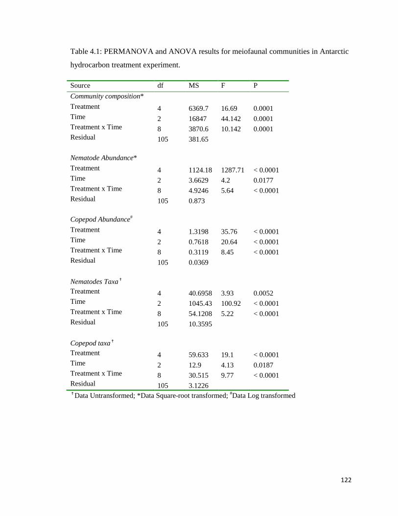
122

Table 4.1: PERMANOVA and ANOVA results for meiofaunal communities in Antarctic

hydrocarbon treatment experiment.

Source df MS F P Community composition* Treatment 4 6369.7 16.69 0.0001 Time 2 16847 44.142 0.0001 Treatment x Time 8 3870.6 10.142 0.0001 Residual 105 381.65 Nematode Abundance* Treatment 4 1124.18 1287.71 < 0.0001 Time 2 3.6629 4.2 0.0177 Treatment x Time 8 4.9246 5.64 < 0.0001 Residual 105 0.873 Copepod Abundance# Treatment 4 1.3198 35.76 < 0.0001 Time 2 0.7618 20.64 < 0.0001 Treatment x Time 8 0.3119 8.45 < 0.0001 Residual 105 0.0369 Nematodes Taxa Treatment 4 40.6958 3.93 0.0052 Time 2 1045.43 100.92 < 0.0001 Treatment x Time 8 54.1208 5.22 < 0.0001 Residual 105 10.3595 Copepod taxa Treatment 4 59.633 19.1 < 0.0001 Time 2 12.9 4.13 0.0187 Treatment x Time 8 30.515 9.77 < 0.0001 Residual 105 3.1226 Data Untransformed; *Data Square-root transformed; #Data Log transformed

123

Figure 4.3: Mean abundances (+SE) Shannon–Wiener diversity (H’ log e), species

richness (Margalef’s d) and evenness (Pielou’s J’).

0123456789

10

Control Clean Used BioD SAB

Margalef's Richness, d

T2

T4

T5

00.10.20.30.40.50.60.70.80.9

1


Pielou's Evenness, J'

T2

T4

T5

0.0

0.5

1.0

1.5

2.0

2.5

3.0

3.5

4.0


Shannon-Wiener's Diversity, H'(loge)

T2

T4

T5

124

There was a significant effect of hydrocarbon treatments on meiofaunal mean abundance,

largely due to nematodes, which comprised the bulk of the community. The highest mean

abundance of meiofauna was in Control and Biodegradable treatments, while SAB

treatments showed lowest mean abundance (Figure 4.4a). A comparison of time exposure

among treatments showed that the mean abundance of meiofauna in each treatment

changed very little over time, and was significantly greater in the Control and

Biodegradable treatments, which were not significantly different (Figure 4.4b). Mean

abundances were significantly lower in clean, used and SAB treatments at all times

(Figure 4.4b). A clear trend was observed in SAB Lubricant from T2 to T5, with a small

but significant decline in mean total abundance of meiofauna, which was largely due to a

decline in nematode abundance (Figure 4.3d). The ANOVA results indicate no

significant difference in Control and Biodegradable in the mean abundance of nematodes

(Table 4.2). Nematode diversity (no. of genera) increased from T2 to T5 in all treatments

(Figure 4.4b) (ANOVA, P < 0.001; Table 4.1 and 4.2). An increase in the number of

genera of 25% to 50% was seen in treatments over time (Figure 4.4b).

Copepods showed a very different response to hydrocarbon treatments than the

nematodes. Diversity and abundance were greater in the Control than the other treatments

at T2 and T5, but with a very different pattern at T4, with greatest diversity and

abundance in the Used treatment (Figure 4.4d, Table 4.2). The mean abundance of

copepods was highest at T4 in all the hydrocarbon treatments, when there was a

significant increase, followed by a decrease to T5 (Figure 4.4e). This pattern was not

observed in the control.

125

Figure 4.4a: Mean abundance meiofaunal and numbers of taxa found in hydrocarbon treatment experiment in Casey.

0

200

400

600

800

1000

1200

1400

Control Clean Used Biodegradable SAB

a) Mean abundance of meiofauna per core

T2

T4

T5

0

5

10

15

20

25


d) Average total number of taxa (copepods) per core

T2

T4

T5

0

5

10

15

20

25

30

35

40


b) Average total number of taxa (nematodes) per core

T2

T4

T5

0

200

400

600

800

1000

1200


c) Mean abundance of nematodes per core

T2

T4

T5

05

1015202530354045


e) Mean abundance of copepods per core

T2

T4

T5

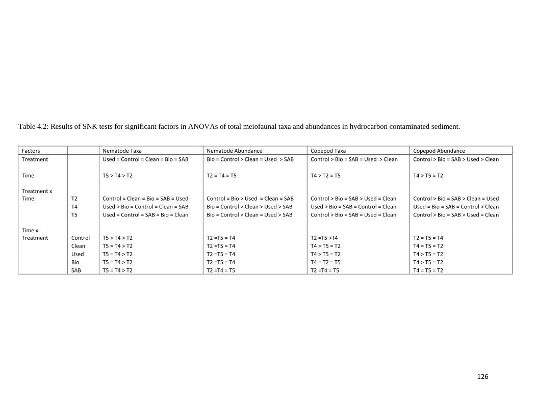
126

Table 4.2: Results of SNK tests for significant factors in ANOVAs of total meiofaunal taxa and abundances in hydrocarbon contaminated sediment.

Factors Nematode Taxa Nematode Abundance Copepod Taxa Copepod Abundance Treatment Used = Control = Clean = Bio = SAB Bio = Control > Clean = Used > SAB Control > Bio = SAB = Used > Clean Control > Bio = SAB > Used > Clean Time T5 > T4 > T2 T2 = T4 = T5 T4 > T2 = T5 T4 > T5 = T2 Treatment x Time T2 Control = Clean = Bio = SAB = Used Control = Bio > Used = Clean = SAB Control > Bio = SAB > Used = Clean Control > Bio = SAB > Clean = Used T4 Used > Bio = Control = Clean = SAB Bio = Control > Clean > Used > SAB Used > Bio = SAB = Control = Clean Used = Bio = SAB = Control > Clean T5 Used = Control = SAB = Bio = Clean Bio = Control > Clean = Used > SAB Control > Bio = SAB = Used = Clean Control > Bio = SAB > Used = Clean Time x Treatment Control T5 > T4 > T2 T2 =T5 = T4 T2 =T5 >T4 T2 = T5 = T4 Clean T5 = T4 > T2 T2 =T5 = T4 T4 > T5 = T2 T4 = T5 = T2 Used T5 = T4 > T2 T2 =T5 = T4 T4 > T5 = T2 T4 > T5 = T2 Bio T5 = T4 > T2 T2 =T5 = T4 T4 = T2 = T5 T4 > T5 = T2 SAB T5 = T4 > T2 T2 =T4 = T5 T2 =T4 = T5 T4 = T5 = T2

127

4.3.4 Multivariate analysis of assemblages

Multivariate analysis of assemblage composition revealed significant differences between

treatments at all times. The nMDS ordination of all 120 samples in the hydrocarbon

experiment showed distinct separation of treatments in the meiofaunal communities at

T2, T4 and T5 (Figure 4.5a). All treatments were significantly different and can be seen

to form independent groups except Control and Biodegradable, where there was some

overlap during T2 and T4 (Figure 4.5b). At T5, all treatments showed independent groups

(Figure 4.5b). Results showed the variation within treatments was less than the variation

between treatments. This is supported by one way ANOSIM analysis in Table 4.3. It is

clear that each treatment elicited a different response in the meiofaunal communities, as

evidenced by their clear separation, but in different directions from the Control treatment

in each nMDS (Figure 4.5b).

A one-way ANOSIM of the four treatments groups against the Control treatment

indicated significant differences (p > 0.1) for all pairwise comparisons, with a range of R-

values indicating differing degrees of discrimination (Table 4.3). Pairwise comparisons of

Control and Biodegradable treatment produced the smallest R value during all times (T2,

T4 and T5) indicating that these two treatments had the most similar composition of

meiofaunal communities.

128

Figure 4.5a: nMDS representing the meiofaunal community, nematodes only and

copepods only at all time (T2, T4, and T5) based on square root transformed abundances

and Bray-Curtis similarities.

TreatmentControlClean LubeUsed LubeBiodegradableSAB

T2

T2

T2

T2

T2T2

T2T2

T2T2

T2

T2T2

T2

T2T2

T2

T2

T2

T2

T2T2T2

T2

T2

T2

T2

T2

T2

T2T2

T2

T2

T2

T2T2

T2T2

T2

T2T4T4

T4 T4T4

T4

T4T4

T4

T4

T4

T4

T4 T4

T4

T4

T4T4

T4

T4

T4T4

T4

T4T4T4 T4

T4T4

T4

T4

T4

T4

T4T4

T4

T4T4

T4

T4

T5T5T5

T5

T5

T5

T5T5

T5

T5

T5T5

T5T5T5

T5

T5

T5

T5

T5

T5

T5T5

T5

T5

T5

T5

T5

T5

T5

T5

T5T5

T5T5

T5

T5 T5T5

T5

2D Stress: 0.21


T2

T2

T2

T2

T2T2

T2T2

T2T2

T2

T2T2T2

T2T2

T2

T2

T2

T2

T2T2

T2T2

T2

T2

T2

T2

T2

T2T2

T2

T2

T2

T2T2

T2 T2

T2

T2

T4T4

T4 T4

T4

T4

T4T4

T4

T4

T4

T4

T4 T4

T4

T4

T4T4

T4T4

T4

T4

T4

T4T4

T4T4T4

T4

T4

T4T4

T4

T4T4

T4

T4

T4

T4T4

T5T5T5

T5

T5T5T5T5

T5

T5

T5

T5

T5T5

T5

T5

T5T5

T5T5

T5 T5T5

T5

T5

T5

T5

T5

T5

T5

T5T5

T5

T5

T5

T5

T5T5T5 T5

2D Stress: 0.19


T2

T2

T2

T2

T2

T2

T2

T2

T2

T2

T2

T2

T2

T2

T2

T2

T2

T2

T2

T2

T2

T2

T2

T2

T2

T2

T2

T2

T2

T2

T2

T2T2

T2

T2

T2T2

T2T2

T2T4

T4

T4

T4

T4

T4

T4

T4

T4

T4

T4

T4

T4

T4

T4

T4

T4

T4

T4

T4

T4 T4

T4T4

T4

T4

T4

T4

T4

T4

T4

T4

T4

T4

T4

T4

T4

T4

T4

T4

T5

T5

T5

T5

T5

T5

T5

T5

T5

T5

T5

T5

T5

T5

T5

T5

T5

T5

T5

T5

T5

T5

T5

T5

T5

T5

T5

T5

T5

T5

T5

T5T5

T5

T5

T5T5

T5T5

T5

2D Stress: 0.29

meiofaunal

nematodes

copepods

129

Figure 4.5b: nMDS representing the meiofaunal community, nematodes only and copepods only at T2 (56 weeks), T4 (104 weeks)

and T5 (260 weeks). Based on square root transformed abundances and Bray-Curtis similarities.


2D Stress: 0.15 2D Stress: 0.14 2D Stress: 0.26



T2

T4

T5

meiofauna nematodes copepods

130

Table 4.3: ANOSIM shows comparison of meiofaunal community structure between the

Control and the treatments at all time interval.

T2, Global R= 0.869, P=0.1

Groups R Statistic Significance Level %

Possible Permutations

Actual Permutations

Number >=Observed

Control, Clean Lube 0.795 0.1 6435 999 0 Control, Used Lube 0.757 0.1 6435 999 0 Control, Biodegradable 0.655 0.1 6435 999 0 Control, SAB 0.871 0.1 6435 999 0 T4 Global R= 0.893, P=0.1



Actual Permutations

Number >=Observed

Control, Clean Lube 0.926 0.1 6435 999 0 Control, Used Lube 0.955 0.1 6435 999 0 Control, Biodegradable 0.357 0.1 6435 999 0 Control, SAB 0.97 0.1 6435 999 0 T5 Global R=0.983, P=0.1



Actual Permutations

Number >=Observed

Control, Clean Lube 1 0.1 6435 999 0 Control, Used Lube 0.984 0.1 6435 999 0 Control, Biodegradable 0.984 0.1 6435 999 0 Control, SAB 1 0.1 6435 999 0

131

4.3.5 Interactions of different Treatments and Times

PERMANOVA results showed significant effects of treatments, time, and an interaction

between treatment and time (PERMANOVA, P < 0.001; Table 4.4). The treatments were

all significantly different to each other at all times and the interaction related mainly to

the size of the differences and relationships among hydrocarbon treatments. Importantly,

the Control maintained significant differences with treatments at all times, though the

size of the effect varied. The Control showed the least degree of change between all time

comparisons, excluding the Used oil treatment which changed the least between T4 and

T5 (Table 4.5b). The Control has the highest percentage of similarity (63.5%) between

times (Table 4.5b).

Table 4.6a and 4.6b show the percentage similarity (from PERMANOVA) breakdown of

the interaction term between treatment and time. Among the treatments, Control and

Biodegradable were the most similar over time (Table 4.6b). All treatments become less

variable over time (Table 4.6b). At all times, the Biodegradable is the most similar to

Control but at the end of experiment, it was more different to the Control than at T4

(Figure 4.6a).

SAB lubricant initially had the largest effect but by T5 all treatments were of

approximately the same magnitude of difference from the Control (Table 4.6b and Figure

4.6b).

132

Table 4.4: PERMANOVA two-factors results.

Source df Pseudo-F P(perm) Unique perms

Treatment 4 16.69 0.0001 9871 Time 2 44.142 0.0001 9909 Treatment x Time 8 10.142 0.0001 9805 Residual 105 Total 119 Estimates of components of variation Source Estimate Square root S(Treatment) 16.87 15.80 S(Time) 27.83 20.29 S(Treatment x Time) 29.49 20.88 V(Residual) 25.81 19.54

Table 4.5a: Pairwise test of Time within Treatment.

Groups Control Clean Used Biodegradable SAB t P t P t P t P t P T2, T4 3.1768 0.0001 3.6605 0.0002 4.1823 0.0001 4.1403 0.0002 4.0893 0.0004 T2, T5 2.8090 0.0002 5.6411 0.0003 4.4828 0.0003 4.5433 0.0001 4.9671 0.0002 T4, T5 3.4956 0.0001 4.4435 0.0004 2.4704 0.0004 3.6477 0.0002 4.6212 0.0001

Table 4.5b: PERMANOVA interaction treatment and time (Times within Treatment).

Percentage of similarity between times.

Control Clean Used Biodegradable SAB T2, T4 58.9 53.7 48.2 50.4 51.0 T2, T5 63.5 41.7 44.7 44.7 42.7 T4, T5 61.0 52.6 66.7 59.9 56.4

133

Table 4.6a: Pairwise test of treatment vs control within level T2, T4, and T5 of factor 'Time'.

Groups T2 T4 T5 t P t P t P Control, Clean Lube 2.9709 0.0002 2.8200 0.0004 5.0203 0.0001 Control, Used Lube 2.6703 0.0002 3.0632 0.0001 3.5203 0.0005 Control, Biodegradable 2.3929 0.0005 1.6227 0.0006 3.1465 0.0001 Control, SAB 3.0125 0.0002 3.2198 0.0002 4.4128 0.0001

Table 4.6b: PERMANOVA interaction treatment and time (Treatment within Times).

Percentage of similarity between treatment T2 T4 T5 Control vs Clean 58.9 62.4 52.9 Control vs Used 58.4 62.8 60.5 Control vs Biodegradable 60.8 72.6 63.2 Control vs SAB 55.5 63.8 56.7 Percentage of similarity within treatment T2 T4 T5 Control 70.7 73.7 76.4 Clean 71.1 71.6 77.1 Used 67.6 74.7 73.6 Biodegradable 67.8 76.5 73.8 SAB 67.2 77.6 76.5

134

Figure 4.6a: Results show the percentage similarity between treatment times in the

interaction of treatment and time.

Figure 4.6b: Results show the percentage similarity within times in the interaction of

treatment and time.

50

55

60

65

70

75

T2 T4 T5

Percentage of similarity between treatment

Control vs Clean

Control vs Used

Control vs Biodegradable

Control vs SAB

65

67

69

71

73

75

77

79

T2 T4 T5

Percentage of similarity within times

Control

Clean

Used

Biodegradable

SAB

135

Similarity percentage analysis (SIMPER) was used to determine the taxa contributing to

the observed difference between and within treatments. The results of the SIMPER

analyses are shown in Table 4.7, 4.8 and 4.9. Several taxa contributed strongly to

differences between treatments at all times, including Daptonema, Dichromadora,

Neochromadora, Paracanthonchus, Paramesonchium, Halalaimus, Linhomoeus and

Monhystera. Nematodes contributed the most to the dissimilarity between treatments and

times but harpacticoid copepods contributed most to the similarity within treatments and

times.

Compared to spatial study in Chapter 2, the control treatments in the hydrocarbon

experiment have a greater number of taxa (65 out of 70) than the spatial study (O’Brien

Bay-1 and O’Brien Bay-5) which is 55 taxa out of 70 (Figure 4.7). Five taxa,

Bolbolaimus, Desmorella, Ancorabolidae, Dactyloposiidae and Romatidae were not

found in the control treatments of hydrocarbon experiment.

Differences between the Control and the treatments were due to a range of different fauna

being present at different times, with some contrasting relationships between each of the

hydrocarbon treatments and the Control. One similarity between the Control and the

treatments was the reduction in the abundance of many taxa from T2 to T5. For some

taxa, a higher abundance was observed at T2 (Figure 4.8). For example, at T2 the

abundance of Neochromadora in the Used and Biodegradable oil treatments was greater

than in the Control, but was lower than the control in the Clean and SAB treatments.

136

Neochromadora was also clearly an opportunistic early colonizer with initially large

abundances that were reduced in all treatments and Control by T4 and T5. Used lubricant

treatment was characterized by the high occurrence of Neochromadora and

Dichromadora, which were also found in Biodegradable treatments at T2. The major

difference between these two treatments was the absence of Halalaimus at T4 and T5 in

Biodegradable and Linhomoeus at T2 in Used treatments.

In the Clean oil treatments, Daptonema and Monhystera was the earliest opportunistic

taxa at T2, this taxa however decreased by T4, whereas Paramesonchium and

Linhomoeus increased in abundance by T5. The Clean oil treatments treatment showed a

resemblance to the Control in the abundance of Neochromadora and Paracanthonchus at

T5. Low values were obtained for both taxa.

Some hydrocarbons initially acted as a stimulus for recruitment, for example

Paracanthonchus had low abundances in all treatments at T2 except for the SAB

treatment, which had high abundances in the SAB treatment, but there was less difference

between treatments and Control by T4 and T5. Halaimus was initially present in all

treatments but in the SAB and biodegradable treatments it was absent at T4 and T5.

BVSTEP procedures were conducted to determine the best subsets of variables (taxa) that

could “best” match that of the treatments data, i.e., could explain the most variation in

137

similarity or dissimilarity between treatments with respect to meiofaunal communities. A

group of 16 taxa, from a total of 65 (Chromadora, Chromadorella, Draconema,

Halalaimus, Leptolaimus, Monhystera, Neochromadora, Southerneilla, Theristus,

Trefusia, Vasostoma, Ameridae, Cletodidae, Idyanthidae, Pseudotachidiidae and

Tachididae) were the best subset that could explain most variation in the meiofaunal

composition pattern (Spearman correlation coefficient ρ = 0.952, P < 0.001). Figure 4.9

shows the mean abundances of these taxa. Halalaimus, Monhystera and Neochromadora

were among the most distinctive taxa in terms of response to the treatments.

138

Table 4.7: Taxa responsible for difference between hydrocarbon treatments in T2 based on SIMPER analysis of square-root transformed data.

T2 Control (78.51) Clean Lube (73.09) Used Lube (72.33) Biodegradable (74.83) SAB (71.02)

Taxa Av.Abund

Contrib%

Av.Abund

Contrib%

Av.Abund

Contrib%

Av.Abund

Contrib%

Av.Abund

Contrib%

Dichromadora 5.61 6.98 5.75 11.24 5.65 9.55 3.51 5.20 Neochromadora 5.28 6.22 7.34 13.48 8.12 13.51 Monhystera 4.53 5.16 6.80 12.36 4.72 6.68 2.49 3.31 Daptonema 3.85 4.44 5.54 9.91 3.04 5.21 Chromadorita 2.86 3.85 2.51 4.60 2.42 3.70 3.06 5.00 Ascolaimus 2.70 3.44 Chromadorina 2.23 2.98 2.69 4.41 2.45 4.63 Paracanthonchus 2.22 2.95 8.30 14.18 Halalaimus 3.04 2.57 4.21 6.48 5.00 8.89 Odonthopora 2.33 2.54 2.54 4.22 Chromadorella 1.95 2.51 3.79 7.38 Linhomoeus 1.82 2.33 4.48 6.91 Metalinhomoeus 1.86 2.31 3.07 5.03 Laophontidae 1.72 2.31 Sphaerolaimus 3.03 5.25 2.66 5.24 Chromadora 2.67 4.33 Theristus 2.57 4.28 Gammanema 3.11 4.63 Promonhystera 2.40 3.84 Spirobolbolaimus 2.41 3.40 Paralinhomoeus 1.82 2.92 3.23 5.45 Leptolaimus 2.35 3.71 Total Taxa : Accumulative % 14 50.6 8 51.23 7 53.26 9 51.77 8 52.66

139


T4 Control (79.23) Clean Lube (78.52) Used Lube (79.72) Biodegradable (81.02) SAB (83.65) Taxa Av.Abund Contrib% Av.Abund Contrib% Av.Abund Contrib% Av.Abund Contrib% Av.Abund Contrib% Dichromadora 4.67 6.07 4.91 6.4 2.07 2.25 4.7 5.53 2.39 3.01 Monhystera 4.47 5.46 4.03 5.1 4.72 5.52 3.47 4.12 Daptonema 3.6 4.78 2.77 3.67 2.69 3.17 5.06 6.44 Paralinhomoeus 3.89 4.67 4.29 5.83 4.72 5.94 Paramesonchium 3.92 4.61 3.31 3.51 4.13 4.87 Molgolaimus 3.69 4.53 3.54 3.97 2.08 2.48 Chromadorita 3.19 4.05 3.5 4.72 2.55 3.01 Leptolaimus 3.38 3.89 3.18 4.22 4.34 4.55 5.54 7.05 Desmolaimus 3.2 3.85 3.28 4.45 2.83 3.23 Linhomoeus 2.62 3.06 3.21 3.54 3.4 4.18 3.52 4.32 Sabatiera 2.29 3.05 Chromadorina 2.28 2.67 3.84 4.99 2.44 2.62 3.09 3.3 Halalaimus 3.39 4.52 Gammanema 2.88 3.87 Sphaerolaimus 2.23 2.85 Ascolaimus 2.75 2.86 Paramonhystera 2.68 2.73 2.8 3.54 2.8 3.1 Trefusia 2.4 2.64 Desmodora 2.47 2.62 2.31 2.89 Neochromadora 2.38 2.61 Chromadorella 2.49 2.47 Chromadora 2.43 2.44 Odonthopora 2.18 2.34 Rhabdocoma 2.26 2.3 2.1 2.51 Paracanthonchus 2.21 2.27 2.2 2.69 2.8 3.48 Wieseria 2.19 2.26 3.52 4.49 Acanthonchus 2.11 2.07 Megadesmolaimus 2.84 3.35 Metalinhomoeus 2.54 2.94 2.88 3.24 Theristus 3.88 4.86 Total Taxa : Accumulative % 12 50.68 11 50.63 18 51.61 13 50.53 13 51.16

140


T5 Control (82.51) Clean Lube (80.67) Used Lube (79.22) Biodegradable (79.46) SAB (82.37) Taxa Av.Abund Contrib% Av.Abund Contrib% Av.Abund Contrib% Av.Abund Contrib% Av.Abund Contrib% Halalaimus 5.26 5.87 Paracanthonchus 4.03 4.49 3.77 4.52 2.4 2.62 Dichromadora 3.53 4.08 Paralinhomoeus 3.5 3.89 4.6 6.68 4.26 5.41 Paramesonchium 3.13 3.18 4.13 5.69 2.64 2.98 4.04 5.26 Megadesmolaimus 2.67 3.09 2.85 3.39 Leptolaimus 2.67 3.03 4.2 4.56 3.86 4.29 4.25 5.31 Chromadora 2.69 3.01 Paramonhystera 2.68 2.82 2.61 2.94 2.43 2.99 2.88 3.24 Linhomoeus 2.67 2.8 4.25 6.3 2.89 3.33 3.12 3.56 Draconema 2.44 2.65 3.93 5.55 3.17 3.96 2.23 2.87 Daptonema 2.48 2.54 2.68 3.08 Monhystera 2.33 2.52 2.25 2.59 2.77 3.39 Microlaimus 2.29 2.38 Chromadorina 2.08 2.3 3.46 4.99 2.38 2.87 2.91 2.95 Neochromadora 2.02 2.23 Pirrickia 5.04 7.32 3.38 4.28 Desmolaimus 4.13 5.98 2.66 3.29 4.72 5.9 Ixonema 3.56 4.96 2.77 3.27 3.17 3.68 Metalinhomoeus 2.9 3.91 Trefusia 3.08 4.02 Theristus 3.13 3.74 Chromadorita 2.87 3.3 2.21 2.59 Desmodora 2.59 3.2 Wieseria 2.68 2.86 Aponema 2.6 2.84 Promonhystera 2.21 2.83 2.37 2.77 Odonthopora 2.18 2.75 2 2.59 Chromadorella 2.56 2.74 Vasostoma 2.46 2.7 3.62 4.61 Acanthonchus 2.33 2.69 Southerneilla 2.25 2.59 3.47 4.13 Spirobolbolaimus 3.6 4.49

Total Taxa : Accumulative % 16 50.89 9 51.38 16 50.34 14 51.51 14 52.13

141

Figure 4.7: Histogram of comparison abundances and taxa between two different studies (control locations in spatial study vs control

treatments in hydrocarbon).

0

100

200

300

400

500

Acan

thon

chus

Aegi

alol

aim

usAp

onem

aAs

cola

imus

Bolb

olai

mus

Chro

mad

ora

Chro

mad

orel

laCh

rom

ador

ina

Chro

mad

orita

Dap

tone

ma

Des

mod

ora

Des

mor

ella

Des

mol

aim

usD

ichr

omad

ora

Dra

cone

ma

Gam

man

ema

Hal

alai

mus

Ixon

ema

Lept

olai

mus

Linh

omoe

usM

egad

esm

olai

mus

Met

alin

hom

oeus

Mic

rola

imus

Mol

gola

imus

Mon

hyst

era

Neo

chro

mad

ora

Odo

ntho

pora

Para

cant

honc

hus

Para

linho

moe

sPa

ram

eson

chiu

mPi

rric

kia

Para

mon

hyst

era

Prom

onhy

ster

aRh

abdo

com

aSa

bati

era

Sout

hern

eilla

Spha

erol

aim

usSp

irob

olbo

laim

usTh

eris

tus

Tref

usia

Vaso

stom

aW

iese

ria

Aegi

sthi

dae

Amei

rida

eAn

cora

bolid

ae

Arge

stid

aeCa

ntho

cam

ptid

ae

Canu

ellid

aeCl

etod

idae

D

iosa

ccid

aeD

acty

lopu

siida

eEc

tino

som

atid

aeH

arpa

ctic

idae

Hun

tem

anni

idae

Idya

nthi

dae

Laop

hont

idae

Mir

aciid

aeN

eobr

adyi

dae

Para

mei

rops

isPa

ram

esoc

hrid

aePa

rana

nnop

idae

Para

sten

helii

dae

Pseu

dota

chid

iidae

Rhiz

othr

icid

aeRo

met

idae

Ta

chid

idae

Tega

sida

eTh

ales

trid

aeTi

sbid

aeZo

sim

idae

mea

n ab

unda

nce

Spatial-control locations (OB1 & OB5)Hydrocarbon- control treatments

142

Figure 4.8: Mean abundances of important taxa (summarized from SIMPER results)

at each treatment and time.

0.005.00

10.0015.0020.0025.0030.0035.00

T2 T4 T5

Ave

rage

abun

danc

ea) Daptonema

Control

Clean

Used

Biodegradable

SAB

0.00

10.00

20.00

30.00

40.00

50.00

T2 T4 T5

Ave

rage

Abu

ndan

ce

b) Dichromadora

Control

Clean

Used

Biodegradable

SAB

0.0010.0020.0030.0040.0050.0060.0070.0080.00

T2 T4 T5

Ave

rage

abun

danc

e

c) Neochromadora

Control

Clean

Used

Biodegradable

SAB

0.0010.0020.0030.0040.0050.0060.0070.0080.00

T2 T4 T5

Ave

rage

abun

danc

e

d) Paracanthonchus

Control

Clean

Used

Biodegradable

SAB

0.00

5.00

10.00

15.00

20.00

25.00

T2 T4 T5

Ave

rage

abun

danc

e

e) Paramesonchium

Control

Clean

Used

Biodegradable

SAB

0.005.00

10.0015.0020.0025.0030.0035.00

T2 T4 T5

Ave

rage

abun

danc

e

f) Halalaimus

Control

Clean

Used

Biodegradable

SAB

0.00

5.00

10.00

15.00

20.00

25.00

30.00

T2 T4 T5

Ave

rage

abun

danc

e

g) Linhomoes

Control

Clean

Used

Biodegradable

SAB

0.00

10.00

20.00

30.00

40.00

50.00

60.00

T2 T4 T5

Ave

rage

abun

danc

e

h) Monhystera

Control

Clean

Used

Biodegradable

SAB

143

Figure 4.9: Results from BVSTEP analyses showing 16 taxa of the best subset that

explained the most variation in meiofaunal composition among treatments (Spearman

correlation coefficient ρ = 0.952, P < 0.001).

0

20

40

60

80Control

T2

T4

T5

0

20

40

60

80Clean

T2

T4

T5

0

20

40

60

80Used

T2

T4

T5

0

20

40

60

80Biodegradable

T2

T4

T5

0

20

40

60

80

Chr

omad

ora

Chr

omad

orel

la

Dra

cone

ma

Lep

tola

imus

Sout

hern

eilla

The

rist

us

Tre

fusi

a

Vas

osto

ma

Am

erid

ae

Cle

todi

dae

Idya

nthi

dae

Pseu

dota

chid

iidae

Rhi

zoth

rici

dae

Hal

alai

mus

Mon

hyst

era

Neo

chro

mad

ora

SAB

T2

T4

T5

144

4.4 Discussion

Several studies have revealed the sensitivity of meiofauna to various kinds of human

activities (Veiga et al., 2009, Beier and Traunspurger, 2001, Bejarano et al., 2006,

Moreno et al., 2008) and concluded that meiofauna are good biological indicators for

environment impact assessments (Sutherland et al., 2007, Kennedy and Jacoby, 1999,

Gyedu-Ababio et al., 1999). The general finding of the above studies is that

anthropogenic disturbance and hydrocarbon pollution can alter meiofaunal

abundance, species composition, biomass, and diversity. For many individual taxa

these alterations are however ambiguous, where the mean values could have either a

positive or negative relationship with the impacted and control locations.

Furthermore, the impacts are also time dependent and the effects of short-term

exposure differs from long term-exposure.

This study is part of a large interdisciplinary project examining the long-term

degradation rates of synthetic lubricants and fuel in Antarctic marine sediments and

the effects of such lubricants on recruiting infauna (Thompson et al. (2006, 2007),

benthic diatom (Cunningham et al., 2003) and microbial communities (Powell et al.,

2005b, Powell et al., 2007). This study presents the long term changes in meiofaunal

assemblages recruiting to the hydrocarbon contaminated and control sediments from

56 to 260 weeks after deployment. Differences in benthic assemblages between

contaminated and control sediments were significant after 56 weeks, with more

obvious differences after 260 weeks (Figure 4.7). This indicates that after a

hydrocarbon spill, whether fuel such as SAB diesel or oil, impacts to benthic

145

communities occur quickly and may persist and become more obvious and severe

after a longer period. There was no evidence of recovery even after five years

suggesting that recovery to pre-spill communities may take a decade or longer.

4.4.1 Loss of oils from sediment

Naturally occurring hydrocarbons in Antarctic marine sediments have been previously

reported in a range from 0.1 to 9.3 mg TPH kg -1 (Cripps and Priddle, 1991).

However, values up to 289 mg TPH kg -1 were recorded here in the Control at T3.

Initially values in control sediment were at background levels. All sediment for

experimentation was collected from unpolluted O’Brien Bay. The increase in TPH in

control sediments may be due to resuspension of sediment from nearby contaminated

trays. Alternatively it may be due to microbial activity in the sediments.

In this study, large decreases in TPH values were observed by 260 weeks after

deployment. A significant loss of 53 to 87% of all oils was observed in the top 1 cm.

Biodegradable lubricant oil recorded a loss of up to 87% after 260 weeks. Loss of

hydrocarbons from sediment occurs through several processes, especially dilution,

dissolution and biodegradation (Powell et al., 2007). A decrease in the TPH values

indicates an overall loss of hydrocarbons but the effect on meiofaunal communities is

still strong. This effect was clearly seen in the MDS pattern for T5 (Figure 4.5b) as

each treatment was distinctively grouped. This may be because compounds contained

146

within the hydrocarbons, which may also be highly toxic, still remain and may be

more difficult to degrade or change over time.

4.4.2 Effects of hydrocarbon contaminated sediment on meiofauna

The effects of hydrocarbons on the meiofaunal assemblages differed between

treatments and exposure time. The Clean, Used, and SAB treatments initially had a

greater effect than the Biodegradable oil. A significant reduction in mean abundance

of meiofauna was observed in those treatments compared to the Control. In contrast,

the Biodegradable oil did not have a significant effect on the total abundance of

meiofauna (and thus on the total abundance of nematodes) but did have a significant

effect on the community composition during the study period. Heip et al. (1985) and

Danovaro et al. (1995) observed that high densities of opportunistic nematode species

were present after oil spills, probably as a consequence of the increase in bacterial

density in the sediments. These bacteria have been found to be an important food

source for nematodes after an oil spill (Heip, 1985). This observation is consistent

with the findings of Powell et al (unpublished data) on Antarctic benthic microbial

communities at T1 (five weeks). In their study total bacterial cell numbers increased

in all hydrocarbon treatments compared to the Control. In the SAB and Biodegradable

oil treatments an increase in hydrocarbon degrading bacteria was observed after five

weeks. The Biodegradable oil did not have strong effect on the microbial community

after 56 weeks of exposure but it became more different to the Control after 104 and

260 weeks (Powel, unpublished data). In this experiment the abundance of nematodes

did not increase in any of the hydrocarbon treatments, but decreased in most, except

147

the biodegradable treatment which was not different to the control in terms of

abundance. These findings are in contrast to other work which has demonstrated an

increase in nematode abundance in response to hydrocarbon contamination (Heip et

al., 1985). However, the meiofaunal communities were not sampled at five weeks and

it is possible they may have increased initially and this response would have gone

undetected. In contrast, the abundance of copepods was lower in the Biodegradable

treatment than in the Control at 56 weeks and 260 weeks. Although similar

conclusions have been reached by many studies whereby meiofaunal communities are

a good indicator of environmental change, many of these studies have yielded

different results. Some studies showed that hydrocarbon contamination may influence

whole groups of meiobenthic taxa negatively or positively. Generally results obtained

from field survey experiments constantly showed acute toxicity effects (reduction in

taxa) on meiofauna community immediately after an oil spill (Veiga et al., 2009,

Danovaro et al., 1995). While, in laboratory or mesocosm experiment, variability in

responses to contamination may occur where increases or reduction in several

meiofauna taxa were observed only at certain stages (by time). This trend was

observed in this current experiment, whereby indicating a colonization process.

Similarly, Fleeger and Chandler (1983) found that several taxa of meiofauna did

respond positively to oil application after 90 days of oil introduction and significantly

decreases after 150 days. A negative response which is similar to the Casey

experiment, was found in a mesocosm experiment conducted by Beyrem et al (2009),

which showed a significant decrease in total nematode abundance (I), species richness

(d) and number of species (S) after five days exposure. Similar results were found in a

study by Frithsen et al. (1985), most metazoan meiofaunal groups showed decreased

abundance in the presence of high dosage of oil (average 190 ppb in water column) in

148

168 days. This variability in responses of meiofauna to oil contamination may be

caused by difference in experimental setup and exposure duration.

Fleeger and Chandler (1983) suggested that increase in meiofauna were due to

increased bacterial production in oiled sediments, and subsequent heightened copepod

grazing. In this study, the only increase in meiofaunal abundance was for copepods in

the SAB treatment. However, the SAB diesel treatments showed the most significant

decreases in nematode abundances in comparison to other treatments after five years.

Powell (2005a) reported that the microbial community in the SAB treatment had

changed the most after five weeks and was significantly different from the Control.

They suggested that the increase in bacterial numbers was due to the input of carbon

from the degradation of the SAB. However, after 260 weeks, no significant

differences were observed. They concluded that the hydrocarbon degrading bacteria

continued to dominate the community after five years (Powel, unpublished data).

Results of this study indicate that nematodes are generally perhaps more tolerant to

hydrocarbon pollution than copepods but that nematodes still clearly respond to

hydrocarbon pollution. Similar observations have been reported in other studies

(Veiga et al., 2009). High abundances of nematodes were found in most treatment

groups. It is well established that nematodes are highly tolerant of stressed

environmental conditions, while copepods are more sensitive to disturbance (Mirto et

al., 2002). Consequently, the copepod community may be more suitable for short term

monitoring due to their sensitivity to pollution. In this study the copepods were

generally more sensitive to hydrocarbon contaminated sediments, having a lower

149

abundance in all treatment groups at 56 and 260 weeks. Similar results were found in

Fleeger and Chandler (1983) and Frithsen et al. (1985). These findings are in contrast

to those of Thompson et al. (2007) who reported that copepods (> 300 µm) dominated

the infaunal assemblages in the contaminated and Control sediments at five and 56

weeks and their recruitment was largely unaffected by the presence of lubricants, but

they did not examine the SAB treatment, nor did they identify the copepods beyond

this taxonomic level. They reported that the short-term response (five weeks), T1

(ANOVA treatment F3,12 = 3.96, p = 0.036) the abundance in the control was greater

than in the oil treatments. After 56 weeks (T2), there were no significant effects. They

concluded that the copepods were opportunistic because of their potential for rapid

reproduction, which allowed them to dominate the initial stages of faunal succession

after a disturbance. An increase in copepod abundance in most of the hydrocarbon

treatments at 104 weeks suggests that copepod assemblages may have been

responding to some other external factor, as by 260 weeks they all had lower

abundances than the control again.

In the Control treatment, some taxa showed a trend of decreasing abundances from 56

to 260 weeks. For example, Dichromadora and Neochromadora were dominant at 56

weeks. These taxa were then replaced as the dominant taxa in the control by

Halalaimus after 260 weeks. Halalaimus could be considered as an intolerant to oil

contamination since it was eliminated or significantly reduced after 260 weeks of

exposure to Clean, Used, Biodegradable and SAB hydrocarbons. In the Biodegradable

and Used treatments, Neochromadora was initially dominant, confirming its status as

opportunistic taxa, but by 104 and 260 weeks it had drastically declined in all

treatments where it was initially abundant. Other taxa generally increased in

150

abundance from 56 to 104 and 260 weeks, including Paramesonchium, Draconema

and Leptolaimus. In the Biodegradable treatment, Daptonema increased marginally

from 56 to 260 weeks but decreases occurred in the other treatments suggesting it may

be tolerance to only Biodegradable oil. Beyrem et al. (2009) also reported that

Daptonema was intolerant to oil contamination, since it was eliminated after five

weeks when exposed to hydrocarbons. In other studies, after a long exposure to oil,

the sediment hydrocarbon levels decreased, enabling the benthic communities to

recover to their normal density and diversity values (Wormald, 1976, Giere, 1979,

Bodin, 1988). This was not observed here after the five years of this experiment and

strong and obvious effects were still apparent. Similarly, the Clean, Used and SAB

showed changes in abundance of many taxa from 56 to 260 weeks. These changes

suggest that exposure to long term hydrocarbon pollution may cause changes in

community composition, with only tolerant taxa being able to survive. Monhystera

has been characterized as an opportunistic coloniser genus due to its ability to live in

polluted areas (Gyedu-Ababio et al., 1999), but here its abundance generally declined

over time in all hydrocarbon treatments where it was initially abundant, showing

opportunistic traits. Huge decrease was observed in Clean and Used lubricant

treatment. Used lubricants contain metals and additional polycyclic aromatic

hydrocarbons that are introduced via engine operation and oil combustion (Thompson

et al., 2007). Thompson (2006) suggested that Used lubricant could be biologically

degraded as fast as their unused (Clean lubricant) counterpart, where, the alkyl

naphthalenes, alpha olefins and alkyl diphenylamines behaved similarly in both Used

and Clean treatments. According to Thompson et al. (2007), lubricants contain many

toxic compounds such as diphenylamines, alkyl naphthalenes and other minor phenol

additives that are not readily biodegradable. Such compounds are very toxic to many

151

aquatic organisms such as bioluminescent bacteria (Photobacterium phosphoreum),

amphipods (Gammarus fasciatus) and daphnia (Daphnia magna) (Drzyzga, 2003).

These compounds may remain in sediments after the readily biodegradable fractions

have gone and contribute to long term impacts on meiofaunal communities.

Similarities in abundances of meiofauna were observed between the Control and the

Biodegradable treatments, which also had the most similar meiofaunal community

composition at 56 and 104 weeks. But by 260 weeks, it showed as much difference

from the Control as the other hydrocarbon in terms of whole community patterns.

These results suggest that prolonged exposure to Biodegradable lubricant will not

alter the meiofaunal abundances but will alter community composition. This suggests

that Biodegradable lubricant is initially less harmful but may break down into more

harmful compounds, which create long term impacts. It may be suitable as an

alternative to other oils to minimize the impact of hydrocarbon contamination in

Antarctica, as meiofaunal abundances were not affected.

Comparison with Casey macrofaunal assemblage can only be done at T2 in a study by

Thompson et al (2007). For example, they found significant reductions in the

abundance of many infaunal species in hydrocarbon treatments including cumaceans,

amphipods, tanaids and polychaetes after T2 (56 weeks). However, they noted that

Evenness (J′) did not differ significantly across all treatments after 56 weeks; Control

sediments had a significantly greater Evenness than the Biodegradable treatment, but

not the Clean or Used treatments. In contrast, significant differences were observed

between all treatments in the meiofauna experiment at T2. Thompson et al (2007) also

152

concluded that the Biodegradable oil possess the same effect on recruitment of

macrofauna as the other conventional lubricants. This is in contrast with meiofauna

whereby Biodegradable showed similar responses to the Control treatment. In a

relevant study at Casey it was noted that, sediments which were artificially

contaminated by hydrocarbons had greater effects on recruitment than those with

sediments which were treated with a complex of metals (Stark et al., 2003b).

However, in general, the disturbed locations (sites near to Casey Station) had a lower

diversity of soft sediment macrofaunal assemblages, but often recorded higher

abundances of individuals in hydrocarbon treated sediment by comparison to control

(Stark et al., 2003a).While, in undisturbed location such as O’Brien Bay less effect of

the hydrocarbon contamination were observed (Stark et al., 2003b).

This experiment was designed to investigate both short (56 weeks) and long-term

(260 weeks) effects of diesel fuel and synthetic lubricants on meiofaunal

communities. It was observed that each treatment has different effects on meiofaunal

communities. Results from this study confirm that changes in nematode assemblages

are ideal for long term pollution monitoring as they displayed clear responses to

hydrocarbon pollution, both in terms of taxon abundance and community

composition. In conclusion, the effects of lubricant contamination on Antarctic

meiofauna may be measurable for at least five years after a spill.

153

5.0: GENERAL DISCUSSION

The Antarctic ecosystem is considered one of the world’s most pristine environments,

however, the integrity of the environment is threatened by contamination resulting

from human activities. The presence of research stations on the Antarctic continent

has contributed to the contamination of coastal waters and ecosystems. To date there

have been few studies of composition, distribution, and diversity of Antarctic free-

living nematode and harpacticoid copepod communities at the species level. This

study provides the first general picture of the spatial distribution and structure of the

meiofaunal communities and their variability in subtidal coastal waters near Casey

Station, East Antarctica. In this thesis, the impact of human activities at a permanently

manned research station, Casey, was studied by comparing meiofaunal assemblages at

both control and disturbed locations and relating these patterns to sediment

contamination and other environmental variables.

A survey of meiofaunal communities was undertaken to determine the spatial

variation, abundance, and biodiversity of meiofauna at several scales (Chapter 2).

Relationships between spatial patterns of meiofaunal communities and the

environment were examined using environmental data such as grain size, organic

carbon, and sediment metal concentrations (Chapter 3). In addition, the responses of

free-living nematode and harpacticoid copepod communities to hydrocarbon pollution

were investigated in an experiment (Chapter 4).

154

5.1 Summary of findings

The spatial variation of meiofaunal communities at Casey Station was observed

between locations (1000’s of meters), between sites within locations (100’s meters)

and between plots within sites (10’s of meters). The greatest differences were at the

largest scale, between locations, although significant differences in meiofaunal

assemblages were found at each spatial scale measured. There were significant

differences between the meiofauna at all locations but there was also a very

distinctive pattern between control and disturbed locations. Higher abundances of

meiofauna were recorded in control locations (O’Brien Bay and McGrady Cove) than

disturbed locations (Brown Bay and Wilkes).

In this study, statistical analyses revealed that sediment metal contamination showed

significant correlations with patterns of meiofauna distribution and composition. It is

proposed that there is a strong relationship between meiofaunal community structure

and the extent and type of metal contamination of sediments. In addition to the clear

differences between all locations and the potentially strong influence of metals on this

pattern there were also clear patterns in the distribution of specific taxa which related

to these differences. Some taxa were able to be classified as either opportunistic or

sensitive in their relationship to the presence of contamination. For example, the taxa

Halalaimus and Zosimidae were found to be pollutant sensitive, since they were only

present at control locations. This was also found in the hydrocarbon experiment,

where Halalaimus was found to be sensitive to all hydrocarbon treatments. Two taxa,

Promonhystera (nematode) and Paramesochridae (harpaticoid copepod), were only

155

found in the disturbed locations of Brown Bay Inner, Brown Bay Middle and Wilkes

and appear to be tolerant of disturbance and could be considered to be opportunistic

species. While, the genera Paramonhsytera and Theristus, which were found to be

tolerant to metal pollution, were found be important taxa in Brown Bay.

5.2 The composition of meiofaunal assemblages at Casey, Antarctica

A total of 58 different meiofaunal higher taxa were identified from Casey. The

meiofauna assemblage was generally dominated by nematodes (38 genera) and

harpacticoid copepods (20 families). The ratio of nematodes to copepods was

approximately 4:1. This ratio of nematodes to copepods has previously been observed

in other ecosystems, including intertidal mudflats, mangroves, and coastal intertidal

areas (Vanaverbeke et al., 1997b, Moreno et al., 2008, Chinnadurai and Fernando,

2007, Ndaro and Ólafsson, 1999, Delgado et al., 2009). This ratio (Ne/Co) has been

previously used as a tool in biomonitoring programs based on the argument that

nematodes are more pollution tolerant than copepods (Raffaelli and Mason (1981)

However, several studies argued that the index, as proposed, was not universally

applicable to all habitats (Coull et al., 1981, Lambshead, 1984, Lee et al., 2001b).

Peterson et al. (1996) argued that the method could be useful if the differential

response of major (even phylum level) meiofaunal taxa to various pollutant stressors,

such as sediment toxicants and organic loading, were better understood but Lee at al.

(2001b) concluded that the ratio could not be used as a standalone method for

156

biomonitoring purpose especially on high energy open ocean beaches, due to the low

densities of meiofauna and the absence of harpacticoid copepods from the beaches.

Furthermore, the abundance of copepod and nematodes and their response to

contamination may vary in different habitats. Interestingly, a ratio of 4:1 (Nematodes:

Copepods) was consistently observed in both the controlled and disturbed locations at

Casey, (Chapter 2).

The dominant taxa were the nematode genera Monhystera and Daptonema, which

were found at all six locations. The most abundant meiofauna taxa, summed over all

six locations, were Monhystera (11.5%), Daptonema (8%), Neochromadora (6.3%),

Tisbidae (4%), Odonthopora (3.6%), Halalaimus (3.5%), and Chromadorina (3.4%),

all of which are nematodes except for Tisbidae. This composition is similar to other

Antarctica meiofaunal communities. Most of the nematode taxa found in this study

have also been recorded in the southeastern Weddell Sea shelf and slope (200 to 2000

m). These taxa include Monhystera, Daptonema, Sabatiera and Dichromadora

(Vanhove et al., 1999). In the Weddell Abyssal Plain, nematodes dominated the

communities (90%) followed by copepods (5%), with a total of 17 taxa. Similarly,

Lee (2001a) notes that Monhystera was the dominant taxon out of 38 taxa found in a

study of Kapp Norvegia, Weddell Sea. Monhystera is known to have a worldwide

distribution (Alongi and Tietjen, 1990, Gerlach and Schrage, 1971, Vanreusel et al.,

2000, Vanaverbeke et al., 1997a, Vanhove et al., 1999) and has been found

abundantly in both organically enriched and polluted sediments (Lorenzen et al.,

1987, Gyedu-Ababio et al., 1999) and is known as a colonizer genus and is considered

an indicator of pollution (Veiga et al., 2009). The genus Monhystera also has the

highest abundance at the disturbed location of Brown Bay, Casey (Chapter 2).

157

In addition to Monhystera, Daptonema was also found to be abundant at Casey. This

genus, Daptonema, has also been reported as one of the most abundant genera in the

shallower areas (230m) of the deep, Arctic Laptev Sea (Vanaverbeke et al., 1997a).

Tisbidae, a marine benthic copepod, had a high abundance at the Wilkes location.

This family is commonly found between depths of 20-200 m (Seifried, 2004) and is

widely distributed in communities adjacent to the Ross Ice Shelf (Bradford and Wells,

1983), Weddell Sea (Dahms, 1989, Günther et al., 1999, Schunemann et al., 2008)

and the South Orkney Islands (Gee and Fleeger, 2008), Antarctica.

Sabatiera and Daptonema are typically found in organically rich, muddy sediments

(Heip et al., 1990, Schratzberger et al., 2006) and are thought to be well adapted to

disturbed conditions (Vanreusel, 1990). In particular, the genus Sabatieria survives at

low oxygen concentrations and high sulphide concentrations and often persists under

conditions that are unsuitable for most other nematode species (Hendelberg and

Jensen, 1993, Steyaert et al., 1999, Tietjen, 1980). At Casey, Sabatiera was found at

the disturbed location, Brown Bay, but was least abundant at the control location,

O’Brien Bay. In contrast, Daptonema was dominant at McGrady Cove, which had a

high proportion of coarse sand and is the control location in Newcomb Bay.

Daptonema has also been found in a heavily polluted harbour in Ligurian Sea, which

is characterized by silt and muddy sediments (Moreno (2008). It is known that the

sediment type affects meiofauna composition. For example, Doulgeraki et al. (2006)

noted that meiofauna are often more abundant and diverse at sites with coarse

sediments where water circulates more freely, resulting in a better oxygenation of the

substrate, a condition which would also allow a deeper penetration of meiofauna. This

suggests that both the presence of pollution and sediment type contributes to the

158

meiofaunal community composition and distribution. The composition of meiofauna

at Casey is similar to most studies in the Antarctic and other regions and has a similar

relationship to sediment grain size and pollutants.

5.3 The effects of heavy metal and hydrocarbon contamination on meiofaunal

communities

The field survey indicates that Antarctic meiofauna are sensitive to elevated metal

concentrations contributed from both anthropogenic and non-anthropogenic sources

(Chapter 3). Findings from this study not only suggest that heavy metal pollution from

activities at Casey Station reduces meiofaunal abundance but that it may also alter the

composition. In a previous study, it was demonstrated that there were higher

concentrations of some heavy metals in sediment collected from bays adjacent to

Casey Station (Brown Bay and Wilkes) in comparison to control locations which were

situated further away (Cunningham et al., 2005, Stark et al., 2003b). The presence of

these pollutants was correlated with patterns of differences in macrofaunal

assemblages (Stark et al (2003b) in a similar manner to meiofaunal communities.

Anthropogenic contamination of marine sediments was obvious at some disturbed

locations such as Brown Bay. However, Wilkes, a potentially disturbed location, had

metal concentrations and meiofaunal assemblages similar to the control locations. The

Wilkes waste dump site is much older than the Casey site and has not been disturbed

159

recently and also does not have a melt stream running through it. The concentration of

most metals was similar to the controls except for a few, Cd and Zn and to a lesser

degree, Pb and Sn, which were slightly higher. Meiofaunal assemblages at Wilkes

were similar to those of the control sites (O’Brien Bay) in some ways but in other

ways resembled a disturbed location, suggesting that perhaps it was impacted at some

point in its past since human occupation. Wilkes may have recovered from pollution

impacts if they existed in the past, or there may be other unmeasured contaminants

present..

Higher concentrations of heavy metals are typically associated with the fine-grained

fraction of the sediment rather that the coarse-sized fractions (Tam and Wong, 2000),

although this difference becomes less significant when the region becomes more

contaminated. In this current study, Brown Bay, which is the most disturbed location,

had the highest fraction of fine sediment and the highest metal concentrations. While

O’Brien Bay, located well away from the Station, had coarser sediments and much

lower metal concentrations. McGrady Cove, the control location in Newcomb Bay,

also recorded high concentrations of some metals, such as Ag, As, Cd, Ba and Th, and

it also had fairly fine sediments. This suggests that fine sediment could enhance the

effects human impacts in the presence of heavy metals. Wilkes, however, had coarser

sediments more similar to the control sites, which may have influenced the metal

concentrations measured there. Coarse sediments have been found to increase the

toxicity of sediment metals, so that lower concentrations can be as toxic as at sites

with fine grained sediments and higher concentrations (Pesch 1979).

160

Most studies of meiofauna and metal toxicity have been conducted in microcosm

experiments (Mahmoudi et al., 2007, Ellis et al., 2001, Austen and McEvoy, 1997,

Millward and Grant, 2000, Millward et al., 2001, Fichet et al., 1999, Lee et al., 2001b,

Ser, 1991, Beyrem et al., 2007). These laboratory experiments have tended to show

that metals as toxicants have either lethal or sublethal effects, which tend to increase

with increased metal concentrations (Somerfield et al., 1994). A decrease in diversity

is therefore to be expected as a community responds to metal pollution. In our field

study, such a conclusion could not be made since the effects were from a combination

of a number of heavy metals and other interacting environmental factors, however,

changes in the community structure were still observed. Furthermore, nMDS analysis

showed that there was a distinctive pattern of meiofauna between disturbed and

control locations. This is in an agreement with Tietjen (1980), who found that there

was a clear relationship between metal concentrations and decreased nematode

diversity.

Human activities in the Antarctic are heavily dependent on petroleum and synthetic

oil products for transport, power, and heating. Wide ranges of lubricating oils are used

in vehicles and heavy machinery. Given the harsh operating conditions and the

quantity of oil that is used in the Antarctic, there is a significant risk of spills entering

the marine environment. Two different type of hydrocarbons commonly used at Casey

Station (SAB diesel fuel, and a Clean lubricant oil) as well as the same clean lubricant

after use in machinery (Used Lubricant) and a potential alternative to conventional

petroleum based lubricants, a Biodegradable lubricant oil, were examined to

determine their effects on sediment meiofaunal communities. Each of the four

hydrocarbons was found to have a strong effect on the meiofaunal communities at

161

Casey even after five years, when significant biodegradation of the contaminants had

occurred in the top layer of sediment. Duration of contaminant (hydrocarbon)

exposure was shown to be important, as at each sampling time different effects on the

meiofaunal assemblages were observed. For example, the biodegradable oil appeared

to have little effect for the first few years but by five years it had a strong effect on

communities (Chapter 4). The changes demonstrate that exposure to long term

hydrocarbon pollution will cause changes in community composition, where tolerant

taxa are able to survive and dominate assemblages. Results from this study suggest

that changes in nematode assemblages are ideal for long term pollution monitoring as

they displayed some very clear responses to hydrocarbon pollution, particularly in

terms of their abundance.

In polluted areas, a few tolerant or opportunistic taxa will become relatively more

numerous and dominate the community, while less tolerant species will become

increasingly rare or disappear (Moreno et al., 2009, Gyedu-Ababio et al., 1999,

Gyedu-Ababio and Baird, 2006). In this hydrocarbon experiment, changes in species

composition were observed, for example, in all oil treatments, Halalaimus was

present at the early stage of the experiment (T2), however, this taxa become rare (in

Used Oil) and disappeared (in other oils) after prolonged exposure (T5). Taxa such as

Neochromodora were seen as an early colonizing, opportunistic species and was only

abundant at early stages, and was reduced after 260 weeks. Observation of species

elimination was also observed by Mahmoudi et al (2005) in a microcosm experiment,

whereby gradual changes in community structure were revealed, when a quantity of

diesel (ranging from 0.5 to 20 mg diesel kg-1) was administrated. Species such as

162

Chaetonema were eliminated after 90 days and Hypontolaimus colesi and Daptonema

trabeculosum dominated the contaminated sediment.

In a monitoring program after an accidental spill of diesel fuel at Faraday Research

Station, Galindez Island, Antarctica in March 1992, it was observed that there were

high n-alkane and PAH concentrations in the seawater near the station immediately

after the spill but these decreased to local background concentrations within a week

(Cripps and Shears, 1997). The diesel spill had an immediate toxic effect in the

intertidal zone but the fuel dispersed quickly, due to evaporation, dissolution, and

dispersal. However, concentrations in the animals living close to the station never

decreased to the levels found at the uncontaminated control site (Cripps and Shears,

1997). Similarly, results from this thesis showed that while there was a decrease in

TPH after five years, the impacts on the meiofaunal communities were still apparent.

Vincx and Heip (1991) concluded that while there is usually an obvious decrease in

nematode abundance after an oil spill, and after a year, a huge increase in a few

opportunistic species could occur. A similar trend was observed in this study where

the abundance of several taxa decreased or were replaced after being treated with

hydrocarbon for 48 weeks (Chapter 4).

163

5.4 Comparison of meiofauna as a biological indicator with other marine benthic

communities

There are several characteristics that enable meiofaunal communities to be used as

biological indicators. For instance, this community responds rapidly to perturbation,

possesses a close relationship with the sediment matrix and has a short life cycle

(Kennedy and Jacoby, 1999, Moreno et al., 2008). Meiofauna may seem to have more

advantages as indicator species than other benthic invertebrates as they are confined

to the substrate throughout their life cycle. Although having advantages, there are also

several drawbacks of using meiofauna for environmental monitoring (Table 5.1).

Benthic diatoms apparently have similar advantages to the meiofaunal community as

they also have short regeneration times and respond quickly to environmental changes

(Cunningham et al., 2005). Despite this, there is little information on the impact of

petroleum hydrocarbons and metal contamination on benthic marine diatoms.

Cunningham et al. (2003), Cunningham and McMinn (2004) and Cunningham et al.

(2005) showed that benthic diatom communities were affected by both hydrocarbon

and metal contamination at Casey Station. Although responses to pollution may be

different between benthic diatom and meiofaunal communities, both communities are

sensitive to disturbance and anthropogenic pollution.

While the meiofauna have some advantages as indicator species compared to

macrofauna (Table 5.1), studies have shown that some macrofauna are also reliable in

indicating the presence of pollution. For instance, Thompson et al (2007)

demonstrated that lubricant contamination reduces recruitment to Antarctic soft-

164

sediment communities for at least one year. For example, they found significant

reductions in the abundance of many infaunal species in hydrocarbon treatments

including cumaceans, amphipods, tanaids and polychaetes after T2 (56 weeks).

Relationships between hydrocarbon and metal contamination with macrofauna have

also been observed in many other studies (Stark et al., 2003c, Stark, 1998, Saunders et

al., 2007, Pearson and Rosenberg, 1978, Gregory, 2007, Bustos-Baez and Frid, 2003,

Ahn et al., 1996). Austen and Widdicombe (2006) showed that the meiofaunal and

macrofauna communities had similar, strong responses to the interactive effects of

physical disturbance and productivity. However, Kennedy and Jacoby (1999) suggest

that meiofauna are more sensitive to heavy metals than macrofauna even at lower

concentrations. By comparing results from this current study with others on

macrofauna at Casey Station it could be concluded that both meiofauna and

macrofauna showed similar responses to contamination. For example, Stark et al.

(2003b), reported that soft sediment assemblages (> 1 mm) were closely correlated

with concentrations of heavy metals in sediments at Casey Station. Similar correlation

was observed in this study (Chapter 3).

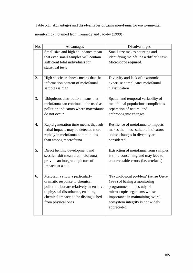
165

Table 5.1: Advantages and disadvantages of using meiofauna for environmental

monitoring (Obtained from Kennedy and Jacoby (1999)).

No. Advantages Disadvantages 1. Small size and high abundance mean

that even small samples will contain sufficient total individuals for statistical tests

Small size makes counting and identifying meiofauna a difficult task. Microscope required.

2. High species richness means that the information content of meiofaunal samples is high

Diversity and lack of taxonomic expertise complicates meiofaunal classification

3. Ubiquitous distribution means that meiofauna can continue to be used as pollution indicators where macrofauna do not occur

Spatial and temporal variability of meiofaunal populations complicates separation of natural and anthropogenic changes

4. Rapid generation time means that sub-lethal impacts may be detected more rapidly in meiofauna communities than among macrofauna

Resilience of meiofauna to impacts makes them less suitable indicators unless changes in diversity are considered

5. Direct benthic development and sessile habit mean that meiofauna provide an integrated picture of impacts at a site

Extraction of meiofauna from samples is time-consuming and may lead to uncorrectable errors (i.e. artefacts)

6. Meiofauna show a particularly dramatic response to chemical pollution, but are relatively insensitive to physical disturbance, enabling chemical impacts to be distinguished from physical ones

‘Psychological problem’ (sensu Giere, 1993) of basing a monitoring programme on the study of microscopic organisms whose importance in maintaining overall ecosystem integrity is not widely appreciated

166

5.5 Conclusions

There have been a number of previous studies of benthic marine pollution in

Antarctica to monitor and understand the ecological consequences of human

disturbance on the benthic community (Lenihan and Oliver, 1995, Lenihan, 1992,

Cripps and Shears, 1997, Duquesne and Riddle, 2002, Green and Nichols, 2004, Saul

et al., 2005). The human disturbances at Casey Station are caused mainly by routine

research station operations (such as sewage, small fuel and oil spills and emissions),

past waste disposal practices and shipping. Previous studies of shallow subtidal areas

near Casey Station have monitored the impacts on benthic ecosystems by studying

changes in benthic microbial, microalgae and macrofauna communities (Thompson et

al., 2006, Powell et al., 2005b, Stark et al., 2003c, Cunningham et al., 2005,

Cunningham et al., 2003, Stark et al., 2006, Stark et al., 2003b, Stark et al., 2003a,

Powell et al., 2005a, Thompson et al., 2007). By examining impacts on the

meiofaunal community, this thesis contributes to the understanding of the effects of

ongoing human impacts at Casey Station. It is apparent that there are effects on

benthic communities from station activities at all levels examined, from the

microscopic to the macroscopic.

The station activities at Casey have contributed to the contamination of the local

benthic ecosystem. Previous work on the benthic fauna in the marine environment

surrounding Casey station has shown differences in the infaunal communities that

were correlated with the presence of pollutants. The higher concentrations of

contamination are known to occur in sediments collected from bays adjacent to Casey

167

as compared to control locations located further afield (Stark et al., 2003b, Snape et

al., 2001, Cunningham et al., 2003). The contamination had caused change to the

benthic composition in many ways. Powell et al. (2003), in the microbial community,

heavy metals also appear to have some influence on the communities, particularly

iron, cadmium, manganese, zinc and arsenic. As for hydrocarbon contamination,

Powell (2005b) reported only minor changes occurred after 5 weeks in the microbial

communities in the sediment treated with Biodegradable, SAB, Clean and Used

lubricants. Their short-term experiment showed that SAB diesel appears to have

caused the biggest change in microbial component among other lubricant used. This

short-term changes were also observed in the diatom composition, whereby difference

in abundance between control and hydrocarbon contaminated treatment were visible

after 11 weeks exposure (Cunningham et al., 2003). Diatom community composition

also differed at disturbed locations in comparison to the control locations

(Cunningham et al., 2005). They noted that, in Brown Bay, metal concentration

particularly those of copper, iron, tin and lead are responsible for the large proportion

of variation in diatom community composition. Similarly, meiofaunal communities in

disturbed locations near Casey Station were different but had lower abundances than

at control locations. Similar findings have been found at other research stations

around the Antarctic continent, for example at McMurdo Station, the benthic

sediment is heavily contaminated with anthropogenic chemicals and the benthic

community is dominated by polychaete worms, which are opportunistic species

commonly found in polluted harbor habitats (Lenihan and Oliver, 1995, Lenihan,

1992). In general, the disturbed locations (sites near to Casey Station) had a lower

diversity of soft sediment macrofaunal assemblages, but often recorded higher

abundances of individuals (Stark et al., 2003b). It may be concluded that the presence

168

of contamination from the station activities causes the benthic community structure to

alter and reduces the biodiversity.

Different taxa responded differently to pollution and at least one group from each

community could be considered as an indicator taxa. Thus, presence or increase of

particular taxa may indicate contamination. For example taxa such as Orchomenella

franklini (gammarid) was very abundant in Brown Bay (impacted site) and was very

low or nearly absent in control sites (Stark et al., 2003c). This organism has low

abundance in O’Brien Bay which has less hydrocarbon and metal contamination by

comparison to Brown Bay where levels of hydrocarbons and metals are high.

Similarly in studies on diatom, Cunningham et al. (2005) found out that Navicula

were the indicator for the impacted sites. For example, N. directa and N. aff. glacei

showed a positive correlation with contamination in Brown Bay. Although diatoms

have been proven as an indicator for impacted sites, caution should be made in

making conclusion as species compositions were also affected by grain size and

effects of hydrocarbons also varies between types of hydrocarbon involved

(Cunningham et al., 2005). While, in this study on meiofauna, both genera from

nematodes Odonthophora and Paralinhomoes were considered as pollutant indicators.

Thus, monitoring the abundance of these taxa could be useful in future monitoring

programmes. By selecting particular groups or taxa to monitor, time consuming

laboratory work (identification of all organisms in community) could be avoided.

However, concentration of contaminants and other environmental variables should be

considered in all monitoring programmes.

169

Based on the monitoring studies at Casey station, it can be concluded that benthic

communities living in sediments are well-suited for environmental impact detection

and monitoring in Antarctica. They have a fixed spatial relationship with the source of

impact by comparison to those organisms which are mobile and/or live in the water

column. Whereby mobile organisms are able to avoid stressful condition by moving

out of the impacted area.

170

5.6 Future research

In this current study, the monitoring and evaluation of human impacts were based on

the meiofaunal community, providing useful information about the environmental

conditions at Casey Station. Furthermore by studying the meiofauna community at

Casey, a much broader context for environmental assessments has been obtained.

This study found some strong correlations between patterns of meiofaunal

assemblages and metal concentrations in sediments. However these are only

correlations and further work in the form of laboratory and/or field experiments are

needed to test the hypothesis that metals alter meiofaunal community structure and

composition. In particular meiofauna appear to be sensitive to Ag, As, Ba, Cd, Pb, Sn,

U, and Zn. Experiments using single metals or combinations of several metals would

be useful in testing whether it is metals and not some other environmental variable

influencing the observed patterns.

This study was not able to measure hydrocarbons in sediments and for future work it

would be useful to test whether there are also strong correlations between meiofaunal

assemblage patterns and the presence of hydrocarbons. Although hydrocarbons were

proven to affect communities in the field experiment, hydrocarbons are likely to co-

occur with metal pollution and it is uncertain which would have the greatest influence

on meiofaunal assemblages.

171

Meiofauna are a component of the benthic ecosystem that responds clearly to

anthropogenic disturbance as well as natural environmental fluctuations. Monitoring

meiofauna in environmental assessments would be a useful tool to include in such

studies in Antarctica.

To further study the effects of heavy metal and hydrocarbon pollutants on meiofauna,

it is recommended to use an individual taxa or species as well as experiments with

whole communities. Further questions that warrant investigation include:

1. At what concentration does metal contamination affect individual taxa and the

meiofaunal community?

2. How do different species respond to different levels of contamination?

3. Do meiofaunal communities recover from contamination and how long is the

recovery period?

4. Does the combination of multiple contaminants have synergistic effects that

are greater than single contaminants?

172

REFERENCES

Ahn, I. Y., Lee, S. H., Kim, K. T., Shim, J. H. & Kim, D. Y. (1996). Baseline heavy metal concentrations in the antarctic clam, Laternula elliptica in Maxwell Bay, King George Island, Antarctica. Marine Pollution Bulletin, 32, 592-598.

Aislabie, J. M., Balks, M. R., Foght, J. M. & Waterhouse, E. J. (2004). Hydrocarbon spills on Antarctic soils: effects and management. Environment Science and Technology 38, 1265-1274.

Alheit, J. & Scheibel, W. (1982). Benthic harpacticoids as a food source for fish. Marine Biology, 70, 141-147.

Allgen, C. (1930). Uber eine neue Art des Enoplolaimus de Man, E. gracilisetosus von Macquarie Inseln. Zoology Anz, 92, 89-190.

Alongi, D. M. & Pichon, M. (1988). Bathyal meiobenthos of the western Coral Sea: distribution and abundance in relation to microbial standing stocks and environmental factors. Deep Sea Research Part A. Oceanographic Research Papers, 35, 491-503.

Alongi, D. M. & Tietjen, J. H. (1990). Population Growth and Effects of Nematodes on Nutrient Regeneration and Bacteria Associated with Mangrove Detritus from Northeastern Queensland(Australia). Marine Ecology Progress Series MESEDT, 68.

Alves, A. S., Adão, H., Patrício, J., Neto, J. M., Costa, M. J. & Marques, J. C. (2009). Spatial distribution of subtidal meiobenthos along estuarine gradients in two southern European estuaries (Portugal). Journal of the Marine Biological Association of the UK, 1-12.

Anderson, M. J., Gorley, R. N. & Clarke, K. R. (2007). PERMANOVA+ for PRIMER: guide to software and statistical methods. PRIMER-E, Plymouth.

Armenteros, M., Martín, I., Williams, J. P., Creagh, B., González-Sansón, G. & Capetillo, N. (2006). Spatial and temporal variations of meiofaunal communities from the Western Sector of the Gulf of Batabanó, Cuba. I. Mangrove systems. Estuaries and Coasts, 29, 124-132.

Arnaud, P. M. (1974). Contribution It la bionomie marine benthique des regions Antarctiques et Subantarctiques. Tethys, 6, 456-656.

173

Austen, M. C. & Mcevoy, A. J. (1997). The use of offshore meiobenthic communities in laboratory microcosm experiments: response to heavy metal contamination. Journal of Experimental Marine Biology and Ecology, 211, 247-261.

Austen, M. C., Mcevoy, A. J. & Warwick, R. M. (1994). The specificity of meiobenthic community responses to different pollutants: results from microcosm experiments. Marine Pollution Bulletin, 28, 557-563.

Austen, M. C. & Widdicombe, S. (2006). Comparison of the response of meio-and macrobenthos to disturbance and organic enrichment. Journal of Experimental Marine Biology and Ecology, 330, 96-104.

Barnard, P. (1998). Biological diversity in Namibia: a clash of sea and land, fog and dust. Biodiversity and Conservation, 7, 415-417.

Beier, S. & Traunspurger, W. (2001). The meiofauna community of two small German streams as indicator of pollution. Journal of Aquatic Ecosystem Stress and Recovery (Formerly Journal of Aquatic Ecosystem Health), 8, 387-405.

Bejarano, A. C., Chandler, G. T., He, L. & Coull, B. C. (2006). Individual to population level effects of South Louisiana crude oil water accommodated hydrocarbon fraction (WAF) on a marine meiobenthic copepod. Journal of Experimental Marine Biology and Ecology, 332, 49-59.

Beyrem, H., Louati, H., Essid, N., Aïssa, P. & Mahmoudi, E. (2009). Effects of two lubricant oils on marine nematode assemblages in a laboratory microcosm experiment. Marine Environmental Research.

Beyrem, H., Mahmoudi, E., Essid, N., Hedfi, A., Boufahja, F. & Aissa, P. (2007). Individual and combined effects of cadmium and diesel on a nematode community in a laboratory microcosm experiment. Ecotoxicology and Environmental Safety, 68, 412-418.

Bick, A. & Arlt, G. (2005). Intertidal and subtidal soft-bottom macro-and meiofauna of the Kongsfjord (Spitsbergen). Polar Biology, 28, 550-557.

Boaden, P. J. S. (1980). Meiofaunal thiobios and “the Arenicola negation”: Case not proven. Marine Biology, 58, 25-29.

Bodin, P. (1988). Results of ecological monitoring of three beaches polluted by the Amoco Cadiz oil spill: Development of meiofauna from 1978 to 1984. Marine Ecology Progress Series. Oldendorf, 42, 105-123.

Bodin, P. (1997). Catalogue of the new marine harpacticoid copepods. Doc. Trav. Inst. Roy. Sci. Nat. Belg., 89, 304.

174

Borum, J. & Sand-Jensen, K. (1996). Is total primary production in shallow coastal marine waters stimulated by nitrogen loading? Oikos, 76, 406-410.

Bouvy, M. & Soyer, J. (1989). Benthic seasonality in an intertidal mud flat at Kerguelen Islands (Austral Ocean). The relationships between meiofaunal abundance and their potential microbial food. Polar Biology, 10, 19-27.

Bouwman, L. A., K. Romeyn, D. R. Kremer & F. B. Van Es (1984). Occurence and feeding biology of some nematode species in estuarine Aufwuchs communities. Cahiers de Biologie Marine XXV, 287-303.

Bradford, J. M. & Wells, J. B. J. (1983). New calanoid and harpacticoid copepods from beneath the Ross Ice Shelf, Antarctica. Polar Biology, 2, 1-15.

Brady, G. S. (1910). Die marinen Copepoden I. Deutche Sudpolar Expedition 1901-1903. Zooogy, 3, 497-594.

Brady, G. S. (1918). Australasian Antarctic Expedition 1911-1914.

Brandt, A., Andrew J. Gooday, Simone N. Branda˜O, Saskia Brix, Wiebke Bro¨Keland, Tomas Cedhagen, Madhumita Choudhury, Nils Cornelius, Bruno Danis, Ilse De Mesel, Robert J. Diaz, David C. Gillan, Brigitte Ebbe, John A. Howe, Dorte Janussen, Stefanie Kaiser, Katrin Linse, Marina Malyutina, Jan Pawlowski, Michael Raupach & Ann Vanreusel (2007). First insights into the biodiversity and biogeography of the Southern Ocean deep sea. Nature, 447, 307-311.

Bustos-Baez, S. & Frid, C. (2003). Using indicator species to assess the state of macrobenthic communities. Hydrobiologia, 496, 299-309.

Cabioch, L. (1980). Pollution of subtidal sediments and disturbance of benthic animal communities. Ambio, 294-296.

Calabretta, C. J. & Oviatt, C. A. (2008). The response of benthic macrofauna to anthropogenic stress in Narragansett Bay, Rhode Island: A review of human stressors and assessment of community conditions. Marine Pollution Bulletin, 56, 1680-1695.

Chinnadurai, G. & Fernando, O. J. (2007). Meiofauna of mangroves of the southeast coast of India with special reference to the free-living marine nematode assemblage. Estuarine, Coastal and Shelf Science, 72, 329-336.

Clarke, A. & Harris, C. M. (2003). Polar marine ecosystems: major threats and future change. Environmental Conservation, 30, 1-25.

175

Clarke, K. R. (1993). Non-parametric multivariate analyses of changes in community structure. Austral Ecology, 18, 117-143.

Clarke, K. R. & Ainsworth, M. (1993). A method of linking multivariate community structure to environmental variables. Marine Ecology Progress Series, 92, 205-205.

Clarke, K. R. & Gorley, R. N. (2006). PRIMER v6. User manual/tutorial. Plymouth routine in mulitvariate ecological research. Plymouth Marine Laboratory.

Clarke, K. R., Somerfield, P. J. & Gorley, R. N. (2008). Testing of null hypotheses in exploratory community analyses: similarity profiles and biota-environment linkage. Journal of Experimental Marine Biology and Ecology, 366, 56-69.

Clarke, K. R. & Warwick, R. M. (1994). Similarity-based testing for community pattern: the two-way layout with no replication. Marine Biology, 118, 167-176.

Clarke, K. R. & Warwick, R. M. (2001). Changes in marine communities: an approach to statistical analysis and interpretation.

Cobb, N. A. (1914). The North American free-living fresh-water nematodes. Transactions of the American Microscopical Society, 69-133.

Cobb, N. A. (1930). Marine free-living nematodes. Australasian Antarctic Expedition 1911-1914 6, 1-28.

Coull, B. C. (1988). 3. Ecology of the Marine Meiofauna. Introduction to the Study of Meiofauna. Washington, D.C, Smithsonian Institution Press.

Coull, B. C. (1990). Are members of the meiofauna food for higher trophic levels? Transactions of the American Microscopical Society, 109, 233-246.

Coull, B. C. & Bell, S. B. (1979). Perspectives of marine meiofaunal ecology. Marine Science, 10, 189-216.

Coull, B. C. & Chandler, G. T. (1992). Pollution and meiofauna: field, laboratory, and mesocosm studies. Oceanography and Marine Biology, 30, 191-271.

Coull, B. C., Hicks, G. R. F. & Wells, J. B. J. (1981). Nematode/copepod ratios for monitoring pollution: a rebuttal. Marine Pollution Bulletin, 12, 378-381.

Cripps, G. C. & Priddle, J. (1991). Review: Hydrocarbons in the Antarctic marine environment. Antarctic Science, 3, 233-250.

176

Cripps, G. C. & Shears, J. (1997). The fate in the marine environment of a minor diesel fuel spill from an Antarctic research station. Environmental monitoring and assessment, 46, 221-232.

Cunningham, L., Jonathan, S. S., Ian, S., Andrew, M. & Martin, J. R. (2003a). Effects of Metal and Petroleum Hydrocarbon Contamination on Benthic Diatom Communities Near Casey Station, Antarctica: An Experimental Approach. Journal of Phycology, 39, 490-503.

Cunningham, L. & Mcminn, A. (2004). The influence of natural enviromental factors on benthic diatom communities from the Windmill Islands, Antarctica. Phycologia, 43, 744-755.

Cunningham, L., Snape, I., Stark, J. S. & Riddle, M. J. (2005). Benthic diatom community response to environmental variables and metal concentrations in a contaminated bay adjacent to Casey Station, Antarctica. Marine Pollution Bulletin, 50, 264-275.

Cunningham, L., Stark, J. S., Snape, I., Mcminn, A. & Riddle, M. J. (2003b). Effects of metal and petroleum hydrocarbon contamination on benthic diatom communities near Casey Station, Antarctica: An experimental approach. Journal of Phycology, 39, 490-503.

Cunningham, L., Stark, J. S., Snape, I., Mcminn, A. & Riddle, M. J. (2003c). Effects of metal and petroleum hydrocarbon contamination on benthic diatom communities near Casey Station, Antarctica: an experimental approach. Journal of Phycology, 39, 490-503.

Da Rocha, C. M. C., Venekey, V., Bezerra, T. N. C. & Souza, J. R. B. (2006). Phytal marine nematode assemblages and their relation with the macrophytes structural complexity in a Brazilian tropical rocky beach. Hydrobiologia, 553, 219-230.

Dahms, H. U. (1989). First record of a lecithotrophic nauplius in Harpacticoida (Crustacea, Copepoda) collected from the Weddell Sea (Antarctica). Polar Biology, 10, 221-224.

Dahms, H. U., Bergmans, M. & Schminke, H. K. (1990). Distribution and adaptations of sea ice inhabiting Harpacticoida (Crustacea, Copepoda) of the Weddell Sea (Antarctica). Marine Ecology, 11, 207-226.

Dalto, A. G., Gremare, A., Dinet, A. & Fichet, D. (2006). Muddy-bottom meiofauna responses to metal concentrations and organic enrichment in New Caledonia South-West Lagoon. Estuarine Coastal and Shelf Science, 67, 629-644.

Danovaro, R., Croce, N. D., Eleftheriou, A., Fabiano, M., Papadopoulou, N., Smith, C. & Tselepides, A. (1995a). Meiofauna of the deep Eastern Mediterranean

177

Sea: distribution and abundance in relation to bacterial biomass, organic matter composition and other environmental factors. Progress in Oceanography, 36, 329-341.

Danovaro, R., Fabiano, M. & Vincx, M. (1995b). Meiofauna response to the Agip Abruzzo oil spill in subtidal sediments of the Ligurian Sea. Marine Pollution Bulletin, 30, 133-145.

De'ath, G. (2002). Multivariate regression trees: a new technique for modeling species-environment relationships. Ecology, 83, 1105-1117.

De Bovee, F. & Soyer, J. (1975). Le meiobenthos de l'Archipel de Kerguelen. Premieres donnees quantitatives. C. R. Hebd. Acad. Sc. Paris, 280, 2369-2372.

De Broyer, C., Bouquegneau, J. M., Dauby, P., De Ridder, C. & Vanreusel, A. (2007). Biodiversity of three representative groups of the Antarctic Zoobenthos: Comparative structure, distribution and function (BIANZO) EV/24. Belgian Science Policy.

De Leonardis, C., Sandulli, R., Vanaverbeke, J., Vicx, M. & De Zio, S. (2008). Meiofauna and nematode diversity in some Mediterranean subtidal areas of the Adriatic and Ionian Sea. Scientia Marina, 72.

De Ley, P. & Blaxter, M. (2004). A new system for Nematoda: combining morphological characters with molecular trees, and translating clades into ranks and taxa. Nematology Monographs and Perspectives, 2, 633–653.

De Mesel, I., Derycke, S., Swings, J., Vincx, M. & Moens, T. (2006a). Role of nematodes in decomposition processes: Does within-trophic group diversity matter? Marine Ecology Progress Series, 321, 157-166.

De Mesel, I., Lee, H. J., Vanhove, S., Vincx, M. & Vanreusel, A. (2006b). Species diversity and distribution within the deep-sea nematode genus Acantholaimus on the continental shelf and slope in Antarctica. Polar Biology, 29, 860-871.

De Skowronski, R. S. & Corbisier, T. N. (2002). Meiofauna distribution in Martel Inlet, King George Island (Antarctica): sediment features versus food availability. Polar Biology, 25, 126-134.

De Troch, M., Gurdebeke, S., Fiers, F. & Vincx, M. (2001). Zonation and structuring factors of meiofauna communities in a tropical seagrass bed (Gazi Bay, Kenya). Journal of Sea Research, 45, 45-61.

Delgado, J. D., Riera, R., Monterroso, Ó. & Núñez, J. (2009). Distribution and abundance of meiofauna in intertidal sand substrata around Iceland. Aquatic Ecology, 43, 221-233.

178

Deprez, P. P., Arens, M. & Locher, H. (1999). Identification and assessment of contaminated sites at Casey Station, Wilkes Land, Antarctica. Polar Record, 35, 299-316.

Deprez, T., Speybroeck, J., Steyaert, M. & Vincx, M. (2005). NeMys. World wide web electronic publication. www. nemys. ugent. be, version (1/2007).

Doulgeraki, S., Lampadariou, N. & Sinis, A. (2006). Meiofaunal community structure in three Mediterranean coastal lagoons (North Aegean Sea). Journal of the Marine Biological Association of the UK, 86, 209-220.

Drzyzga, O. (2003). Diphenylamine and derivatives in the environment: a review. Chemosphere, 53, 809-818.

Duquesne, S. & Liess, M. (2003). Increased sensitivity of the macroinvertebrate Paramorea walkeri to heavy-metal contamination in the presence of solar UV radiation in Antarctic shoreline waters. Marine Ecology Progress Series, 255, 183-191.

Duquesne, S. & Riddle, M. (2002). Biological monitoring of heavy-metal contamination in coastal waters off Casey Station, Windmill Islands, East Antarctica. Polar Biology, 25, 206-215.

Ellis, R. J., Neish, B., Trett, M. W., Best, J. G., Weightman, A. J., Morgan, P. & Fry, J. C. (2001). Comparison of microbial and meiofaunal community analyses for determining impact of heavy metal contamination. Journal of Microbiological Methods, 45, 171-185.

Essink, K. & Romeyn, K. (1994). Estuarine nematodes as indicators of organic pollution; an example from the Ems estuary (The Netherlands). Aquatic Ecology, 28, 213-219.

Fabiano, M. & Danovaro, R. (1999). Meiofauna distribution and mesoscale variability in two sites of the Ross Sea (Antarctica) with contrasting food supply. Polar Biology, 22, 115-123.

Fichet, D., Boucher, G., Radenac, G. & Miramand, P. (1999). Concentration and mobilisation of Cd, Cu, Pb and Zn by meiofauna populations living in harbour sediment: their role in the heavy metal flux from sediment to food web. Science of the Total Environment, The, 243, 263-272.

Field, J. G., Clarke, K. R. & Warwick, R. M. (1982). A practical strategy for analysing multispecies distribution patterns. Marine Ecology Progress Series, 8, 37-52.

Filler, D. M., Snape, I. & Barnes, D. L. (2008). Bioremediation of petroleum hydrocarbons in cold regions, Cambridge Univ Pr pp.

179

Fleeger, J. W. & Chandler, G. T. (1983). Meiofauna responses to an experimental oil spill in a Louisiana salt marsh. Marine Ecology Progress Series, 11, 257-264.

Fonseca, G., Vanreusel, A. & Decraemer, W. (2006). Taxonomy and biogeography of Molgolaimus Ditlevsen, 1921 (Nematoda : Chromadoria) with reference to the origins of deep sea nematodes. Antarctic Science, 18, 23-50.

Franco, M. (2007). Nematode response to changing food conditions in shallow marine and estuarine sediments. PhD Thesis, University of Gent.

Frithsen, J. B., Elmgren, R. & Rudnick, D. T. (1985). Responses of benthic meiofauna to long-term, low-level additions of no. 2 fuel oil. Marine Ecology Progress Series. Oldendorf, 23, 1-14.

Gallucci, F., Moens, T., Vanreusel, A. & Fonseca, G. (2008). Active colonisation of disturbed sediments by deep-sea nematodes: evidence for the patch mosaic model. Marine Ecology Progress Series, 367, 173-183.

Gambi, C., Vanreusel, A. & Danovaro, R. (2003). Biodiversity of nematode assemblages from deep-sea sediments of the Atacama Slope and Trench (South Pacific Ocean). Deep-Sea Research Part I-Oceanographic Research Papers, 50, 103-117.

Gambi, M. C., Lorenti, M., Russo, G. F. & Scipione, M. B. (2004). Benthic associations of the shallow hard bottoms off Terra Nova Bay, Ross Sea: Zonation, biomass and population structure. Antarctic Science, 6, 449-462.

Gee, J. M. (1989). An ecological and economic review of meiofauna as food for fish. Zoological Journal of the Linnean Society, 96, 243-261.

Gee, J. M. & Fleeger, J. W. (2008). Two new species of harpacticoid copepod from the South Orkney Islands, Antarctica, and a redescription of Idyellopsis typica Lang (Tisbidae). Biological Journal of the Linnean Society, 88, 143-165.

Gerdes, D., Hilbig, B. & Montiel, A. (2003). Impact of iceberg scouring on macrobenthic communities in the high-Antarctic Weddell Sea. Polar Biology, 26, 295-301.

Gerlach, S. A. (1971). On the importance of marine meiofauna for benthos communities. Oecologia, 6, 176-190.

Gerlach, S. A. & Schrage, M. (1971). Life cycles in marine meiobenthos. Experiments at various temperatures with Monhystera disjuncta and Theristus pertenuis (Nematoda). Marine Biology, 9, 274-280.

180

Gheskiere, T., Hoste, E., Vanaverbeke, J., Vincx, M. & Degraer, S. (2004). Horizontal zonation patterns and feeding structure of marine nematode assemblages on a macrotidal, ultra-dissipative sandy beach (De Panne, Belgium). Journal of Sea Research, 52, 211-226.

Gheskiere, T., Magda, V., Greet, P. & Steven, D. (2006). Are strandline meiofaunal assemblages affected by a once-only mechanical beach cleaning? Experimental findings. Marine Environmental Research, 61, 245-264.

Gheskiere, T., Vincx, M., Weslawski, J. M., Scapini, F. & Degraer, S. (2005). Meiofauna as descriptor of tourism-induced changes at sandy beaches. Marine environmental Research, 60, 245-265.

Giere, O. (1979). The impact of oil pollution on intertidal meiofauna. Field studies after the La Coruna spill, May, 1976. Cahiers de Biologie Marine Biodiversity, 20, 231-251.

Giere, O. (1993). Meiobenthology. The Microscopic Fauna in Aquatic Sediments. , Berlin : Springer-Verlag, 328 pp.

Giesbrecht, W. (1902). Resultas du voyage du S.Y.Belgica en1897-1899. Copepoden. Rapp. Sci.,Zool, 1-49.

Gobin, J. F. & Warwick, R. M. (2006). Geographical variation in species diversity: a comparison of marine polychaetes and nematodes. Journal of Experimental Marine Biology and Ecology, 330, 234-244.

Golemansky, V. & Chipev, N. (1999). Bulgarian Antarctic Research. Life Sciences. , Sofia, Pensoft Publishers, 114 pp.

Gomez Gesteira, J. L., Dauvin, J. C. & Salvande Fraga, M. (2003). Taxonomic level for assessing oil spill effects on soft-bottom sublittoral benthic communities. Marine Pollution Bulletin, 46, 562-572.

Gray, J. S. & Johnson, R. M. (1970). The bacteria of a sandy beach as an ecological factor affecting the interstitial gastrotrich Turbanella hyalina Schultze. Journal of Experimental Marine Biology and Ecology, 4, 119-133.

Green, G. & Nichols, P. D. (2004). Hydrocarbons and sterols in marine sediments and soils at Davis Station, Antarctica: a survey for human-derived contaminants. Antarctic Science, 7, 137-144.

Gregory, A. (2007). Response of macrobenthic communties to oil spills along Goa coast. MSc., Dissertation, National Institute of Oceanography, Mumbai University, Goa, India, 87pp.

181

Grove, S. L., Probert, P. K., Berkenbusch, K. & Nodder, S. D. (2006). Distribution of bathyal meiofauna in the region of the Subtropical Front, Chatham Rise, south-west Pacific. Journal of Experimental Marine Biology and Ecology, 330, 342-355.

Günther, S., George, K. H. & Gleitz, M. (1999). High sympagic metazoan abundance in platelet layers at Drescher Inlet, Weddell Sea, Antarctica. Polar Biology, 22, 82-89.

Gutt, J. & Piepenburg, D. (2003). Scale-dependent impact on diversity of Antarctic benthos caused by grounding of icebergs. Marine Ecology Progress Series, 253, 77-83.

Gutt, J., Starmans, A. & Dieckmann, G. (1996). Impact of iceberg scouring on polar benthic habitats. Marine Ecology Progress Series, 137, 311-316.

Gutzmann, E., Martínez Arbizu, P., Rose, A. & Veit-Köhler, G. (2004). Meiofauna communities along an abyssal depth gradient in the Drake Passage. Deep-Sea Research Part II, 51, 1617-1628.

Gyedu-Ababio, T. K. & Baird, D. (2006). Response of meiofauna and nematode communities to increased levels of contaminants in a laboratory microcosm experiment. Ecotoxicology and Environmental Safety, 63, 443-450.

Gyedu-Ababio, T. K., Furstenberg, J. P., Baird, D. & Vanreusel, A. (1999). Nematodes as indicators of pollution: a case study from the Swartkops River system, South Africa. Hydrobiologia, 397, 155-169.

Hack, L. A., Tremblay, L. A., Wratten, S. D., Lister, A. & Keesing, V. (2007). Benthic meiofauna community composition at polluted and non-polluted sites in New Zealand intertidal environments. Marine Pollution Bulletin, 54, 1801-1812.

Hedfi, A., Mahmoudi, E., Boufahja, F., Beyrem, H. & Aissa, P. (2007). Effects of Increasing Levels of Nickel Contamination on Structure of Offshore Nematode Communities in Experimental Microcosms. Bulletin of Environmental Contamination and Toxicology, 79, 345-349.

Heip, C., Huys, R., Vincx, M., Vanreusel, A., Smol, N., Herman, R. & Herman, P. M. J. (1990). Composition, distribution, biomass and production of North Sea meiofauna. Netherlands Journal of Sea Research, 26, 333-342.

Heip, C., Vincx, M. & Vranken, G. (1985). The ecology of marine nematodes. Oceanography and Marine Biology, 23, 399-489.

182

Heip, V. (1985). Vranken, 1985. C. Heip, M. Vincx and G. Vranken, The ecology of marine nematodes. Oceanography and Marine Biology Annual Review, 23, 399–489.

Heiri, O., Lotter, A. F. & Lemcke, G. (2001). Loss on ignition as a method for estimating organic and carbonate content in sediments: reproducibility and comparability of results. Journal of Paleolimnology, 25, 101-110.

Hendelberg, M. & Jensen, P. (1993). Vertical distribution of the nematode fauna in a coastal sediment influenced by seasonal hypoxia in the bottom water. Ophelia, 37, 83-94.

Herman, R. L. & Dahms, H. U. (1992). Meiofauna communities along a depth transect off Halley Bay (Weddell Sea-Antarctica). Polar Biology, 12, 313-320.

Hicks, G. R. F. (1988). Evolutionary implications of swimming behaviour in meiobenthic copepods. Hydrobiologia, 167, 497-504.

Higgins, R. P. & Thiel, H. (1988). Introduction to the study of meiofauna, Washington DC, Smithsonian Institution Press, 488 pp.

Hope, W. D. (1974). Deontostoma timmerchioi n. sp., a new marine nematode (Leptosomatidae) from Antarctica, with a note on the structure and possible function of the ventromedian supplement. . Trans. Amer. Micros. Soc. , 93 314-324.

Hoshiai, T., Tanimura, A. & Kudoh, S. (1996). The significance of autumnal sea ice biota in the ecosystem of ice-covered polar seas. National Institute of Polar Research Symposium Polar Biology, 9, 27-34.

Hoste, E., Vanhove, S., Schewe, I., Soltwedel, T. & Vanreusel, A. (2007). Spatial and temporal variations in deep-sea meiofauna assemblages in the Marginal Ice Zone of the Arctic Ocean. Deep Sea Research Part I: Oceanographic Research Papers, 54, 109-129.

Huys, R. & Conroy-Dalton, S. (2006). Comparative analysis of vermiform genera (Copepoda: Harpacticoida: Cylindropsyllidae), including descriptions of Boreovermis, new genus and Bolbotelos, new genus, from the Southern North Sea. Journal of Crustacean Biology, 26, 206-223.

Huys, R., Gee, J. M., Moore, C. G. & Hamond, R. (1996). Marine and brackish water harpacticoid copepods part 1: keys and notes for identification of the species, Synopses of the British fauna (New Series), 51. Field Studies Council: Shrewsbury, UK. 352 pp.

Inglis, W. G. (1958). A new species of the nematode genus Thoracostoma from the Antarctic. Antarctic. Ann. Mag. Nat. Hist. (13) 1, 45-48.

183

Ingole, B., Sivadas, S., Goltekar, R., Clemente, S., Nanajkar, M., Sawant, R., D'silva, C., Sarkar, A. & Ansari, Z. (2006). Ecotoxicological effect of grounded MV River Princess on the intertidal benthic organisms off Goa. Environment International, 32, 284-291.

James, R. J., Smith, M. P. L. & Fairweather, P. G. (1995). Sieve mesh-size and taxonomic resolution needed to describe natural spatial variation of marine macrofauna. Marine Ecology Progress Series, 118, 187-198.

Jansson, B. O. (1968). Quantitative and experimental studies of the interstitial fauna in four Swedish sandy beaches. Ophelia, 5, 1-71.

Kennedy, A. D. & Jacoby, C. A. (1999). Biological Indicators of Marine Environmental Health: Meiofauna–A Neglected Benthic Component? Environmental Monitoring and Assessment, 54, 47-68.

Kennish, M. J. (1998). Pollution impacts on marine biotic communities, New Jersey, CRC Press, 310 pp.

Kerry, E. (1993). Bioremediation of experimental petroleum spills on mineral soils in the Vestfold Hills, Antarctica. Polar Biology, 13, 163-170.

Kito, K., Shishida, Y. & Ohyama, Y. (1996). A new species of the genus Eudorylaimus Andrássy, 1959 (Nematoda: Qudsianematidae) from East Antarctica. Polar Biology, 16, 163-169.

Kotwicki, L., Szymelfenig, M., De Troch, M. & Zajaczkowski, M. (2004). Distribution of meiofauna in Kongsfjorden, Spitsbergen. Polar Biology, 27, 661-669.

Lakhan, V. C., Cabana, K. & Lavalle, P. D. (2003). Relationship between grain size and heavy metals in sediments from beaches along the coast of Guyana. Journal of Coastal Research, 600-608.

Lambshead, P. J. D. (1984). The nematode/copepod ratio: some anomalous results from the Firth of Clyde. Marine Pollution Bulletin, 15, 256-259.

Lang, K. (1934). Marine Harpacticiden von der Campbell-Inseln und einigen anderen sudlichen Inseln., Lunds Univ. Arsskr. N.F.Avd.

Lang, K. (1936). Copepoda Harpacticoidea. Further zoological results of the Swedish Antarctic Expedition 1901-1903. IN S. (Ed.). Stockholm, P.A Norstedt & Sponer.

184

Larner, B. L., Seen, A. J. & Snape, I. (2006). Evaluation of diffusive gradients in thin film (DGT) samplers for measuring contaminants in the Antarctic marine environment. Chemosphere, 65, 811-820.

Leduc, D. & Probert, P. K. (2009). The effect of bacterivorous nematodes on detritus incorporation by macrofaunal detritivores: A study using stable isotope and fatty acid analyses. Journal of Experimental Marine Biology and Ecology, 371, 130-139.

Lee, H., Vanhove, S., Peck, L. S. & Vincx, M. (2001a). Recolonisation of meiofauna after catastrophic iceberg scouring in shallow Antarctic sediments. Polar Biology, 24, 918-925.

Lee, H. J., Gerdes, D., Vanhove, S. & Vincx, M. (2001b). Meiofauna response to iceberg disturbance on the Antarctic continental shelf at Kapp Norvegia (Weddell Sea). Polar Biology, 24, 926-933.

Lee, H. J. & Van De Velde, J. (1999). Biodiversity of Antarctic nematodes. IN W.E., A. & J., G. (Eds.) Reports on polar research, the Expedition ANTARKTIS ZX/3 (EASIZ II). Bremerhaven, Boehl & Oppermann,.

Lee, M. R., Correa, J. A. & Castilla, J. C. (2001c). An assessment of the potential use of the nematode to copepod ratio in the monitoring of metals pollution. The Chanaral case. Marine Pollution Bulletin, 42, 696-701.

Lee, R. F. & Page, D. S. (1997). Petroleum hydrocarbons and their effects in subtidal regions after major oil spills. Marine Pollution Bulletin, 34, 928-940.

Lenihan, H. S. (1992). Benthic marine pollution around McMurdo Station, Antarctica: a summary of findings. Marine Pollution Bulletin, 25, 318-323.

Lenihan, H. S. & Oliver, J. S. (1995). Anthropogenic and natural disturbances to marine benthic communities in Antarctica. Ecological Applications, 311-326.

Levinton, J. S. (1995). Marine biology: function, biodiversity, ecology, Oxford University Press 420 pp.

Linstow, O. V. (1907). Nematodes of the Scottish National Antarctic Expedition 1902-1904. Edinburgh, Proceedings of the Royal Society.

Lorenzen, S., Prein, M. & Valentin, C. (1987). Mass aggregations of the free-living marine nematode Pontonema vulgare (Oncholaimidae) in organically polluted fjords. Marine Ecology Progress Series, 37, 27-34.

Mahmoudi, E., Essid, N., Beyrem, H., Hedfi, A., Boufahja, F., Vitiello, P. & Aissa, P. (2005). Effects of hydrocarbon contamination on a free living marine

185

nematode community: Results from microcosm experiments. Marine Pollution Bulletin, 50, 1197-1204.

Mahmoudi, E., Essid, N., Beyrem, H., Hedfi, A., Boufahja, F., Vitiello, P. & Aissa, P. (2007). Individual and combined effects of lead and zinc on a free-living marine nematode community: Results from microcosm experiments. Journal of Experimental Marine Biology and Ecology, 343, 217-226.

Mamilov, A. S. & Dilly, O. M. (2002). Soil microbial eco-physiology as affected by short-term variations in environmental conditions. Soil Biology and Biochemistry, 34, 1283-1290.

Mani, E. P., Ravikumar, B., Antony, P. J., Lyla, P. S. & Khan, S. A. (2008). Impact of physical disturbance on the community structure of estuarine Benthic Meiofauna. Asian Journal of Scientific Research, 1, 239-245.

Mawson, P. M. (1958a). Free-living nematodes section 2: Additional Enoploidea from Antarctic stations. Rep. B.A.N.Z. Antarct. Res. Exped., 6, 291-305.

Mawson, P. M. (1958b). Free-living nematodes section 3: Additional Enoploidea from Antarctic stations. Rep. B.A.N.Z. Antarct. Res. Exped., 6, 307-358.

Mclachlan, A. (1978). A quantitative analysis of the meiofauna and the chemistry of the redox potential discontinuity zone in a sheltered sandy beach. Estuarine and Coastal Marine Science, 7, 275-290.

Mclachlan, A., Winter, P. E. D. & Botha, L. (1977). Vertical and horizontal distribution of sub-littoral meiofauna in Algoa Bay, South Africa. Marine Biology, 40, 355-364.

Mcminn, A., Gibson, J., Hodgson, D. & Aschman, J. (1995). Nutrient limitation in Ellis Fjord, eastern Antarctica. Polar Biology, 15, 269-276.

Mcminn, A. & Hodgson, D. (1993). Summer phytoplankton succession in Ellis Fjord, eastern Antarctica. Journal of Plankton Research, 15, 925.

Mcminn, A., Runcie, J. W. & Riddle, M. (2004). Effect of seasonal sea ice breakout on the photosynthesis of benthic diatom mats at Casey, Antarctica. Journal of Phycology, 40, 62-69.

Millward, R. N., Carman, K. R., Fleeger, J. W., Gambrell, R. P. & Portier, R. (2004). Mixtures of metals and hydrocarbons elicit complex responses by a benthic invertebrate community. Journal of Experimental Marine Biology and Ecology, 310, 115-130.

186

Millward, R. N., Carman, K. R., Fleeger, J. W., Gambrell, R. P., Powell, R. T. & Rouse, M. A. M. (2001). Linking ecological impact to metal concentrations and speciation: a microcosm experiment using a salt marsh meiofaunal community. Environmental Toxicology and Chemistry, 20, 2029-2037.

Millward, R. N. & Grant, A. (2000). Pollution-induced tolerance to copper of nematode communities in the severely contaminated Restronguet creek and adjacent estuaries, Cornwall, United Kingdom. Environmental Toxicology and Chemistry, 19, 454-461.

Mirto, S., La Rosa, T., Gambi, C., Danovaro, R. & Mazzola, A. (2002). Nematode community response to fish-farm impact in the western Mediterranean. Environmental Pollution, 116, 203-214.

Moens, T., Verbeeck, L., De Mayer, A., Swings, J. & Vincx, M. (1999). Selective attraction of marine bacterivorous nematodes to their bacterial food. Marine Ecology Progress Series.

Moens, T. & Vincx, M. (2009). Observations on the feeding ecology of estuarine nematodes. Journal of the Marine Biological Association of the UK, 77, 211-227.

Monard, T. & Dollfus, R. (1932). Sur quelques animaux rapportes par E. Aubert de la Rue des Iles australes (Kerguelen et St Paul). Bull.Soc.Zool. France, 57, 21-28.

Moore, C. G. & Bett, B. J. (1989). The use of meiofauna in marine pollution impact assessment. Zoological Journal of the Linnean Society, 96, 263-280.

Moreno, M., Albertelli, G. & Fabiano, M. (2009). Nematode response to metal, PAHs and organic enrichment in tourist marinas of the mediterranean sea. Marine Pollution Bulletin, 58, 1192-1201.

Moreno, M., Ferrero, T. J., Gallizia, I., Vezzulli, L., Albertelli, G. & Fabiano, M. (2008a). An assessment of the spatial heterogeneity of environmental disturbance within an enclosed harbour through the analysis of meiofauna and nematode assemblages. Estuarine, Coastal and Shelf Science, 77, 565-576.

Moreno, M., Vezzulli, L., Marin, V., Laconi, P., Albertelli, G. & Fabiano, M. (2008b). The use of meiofauna diversity as an indicator of pollution in harbours. ICES Journal of Marine Science, 65, 1428.

Ndaro, S. G. M. & Ólafsson, E. (1999). Soft-bottom fauna with emphasis on nematode assemblage structure in a tropical intertidal lagoon in Zanzibar, eastern Africa: I. Spatial variability. Hydrobiologia, 405, 133-148.

187

Nicholas, W. L. & Hodda, M. (1999). The free-living nematodes of a temperate, high energy, sandy beach: faunal composition and variation over space and time. Hydrobiologia, 394, 113-127.

Pearson, T. H. & Rosenberg, R. (1978). Macrobenthic succession in relation to organic enrichment and pollution of the marine environment. Oceanography and Marine Biology,16, 229-311.

Peck, L. S., Brockington, S., Vanhove, S. & Beghyn, M. (1999). Community recovery following catastrophic iceberg impacts in a soft-sediment shallow-water site at Signy Island, Antarctica. Marine Ecology-Progress Series, 186, 1-8.

Peterson, C. H., Kennicutt Jr, M. C., Green, R. H., Montagna, P., Harper Jr, D. E., Powell, E. N. & Roscigno, P. F. (1996). Ecological consequences of environmental perturbations associated with offshore hydrocarbon production: A perspective on long-term exposures in the Gulf of Mexico. Canadian Journal of Fisheries and Aquatic Sciences, 53, 2637-2654.

Pfannkuche, O. & Thiel, H. (1987). Meiobenthic stocks and benthic activity on the NE-Svalbard Shelf and in the Nansen Basin. Polar Biology, 7, 253-266.

Pfannkuche, O., Thiel, H. & Samples, M. (1988). 9. Sample processing Introduction to the Study of Meiofauna. Washington DC, Smithsonian Institution Press.

Pihl, L. & Rosenberg, R. (1984). Food selection and consumption of the shrimp Crangon crangon in some shallow marine areas in western Sweden. Marine ecology progress series. Oldendorf, 15, 159-168.

Platonova, T. A. (1958). Contribution to the Nematode fauna of the family Leptosomatidae from Kerguelen Island (in Russian). Inf. Byull. Sov. Antarkt. Eksped. 1955-1958, 3, 59-61.

Platt, H. M., Shaw, K. M. & Lambshead, P. J. D. (1984). Nematode species abundance patterns and their use in the detection of environmental perturbations. Hydrobiologia, 118, 59-66.

Platt, H. M. & Warwick, R. M. (1983). Free-living marine nematodes. Part I. British enoploids. Cambridge University Press, Cambridge.

Powell, S. A., Snape, I., Bowman, J. P., Thompson, B. A. W., Stark, J. S., Mccammon, S. A. & Riddle, M. J. (2005a). A comparison of the short term effects of diesel fuel and lubricant oils on Antarctic benthic microbial communities. Journal of Experimental Marine Biology and Ecology, 322, 53-65.

188

Powell, S. M., Bowman, J. P., Snape, I. & Stark, J. S. (2003). Microbial community variation in pristine and polluted nearshore Antarctic sediments. FEMS Microbiology Ecology, 45, 135-145.

Powell, S. M., Harvey, P. M., Stark, J. S., Snape, I. & Riddle, M. J. (2007). Biodegradation of petroleum products in experimental plots in Antarctic marine sediments is location dependent. Marine Pollution Bulletin, 54, 434-440.

Powell, S. M., Snape, I., Bowman, J. P., Thompson, B. A. W., Stark, J. S., Mccammon, S. A. & Riddle, M. J. (2005b). A comparison of the short term effects of diesel fuel and lubricant oils on Antarctic benthic microbial communities. Journal of Experimental Marine Biology and Ecology, 322, 53-65.

Pusceddu, A., Gambi, C., Zeppilli, D., Bianchelli, S. & Danovaro, R. (2009). Organic matter composition, metazoan meiofauna and nematode biodiversity in Mediterranean deep-sea sediments. Deep Sea Research Part II: Topical Studies in Oceanography, 56, 755-762.

Quidor, M. (1920). Copepodes- Expedition Antarctique Francaise 1903-1905, 56 pp.

Raes, M., Rose, A. & Vanreusel, A. (2010). Response of nematode communities after large-scale ice-shelf collapse events in the Antarctic Larsen area. Global Change Biology, 16, 1618-1631.

Raffaelli, D. G. & Mason, C. F. (1981). Pollution monitoring with meiofauna, using the ratio of nematodes to copepods. Marine Pollution Bulletin, 12, 158-163.

Raghukumar, C., Bharathi, P. A. L., Ansari, Z. A., Nair, S., Ingole, B., Sheelu, G., Mohandass, C., Nagender Nath, B. & Rodrigues, N. (2001). Bacterial standing stock, meiofauna and sediment–nutrient characteristics: indicators of benthic disturbance in the Central Indian Basin. Deep-Sea Research Part II, 48, 3381-3399.

Reimnitz, E., Barnes, P. W., Toimil, L. J. & Melchior, J. (1977). Ice gouge recurrence and rates of sediment reworking, Beaufort Sea, Alaska. Geology, 5, 405.

Reise, K. & Ax, P. (1979). A meiofaunal “thiobios” limited to the anaerobic sulfide system of marine sand does not exist. Marine Biology, 54, 225-237.

Rodri´Guez, J. G., Lastra, M. & López, J. (2003). Meiofauna distribution along a gradient of sandy beaches in northern Spain. Estuarine, Coastal and Shelf Science, 58, 63-69.

Rudnick, D. T., Elmgren, R. & Frithsen, J. B. (1985). Meiofaunal prominence and benthic seasonality in a coastal marine ecosystem. Oecologia, 67, 157-168.

189

Saul, D. J., Aislabie, J. M., Brown, C. E., Harris, L. & Foght, J. M. (2005). Hydrocarbon contamination changes the bacterial diversity of soil from around Scott Base, Antarctica. FEMS Microbiology Ecology, 53, 141-155.

Saunders, J. E., Al Zahed, K. M. & Paterson, D. M. (2007). The impact of organic pollution on the macrobenthic fauna of Dubai Creek (UAE). Marine Pollution Bulletin, 54, 1715-1723.

Schiemer, F., Novak, R. & Ott, J. (1990). Metabolic studies on thiobiotic free-living nematodes and their symbiotic microorganisms. Marine Biology, 106, 129-137.

Schnack-Schiel, S. B., Dieckmann, G. S., Gradinger, R., Melnikov, I., Spindler, M. & Thomas, D. N. (2001a). Meiofauna in sea ice of the Weddell Sea (Antarctica). Polar Biology, 24, 724-728.

Schnack-Schiel, S. B., Dieckmann, G. S., Gradinger, R., Melnikov, I. A., Spindler, M. & Thomas, D. N. (2001b). Meiofauna in sea ice of the Weddell Sea (Antarctica). Polar Biology, 24, 724-728.

Schnack-Schiel, S. B., Haas, C., Michels, J., Mizdalski, E., Schünemann, H., Steffens, M. & Thomas, D. N. (2008). Copepods in sea ice of the western Weddell Sea during austral spring 2004. Deep-Sea Research Part II, 55, 1056-1067.

Schratzberger, M., Dinmore, T. & Jennings, S. (2002). Impacts of trawling on the diversity, biomass and structure of meiofauna assemblages. Marine Biology, 140, 83-93.

Schratzberger, M., Gee, J. M., Rees, H. L., Boyd, S. E. & Wall, C. M. (2001). The structure and taxonomic composition of sublittoral meiofauna assemblages as an indicator of the status of marine environments. Journal of the Marine Biological Association of the UK, 80, 969-980.

Schratzberger, M. & Jennings, S. (2002). Impacts of chronic trawling disturbance on meiofaunal communities. Marine Biology, 141, 991-1000.

Schratzberger, M., Warr, K. & Rogers, S. I. (2006). Patterns of nematode populations in the southwestern North Sea and their link to other components of the benthic fauna. Journal of Sea Research, 55, 113-127.

Schunemann, H., Steffens, M. & Thomas, D. N. (2008). Copepods in sea ice of the western Weddell Sea during austral spring 2004. Deep-Sea Research, 2, 1056-1067.

Schuurmans-Stekhoven, J. H. & Mawson, P. M. (1955). On some free-living Nematodes from Kerguelen Island. T. Helminth, 29, 87-104.

190

Sebastian, S., Raes, M., De Mesel, I. & Vanreusel, A. (2007). Comparison of the nematode fauna from the Weddell Sea abyssal plain with two North Atlantic abyssal sites. Deep-Sea Research Part II-Topical Studies in Oceanography, 54, 1727-1736.

Seifried, S. (2004). The importance of a phylogenetic system for the study of deep-sea harpacticoid diversity. Zoological Studies, 43, 435-445.

Sellanes, J. & Neira, C. (2006). ENSO as a natural experiment to understand environmental control of meiofaunal community structure. Marine Ecology, 27, 31-43.

Ser, M. E. F. (1991). Meiofauna of an experimental soft bottom ecosystem-effects of macrofauna and cadmium exposure. Marine Ecology Progress Series, 70, 245-255.

Shiells, G. M. & Anderson, K. J. (1985). Pollution Monitoring Using the Nematode/Copepod Ratio, A Practical Application. Marine Pollution Bulletin, 16.

Shirayama, Y. (1984). The abundance of deep sea meiobenthos in the western Pacific in relation to environmental factors. Oceanologica acta, 7, 113-121.

Shirayama, Y. & Kojima, S. (1994). Abundance of deep-sea meiobenthos off Sanriku, Northeastern Japan. Journal of Oceanography, 50, 109-117.

Simboura, N. & Zenetos, A. (2002). Benthic indicators to use in ecological quality classification of Mediterranean soft bottom marine ecosystems, including a new biotic index. Mediterranean Marine Science, 3, 77-112.

Snape, I., Riddle, M. J., Stark, J. S., Cole, C. M., King, C. K., Duquesne, S. & Gore, D. B. (2001). Management and remediation of contaminated sites at Casey Station, Antarctica. Polar Record, 37, 199-214.

Snape, I., Scouller, R. C., Stark, S. C., Stark, J., Riddle, M. J. & Gore, D. B. (2004). Characterisation of the dilute HCl extraction method for the identification of metal contamination in Antarctic marine sediments. Chemosphere, 57, 491-504.

Snedecor, G. W. & Cochran, W. G. (1980). Statistical methods The Iowa State University Press. , 507p.

Soetaert, K. & Heip, C. (1995). Nematode assemblages of deep-sea and shelf break sites in the North Atlantic and Mediterranean Sea. Marine Ecology Progress Series. Oldendorf, 125, 171-183.

191

Soetaert, K., Vincx, M., Wittoeck, J. & Tulkens, M. (1995). Meiobenthic distribution and nematode community structure in five European estuaries. Hydrobiologia, 311, 185-206.

Somerfield, P. J., Gee, J. M. & Warwick, R. M. (1994). Soft sediment meiofaunal community structure in relation to a long-term heavy metal gradient in the Fal estuary system. Marine Ecology Progress Series. Oldendorf, 105, 79-88.

Soyer, J. (1985). Mediterranean Sea meiobenthos. In: Mediterranean Marine Ecosystems (eds M. Moraitou- Apostolopoulou & V. Kiortsis) , Plenum, New York, 85–108

Stark, J. S. (1998). Heavy metal pollution and macrobenthic assemblages in soft

sediments in two Sydney estuaries, Australia. Marine and Freshwater Research, 49, 533-540.

Stark, J. S. (2000). The distribution and abundance of soft-sediment macrobenthos around Casey Station, East Antarctica. Polar Biology, 23, 840-850.

Stark, J. S., Riddle, M. J. & Simpson, R. D. (2003a). Human impacts in soft-sediment assemblages at Casey Station, East Antarctica: Spatial variation, taxonomic resolution and data transformation. Austral Ecology, 28, 287-304.

Stark, J. S., Riddle, M. J. & Smith, S. D. A. (2004). Influence of an Antarctic waste dump on recruitment to nearshore marine soft-sediment assemblages. Marine Ecology Progress Series, 276, 53-70.

Stark, J. S., Riddle, M. J., Snape, I. & Scouller, R. C. (2003b). Human impacts in Antartic marine soft-sediment assemblages: Correlations between multivariate biological patterns and environmental variables at Casey Station. Estuarine, Coastal and Shelf Science, 56, 717-734.

Stark, J. S., Snape, I. & Riddle, M. J. (2003c). The effects of petroleum hydrocarbon and heavy metal contamination of marine sediments on recruitment of Antarctic soft-sediment assemblages: A field experimental investigation. Journal of Experimental Marine Biology and Ecology, 283, 21-50.

Stark, J. S., Snape, I. & Riddle, M. J. (2006). Abandoned Antarctic waste disposal sites: Monitoring remediation outcomes and limitations at Casey Station. Ecological Management and Restoration, 7, 21-31.

Stark, J. S., Snape, I., Riddle, M. J. & Stark, S. C. (2005). Constraints on spatial variability in soft-sediment communities affected by contamination from an Antarctic waste disposal site. Marine Pollution Bulletin, 50, 276-290.

Steiner, G. (1931a). Die Nematoden der Deutschen Sudpolar-Expedition 1901-1903. I. Teil. Dt. Sudpol.-Exped., 20, 167-216.

192

Steiner, G. (1931b). Die Nematoden der Deutschen Sudpolar-Expedition 1901-1903. II. Teil. Dt. Sudpol.-Exped., 20, 305-433.

Steyaert, M., Deprez, T., Raes, M., Bezerra, T., Demesel, I., Derycke, S., Desmet, G., Fonseca, G., Franco, M. A. & Gheskiere, T. (2005). Electronic key to the free-living marine. Nematodes. http://nemys.ugent.be/.

Steyaert, M., Garner, N., Van Gansbeke, D. & Vincx, M. (1999). Nematode communities from the North Sea: environmental controls on species diversity and vertical distribution within the sediment. Journal of the Marine Biological Association of the UK, 79, 253-264.

Steyaert, M., Vanaverbeke, J., Vanreusel, A., Barranguet, C., Lucas, C. & Vincx, M. (2003). The importance of fine-scale, vertical profiles in characterising nematode community structure. Estuarine Coastal and Shelf Science, 58, 353-366.

Suchanek, T. H. (1994). Temperate coastal marine communities: biodiversity and threats. Integrative and Comparative Biology, 34, 100.

Sutherland, T. F., Levings, C. D., Petersen, S. A., Poon, P. & Piercey, B. (2007). The use of meiofauna as an indicator of benthic organic enrichment associated with salmonid aquaculture. Marine Pollution Bulletin, 54, 1249-1261.

Swadling, K. (2001). Population structure of two Antarctic ice-associated copepods, Drescheriella glacialis and Paralabidocera antarctica, in winter sea ice. Marine Biology, 139, 597-603.

Swadling, K. M., Mcphee, A. D. & Mcminn, A. (2000). Spatial distribution of copepods in fast ice of eastern Antarctica. Polar Bioscience, 55-65.

Tam, N. F. Y. & Wong, Y. S. (2000). Spatial variation of heavy metals in surface sediments of Hong Kong mangrove swamps. Environmental Pollution, 110, 195-205.

Tenore, K. R., Tietjen, J. H. & Lee, J. J. (1977). Effect of meiofauna on incorporation of aged eelgrass, Zostera marina, detritus by the polychaete Nephthys incisa. Journal of the Fisheries Research Board of Canada, 34, 563-567.

Thompson, B. A. W., Davies, N. W., Goldsworthy, P. M., Riddle, M. J., Snape, I. & Stark, J. S. (2006). In situ lubricant degradation in antarctic marine sediments. 1. Short-term changes. Environmental Toxicology and Chemistry, 25, 356-366.

Thompson, B. A. W., Goldsworthy, P. M., Riddle, M. J., Snape, I. & Stark, J. S. (2007). Contamination effects by a ‘conventional’and a ‘biodegradable’lubricant oil on infaunal recruitment to Antarctic sediments: A

193

field experiment. Journal of Experimental Marine Biology and Ecology, 340, 213-226.

Thompson, B. W., Riddle, M. J. & Stark, J. S. (2003). Cost-efficient methods for marine pollution monitoring at Casey Station, East Antarctica: The choice of sieve mesh-size and taxonomic resolution. Marine Pollution Bulletin, 46, 232-243.

Tietjen, J. H. (1980). Population structure and species composition of the free-living nematodes inhabiting sands of the New York Bight Apex. Estuarine and Coastal Marine Science, 10, 61-73.

Timm, R. W. (1970). A revision of the nematode order Desmoscolecida Filipjev, 1929. University of California Publications in Zoology., 93, 1-115.

Timm, R. W. & Viglierohio, D. R. (1970). Studies of Antarctic nematodes. Antarctic Journal. U.S., 5, 135.

Tin, T., Fleming, Z. L., Hughes, K. A., Ainley, D. G., Convey, P., Moreno, C. A., Pfeiffer, S., Scott, J. & Snape, I. (2008). Impacts of local human activities on the Antarctic environment. Antarctic Science, 21, 3-33.

Townsend, A. T. (1999). The determination of arsenic and selenium in standard reference materials using sector field ICP-MS in high resolution mode. Fresenius' Journal of Analytical Chemistry, 364, 521-526.

Townsend, A. T. (2000). The accurate determination of the first row transition metals in water, urine, plant, tissue and rock samples by sector field ICP-MS. Journal of Analytical Atomic Spectrometry, 15, 307-314.

Underwood, A. J. (1981). Techniques of analysis of variance in experimental marine biology and ecology. Oceanography and Marine Biology: An Annual Review, 19, 513-605

Underwood, A. J. & Chapman, M. G. (1998). GMAV5 for Windows., Institute of Marine Ecology, University of Sydney, Australia.

Urban-Malinga, B., Wiktor, J., Jablonska, A. & Moens, T. (2005). Intertidal meiofauna of a high-latitude glacial Arctic fjord (Kongsfjorden, Svalbard) with emphasis on the structure of free-living nematode communities. Polar Biology, 28, 940-950.

Van Gaever, S., Vanreusel, A., Hughes, J. A., Bett, B. J. & Kiriakoulakis, K. (2004). The macro-and micro-scale patchiness of meiobenthos associated with the Darwin Mounds (north-east Atlantic). Journal of the Marine Biological Association of the UK, 84, 547-556.

194

Van Holsbeke, K. (1988). Analysis of community attributes of the benthic meiofauna of Frierfjordllangesundf jord. Marine Ecology Progress Series, 46, 171-180.

Vanaverbeke, J., Arbizu, P. M., Dahms, H. U. & Schminke, H. K. (1997a). The metazoan meiobenthos along a depth gradient in the Arctic Laptev Sea with special attention to nematode communities. Polar Biology, 18, 391-401.

Vanaverbeke, J., Soetaert, K., Heip, C. & Vanreusel, A. (1997b). The metazoan meiobenthos along the continental slope of the Goban Spur (NE Atlantic). Journal of Sea Research, 38, 93-107.

Vanhove, S., Arntz, W. & Vincx, M. (1999). Comparative study of the nematode communities on the southeastern Weddell Sea shelf and slope (Antarctica). Marine Ecology Progress Series, 181, 237-256.

Vanhove, S., Beghyn, M., Van Gansbeke, D., Bullough, L. W. & Vincx, M. (2000). A seasonally varying biotope at Signy Island, Antarctic: implications for meiofaunal structure. Marine Ecology Progress Series, 202, 13-25.

Vanhove, S., Lee, H. J., Beghyn, M., Van Gansbeke, D., Brockington, S. & Vincx, M. (1998). The metazoan meiofauna in its biogeochemical environment: The case of an Antarctic coastal sediment. Journal of the Marine Biological Association of the United Kingdom, 78, 411-434.

Vanhove, S., Vermeeren, H. & Vanreusel, A. (2004). Meiofauna towards the South Sandwich Trench (750–6300m), focus on nematodes. Deep-Sea Research Part II, 51, 1665-1687.

Vanhove, S., Wittoeck, J., Desmet, G., Van Den Berghe, B., Herman, R. L., Bak, R. P. M., Nieuwland, G., Vosjan, J. H., Boldrin, A. & Rabitti, S. (1995). Deep-sea meiofauna communities in Antarctica: structural analysis and relation with the environment. Marine Ecology Progress Series, 127, 65-76.

Vanreusel, A. (1990). Ecology of the free-living marine nematodes from the Voordelta (Southern Bight of the North Sea). I. Species composition and structure of the nematode communities. Cahiers de Biologie Marine, 31, 439-462.

Vanreusel, A. (1991). Ecology of free-living marine nematodes in the Voordelta (Southern bight of the north sea). II, Habitat preferences of the dominant species. Nematologica (Leiden), 37, 343-359.

Vanreusel, A., Andersen, A. C., Boetius, A., Connelly, D., Cunha, M. R., Decker, C., Hilario, A., Kormas, K. A., Maignien, L. S., Olu, K., Pachiadaki, M., Ritt, B., Rodrigues, C., Sarrazin, J., Tyler, P., Van Gaever, S. & Vanneste, H. (2009). Biodiversity of cold seep ecosystems along the European Margins. Oceanography, 22, 110-127.

195

Vanreusel, A., Clough, L., Jacobsen, K., Ambrose, W., Jivaluk, J., Ryheul, V., Herman, R. & Vincx, M. (2000). Meiobenthos of the central Arctic Ocean with special emphasis on the nematode community structure. Deep-Sea Research Part I: Oceanographic Research Papers, 47, 1855-1879.

Vanreusel, A., Vandenbossche, I. & Thiermann, F. (1997). Free-living marine nematodes from hydrothermal sediments: similarities with communities from diverse reduced habitats. Marine Ecology Progress Series, 157, 207-219.

Vanreusel, A., Vincx, M., Schram, D. & Vangansbeke, D. (1995). On the Vertical-Distribution of the Metazoan Meiofauna in Shelf Break and Upper Slope Habitats of the NE Atlantic. Internationale Revue Der Gesamten Hydrobiologie, 80, 313-326.

Veiga, P., Rubal, M. & Besteiro, C. (2009). Shallow sublittoral meiofauna communities and sediment polycyclic aromatic hydrocarbons (PAHs) content on the Galician coast (NW Spain), six months after the Prestige oil spill. Marine Pollution Bulletin, 58, 581-588.

Veit-Kohler, G. (2005). Influence of biotic and abiotic sediment factors on abundance and biomass of harpacticoid copepods in a shallow Antarctic bay. Scientia Marina, 69, 135-145.

Veit-Kohler, G. & Fuentes, V. (2007). A new pelagic Alteutha (Copepoda : Harpacticoida) from Potter Cove, King George Island, Antarctica - description, ecology and information on its year round distribution. Hydrobiologia, 583, 141-163.

Veit-Köhler, G., Laudien, J., Knott, J., Velez, J. & Sahade, R. (2008). Meiobenthic colonisation of soft sediments in arctic glacial Kongsfjorden (Svalbard). Journal of Experimental Marine Biology and Ecology, 363, 58-65.

Vermeeren, H., Vanreusel, A. & Vanhove, S. (2004). Species distribution within the free-living marine nematode genus Dichromadora in the Weddell Sea and adjacent areas. Deep-Sea Research Part II-Topical Studies in Oceanography, 51, 1643-1664.

Vezzulli, L., Fabiano, M., Granelli, V. & Moreno, M. (2003). Influence of large-spectrum environmental contamination on the micro–meiobenthic assemblages in harbour sediments of the ligurian sea (W Mediterranean). Chemistry and Ecology, 19, 233-246.

Vincx, M., Bett, B. J., Dinet, A., Ferrero, T., Gooday, A. J., Lambshead, P. J. D., Pfannkuche, O., Soltwedel, T. & Vanreusel, A. (1994). Meiobenthos of the Deep Northeast Atlantic. Advances in Marine Biology, 30, 1-88.

196

Vincx, M., Bett, B.J., Dinet, A., Ferrero, T., Gooday, A.J.,, Lambshead, P. J. D., Pfannkuche, O., Soltwedel, T., Vanreusel, & A. (1994.). Meiobenthos of the deep northeast Atlantic. Advances in Marine Biology, 30, 1-88.

Vincx, M. & Heip, C. (1991). The use of meiobenthos in pollution monitoring studies: a review. ICES Journal of Marine Science. 16, 50-67.

Voudrias, E. A. & Smith, C. L. (1986). Hydrocarbon pollution from marinas in estuarine sediments. Estuarine Coastal and Shelf Science ECSSD 3, 22.

Warwick, R. M. (1981). The influence of temperature and salinity on energy partitioning in the marine nematode Diplolaimelloides bruciei. Oecologia, 51, 318-325.

Warwick, R. M. (1986a). A new method for detecting pollution effects on marine macrobenthic communities. Marine Biology, 92, 557-562.

Warwick, R. M. (1986b). A new method for detecting pollution effects on marine macrobenthic communities. Marine Biology, 92, 557-562.

Warwick, R. M. (1988). The level of taxonomic discrimination required to detect pollution effects on marine benthic communities. Marine Pollution Bulletin, 19, 259-268.

Warwick, R. M. & Clarke, K. R. (1995). New'biodiversity' measures reveal a decrease in taxonomic distinctness with increasing stress. Marine Ecology Progress Series, 129, 301-305.

Warwick, R. M. & Clarke, K. R. (1998). Taxonomic distinctness and environmental assessment. Journal of Applied Ecology, 532-543.

Warwick, R. M., Joint, I. R. & Radford, P. J. (1979). Ecological processes in coastal environments. IN Jefferies, R. L. & Davey, A. J. (Eds.). Oxford, Blackwell.

Wells, J. B. J. (1978). Keys to aid in the identification of marine harpacticoid copepods amendment Bulletin Number 1-5. Zoology, 1-11.

Werner, I. & Martinez Arbizu, P. (1999). The sub-ice fauna of the Laptev Sea and the adjacent Arctic Ocean in summer 1995. Polar Biology, 21, 71-79.

Wieser, W., Ott, J., Schiemer, F. & Gnaiger, E. (1974). An ecophysiological study of some meiofauna species inhabiting a sandy beach at Bermuda. Marine Biology, 26, 235-248.

197

Witthoft-Muhlmann, A., Traunspurger, W. & Rothhaupt, K. O. (2005). Meiobenthic response to river-borne benthic particulate matter-a microcosm experiment. Freshwater Biology, 50, 1548-1559.

Wormald, A. P. (1976). Effect of an oil spill of marine diesel oil on meiofauna of a sandy beach at Picnic Bay, Hong Kong. Environmental Pollution, 11, 117-130.

Yin, X., Liu, X., Sun, L., Zhu, R., Xie, Z. & Wang, Y. (2006). A 1500-year record of lead, copper, arsenic, cadmium, zinc level in Antarctic seal hairs and sediments. The Science of the Total Environment , 371, 252-257.

meliofaunal communities and human impacts at casey station ... · meiofaunal communities and human...

Documents