Medical StatisticsMedical StatisticsMedical StatisticsMedical StatisticsProf.Amany Rashad Aboel-Seoud Prof.Amany Rashad Aboel-Seoud

Community Medicine DepartmentCommunity Medicine Department

Zagazig University,EGYPTZagazig University,EGYPT

Objectives:Objectives:•Define statistics, describe its uses in Define statistics, describe its uses in community medicinecommunity medicine•Summarize data in tables and graphsSummarize data in tables and graphs•Calculate measures of central tendency Calculate measures of central tendency and measures of dispersion.and measures of dispersion.•Describe normal distribution curve and its Describe normal distribution curve and its usesuses

Definition of statisticsDefinition of statistics

• It is the science and art of dealing It is the science and art of dealing with numbers.with numbers.

• Used for collection, summarization, Used for collection, summarization, presentation and analysis of data to presentation and analysis of data to get information based on objective get information based on objective basis (un-biased).basis (un-biased).

Uses of statistics

• Descriptive information for any population

• Prioritization of problems

• Prove association between variables

• Prove relation between risk and disease

• Compare new rates with old ones

• Compare local results with foreign ones

• Evaluate health programs & services

Medical Statistics

STATISTICAL ANALYSIS

usefulINFORMATIONIn medical field

DATA(accuracy)

DATA

SOURCESRecords, Census

Survey, Research studies(sampling)

PRESENTATIONTables

SummarizationGraphs

Analysis & interpretation

information

Planning for health programs

Types of dataTypes of data

Any collected observation will be eitherAny collected observation will be either Quantitative (numbers) either:Quantitative (numbers) either:1)Discrete (no fraction): as number of 1)Discrete (no fraction): as number of patients, hospital beds, RBCspatients, hospital beds, RBCs2)Continuous (with fraction): as hormone level, 2)Continuous (with fraction): as hormone level,

temperature, blood pressure, age temperature, blood pressure, age Qualitative (names or order)Qualitative (names or order) * categorical : black/white, male/female, yes/no* categorical : black/white, male/female, yes/no * ordinal : grade of tumor, SE standard * ordinal : grade of tumor, SE standard

Presentation of data

In tables In graphs They must have title, self explanatory clear, fully labeled, not complicated. Summarization of data by few

numbers as average, percentile, variance.

Table (1):Percentage distribution of the studied group in relation to sex

Observation (variable) (parameter) Sex

Number examined(No.)

Frequency (%)

MaleFemale

2030

4060

Total 50 100

Table ( ): Percentage distribution of the studied Table ( ): Percentage distribution of the studied group in relation to sex and agegroup in relation to sex and age

Age/yearAge/year malesmales femalesfemales

No.No. %% No.No. %%

<10<10

10 –10 –

20 –20 –

30 –30 –

40 –40 –

50 +50 +

Total Total

88

22

55

1212

1313

1010

5050

1616

44

1010

2424

2626

2020

100100

66

55

44

33

44

33

2525

2424

2020

1616

1212

1616

1212

100100

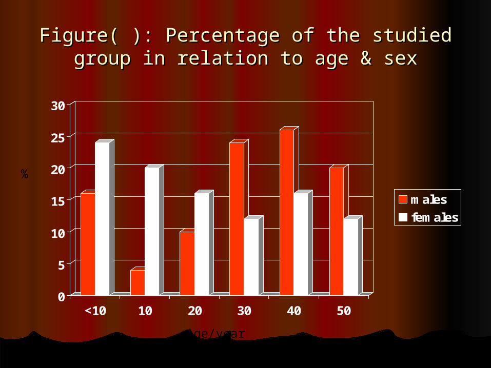
Figure( ): Percentage of the studied group in Figure( ): Percentage of the studied group in relation to age & sexrelation to age & sex

0

5

10

15

20

25

30

<10 10 20 30 40 50

males

females

%

Age/year

40%

22%

8%

10%

20%

gastroentr. chest inf.congenital anomal. accidentsothers

Fig.( ):Body temperature of 3 patients 4hours after polio vaccination

33

34

35

36

37

38

39

40

41

42

1 2 3 4

mohamed

ahmed

mostafa

hours

Temp.

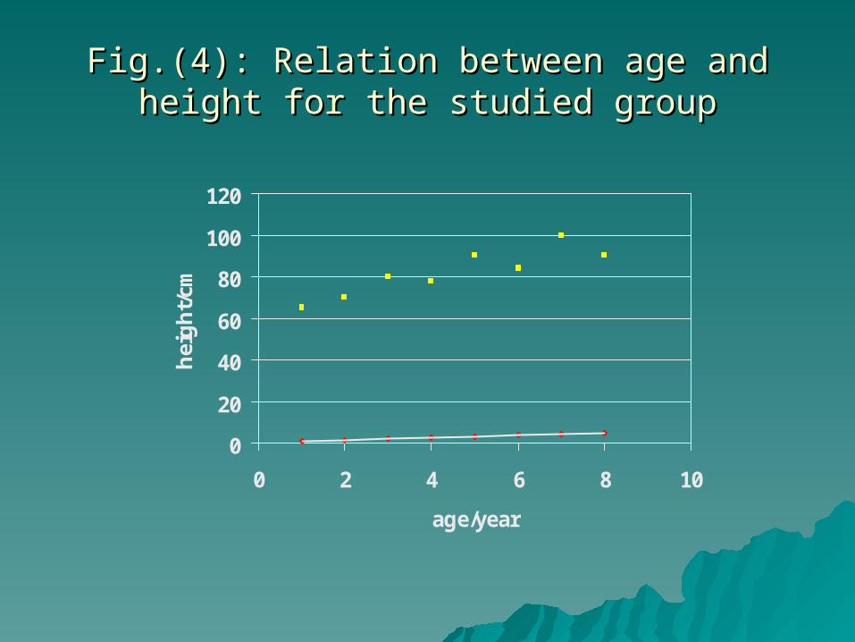
Fig.(4): Relation between age and height for the Fig.(4): Relation between age and height for the studied groupstudied group

0

20

40

60

80

100

120

0 2 4 6 8 10

age/year

hei

gh

t/cm

Fig.(8): frequency distribution of cases in relation to Fig.(8): frequency distribution of cases in relation to weightweight

0102030405060708090

freq

uen

cy o

f ca

ses

30 40 50 60

weight/kg

Fig.(5): Comparison between countries in relation Fig.(5): Comparison between countries in relation to socio-economic standardsto socio-economic standards

0%

10%

20%

30%

40%

50%

60%

70%

80%

90%

100%

%

England Germany Egypt Pakistan

low high

Data summarizationData summarization• PercentilePercentile

• QuartileQuartile

• Measures of central tendencyMeasures of central tendency

** mean **median **mode** mean **median **mode

• Measures of dispersionMeasures of dispersion

**range **variance **SD**range **variance **SD

** SE **co-efficient of ** SE **co-efficient of variationvariation

PercentilePercentile

• In In Ordered dataOrdered data

• 4- 6- 7- 8- 9- 10- 12- 13- 14- 20- 22 4- 6- 7- 8- 9- 10- 12- 13- 14- 20- 22

• 0-10-20-30-40-50- 60- 70- 80- 90-1000-10-20-30-40-50- 60- 70- 80- 90-100

• 10 is the 5010 is the 50thth percentile of these data percentile of these data

• 6 is the 106 is the 10thth percentile percentile

• 9 is the 409 is the 40thth percentile percentile

• We usually use the 25We usually use the 25thth, 50, 50thth and the 75 and the 75thth percentiles for data summarization=quartile.percentiles for data summarization=quartile.

1-1-The arithmetic mean:The arithmetic mean:

• Which is the sum of observation divided by the Which is the sum of observation divided by the number of observations:number of observations:

• x = ∑ x x = ∑ x • nn• Where : x = meanWhere : x = mean• ∑ ∑ denotes the (sum of)denotes the (sum of)• x the values of observation x the values of observation • n the number of observationn the number of observation• Example: In a study the age of 5 students were: 12 , 15, Example: In a study the age of 5 students were: 12 , 15,

10, 17, 1310, 17, 13• Mean = sum of observations / number of observationsMean = sum of observations / number of observations• Then the mean X = (12 + 15 + 10 + 17 + 13) / 5 =13.4 Then the mean X = (12 + 15 + 10 + 17 + 13) / 5 =13.4

yearsyears

2- Median:2- Median:It is the middle observation in a series of observation after It is the middle observation in a series of observation after

arranging them in an ascending or descending manner.arranging them in an ascending or descending manner.• The rank of median is (n + 1)/2 if the number of The rank of median is (n + 1)/2 if the number of

observation is odd and n/2 if the number is even (n = number of observation is odd and n/2 if the number is even (n = number of observation).observation).

If number of observation is odd, the median will be calculated as follow:If number of observation is odd, the median will be calculated as follow:Calculate the median of the following data 5, 6, 8, 9, 11 n = 5Calculate the median of the following data 5, 6, 8, 9, 11 n = 5The rank of the median = n + 1 / 2 i.e. (5+ 1)/ 2 = 3 . The median is the third The rank of the median = n + 1 / 2 i.e. (5+ 1)/ 2 = 3 . The median is the third

value in these groups when data are arranged in ascending (or value in these groups when data are arranged in ascending (or descending) manner.descending) manner.

So the median is 8 (the third value)So the median is 8 (the third value)• If the number of observation is even, the median will be calculated as If the number of observation is even, the median will be calculated as

follows:follows: e.g. 5, 6, 8, 9 e.g. 5, 6, 8, 9 n = 4 n = 4 • - The rank of median = n / 2 i.e. 4 / 2 = 2 .The median is the second - The rank of median = n / 2 i.e. 4 / 2 = 2 .The median is the second

value of that group. If data are arranged ascendingly then the median value of that group. If data are arranged ascendingly then the median will be 6 and if arranged descendingly the median will be 8 therefore will be 6 and if arranged descendingly the median will be 8 therefore the median will be the mean of both observations i.e. (6 + 8)/2 =7. For the median will be the mean of both observations i.e. (6 + 8)/2 =7. For simplicity we can apply the same equation used for odd numbers i.e. n simplicity we can apply the same equation used for odd numbers i.e. n + 1 / 2. The median rank will be 4 + 1 /2 = 2 ½ i.e. the median will be + 1 / 2. The median rank will be 4 + 1 /2 = 2 ½ i.e. the median will be the second and the third values i.e. 6 and 8, take their mean = 7. the second and the third values i.e. 6 and 8, take their mean = 7.

3- Mode3- Mode

• The most frequent occurring value in the The most frequent occurring value in the data is the mode and is calculated as data is the mode and is calculated as follows: follows:

• Example: 5, 6, 7, 5, 10. The mode in this Example: 5, 6, 7, 5, 10. The mode in this data is 5 since number 5 is repeated twice. data is 5 since number 5 is repeated twice. Sometimes, there is more than one mode Sometimes, there is more than one mode and sometimes there is no mode especially and sometimes there is no mode especially in small set of observations. Example : 20 , in small set of observations. Example : 20 , 18 , 14, 20, 13, 14, 30, 19. There are two 18 , 14, 20, 13, 14, 30, 19. There are two modes 14 and 20.modes 14 and 20.

• Example : 300, 280 , 130, 125 , 240 , 270 . Example : 300, 280 , 130, 125 , 240 , 270 . Has no mode.Has no mode.

2- Measures of 2- Measures of dispersiondispersion

• The measure of dispersion describes The measure of dispersion describes the degree of variations or scatter or dispersion of the degree of variations or scatter or dispersion of the data around its central values(dispersion = the data around its central values(dispersion = variation = spread = scatter).variation = spread = scatter).

• Range:Range:• It is the difference between the largest and It is the difference between the largest and

smallest values. It is the simplest measure of smallest values. It is the simplest measure of variation. Its disadvantages is that, it is based variation. Its disadvantages is that, it is based only on two of the observations and gives no idea only on two of the observations and gives no idea of how the other observations are arranged of how the other observations are arranged between these two. Also, it tends to be large between these two. Also, it tends to be large when the size of the sample increases.when the size of the sample increases.

Variance:Variance:• If we want to get the average of If we want to get the average of

differences between the mean and each differences between the mean and each observation in the data, we have to deduce each observation in the data, we have to deduce each value from the mean value from the mean and then sum these differences and divide it by and then sum these differences and divide it by the number of observation.the number of observation.

• i.e. Variance V = ∑ (mean – x) / ni.e. Variance V = ∑ (mean – x) / nThe value of this equation will be equal to zero The value of this equation will be equal to zero because the differences between each value and because the differences between each value and the mean will have negative and positive signs the mean will have negative and positive signs that will equalize zero on algebraic summation. that will equalize zero on algebraic summation.

• Therefore to overcome this zero we square the Therefore to overcome this zero we square the difference between the mean and each value so difference between the mean and each value so the sign will be always positive. Thus we get:the sign will be always positive. Thus we get:

• V = ∑ (mean – x)2 / n - 1V = ∑ (mean – x)2 / n - 1

3- Standard deviation3- Standard deviation• ::• The main disadvantage of the The main disadvantage of the

variance is that it is the square of the variance is that it is the square of the units used. So, it is more convenient to units used. So, it is more convenient to express the variation in the original express the variation in the original units by taking the square root of the units by taking the square root of the variance. This is called the standard variance. This is called the standard deviation (SD). Therefore SD = √ V deviation (SD). Therefore SD = √ V

• i.e. SD = i.e. SD = √ ∑ (mean – x)2 / n - 1√ ∑ (mean – x)2 / n - 1

4- Coefficient of 4- Coefficient of variation:variation:• The coefficient of variation expresses the standard The coefficient of variation expresses the standard

deviation as a percentage of the sample mean.deviation as a percentage of the sample mean.• C. V = SD / mean C. V = SD / mean ** 100 100 • C.V is useful when, we are interested in the relative size of C.V is useful when, we are interested in the relative size of

the variability in the data. the variability in the data. • Example : if we have observations 5, 7, 10, 12 and 16. Their Example : if we have observations 5, 7, 10, 12 and 16. Their

mean will be 50/5=10. SD = √ (25+9 +0 + 4 + 36 ) / (5-1) mean will be 50/5=10. SD = √ (25+9 +0 + 4 + 36 ) / (5-1) = √ 74 / 4 = 4.3= √ 74 / 4 = 4.3

• C.V. = 4.3 / 10 x 100 = 43%C.V. = 4.3 / 10 x 100 = 43%• Another observations are 2, 2, 5, 10, and 11. Their mean = Another observations are 2, 2, 5, 10, and 11. Their mean =

30 / 5 = 630 / 5 = 6• SD = √ (16 + 16 + 1 + 16 + 25)/(5 –1) = √ 74 / 4 = 4.3 SD = √ (16 + 16 + 1 + 16 + 25)/(5 –1) = √ 74 / 4 = 4.3 • C.V = 4.3 /6 x 100 = 71.6 %C.V = 4.3 /6 x 100 = 71.6 %• Both observations have the same SD but they are different Both observations have the same SD but they are different

in C.V. because data in the first group is homogenous (so in C.V. because data in the first group is homogenous (so C.V. is not high), while data in the second observations is C.V. is not high), while data in the second observations is heterogenous (so C.V. is high).heterogenous (so C.V. is high).

ExampleExample

• Summarize the following hemoglobin readings: Summarize the following hemoglobin readings: 9,8,10,9,7,11,12.9,8,10,9,7,11,12.

• Mean=9+8+10+9+7+11+12=66/7=9.4Mean=9+8+10+9+7+11+12=66/7=9.4• Median=n+1/2 = 7+1 /2=4Median=n+1/2 = 7+1 /2=4thth • 7,8,9,9,10,11,12 median=97,8,9,9,10,11,12 median=9• Mode=9Mode=9• Range=12 – 7=5Range=12 – 7=5• Variance=(9.4-9)2 +(9.4-8)2 +(9.4-10)2 ...Variance=(9.4-9)2 +(9.4-8)2 +(9.4-10)2 ...• /7-1=2.92/7-1=2.92• SD=square root of variance(2.92)=1.71SD=square root of variance(2.92)=1.71• SE = SD/sq.root of 7=1.71/2.64=0.64SE = SD/sq.root of 7=1.71/2.64=0.64• CV = SD / 9.4 x 100 =1.71/9.4=18.2%CV = SD / 9.4 x 100 =1.71/9.4=18.2%

Normal distribution curve

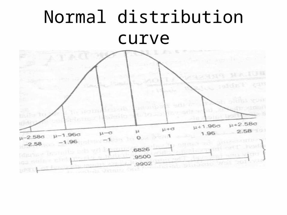
Normal distribution curveNormal distribution curve

• Mean, median and mode coincideMean, median and mode coincide

• Bell shape, symmetrical Bell shape, symmetrical

• Never endsNever ends

• 68% of population lies between mean + 68% of population lies between mean + SDSD

• 95% of population lies between mean 95% of population lies between mean +2SD+2SD

• 99% lies between mean+3SD99% lies between mean+3SD