medicaid as an investment in children: … · medicaid as an investment in children: what is the...
TRANSCRIPT
NBER WORKING PAPER SERIES
MEDICAID AS AN INVESTMENT IN CHILDREN:WHAT IS THE LONG-TERM IMPACT ON TAX RECEIPTS?
David W. BrownAmanda E. Kowalski
Ithai Z. Lurie
Working Paper 20835http://www.nber.org/papers/w20835
NATIONAL BUREAU OF ECONOMIC RESEARCH1050 Massachusetts Avenue
Cambridge, MA 02138January 2015
We thank participants at UCLA Anderson, the University of Connecticut, the University of Kentucky,Vanderbilt, and Yale for helpful comments. Kate Archibald, William Bishop, Anna Cornelius-Schecter,Rebecca McKibbin, and Sam Moy provided excellent research assistance. National Science Foundation(NSF) CAREER Award 1350132 and the National Institute on Aging of the National Institutes ofHealth (NIH) Award P30AG12810 supported Amanda Kowalski's work on this project. The findings,interpretations, and conclusions expressed in this paper are entirely those of the authors and do notnecessarily represent the views of the US Department of Treasury, the NSF, the NIH, or the NationalBureau of Economic Research.
NBER working papers are circulated for discussion and comment purposes. They have not been peer-reviewed or been subject to the review by the NBER Board of Directors that accompanies officialNBER publications.
© 2015 by David W. Brown, Amanda E. Kowalski, and Ithai Z. Lurie. All rights reserved. Short sectionsof text, not to exceed two paragraphs, may be quoted without explicit permission provided that fullcredit, including © notice, is given to the source.
Medicaid as an Investment in Children: What is the Long-Term Impact on Tax Receipts?David W. Brown, Amanda E. Kowalski, and Ithai Z. LurieNBER Working Paper No. 20835January 2015JEL No. H2,I1,I38
ABSTRACT
We examine the long-term impact of expansions to Medicaid and the State Children's Health InsuranceProgram that occurred in the 1980's and 1990's. With administrative data from the IRS, we calculatelongitudinal health insurance eligibility from birth to age 18 for children in cohorts affected by theseexpansions, and we observe their longitudinal outcomes as adults. Using a simulated instrument thatrelies on variation in eligibility by cohort and state, we find that children whose eligibility increasedpaid more in cumulative taxes by age 28. These children collected less in EITC payments, and thewomen had higher cumulative wages by age 28. Incorporating additional data from the Medicaid StatisticalInformation System (MSIS), we find that the government spent $872 in 2011 dollars for each additionalyear of Medicaid eligibility induced by the expansions. Putting this together with the estimated increasein tax payments discounted at a 3% rate, assuming that tax impacts are persistent in percentage terms,the government will recoup 56 cents of each dollar spent on childhood Medicaid by the time thesechildren reach age 60. This return on investment does not take into account other benefits that accruedirectly to the children, including estimated decreases in mortality and increases in college attendance.Moreover, using the MSIS data, we find that each additional year of Medicaid eligibility from birthto age 18 results in approximately 0.58 additional years of Medicaid receipt. Therefore, if we scaleour results by the ratio of beneficiaries to eligibles, then all of our results are almost twice as large.
David W. BrownDepartment of the Treasury1500 Pennsylvania Avenue, NWRoom 1217AWashington, D.C. [email protected]
Amanda E. KowalskiDepartment of EconomicsYale University37 Hillhouse AvenueBox 208264New Haven, CT 06520and [email protected]
Ithai Z. LurieDepartment of the Treasury1500 Pennsylvania Avenue NWWashington, DC [email protected]
1 Introduction
With the ongoing implementation of the Affordable Care Act (ACA) of 2010, the United
States is poised to experience a large increase in health insurance coverage. The literature
provides some evidence on the short term impacts of increases in health insurance coverage,
but it is possible that some of the most important gains from health insurance coverage
manifest themselves in the long term, after prolonged exposure. Although we will not know
the realized long term impacts of the ACA for many years to come, we can examine the long
term impact of previous health insurance expansions now.
Using data from the Internal Revenue Service (IRS), we examine the long term impact
of expansions to Medicaid that occurred in the 1980’s and 1990’s. Medicaid, a public health
insurance program for low income persons, began almost 50 years ago in 1965. It expanded
dramatically in the 1980’s and again in the 1990’s with the establishment of the State Chil-
dren’s Health Insurance Program (SCHIP) in 1997. These combined “Medicaid” expansions
resulted in a tremendous amount of variation in health insurance eligibility for similar chil-
dren in different states and birth cohorts. Some children affected by these expansions have
reached age 31 in our data, allowing us to examine outcomes for them as adults. Our main
outcomes of interest include net tax receipts, Earned Income Tax Credit (EITC) receipts,
wages, mortality, and college attendance.
One reason why we might expect to observe long term impacts of Medicaid expansions
is that a very large literature demonstrates robust short-term impacts of health insurance
expansions on coverage and on a small variety of other outcomes. Seminal papers by Janet
Currie and Jonathan Gruber examine a doubling of childhood eligibility between 1984 and
1992 (Currie and Gruber, 1996b) and the inclusion of pregnant women in coverage beginning
in 1985 (Currie and Gruber, 1996a). Pioneering the use of a simulated instrument methodol-
ogy that isolates policy variation, they find that Medicaid eligibility increased utilization of
medical care and reduced childhood and infant mortality. Card and Shore-Sheppard (2004)
focus on children’s eligibility increases induced by two federal expansions included in the
Currie and Gruber (1996b) analysis and find that the eligibility increases had modest im-
pacts on contemporaneous health insurance coverage, but they do not examine any other
outcomes. Several other papers revisit these expansions and later SCHIP expansions, all
finding impacts on coverage, generally from 5 to 24 percent.1
Beyond coverage, a small number of papers have found contemporaneous impacts on other
outcomes that could be potential mechanisms for long term health impacts. For example,
1See Blumberg et al. (2000); Rosenbach et al. (2001); Zuckerman and Lutzky (2001); Cunningham et al.(2002a); Cunningham et al. (2002b); Lo Sasso and Buchmueller (2004); Ham and Shore-Sheppard (2005);Hudson et al. (2005); Bansak and Raphael (2006); Buchmueller et al. (2008); and Gruber and Simon (2008).
2
Lurie (2009) finds evidence of increased doctor visits as a result of Medicaid expansions,
and Joyce and Racine (2003) find evidence of higher vaccination rates in response to the
same expansions. Beyond direct impacts on health care utilization, Yelowitz (1998) finds
that parents whose children who are exposed to Medicaid expansions are more likely to be
married, and Gruber and Yelowitz (1999) find that parents with access to public health
insurance save more, potentially making college more accessible to their children.
Bolstering the previous quasi-experimental literature, findings from recent Oregon Health
Insurance Experiment of 2008, in which the state of Oregon expanded coverage to childless
adults through a lottery, demonstrate short-term impacts of Medicaid expansions on a large
variety of outcomes, also suggesting that long-term impacts could be possible in our setting.2
However, the long term impact of the Oregon Health Insurance Experiment will not be known
until more time has passed. Moreover, two years after the health insurance eligibility lottery
took place, individuals who were randomized out of the lottery became eligible, so future
estimates of the long term impact of the Oregon Health Insurance Experiment will only
reflect up to two years of additional coverage for the lottery winners.
One advantage of the expansions that we study is that they resulted in several years of
expanded eligibility for the same children. Therefore, our results can potentially shed light
on the policy-relevant impact of expanding health insurance eligibility for all of childhood, as
opposed to the impact of expanding health insurance eligibility for a single year of childhood.
Given that our intervention occurred over a longer time period than other interventions
examined in the literature, we are also potentially more likely to observe long-term impacts.
Although most existing literature examines the impact of Medicaid expansions contem-
poraneously or within two years of the expansion, we are aware of a small number of papers
that examine the impact of health insurance expansions several years after the expansions
occurred. These papers provide other potential mechanisms for our findings. Meyer and
Wherry (2012) revisit one of the federal expansions examined by Card and Shore-Sheppard
(2004) with Vital Statistics data, which allows them to examine childhood and teen mortal-
ity after the expansions. They find a decrease in mortality for black teens, but they cannot
reject increases for white teens. Sommers et al. (2012), examine the impact of much more
recent expansions in Medicaid eligibility in three states since the year 2000, and they find
reductions in mortality up to five years after the expansion. Levine and Schanzenbach (2009)
examine the impact of availability of SCHIP and Medicaid at birth on children’s test scores
2Results from the first year after the experiment provide evidence that increased Medicaid eligibility ledto increased health insurance coverage, increased medical utilization, increased emergency room visits, lowerout-of-pocket medical expenditures, and better self-reported health (Finkelstein et al. (2012) and Taubmanet al. (2014)). Results from two years after the experiment show decreases in depression, increased use ofpreventive services, and no impact on clinical measures of cholesterol and diabetes (Baicker et al., 2013b).There are no detectable impacts on labor market participation or earnings (Baicker et al., 2013a).
3
and find an impact on reading scores but not math scores. Recent work by Cohodes et al.
(2014) finds that childhood exposure to Medicaid increases schooling, and other recent work
by Miller and Wherry (2014) finds that in utero exposure to Medicaid decreases obesity
and some types of hospitalizations in adulthood. However, impacts of Medicaid on adult
economic outcomes are hard to find. Boudreaux (2014) examines the impact of the stag-
gered adoption of Medicaid by states on later life economic outcomes for children exposed
to Medicaid during childhood but does not find any statistically significant impacts, likely
because the Panel Study of Income Dynamics (PSID) data that he uses is too small to detect
changes based on the state-level variation that he examines.
We contribute to the literature on the long term impact of health insurance eligibility by
using data from the IRS, a source of data that has never to our knowledge been used for this
purpose. The main advantage of the tax data is that they allow us to follow individuals, as
well as their parents and children, longitudinally for a long time period. One of the main
difficulties in studying long term outcomes is the need for longitudinal data. Especially if
the intervention occurs over several years, analysis requires data in all intervening years, not
just the beginning and the end. Another advantage of the tax data is that it includes all
individuals with any interaction with the US tax system from 1996 to the present, yielding
a very large sample size. Using the tax data, we can move beyond traditional outcomes
examined in the literature to include tax outcomes, labor market outcomes, and educational
outcomes.
Although some studies have examined contemporaneous changes in labor market out-
comes in response to changes in adult Medicaid coverage, we examine long term impacts
on labor market outcomes for eligible children. For adults, expansions in health insurance
coverage can have work disincentive effects because the provision of health insurance cover-
age might encourage the consumption of additional leisure. Indeed, the literature generally
finds little impact on labor supply (see the review by Gruber and Madrian (2004)), and some
recent papers show disincentive effects for adults: Dave et al. (2013) for pregnant women;
Garthwaite et al. (2013) for childless adults; and Borjas (2003) for immigrants. However,
as children generally do not work, the work disincentive mechanism is likely not as strong,
and their labor force participation and earnings could actually increase because of improved
health or increased parental resources.
Indeed, we find evidence of improved labor market outcomes for the children we study.
These individuals paid more in cumulative taxes by age 28. They collected less from the
government in cumulative EITC payments, and the females earned more in cumulative wages
by age 28. Incorporating additional data from the Medicaid Statistical Information System
(MSIS), we find that the government spent $872 in 2011 dollars for each additional year of
4
Medicaid eligibility induced by the expansions we study. Using this figure as well as the
estimated increase in tax payments discounted at a 3% rate, assuming that tax impacts will
persist in percentage terms, we estimate that the government will recoup 56 cents for each
dollar invested by the time these children reach age 60. This return on investment ignores
other benefits that accrue directly to the children, including estimated decreases in mortality
and increased college attendance. Moreover, this return on investment is for eligibles, not
beneficiaries. Using further data from MSIS, we find that each additional year of Medicaid
eligibility from birth to age 18 results in approximately 0.58 additional years of Medicaid
receipt. Therefore, if we scale our results by the ratio of beneficiaries to eligibles, the return
on investment is about twice as large.
In the next section, we discuss data. We discuss our simulated instrument methodology
in Section 3. We then present our results and evaluate the return on investing in Medicaid
in Section 4. We then perform a novel exercise that graphically illustrates the variation
that drives our results in Section 5 . We examine the robustness of our results in Section 6.
Section 7 concludes.
2 Data
The main source for this project, the Internal Revenue Service (IRS) Compliance Data
Warehouse (CDW), make our analysis possible because they allow us to link children to
the their parents and follow them longitudinally through adulthood. Furthermore, they are
broadly representative and they can allow us to detect impacts with a high level of precision
because they include all individuals with an interaction with the tax system from 1996 to the
present. The CDW data include most elements of the population of federal tax documents
from tax year 1996 through 2012. The CDW data have been used in very few studies because
of extremely limited accessibility due to the confidential nature of these data. (Exceptions
include Chetty et al. (2013a), Chetty et al. (2011), and Yagan (2014)). Our project is the
first to our knowledge to use these data to evaluate the intersection of health policy and
long-term tax administration.
Because our goal is to examine long term impacts of Medicaid eligibility on outcomes,
we want to use the oldest cohorts possible. The 1981 cohort is the oldest cohort that we are
comfortable using because our data begin in 1996, allowing us to observe parental income to
determine Medicaid eligibility beginning at age 15 for this cohort (we calculate age as tax
year minus birth year so that age is the same for everyone born in the same year). The 1984
cohort is the youngest cohort that we are comfortable using because they are the youngest
cohort for which we can observe outcomes at age 28. Our data include all individuals born in
5
the calendar years 1981 to 1984, allowing us to observe the vast majority of all 14.6 million
children born during that time period.
To determine Medicaid eligibility during childhood, we link adult children in our cohorts
of interest to their parents using the Form 1040 from tax year 1997, the first year such data
are broadly available. As soon as we have linked children to parents in 1997, we can follow
the parents in all other years, even if the parent did not claim the child. We restrict our
main sample to children whose parents filed in every tax year from 1996 (the first year of
our data) through the variable year in which the child turned 18 (1999 for the 1981 birth
year through 2002 for the 1984 birth year). In any given year, the vast majority of low
income parents file the Form 1040 because the EITC and the child tax credit are refundable,
providing an incentive to file even if the taxpayer faces no tax liability. Furthermore, federal
income tax witholdings reported on the W-2 are forfeited if a 1040 is not filed. However, by
requiring parents to file in every childhood year that we can observe, we lose about 20% of
our sample.3 We examine the robustness to imputing eligibility for children of non-filers in
Section 6.
While Form 1040 is important for linking children to their parents, most of the outcomes
that we observe do not require the adult children to file Form 1040 themselves, given the
availability of a rich set of information returns. For example, the W2, which is filed by
employers, gives information on wages, payroll taxes, and federal income tax withholdings.
After other minor sample selection steps, we arrive at a final estimation sample of 10,040,234
children.4
Within the CDW, using parental income and household structure for each child at each
age, we calculate Medicaid eligibility using a calculator that we compiled from many sources.5
Because we only observe the information needed for the calculator once per year, we focus on
the eligibility threshold in December of a given year for a child in a given state in given birth
month cohort, as a function of the federal poverty level (the federal poverty level is a statutory
function of household size, income, year, and state – all states except Alaska and Hawaii share
3Part of the reason why we lose sample size by requiring parents to file in every year is that there are3,429,112 Form 1040 records missing from our CDW data in the state of Florida in 1999. Children whoseparental records are missing will be excluded from our sample as non-filers.
4Census estimates show that approximately 14.6 million children were born in 1981-1984. Our CDW datastarts with 13,471,359 dependents claimed the Form 1040 in 1997 that were born between 1981 and 1984 (werely upon the DOB maintained by SSA linked to the dependent’s SSN rather than taxpayer-provided DOBon the Form 1040). However, some of these dependents are duplicates claimed on more than one return.Addressing this issue and other minor issues, we arrive at 13,113,877 children in the 1997 matched dependentfile. We lose additional children for whom we cannot identify a state of residence, arriving at 12,845,285children before restricting the sample to children whose parents file in every tax year from 1996 through age18.
5Several individuals contributed to the development of our calculator. Documentation with acknowl-edgments is available here: http://www.econ.yale.edu/~ak669/Medicaid_Calculator_Documentation_
BKL_latest.pdf.
6
the same level). The focus on December eligibility should slightly overstate eligibility, which
generally increased over time. Therefore, our estimates of Medicaid eligibility on outcomes
will be conservative. Since our data begin in 1996, we calculate Medicaid eligibility based on
contemporaneous parental income and family characteristics starting at age 15 for our oldest
cohort and age 12 for our youngest cohort. To incorporate eligibility variation at earlier ages,
we assume that family size and income as a percentage of the federal poverty line were the
same in years prior to 1996 as they are in the year of parent-child linkage (1997). We then
calculate Medicaid eligibility using our calculator in those years.
We examine the impact of Medicaid eligibility from birth through age 18 on several later
life outcomes. In our preferred specifications, we specify these outcomes cumulatively instead
of at a point in time so that we can capture a long-term view of the effect of Medicaid and
so that we harness the longitudinal nature of our data to reduce measurement error. For
example, examining cumulative wages allows us to observe whether wages ultimately go up
for individuals who attend college, even though contemporaneous wages might be lower at
some ages for individuals attending college. We now consider our five main outcomes in turn
and describe how we derive them from the tax data.
Tax Payments. Our main outcome is cumulative income and payroll tax payments from
age 18 to the age of interest, adjusted by the CPI-U to 2011 dollars.6 Because payroll taxes
are dependent on wages, and income taxes used to calculate Earned Income Tax Credit,
this tax outcome is a broad measure that should reflect both our wage and EITC findings.
When calculating the government return on investment from Medicaid spending, we prefer
this measure, since it is very broad.
EITC Receipt. We examine EITC receipt directly since EITC is administered through
the tax system. The response of EITC receipt to changes in Medicaid eligibility should
shed light on whether Medicaid creates a culture of dependence on the government. EITC
receipt is also an outcome relevant to the government budget. Even though EITC generosity
expanded during our period of study, we do not adjust our estimates for increases in EITC
generosity in our preferred specification because the actual spending is budget-relevant. All
reported EITC amounts are in 2011 dollars and they represent EITC payments to the entire
household filing unit.
Wages. To evaluate the impact of eligibility on wages, we consider cumulative wages un-
conditional on working, meaning that non-workers in a given year have zero wages according
to our measure. For this measure, we only include wages as measured on the W-2, aggre-
6We start with the income tax after credit (L55 of Form 1040), then subtract refundable credits (EITCreceipt, additional child tax credit, and the refundable portion of AOTC). We include all income taxes forthe household filing unit. To calculate payroll tax payments, we use the employee portion of payroll taxesreported on the W-2 across employers, only for the individual of interest, and the payroll taxes reported onSchedule SE for the self employed.
7
gated across an employee’s employers in a given tax year. In contrast to tax payments, we
calculate wages for individuals, and not for households. To mitigate the influence of outliers,
we censor wages above ten million dollars. All wages are in 2011 dollars.
Mortality. We consider the effect of Medicaid eligibility on health by examining mortality.
Mortality is measured well in our data through Social Security Administration (SSA) death
records. However, because our sample only includes children who are alive when our data
begins in 1996, we only observe mortality starting at age 12 for children born in 1984 and
age 15 for children born in 1981. Because we select the sample to include only those children
for whom we can calculate eligibility from birth to age 18, we do not include children who
die before age 18 in our analysis. Given that mortality is higher for younger children, only
observing mortality for older children should bias us against finding mortality impacts and
should make any impacts that we do find more striking.
College Attendance. We evaluate the impact of Medicaid eligibility on higher education
by looking at likelihood of having ever attended college by a given age. We observe this
outcome in the CDW data because colleges file 1098-T information returns to the IRS that
indicate whether individuals are enrolled in college for the purpose of administering a variety
of tax incentives, including the American Opportunity Tax Credit and Lifetime Learning
Credit. We consider this metric in lieu of other metrics such as years enrolled in college,
because increased years of college attendance is not an unambiguously positive outcome.
Furthermore, our data only allow us to observe enrollment and not graduation rates.
Medicaid Spending. Even though we can calculate Medicaid eligibility using program
rules applied to our data, we cannot observe Medicaid spending or Medicaid take-up directly.
Most other studies of Medicaid eligibility face the same issue. To address it, we supplement
our data with data on Medicaid spending from other sources. These data give broader
context to our eligibility findings. To obtain an estimate of the return on investment that
the government receives by providing Medicaid to children, we need data on how much the
government spends to provide Medicaid to children, as well as an estimate of how much
the government recoups in the long term through collection of higher tax payments. Tax
payments are available in the tax data, but Medicaid spending is not.
We calculate Medicaid spending on children at the state-year level from 1981 to the
present using administrative data from the Medicaid Statistical Information System (MSIS).
Because these data are only available by state and year and not by individual or by birth
cohort, we need to incorporate additional data to calculate per-eligible Medicaid spending on
only those children in our birth cohorts of interest from 1981–1984.7 We then run regressions
7We apply our calculator to the Current Population Survey (CPS), to determine the share of eligiblechildren in each birth year for each enrollment year. We interact these fractions by the intercensal populationestimates by birth year and enrollment year. We then aggregate eligible counts across all children ages 0 to
8
using this measure as a dependent variable, which gives us the change in spending per eligible
associated with our expansions of interest.
Medicaid Take-up. Since policymakers can manipulate Medicaid eligibility directly, eli-
giblity is arguably more policy-relevant than take-up. Furthermore, since individuals who
utilize services can be signed up for Medicaid coverage retroactively, focusing on eligibility
eliminates the need to differentiate enrollment from conditional coverage. Although we pre-
fer Medicaid eligibility measures to Medicaid take-up measures for several reasons, data on
take-up provides a more complete picture of the impact of Medicaid on outcomes. If take-up
rates are very low, we would not expect to find large impacts of Medicaid on outcomes.
To calculate measures of Medicaid take-up by cohort, we use the MSIS data and the same
methodology that we use to calculate Medicaid spending described above.
3 Methods
To examine the impact of increased Medicaid eligibility on outcomes, we exploit variation
in total years of eligibility during childhood from birth to age 18. The impact of eligibility
over the entire course of childhood is likely more policy-relevant than the impact of contem-
poraneous periods of eligibility because legislation generally extends Medicaid eligibility to
children for the course of their entire childhoods rather than for just a single year. However,
it is much more difficult to examine the impacts of longer periods of Medicaid eligibility
because doing so requires richer longitudinal data.
Because we have longitudinal data on tax filers, our data allow us to calculate eligibility
for the same individual across several years, which is not possible with other sources of data
such as the Current Population Survey (CPS). We calculate eligibility at each age using our
calculator. We then sum a child’s eligibility over all ages from 0 to 18 to obtain the number
of years of Medicaid eligibility for each child over his entire childhood,∑18
t=0Mi,a=t, our main
explanatory variable of interest. This explanatory variable necessitates specifications that
are different from the contemporaneous specifications typically used in the literature. We
estimate instrumental variable specifications of the following form:
Yi,a=A = β
18∑t=0
Mi,a=t + γc + γs,a=15 +Xi,a=15 + εi,a=A (1)
18 in each enrollment year and determine the percent of that eligibility driven by each of our birth cohorts,1981 through 1984. Then, under the (potentially strong) assumption that total spending on each cohort isproportional to the number of eligible children in each cohort, we calculate per eligible Medicaid spendingby year of birth cohort for each enrollment year for each state in our data, indexed to 2011 dollars. We thencalculate an aggregate measure of spending per child as the sum of per eligible spending for each year thechild is eligible and adjust spending to 2011 dollars.
9
18∑t=0
Mics,a=t = δ18∑t=0
Ics,a=t + γc + γs,a=15 +Xi,a=15 + ηi (2)
where Y measures an outcome for individual i at adult age A, which can take on any value
from 19 to 31 in our data. We run these regressions for outcomes Y at all ages A from 19–31,
covering all of the ages in which we can observe long term outcomes after childhood in our
data for our cohorts of interest. We focus on results through age 28 because that is the last
age for which the results are based on all four cohorts (at age 31, we only see individuals
born in 1981, at age 30 we see individuals born in 1981 and 1982, ..., and at age 28 we at
last see individuals born in 1981–1984). For completeness, we report results through age 31
in Section 5.
The coefficient β gives the impact of a year of Medicaid eligibility on the adult outcome
of interest. Our specification includes fixed effects for each birth month cohort γc from
January 1981 to December 1984 and each state at age 15 γs,a=15. We focus on controls at
age 15 because age 15 is the first age at which we can observe all cohorts. We also include
a vector of control variables Xi,a=15 at age 15, which includes fixed effects for the number of
siblings, tax filing status of the parents (head of household, joint, married filing separately),
a spline on total positive income on the parents’ tax return (re-estimated for every sample),
and a female dummy. We cluster our standard errors by state, defined as state at age 15, to
account for arbitrary correlations within states over time.
We begin by estimating Equation (1) directly via OLS. Because low-income individuals
are eligible for Medicaid, a simple OLS comparison of Medicaid eligibles to non-Medicaid
eligibles will likely reflect individual characteristics instead of the impact of Medicaid policy.
Therefore, we expect OLS estimates to be biased toward demonstrating deleterious impacts
of Medicaid on outcomes. In our preferred specifications, we instrument Equation 1 using the
first stage Equation 2. We are concerned that individual characteristics determine Medicaid
eligibility and have an independent effect on outcomes. Therefore, we construct a simulated
instrument that affects individual eligibility but only plausibly affects outcomes through
individual eligibility.
Our instrument isolates variation based on program rules while eliminating variation
based on individual characteristics. To construct the instrument, we run a national sample
of 200,000 dependents in 1997 through the calculator, reassigning state to be each state s,
and calculating the fraction of the sample eligible for Medicaid from each month of birth
cohort c at each age a from age 0 to age 18. For each child i, we calculate total years of
simulated eligibility during childhood by summing Ics,a=t, the simulated eligible fraction of
individuals in cohort c in residing in the state s in which the child is living at each age a
from 0 to 18. Mean eligibility for individuals in our full sample from birth to age 18 is 2.76
10
years, with a standard deviation of 3.98 years, and mean simulated eligibility is 3.38 years,
with a standard deviation of 1.69 years.
All children of the same birth month cohort c who remain in the same state for their
entire childhood have the same value of the instrument∑18
t=0 Ics,a=t. For children who move,
the instrument reflects the full amount of simulated eligibility to which they are exposed
over the course of their entire childhoods. Therefore, the instrument varies across cohorts
and the vector of states in which we observe the children.
Abstracting away from variation that comes from children who move during childhood
for now, we describe variation in the instrument across cohorts and states, assuming that
children remain in the same state from birth to age 18. The top panel of Figure 1 shows the
value of the instrument, average years of simulated Medicaid eligibility from birth to age 18,
by state for individuals in our oldest cohort, born in January 1981. As shown, simulated
Medicaid eligibility varies dramatically within a cohort, with Arkansas offering an average
of less than half a year and Vermont offering an average of over six years of eligibility from
birth to age 18.
For comparison, the bottom panel of Figure 1 shows the same variation for the youngest
cohort in our data, born December 1984. As shown, there is still a considerable amount of
variation across states within this cohort, with Wyoming offering an average of 3.3 years
and Vermont offering an average of 9.3 years of eligibility from birth to age 18. However,
individuals in this younger cohort have a population-weighted average of 2.23 additional
years simulated eligibility relative to individuals in the oldest cohort.
There is also variation in simulated Medicaid eligibility across birth month cohorts born
within the same calendar year, which we use for identification even though it is not visible
in Figure 1. This variation arises because eligibility formulas actually set eligibility by birth
month. Indeed, a 1990 Federal expansion in Medicaid eligibility resulted in greater Medicaid
eligibility for all birth month cohorts born in October 1983 and later, relative to all previous
birth month cohorts. This variation is arguably very exogenous, given that there would
have been no reason for parents to manipulate birth timing in 1983 in anticipation of federal
legislation that did not occur until 1990. Card and Shore-Sheppard (2004) focus on only this
variation and find effects on contemporaneous insurance coverage, and Meyer and Wherry
(2012) revisit this variation to investigate long term impacts on mortality.
In Section 5, we perform a novel exercise to show graphically which forms of variation
drive our results. While we prefer to harness all variation to maximize external validity, we
show that the federal variation plays a role in identifying our results. More generally, we
conclude that variation across states and across birth cohorts within a given calendar birth
year drives our results while variation across calendar years of birth attenuates them.
11
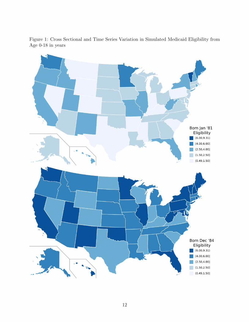
Figure 1: Cross Sectional and Time Series Variation in Simulated Medicaid Eligibility fromAge 0-18 in years
12
By studying the impact of Medicaid eligibility from birth to age 18 on long term outcomes
after age 18, we potentially mitigate concerns of legislative endogeneity relative to studies
that examine the impact of Medicaid eligibility at a point in time on contemporaneous
outcomes. The traditional legislative endogeneity concern is that states increase Medicaid
eligibility in response to changes in the outcomes of interest such that the results do not
reflect the causal policy impact. Similar concerns are still present in our analysis, but we
expect that they are at least weakly less severe than they are in contemporaneous analysis. In
contemporaneous analysis, there is a concern if states enact policy in response to outcomes at
a single point in time. In our analysis, for the legislative endogeneity concern to be as severe
as it is in contemporaneous specifications, states would have to enact policy in response to
outcomes at all points in time from birth to age 18.
4 Results
We present results for each of our five main outcomes from the tax data and our two main
outcomes from the MSIS data one at a time. For our tax outcome, we first consider OLS
results with no controls other than state and cohort fixed effects, which should be biased
toward showing deleterious impacts of Medicaid. We then present OLS results with the full
set of richer controls, which should be biased, but less so. Finally, we consider our preferred
instrumental variable estimates for all outcomes. We begin by presenting results pooled
across genders, and we also present separate results for women and men to allow for differ-
ential impacts given differential means. Our sample includes 4,911,040 female observations
and 5,129,194 male observations for outcomes through age 28.
4.1 Cumulative Income and Payroll Taxes
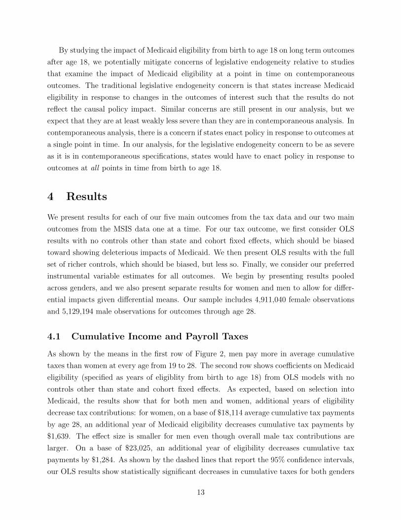
As shown by the means in the first row of Figure 2, men pay more in average cumulative
taxes than women at every age from 19 to 28. The second row shows coefficients on Medicaid
eligibility (specified as years of eligiblity from birth to age 18) from OLS models with no
controls other than state and cohort fixed effects. As expected, based on selection into
Medicaid, the results show that for both men and women, additional years of eligibility
decrease tax contributions: for women, on a base of $18,114 average cumulative tax payments
by age 28, an additional year of Medicaid eligibility decreases cumulative tax payments by
$1,639. The effect size is smaller for men even though overall male tax contributions are
larger. On a base of $23,025, an additional year of eligibility decreases cumulative tax
payments by $1,284. As shown by the dashed lines that report the 95% confidence intervals,
our OLS results show statistically significant decreases in cumulative taxes for both genders
13
at all ages.
The coefficients are still negative, though the coefficients are smaller in magnitude, when
we add our full set of controls to the OLS model. Even though we control very flexibly for
income using splines, we still see negative coefficients. Using this specification, we find that
an additional year of eligibility decreases average cumulative tax contributions at age 28 by
$292 among women and $259 among men. We see statistically significant decreases in tax
payments at all ages.
Turning to our simulated instrument specification in the last row of Figure 2, the coef-
ficients change sign. We find that Medicaid eligibility increases tax contributions for both
women and men, though the results are larger and more significant for women. The larger
tax impacts for women are consistent with the larger EITC and wage impacts for women
that we find below. By age 28, women have contributed an average of $18,114 in taxes and
each additional year of eligibility from birth to age 18 increases their cumulative tax payment
by $247. This result is statistically significant at the 1% level at ages 20-21 and 25-28 and
at the 5% level at ages 21-24, as shown in the last row of Figure 2.
By age 28, men have contributed an average of $23,025 in income and payroll taxes. The
point estimate suggests that each year of eligibility increases their cumulative contributions
by $127. This increase is about half as much as the increase for women, even though men
pay more in taxes overall. We observe positive impacts on cumulative taxes for men at
all ages, though we see less statistical significance for men. We see increases in cumulative
tax payments for men that are statistically significant at the 5% level at ages 19, 25, and
26. Pooling men and women, the IV coefficient shows that a one standard deviation in-
crease in Medicaid eligibility from birth to age 18 (an increase of 3.98 years of eligibility)
increases cumulative tax payments by age 28 by $740 (=186*3.98), which represents a 3.6%
(=740/20,623) increase.
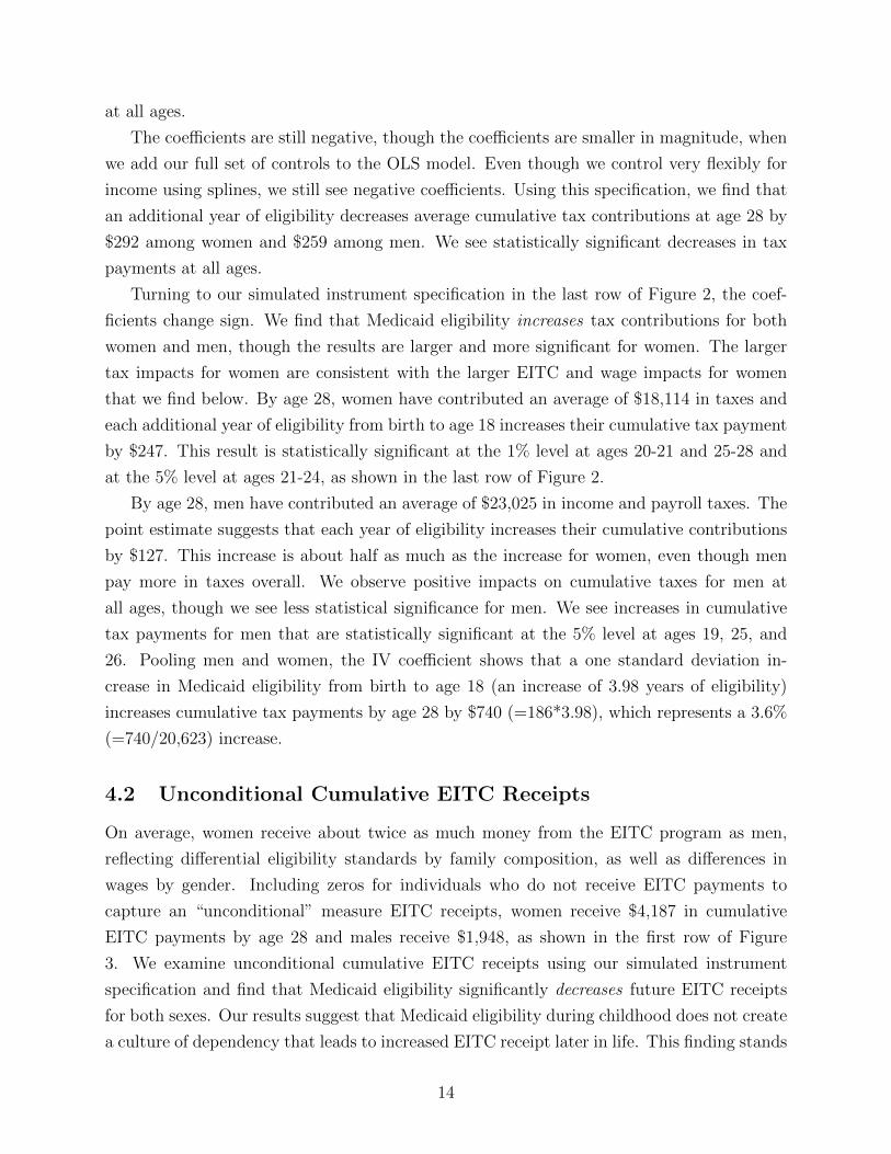
4.2 Unconditional Cumulative EITC Receipts
On average, women receive about twice as much money from the EITC program as men,
reflecting differential eligibility standards by family composition, as well as differences in
wages by gender. Including zeros for individuals who do not receive EITC payments to
capture an “unconditional” measure EITC receipts, women receive $4,187 in cumulative
EITC payments by age 28 and males receive $1,948, as shown in the first row of Figure
3. We examine unconditional cumulative EITC receipts using our simulated instrument
specification and find that Medicaid eligibility significantly decreases future EITC receipts
for both sexes. Our results suggest that Medicaid eligibility during childhood does not create
a culture of dependency that leads to increased EITC receipt later in life. This finding stands
14
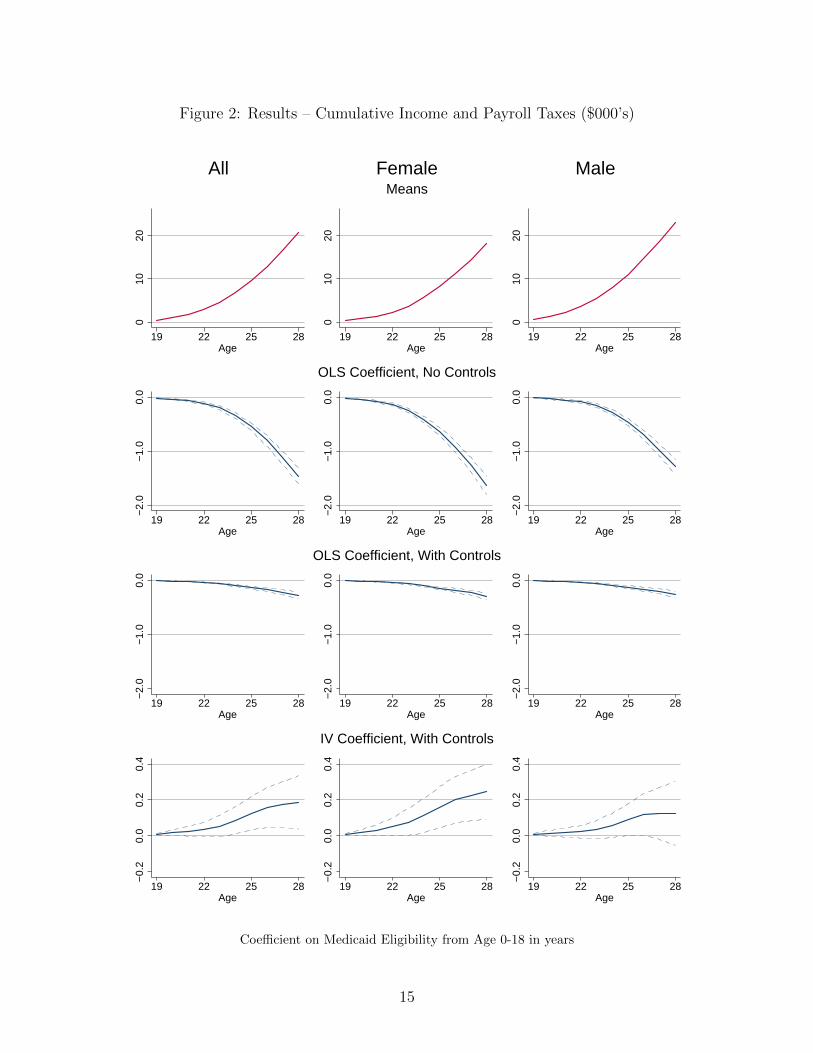
Figure 2: Results – Cumulative Income and Payroll Taxes ($000’s)
All Female Male
010
20
19 22 25 28Age
010
2019 22 25 28
Age
010
20
19 22 25 28Age
Means
−2.
0−
1.0
0.0
19 22 25 28Age
−2.
0−
1.0
0.0
19 22 25 28Age
−2.
0−
1.0
0.0
19 22 25 28Age
OLS Coefficient, No Controls
−2.
0−
1.0
0.0
19 22 25 28Age
−2.
0−
1.0
0.0
19 22 25 28Age
−2.
0−
1.0
0.0
19 22 25 28Age
OLS Coefficient, With Controls
−0.
20.
00.
20.
4
19 22 25 28Age
−0.
20.
00.
20.
4
19 22 25 28Age
−0.
20.
00.
20.
4
19 22 25 28Age
IV Coefficient, With Controls
Coefficient on Medicaid Eligibility from Age 0-18 in years
15

in contrast to findings from recent work by Dahl et al. (2013).
For each additional year of Medicaid eligibility from birth to age 18, women receive $109
less in cumulative EITC payments by age 28, as shown in the second row of Figure 3. Males
receive $41 less. These results are statistically significant for women at all ages and for men
at all ages after age 19.
In results not shown, we see that Medicaid eligibility has an impact on EITC receipt
through the participation margin. 51% of females participate in EITC at some point be-
tween age 19 and age 28, and a one standard deviation increase in their Medicaid eligibility
(3.99 years) results in a statistically significant 1.7% (=(0.22*3.99)/51) decrease in EITC
participation. Similarly, 44% of males participate in EITC at some point between age 19
and age 28, and a one standard deviation increase in their Medicaid eligibility (3.96 years)
results in a 1.5% (=(0.17*3.96)/44) decrease in EITC particpation. However, the male par-
ticipation result is not statistically different from zero.
We can compare our EITC results to our tax results to explore what fraction of the
increased taxes that we observe occurs as a result of decreased EITC payments. When
considering both males and females at age 28, an additional year of eligibility from birth to
age 18 increases cumulative tax payments by $186 and reduces cumulative EITC receipts by
$75. Therefore, around 40% of the observed increased tax payments occur through reductions
in EITC. The rest likely occurs because actual payments to the government increase when
wages and income increase. We next examine changes in wages directly.
4.3 Unconditional Cumulative Wages
We examine a measure of cumulative wages that is “unconditional” on working because we
include zero wages for individuals who do not work. Our simulated instrument coefficients,
presented in the bottom row of Figure 3, provide evidence that Medicaid eligibility has a
positive effect on future wages. On a base of $136,591 cumulative wages from age 19 to
28, the female point estimate suggests a $656 increase for each additional year of Medicaid
eligibility from birth to age 18. This result is statistically significant at the 5% level at age
28 and at many earlier ages.
Men enjoy higher average wages at every age, but there is less compelling evidence that
they experience increases in wages as a result of Medicaid eligibility. In fact, point estimates
at some ages are negative, and we observe a slight downward trend in the point estimates as
men age. On a base of $161,360 cumulative wages from age 19 to 28, the point estimate at
age 28 suggests a $134 decrease for each additional year of Medicaid eligibility from birth to
age 18. However, this decrease is not statistically significant. As shown by the dashed lines
that report the upper and lower bounds of the 95% interval in the bottom row of Figure 3, the
16
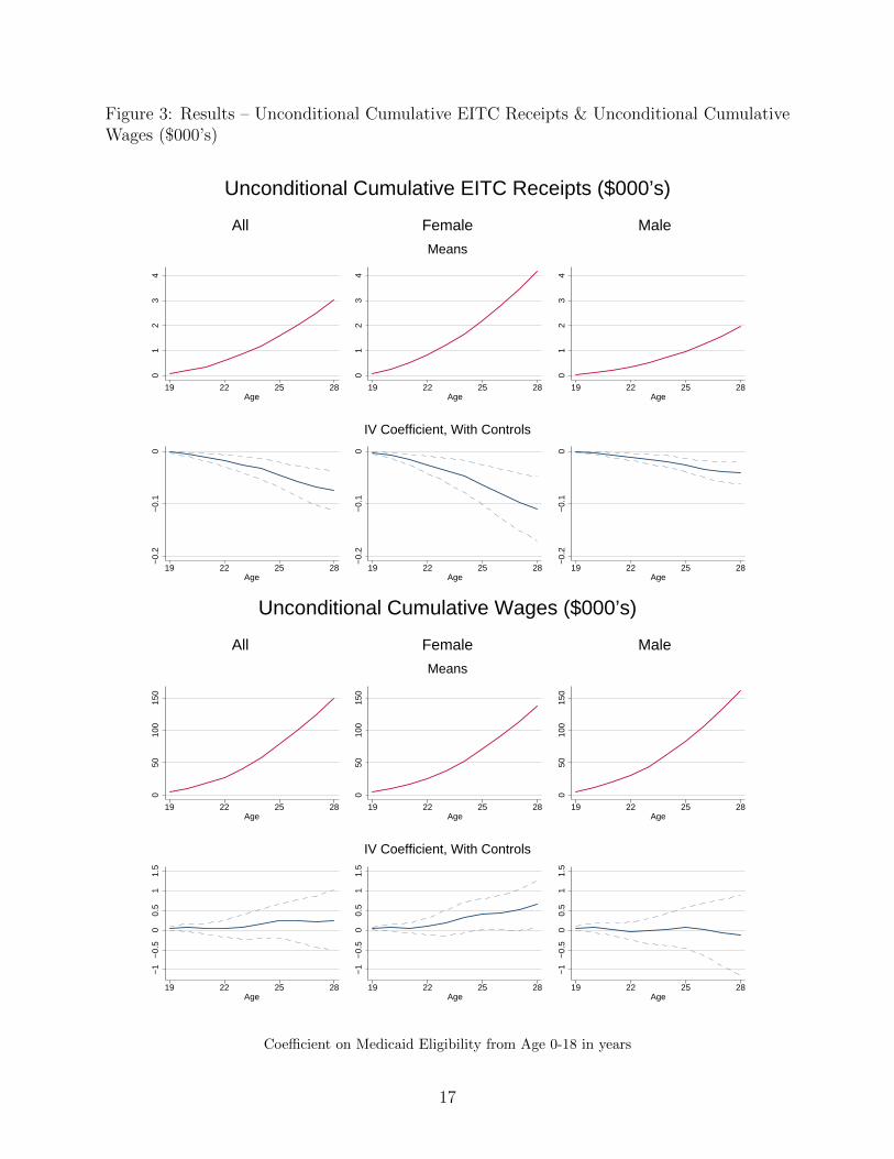
Figure 3: Results – Unconditional Cumulative EITC Receipts & Unconditional CumulativeWages ($000’s)
All Female Male
01
23
4
19 22 25 28Age
01
23
4
19 22 25 28Age
01
23
4
19 22 25 28Age
Means
−0.
2−
0.1
0
19 22 25 28Age
−0.
2−
0.1
0
19 22 25 28Age
−0.
2−
0.1
019 22 25 28
Age
IV Coefficient, With Controls
Unconditional Cumulative EITC Receipts ($000’s)
All Female Male
050
100
150
19 22 25 28Age
050
100
150
19 22 25 28Age
050
100
150
19 22 25 28Age
Means
−0.
50.
51.
5−
10
1
19 22 25 28Age
−0.
50.
51.
5−
10
1
19 22 25 28Age
−0.
50.
51.
5−
10
1
19 22 25 28Age
IV Coefficient, With Controls
Unconditional Cumulative Wages ($000’s)
Coefficient on Medicaid Eligibility from Age 0-18 in years
17
estimates for males are somewhat less precise than the estimates for females, likely driven
by higher variability in wages for males. In unreported results that consider cumulative
wages only for individuals with positive earnings, we draw very similar conclusions because
individuals of both genders have high rates of labor force participation.
To put our wage results for women in the context of a finding from the small existing
literature on long term wage impacts of interventions during childhood, Chetty et al. (2011)
find that a one standard deviation increase in teacher value-added in a given grade increases
earnings at age 28 by 1.3%. Our estimate of a one standard deviation increase in Medicaid
eligibility is of a similar magnitude. A one standard deviation increase in female Medicaid
eligibility (3.99 years) results in a 1.9% (=(656*3.99)/136,591) increase in cumulative earn-
ings by age 28. Incidentally, Chetty et al. (2011) also show that wages at age 28 are a good
predictor of future wages, which supports our focus on outcomes at age 28 in this paper.
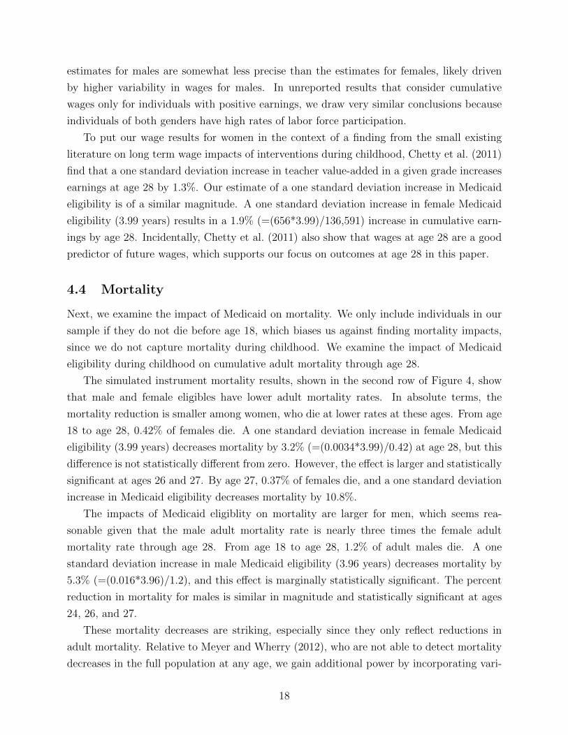
4.4 Mortality
Next, we examine the impact of Medicaid on mortality. We only include individuals in our
sample if they do not die before age 18, which biases us against finding mortality impacts,
since we do not capture mortality during childhood. We examine the impact of Medicaid
eligibility during childhood on cumulative adult mortality through age 28.
The simulated instrument mortality results, shown in the second row of Figure 4, show
that male and female eligibles have lower adult mortality rates. In absolute terms, the
mortality reduction is smaller among women, who die at lower rates at these ages. From age
18 to age 28, 0.42% of females die. A one standard deviation increase in female Medicaid
eligibility (3.99 years) decreases mortality by 3.2% (=(0.0034*3.99)/0.42) at age 28, but this
difference is not statistically different from zero. However, the effect is larger and statistically
significant at ages 26 and 27. By age 27, 0.37% of females die, and a one standard deviation
increase in Medicaid eligibility decreases mortality by 10.8%.
The impacts of Medicaid eligiblity on mortality are larger for men, which seems rea-
sonable given that the male adult mortality rate is nearly three times the female adult
mortality rate through age 28. From age 18 to age 28, 1.2% of adult males die. A one
standard deviation increase in male Medicaid eligibility (3.96 years) decreases mortality by
5.3% (=(0.016*3.96)/1.2), and this effect is marginally statistically significant. The percent
reduction in mortality for males is similar in magnitude and statistically significant at ages
24, 26, and 27.
These mortality decreases are striking, especially since they only reflect reductions in
adult mortality. Relative to Meyer and Wherry (2012), who are not able to detect mortality
decreases in the full population at any age, we gain additional power by incorporating vari-
18
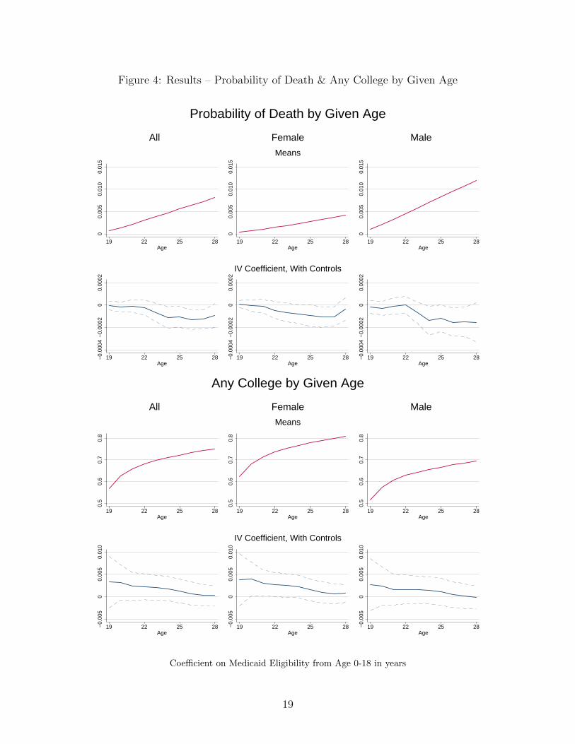
Figure 4: Results – Probability of Death & Any College by Given Age
All Female Male
0.00
50.
010
0.01
50
19 22 25 28Age
0.00
50.
010
0.01
50
19 22 25 28Age
0.00
50.
010
0.01
50
19 22 25 28Age
Means
−0.
0004
−0.
0002
0.00
020
19 22 25 28Age
−0.
0004
−0.
0002
0.00
020
19 22 25 28Age
−0.
0004
−0.
0002
0.00
020
19 22 25 28Age
IV Coefficient, With Controls
Probability of Death by Given Age
All Female Male
0.5
0.6
0.7
0.8
19 22 25 28Age
0.5
0.6
0.7
0.8
19 22 25 28Age
0.5
0.6
0.7
0.8
19 22 25 28Age
Means
−0.
005
0.00
50.
010
0
19 22 25 28Age
−0.
005
0.00
50.
010
0
19 22 25 28Age
−0.
005
0.00
50.
010
0
19 22 25 28Age
IV Coefficient, With Controls
Any College by Given Age
Coefficient on Medicaid Eligibility from Age 0-18 in years
19
ation in eligibility based on parental income and state of residence during childhood, which
are not available in their data. The decreases in mortality that we find, which could reflect
general improvements in health from childhood Medicaid eligibility, provide a suggestive
mechanism for our wage and tax results.
4.5 College Attendance
As the final outcome within our tax data, we consider the relationship between Medicaid
eligibility and college attendance. As shown in the first row of Figure 4, a larger percentage
of women than men have ever attended college at every age from 18 to 28.
Using our simulated instrument specification, as shown in the last row of Figure 4, we
find that both male and female Medicaid eligibles are more likely to have attended college.
This effect is more pronounced for women. The coefficients plotted in the bottom row show
that female eligibles are more likely to have attended college by any age, starting at age 19,
through age 28. The increase in college attendance is statistically different from zero at ages
20-22, an important age for college attendance. On a base of 68% of the female population
that has ever attended college by age 20, one additional year of eligibility from birth to age
18 increases the likelihood of having ever attended college by 0.40 percentage points. There
is suggestive evidence of increased college attendance among male Medicaid eligibles at age
20. Only 58% of the male population have ever attended college by age 20. The coefficient
suggests that one additional year of Medicaid eligibility increases the likelihood of having
ever attended college by 0.24 percentage points. As a percentage of mean college attendance,
the effect sizes for males are closer to the effect sizes for women, but they are still slightly
smaller. Like decreased mortality, increased college attendance could also potentially explain
some of the mechanism for our tax and wage outcomes.
4.6 Medicaid Spending and Return on Investment
Next, using data from the Medicaid Statistical Information System (MSIS), we calculate
the increase in Medicaid spending induced by the expansions that we study. In contrast to
the tax outcomes, we only run a single regression with spending as the dependent variable
because spending from birth to age 18 does not change after age 18. Furthermore, Medicaid
spending is not available separately for women and men, so we pool both genders.8 We report
the results in Table 1. When we apply a 3% discount rate, as shown in the top portion of
the first column, each additional year of Medicaid eligibility from birth to age 18 increases
8The MSIS does not report spending or take-up for Arizona in some years, so we drop observations forchildren who lived in Arizona in those years.
20
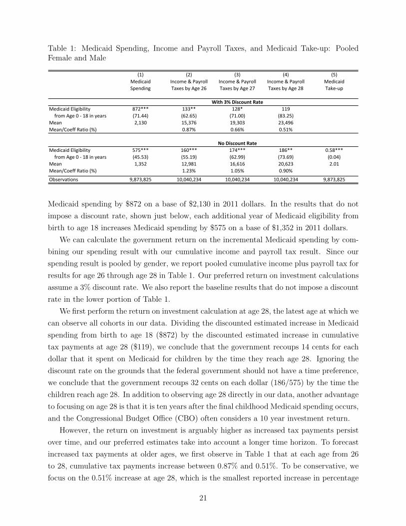
Table 1: Medicaid Spending, Income and Payroll Taxes, and Medicaid Take-up: PooledFemale and Male
(1) (2) (3) (4) (5)MedicaidSpending
Income & Payroll Taxes by Age 26
Income & Payroll Taxes by Age 27
Income & Payroll Taxes by Age 28
MedicaidTake-‐up
With 3% Discount RateMedicaid Eligibility 872*** 133** 128* 119from Age 0 -‐ 18 in years (71.44) (62.65) (71.00) (83.25)
Mean 2,130 15,376 19,303 23,496Mean/Coeff Ratio (%) 0.87% 0.66% 0.51%
No Discount RateMedicaid Eligibility 575*** 160*** 174*** 186** 0.58***from Age 0 -‐ 18 in years (45.53) (55.19) (62.99) (73.69) (0.04)
Mean 1,352 12,981 16,616 20,623 2.01Mean/Coeff Ratio (%) 1.23% 1.05% 0.90%
Observations 9,873,825 10,040,234 10,040,234 10,040,234 9,873,825
Medicaid spending by $872 on a base of $2,130 in 2011 dollars. In the results that do not
impose a discount rate, shown just below, each additional year of Medicaid eligibility from
birth to age 18 increases Medicaid spending by $575 on a base of $1,352 in 2011 dollars.
We can calculate the government return on the incremental Medicaid spending by com-
bining our spending result with our cumulative income and payroll tax result. Since our
spending result is pooled by gender, we report pooled cumulative income plus payroll tax for
results for age 26 through age 28 in Table 1. Our preferred return on investment calculations
assume a 3% discount rate. We also report the baseline results that do not impose a discount
rate in the lower portion of Table 1.
We first perform the return on investment calculation at age 28, the latest age at which we
can observe all cohorts in our data. Dividing the discounted estimated increase in Medicaid
spending from birth to age 18 ($872) by the discounted estimated increase in cumulative
tax payments at age 28 ($119), we conclude that the government recoups 14 cents for each
dollar that it spent on Medicaid for children by the time they reach age 28. Ignoring the
discount rate on the grounds that the federal government should not have a time preference,
we conclude that the government recoups 32 cents on each dollar (186/575) by the time the
children reach age 28. In addition to observing age 28 directly in our data, another advantage
to focusing on age 28 is that it is ten years after the final childhood Medicaid spending occurs,
and the Congressional Budget Office (CBO) often considers a 10 year investment return.
However, the return on investment is arguably higher as increased tax payments persist
over time, and our preferred estimates take into account a longer time horizon. To forecast
increased tax payments at older ages, we first observe in Table 1 that at each age from 26
to 28, cumulative tax payments increase between 0.87% and 0.51%. To be conservative, we
focus on the 0.51% increase at age 28, which is the smallest reported increase in percentage
21
terms. We assume that the increased tax payments persist as a percentage of mean tax
payments at every age going forward. To estimate mean tax payments by age, we take a
random sample of one in one thousand of tax returns in 2011 and calculate mean payments
and filing probabilities by age. Tax year 2011 was anomalous because of the payroll tax
holiday, so we calculate mean tax payments assuming that that there had been no payroll
tax holiday. Based on this calculation, we find that the government recoups 56 cents on the
dollar by age 60.
For comparison, we perform a similar return on investment calculation assuming a dis-
count rate of zero. As shown in the lower portion of Table 1, across ages 26 to 28, the
most conservative increase in cumulative tax payments is 0.90% on the age 28 base. Our
results change dramatically if we do not impose a discount rate: the government recoups its
investment by age 36 and by age 60, the government has earned a 550% return. We report
our results that impose a 3% discount rate as our main results because they are much more
conservative.
One caveat to our return on investment calculations is that our tax measure only includes
federal taxes, but the Medicaid spending includes state and federal spending. In practice, the
federal government paid for about 50% of Medicaid spending in the period that we study,
making the return on investment for the federal government even larger. However, given
that the federal government will pay almost the entire bill for Medicaid expansions under
the ACA, our calculation is relevant to those expansions.
4.7 Medicaid Take-up
Finally, using other data from MSIS, we examine the impact of Medicaid eligibility on take-
up of Medicaid. As shown in the last column of Table 1, Medicaid take-up increases by 0.58
years for each additional year of Medicaid eligibility from birth to age 18. We have previously
argued that we prefer estimates based on Medicaid eligibility instead of take-up, however,
it is interesting to examine Medicaid take-up to gauge the magnitudes of our results. Our
results imply that if we want to report impacts on beneficiaries as opposed to eligibles, we
should multiply all of our effect sizes by a factor of (1/0.5804), which is approximately 1.7.
For example, our tax results imply that for each additional year of Medicaid enrollment from
birth to age 18, cumulative tax payments at age 28 increase by $321.04 (=186.331*1.723).
5 Variation that Drives the Results
To illustrate the variation in simulated Medicaid eligibility that drives our results and its
relationship with our outcomes of interest, we perform a novel exercise. The goal of this
22

exercise is to demonstrate which cohorts and states give the most identifying variation and
to show a graphical dose-response relationship between this identifying variation and our
outcomes of interest. Identification in our main specifications exists at the cohort (month of
birth from January 1981 to December 1984) by state level. For children who move between
states during their childhoods, the instrument reflects the vector of state policies to which
they are exposed, but we abstract away from that variation in this exercise.
For this exercise, we eliminate variation in our instrument, first by cohort, and then by
state, to determine whether variation across states or variation across cohorts is empirically
more relevant for our main IV results. Next, using variation only across states, we graph
the first stage and reduced form for each cohort. Analogously, using variation only across
cohorts, we graph the first stage and reduced form for each state. In these graphs, we look
for a dose-response relationship that suggests that greater changes in medicaid eligibility
lead to greater changes in adult outcomes, which we would expect to find in the case of
homogeneous treatment effects.
First, we eliminate variation by cohort such that variation only exists across states.
Using the entire estimation sample, we average the values of the instrument∑18
t=0 Ics,a=t
by state at age 15 such that we obtain a new instrument∑18
t=0 Is,a=t that only varies across
states. Similarly, using the entire estimation sample, we average the values of the instrument∑18t=0 Ics,a=t by cohort such that we obtain a new instrument
∑18t=0 Ic,a=t that only varies
across cohorts. Next, we run our main IV specification given by Equations 1 and 2 with our
new instruments (one at a time) in place of the full instrument. In the specification where
the instrument only varies across states, we must drop the state fixed effects. Similarly, in
the specification where the instrument only varies across cohorts, we must drop the fixed
effects by cohort, but we can and do still include fixed effects by birth year. Below, we
separately investigate cohort variation across and within birth years.
As shown in Table 1, our IV coefficient in our main specification is 186, which indicates
that an additional year of Medicaid eligibility during childhood increases cumulative income
and payroll tax payments at age 28 by $186 on a base of $20,623 in 2011 dollars. In the
analogous specification in which we only use variation across states, we obtain a larger
coefficient which indicates an increase in payroll and income payments by age 28 by $915 on
the same base. This coefficient is statistically different from zero at the 1% level. However,
when we only use variation across cohorts, controlling for year of birth, we obtain a negative
coefficient which indicates a decrease in cumulative income and payroll tax payments of
$2,432 on the same base, and this coefficient is statistically different from zero at the 1%
level. This comparison tells us that variation across states drives our finding that Medicaid
eligibility increases tax payments at age 28, and variation across cohorts works against it.
23
Next, we dig deeper, asking which cohorts experience the largest variation across states.
We run a separate first stage regression using data from each cohort k separately, identified
only by variation across states:
18∑t=0
Mis,c=k,a=t = δk18∑t=0
Is,a=t +Xi,a=15 + ηi. (3)
This equation is related to the baseline first stage equation given by Equation 2, but note
that it no longer includes state fixed effects γs,a=15 because the variation now exists at the
state level. It also no longer includes cohort fixed effects γc because each regression only
includes data from a single cohort k. From these regressions, we obtain a coefficient δk for
each cohort. This coefficient gives us the magnitude of the change in Medicaid eligibility
identified only by variation across states within each cohort.
We can compare the magnitudes of these coefficients across cohorts to determine which
cohorts exhibit the most variation in Medicaid eligibility across states through the simu-
lated instrument. We find a coefficient δk of 0.9 for our oldest cohort, born January 1981,
which indicates that each additional year of simulated eligibility translates into 0.9 years of
eligibility for this cohort. In contrast, we find a larger coefficient δk of 1.4 for our youngest
cohort, born December 1984, indicating that variation in generosity across states leads to
more variation in Medicaid eligibility in the youngest cohort than it does in the oldest co-
hort. Averaging the first stage coefficients across all cohorts born in the same calendar year,
weighting by the observation count, we find a general pattern that the first stage across states
increases as birth year increases from µδ,k∈1981 = 0.88 to µδ,k∈1982 = 1.03 to µδ,k∈1983 = 1.16
to µδ,k∈1984 = 1.32. This pattern is not surprising, given that Medicaid eligibility increased
over time.
The same pattern generally holds within each birth year, with children born in later
months of the year experiencing greater first stage variation than children born in earlier
months of the year, also because younger cohorts generally have greater Medicaid eligibility.
The horizontal axis of Figure 5 depicts variation in the first stage coefficient within each birth
year by normalizing the coefficient by the observation-weighted average coefficient from that
calendar year. As shown, the first stage coefficient is strikingly larger for children born in
October, November, and December of the 1983 cohort relative to children born in earlier
months of the same year. This pattern reflects the federal legislation that differentially
affected children born after September 30, 1983, discussed above.
Next, we examine whether larger first stage variation translates into larger reduced form
variation in outcomes. Simulated Medicaid eligibility could have heterogeneous treatment
effects on different cohorts, so there is no reason to expect an exact linear relationship
24
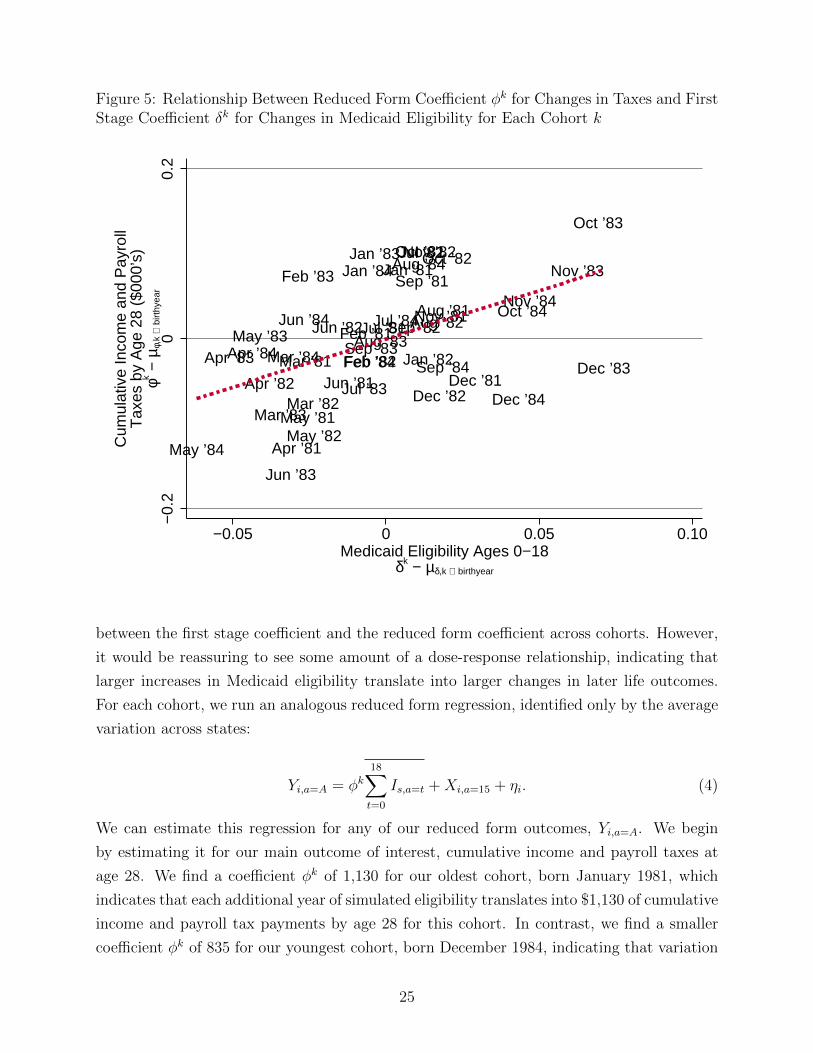
Figure 5: Relationship Between Reduced Form Coefficient φk for Changes in Taxes and FirstStage Coefficient δk for Changes in Medicaid Eligibility for Each Cohort k
Jan ’81Oct ’81
Nov ’81
Dec ’81
Feb ’81
Mar ’81
Apr ’81
May ’81
Jun ’81
Jul ’81Aug ’81
Sep ’81
Jan ’82Feb ’82
Mar ’82Apr ’82
May ’82
Jun ’82
Jul ’82
Aug ’82Sep ’82
Oct ’82Nov ’82
Dec ’82
Jan ’83Feb ’83
Mar ’83
Apr ’83May ’83
Jun ’83
Jul ’83
Aug ’83Sep ’83
Oct ’83
Nov ’83
Dec ’83
Jan ’84
Feb ’84Mar ’84Apr ’84
May ’84
Jun ’84 Jul ’84
Aug ’84
Sep ’84
Oct ’84Nov ’84
Dec ’84
−0.
20.
20
Cum
ulat
ive
Inco
me
and
Pay
roll
Tax
es b
y A
ge 2
8 ($
000’
s)φk −
µφ,
k ∈
birt
hyea
r
−0.05 0.05 0.100Medicaid Eligibility Ages 0−18
δk − µδ,k ∈ birthyear
between the first stage coefficient and the reduced form coefficient across cohorts. However,
it would be reassuring to see some amount of a dose-response relationship, indicating that
larger increases in Medicaid eligibility translate into larger changes in later life outcomes.
For each cohort, we run an analogous reduced form regression, identified only by the average
variation across states:
Yi,a=A = φk18∑t=0
Is,a=t +Xi,a=15 + ηi. (4)
We can estimate this regression for any of our reduced form outcomes, Yi,a=A. We begin
by estimating it for our main outcome of interest, cumulative income and payroll taxes at
age 28. We find a coefficient φk of 1,130 for our oldest cohort, born January 1981, which
indicates that each additional year of simulated eligibility translates into $1,130 of cumulative
income and payroll tax payments by age 28 for this cohort. In contrast, we find a smaller
coefficient φk of 835 for our youngest cohort, born December 1984, indicating that variation
25
in generosity across states increases tax payments in the oldest cohort more than it does
in the youngest cohort. Indeed, averaging the reduced form coefficients across all cohorts
born in the same calendar year, weighting by the observation count, we find a general
pattern that the reduced form decreases as the birth year increases from µφ,k∈1981 = 1, 048
to µφ,k∈1982 = 1, 032 to µφ,k∈1983 = 976 to µφ,k∈1984 = 907.
If we simply relate the average first stage coefficient for each year of birth to the average
reduced form coefficient for each year of birth, we find a negative relationship between Medi-
caid eligibility and cumulative income and payroll taxes. We also see a negative relationship
if we relate the first stage to the reduced form by cohort without regard to birth year. These
results are consistent with the negative coefficient that we obtain in the full specification
above that only uses variation across cohorts. However, our attempt to eliminate time ef-
fects by examining all cohorts at the same age could still allow for time to have a differential
impact on individuals born in different calendar years through mechanisms such as business
cycles which affect different cohorts in the same year but at different ages. It is especially
important to take calendar years into account given that we only observe adult outcomes
once per calendar year at tax time.
The vertical axis of Figure 5 depicts variation in the reduced form coefficient within
each birth year by demeaning the coefficient by the observation-weighted-average coefficient
within each calendar year of birth. Each point gives (δk − µδ,k∈birthyear, φk − µφ,k∈birthyear) for
a single cohort, identified only by variation across states. As shown, within each birth year,
children born in later months have larger tax payments by age 28. Strikingly, children born
in October 1983, the youngest affected by the federal Medicaid expansion, have the largest
increases in cumulative income and payroll taxes, suggesting that increases in Medicaid
eligibility are indeed the mechanism for larger income and payroll taxes.
The dashed line in Figure 5 gives the observation-weighted average relationship between
the first stage and reduced form coefficients demeaned by year of birth. The upward slope
shows that larger increases in Medicaid eligibility identified by average variation across states
translate into larger increases in tax payments by age 28. The slope of the line, which is 1, 135,
is itself an instrumental variable estimate because it gives the change in the reduced form
in response to the change in the first stage. This slope is a difference-in-difference estimate
of sorts, which uses variation across states to identify a coefficient within each cohort and
then compares coefficients across cohorts. It indicates that if we increase Medicaid eligibility
during childhood by one year, cumulative income and payroll taxes at age 28 increase by
$1,135. This slope is similar in magnitude to the $915 coefficient that we obtained in the
full instrumental variable specification that uses only variation across states.
We next perform the analogous exercise, using only variation across cohorts within states.
26
Using the entire estimation sample, we average the values of the instrument∑18
t=0 Ics,a=t by
state such that the new instrument∑18
t=0 Ic,a=t only exists at the cohort level. Next, we run
a separate first stage regression using data from state x separately, identified only by the
average variation across cohorts:
18∑t=0
Mic,s=x,a=t = δx18∑t=0
Ic,a=t + birthyearc +Xi,a=15 + ηi. (5)
This first stage equation is related to the baseline stage equation given by Equation 2, but it
no longer includes state fixed effects γs,a=15 because each regression only includes data from
a single cohort. It also no longer includes cohort fixed effects γc because the variation now
exists at the cohort level, so they would drop out of the regression. However, we can and
do include fixed effects by calendar year of birth birthyearc so that we take into account
that reduced form outcomes are measured in different tax years for children born in different
calendar years.
Next, we run a separate reduced form regression using data from state x separately,
identified only by the average variation across cohorts:
Yi,a=A = φx18∑t=0
Ic,a=t + birthyearc +Xi,a=15 + ηi. (6)
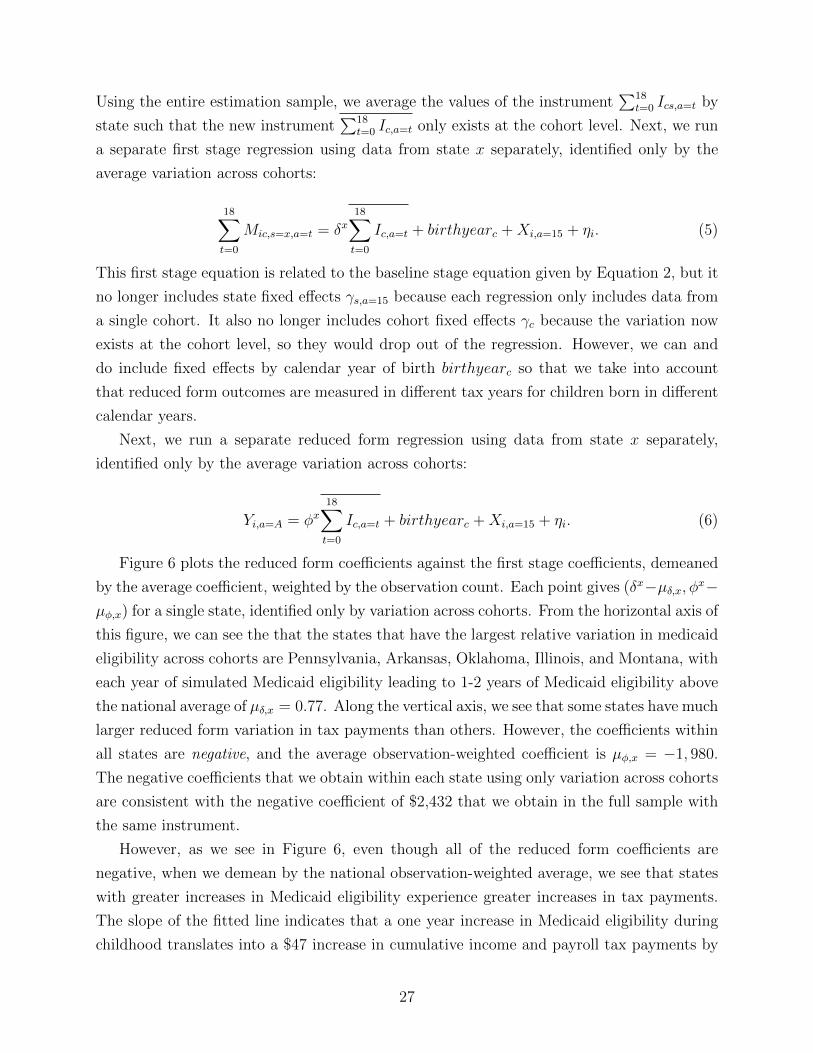
Figure 6 plots the reduced form coefficients against the first stage coefficients, demeaned
by the average coefficient, weighted by the observation count. Each point gives (δx−µδ,x, φx−µφ,x) for a single state, identified only by variation across cohorts. From the horizontal axis of
this figure, we can see the that the states that have the largest relative variation in medicaid
eligibility across cohorts are Pennsylvania, Arkansas, Oklahoma, Illinois, and Montana, with
each year of simulated Medicaid eligibility leading to 1-2 years of Medicaid eligibility above
the national average of µδ,x = 0.77. Along the vertical axis, we see that some states have much
larger reduced form variation in tax payments than others. However, the coefficients within
all states are negative, and the average observation-weighted coefficient is µφ,x = −1, 980.
The negative coefficients that we obtain within each state using only variation across cohorts
are consistent with the negative coefficient of $2,432 that we obtain in the full sample with
the same instrument.
However, as we see in Figure 6, even though all of the reduced form coefficients are
negative, when we demean by the national observation-weighted average, we see that states
with greater increases in Medicaid eligibility experience greater increases in tax payments.
The slope of the fitted line indicates that a one year increase in Medicaid eligibility during
childhood translates into a $47 increase in cumulative income and payroll tax payments by
27
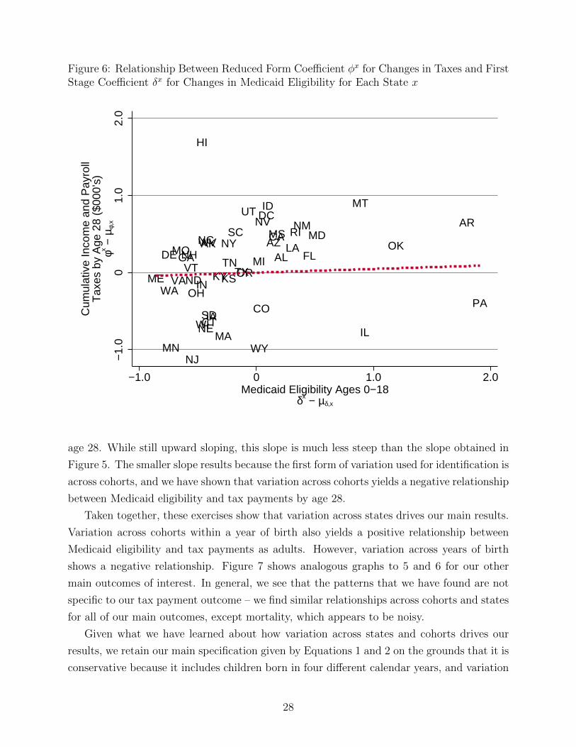
Figure 6: Relationship Between Reduced Form Coefficient φx for Changes in Taxes and FirstStage Coefficient δx for Changes in Medicaid Eligibility for Each State x
AKAL
AR
AZCA
COCT
DC
DE FLGA
HI
IA
ID
IL
IN KSKY
LA
MA
MD
ME
MI
MN
MO
MS
MT
NC
ND
NE
NH
NJ
NMNV
NY
OH
OK
OR
PA
RISC
SD
TNTX
UT
VAVT
WA
WI
WV
WY
−1.
01.
02.
00
Cum
ulat
ive
Inco
me
and
Pay
roll
Tax
es b
y A
ge 2
8 ($
000’
s)φx −
µφ,
x
−1.0 1.0 2.00Medicaid Eligibility Ages 0−18
δx − µδ,x
age 28. While still upward sloping, this slope is much less steep than the slope obtained in
Figure 5. The smaller slope results because the first form of variation used for identification is
across cohorts, and we have shown that variation across cohorts yields a negative relationship
between Medicaid eligibility and tax payments by age 28.
Taken together, these exercises show that variation across states drives our main results.
Variation across cohorts within a year of birth also yields a positive relationship between
Medicaid eligibility and tax payments as adults. However, variation across years of birth
shows a negative relationship. Figure 7 shows analogous graphs to 5 and 6 for our other
main outcomes of interest. In general, we see that the patterns that we have found are not
specific to our tax payment outcome – we find similar relationships across cohorts and states
for all of our main outcomes, except mortality, which appears to be noisy.
Given what we have learned about how variation across states and cohorts drives our
results, we retain our main specification given by Equations 1 and 2 on the grounds that it is
conservative because it includes children born in four different calendar years, and variation
28
Figure 7: Relationship Between Reduced Form Coefficients φk, φx for Outcomes and FirstStage Coefficients δk, δx for Changes in Medicaid Eligibilty for Each Cohort k and for EachState x
Jan ’81
Oct ’81Nov ’81
Dec ’81
Feb ’81Mar ’81
Apr ’81May ’81
Jun ’81Jul ’81Aug ’81
Sep ’81Jan ’82
Feb ’82
Mar ’82Apr ’82
May ’82
Jun ’82Jul ’82
Aug ’82
Sep ’82Oct ’82
Nov ’82Dec ’82
Jan ’83
Feb ’83
Mar ’83Apr ’83
May ’83
Jun ’83
Jul ’83Aug ’83
Sep ’83 Oct ’83
Nov ’83Dec ’83
Jan ’84
Feb ’84Mar ’84
Apr ’84May ’84
Jun ’84Jul ’84
Aug ’84
Sep ’84Oct ’84Nov ’84
Dec ’84
−0.
050.
050
Unc
ondi
tiona
l Cum
ulat
ive
EIT
C b
y A
ge 2
8 ($
000’
s)φk −
µφ,
k ∈
birt
hyea
r
−0.05 0.05 0.100
AK
AL
AR
AZ
CA
CO
CT
DC
DE FLGAHIIA ID
IL
IN
KSKYLA
MA MDMEMIMN
MO
MS
MT
NC
NDNE
NH
NJ
NM
NV
NYOH OK
OR PARI
SC
SD
TNTX
UT
VA VTWAWI
WV
WY
−0.
20.
20
Unc
ondi
tiona
l Cum
ulat
ive
EIT
C b
y A
ge 2
8 ($
000’
s)φx −
µφ,
x
−0.5 0.5 1.0 1.50
Jan ’81
Oct ’81
Nov ’81
Dec ’81
Feb ’81Mar ’81
Apr ’81May ’81
Jun ’81Jul ’81
Aug ’81
Sep ’81
Jan ’82Feb ’82
Mar ’82
Apr ’82May ’82
Jun ’82Jul ’82
Aug ’82Sep ’82
Oct ’82
Nov ’82
Dec ’82
Jan ’83Feb ’83
Mar ’83
Apr ’83
May ’83Jun ’83Jul ’83
Aug ’83
Sep ’83
Oct ’83
Nov ’83
Dec ’83Jan ’84Feb ’84
Mar ’84Apr ’84
May ’84
Jun ’84
Jul ’84Aug ’84
Sep ’84
Oct ’84Nov ’84
Dec ’84
−1.
01.
00
Unc
ondi
tiona
l Cum
ulat
ive
Wag
es b
y A
ge 2
8 ($
000’
s)φk −
µφ,
k ∈
birt
hyea
r
−0.05 0.05 0.100
AK
ALAR
AZCA
COCT
DC
DE
FLGA
HI
IA
ID
IL
IN KSKY
LA
MA
MD
MEMI
MN
MO MSMTNC
ND
NE
NH
NJ
NM
NVNY
OH
OK
OR PA
RI
SC
SD
TNTX
UTVA VT
WAWI
WV
WY−5
510
0
Unc
ondi
tiona
l Cum
ulat
ive
Wag
es b
y A
ge 2
8 ($
000’
s)φx −
µφ,
x
−0.5 0.5 1.0 1.50
Jan ’81
Oct ’81
Nov ’81
Dec ’81
Feb ’81
Mar ’81
Apr ’81
May ’81
Jun ’81Jul ’81
Aug ’81
Sep ’81Jan ’82Feb ’82Mar ’82
Apr ’82
May ’82
Jun ’82
Jul ’82Aug ’82
Sep ’82
Oct ’82Nov ’82Dec ’82
Jan ’83
Feb ’83
Mar ’83
Apr ’83
May ’83
Jun ’83
Jul ’83
Aug ’83Sep ’83
Oct ’83
Nov ’83Dec ’83
Jan ’84
Feb ’84
Mar ’84
Apr ’84May ’84Jun ’84Jul ’84
Aug ’84
Sep ’84
Oct ’84
Nov ’84
Dec ’84
−0.
0005
0.00
050
Pro
babi
lity
of D
eath
by A
ge 2
8φk −
µφ,
k ∈
birt
hyea
r
−0.05 0.05 0.100
AK
AL AR
AZ CACO
CT
DC
DEFLGAHIIA ID IL
IN
KSKY
LA
MAMD
ME
MI
MN
MO
MS
MT
NC
ND
NE NHNJ
NM
NVNYOH OKOR
PARI
SC
SDTNTX UT
VA
VT
WA
WIWV
WY
−0.
002
0.00
20.
004
0
Pro
babi
lity
of D
eath
by A
ge 2
8φx −
µφ,
x
−0.5 0.5 1.0 1.50
Jan ’81
Oct ’81
Nov ’81
Dec ’81
Feb ’81Mar ’81Apr ’81
May ’81
Jun ’81
Jul ’81Aug ’81
Sep ’81
Jan ’82Feb ’82
Mar ’82Apr ’82May ’82Jun ’82
Jul ’82
Aug ’82
Sep ’82
Oct ’82
Nov ’82
Dec ’82Jan ’83
Feb ’83Mar ’83
Apr ’83May ’83
Jun ’83
Jul ’83
Aug ’83Sep ’83
Oct ’83
Nov ’83Dec ’83
Jan ’84Feb ’84Mar ’84
Apr ’84
May ’84Jun ’84
Jul ’84
Aug ’84
Sep ’84Oct ’84Nov ’84
Dec ’84
−0.
002
0.00
20.
004
0
Any
Col
lege
Atte
ndan
ceby
Age
28
φk − µ
φ,k
∈ b
irthy
ear
−0.05 0.05 0.100Medicaid Eligibility Ages 0−18
δk − µδ,k ∈ birthyear
AK
AL
AR
AZCACO
CT
DC
DEFL
GA
HI
IA
ID
ILIN
KS
KY LA
MAMD
ME
MIMNMO
MS
MT
NC
ND
NE
NH
NJ
NM
NV
NYOH
OK
ORPA
RISC
SDTN
TX
UT
VA
VT
WA
WI
WV
WY
−0.
010.
010
Any
Col
lege
Atte
ndan
ceby
Age
28
φx − µ
φ,x
−0.5 0.5 1.0 1.50Medicaid Eligibility Ages 0−18
δx − µδ,x
29
across calendar years severely attenuates our results. If we estimate our main specification
using data from each calendar year separately, such that variation only comes from the
vector of childhood states and the month of birth within a calendar year, we see a positive
relationship between Medicaid eligibility and our main tax outcome of interest within each
birth year, with an additional year of Medicaid eligibility leading to increased cumulative
tax payments by age 28 of $871 for children born in 1981, $875 for children born in 1982,
$82 for children born in 1983, and $533 for children born in 1984. Our main IV coefficient
is $186, which is smaller than the coefficients for all but one of the birth years. Notably, the
coefficient for the 1983 birth year is the smallest, even though the federal legislation induces
the most variation across cohorts within the 1983 birth year. All-in-all, though variation
across cohorts born in 1983 works in the same direction as our main results, our main results
rely on variation across states. Variation across birth years attenuates our results.
Given what we have learned about variation across birth years, it is also conservative
for us to focus on outcomes at age 28 as opposed to focusing on outcomes at later ages.
Figure A1 shows IV coefficients from ages 19 to 31 for all of our main outcomes of interest,
and Figure A2 shows the corresponding means. Although the corresponding means for all
outcomes increase smoothly with age, the IV coefficients increase dramatically in absolute
magnitude for ages 29 to 31 relative to earlier ages. Our analysis in this section explains
the dramatic increase in magnitude. Because variation across years of birth attenuates our
results, when we remove years of birth, our results increase in magnitude. While we can
observe all four years of birth (1981-1984) at age 28, we can only observe three years of birth
(1981-1983) at age 29, two years of birth (1981-1982) at age 30, and one year of birth (1981)
at age 31. Not surprisingly, our results are much larger at older ages. Our main coefficient
suggests that each year of Medicaid eligibility during childhood increases cumulative income
and payroll taxes at age 31 by $1,561 on a base of $35,268, a 4.4% increase. Therefore,
focusing on results at age 28 is conservative.
The exercise that we have performed here to explore variation in our instrument could
be useful in other applications where the instrument varies along two dimensions. The key
novel feature of this exercise is that we first eliminate variation along one dimension to focus
only on variation along the other dimension. If we had not done so and had simply run our
main specification restricting our sample to single states or single month of birth cohorts,
it would not have been as informative to compare the magnitudes of the first stage and
reduced form coefficients along the other dimension because the first stage coefficients would
have approached one within each group. Using a fixed instrument for all groups allows us
to compare first stage and reduced form magnitudes across groups and to conclude that
variation across states drives our results much more than variation across cohorts.
30
6 Robustness
To examine the sensitivity of our results to our main sample selection restriction, we impute
Medicaid eligibility for individuals in the tax years in which their parents do not file taxes
and incorporate these “non-filers” into our regression sample. To ensure that our estimate of
the impact of Medicaid is conservative, we assume that all children are eligible for Medicaid
in the years when their parents do not file. We generally think of the filing threshold as
around the poverty level, so non-filing occurs when parents fall below the poverty level, and
many, but not all, children will be eligible for Medicaid if their parents do not file. For these
non-filers, we set simulated eligibility equal to the average value of the instrument for filers
in the same birth cohort and state at age 15 (which is itself sometimes imputed).9 Using
our main tax outcome, we find results that are similar in magnitude to our main results. As
shown in Figure A3, by age 28, the average individual has contributed $19,037 in income and
payroll taxes, and each additional year of eligibility increases the cumulative contribution by
$157 (which is slightly larger than the $119 increase on a larger base in the main sample).
This estimate and all other estimates from ages 19-28 are statistically significant at least
the 10% level. As with our main results, the increase in cumulative tax payments is more
pronounced for females and less pronounced for males, further demonstrating the robustness
of our results to the inclusion of non-filers.
7 Conclusion
There has been very little work on the long-term impact of Medicaid expansions, or the long-
term impact of most interventions, for that matter, because of data availability. However,
beyond data availability, studying long-term impacts brings unique challenges. Perhaps the
biggest challenge is that between the intervention and the long term, other interventions
can occur, so it is difficult to assess whether the apparent impact is actually the result of
the initial intervention or the impact of subsequent interventions. This issue is particularly
prevalent in the case of Medicaid expansions because Medicaid expansions tend to occur
by state, and states that expand Medicaid in one year could expand it further in future
years. By focusing on Medicaid expansions in the 1980’s and 1990’s, we can follow the same
individual in our longitudinal tax data to generate a measure of Medicaid eligibility in each
year that is arguably one of the most accurate and representative ever generated.
Looking forward to the implementation of the Affordable Care Act, our research suggests
9We need to impute values for several of the control variables, including state at age 15, number of siblingsat age 15, and family income at age 15. We impute these values using the values from the closest availablefiling year, and we also include a control for non-filing.
31
that Medicaid generally has favorable effects on eligible children. We find that by expanding
Medicaid to children, the government recoups much of its investment over time in the form of
higher future tax payments. Moreover, children exposed to Medicaid collect less money from
the government in the form of the Earned Income Tax Credit, and the women have higher
cumulative earnings by age 28. Aside from the positive return on the government investment,
the eligible children themselves also experience decreases in mortality and increases in college
attendance.
References
Katherine Baicker, Amy Finkelstein, Jae Song, and Sarah Taubman. The impact of medicaid
on labor force and program participation: Evidence from the oregon health insurance
experiment. NBER Working Paper 19547, October 2013a.
Katherine Baicker, Sarah Taubman, Heidi L. Allen, Mira Bernstein, Jonathan Gruber,
Joseph P. Newhouse, Eric C. Schneider, Bill J. Wright, Alan M. Zaslavsky, and Amy N.
Finkelstein. The oregon experiment - effects of medicaid on clinical outcomes. New Eng-
land Journal of Medicine, 368(18):1713–1722, 2013b. doi: 10.1056/NEJMsa1212321.
Cynthia Bansak and Steven Raphael. The effect of state policy design features on take up
and crowd out rates for the state children’s health insurance program. Journal of Policy
Analysis and Management, 26(1):149–175, 2006.
Linda J Blumberg, Lisa Dubay, and Stephen A Norton. Did the medicaid expansions for
children displace private insurance? an analysis using the SIPP. Journal of Health Eco-
nomics, 19(1):33 – 60, 2000. doi: http://dx.doi.org/10.1016/S0167-6296(99)00020-X. URL
http://www.sciencedirect.com/science/article/pii/S016762969900020X.
George Borjas. Welfare reform, labor supply, and health insurance in the immigrant popu-
lation. Journal of Health Economics, 22(5):933–958, 2003. URL http://www.jstor.org/
stable/3211795.
Michel H. Boudreaux. The long-term effects of exposure to medicaid in early childhood,
2014. URL http://conservancy.umn.edu/handle/11299/165384.
Thomas C. Buchmueller, Lo Sasso Anthony T., and Wong Kathleen N. How did SCHIP
affect the insurance coverage of immigrant children? The B.E. Journal of Economic
Analysis & Policy, 8(2):1–25, 2008.
32
David Card and Lara D. Shore-Sheppard. Using discontinuous eligibility rules to identify
the effects of the federal medicaid expansions on low-income children. The Review of
Economics and Statistics, 86(3):752–766, 2004. URL http://www.jstor.org/stable/
3211795.
Raj Chetty, John N. Friedman, Nathaniel Hilger, Emmanuel Saez, Diane Whitmore Schazen-
bach, and Danny Yagan. How does your kindergarten classroom affect your earnings?
evidence from project star. Quarterly Journal of Economics, 126(4):1593–1660, 2011.
Raj Chetty, John N. Friedman, and Emmanuel Saez. Using differences in knowledge across
neighborhoods to uncover the impacts of the eitc on earnings. American Economic Review,
103(7):2683–2721, 2013a. doi: 10.1257/aer.103.7.2683. URL http://www.aeaweb.org/
articles.php?doi=10.1257/aer.103.7.2683.
Sarah Cohodes, Samuel A. Kleiner, Michael Lovenheim, and Dan Grossman. The effect of
child health insurance access on schooling: Evidence from public insurance expansions.
NBER Working Paper No. w20178, May 2014.
Peter J. Cunningham, Jack Hadley, and James Reschovsky. The effects of SCHIP on chil-
dren’s health insurance coverage: Early evidence from the community tracking study.
Medical Care Research and Review, 59(4):359–383, 2002a. doi: 10.1177/107755802237807.
Peter J. Cunningham, James Reschovsky, and Jack Hadley. SCHIP, medicaid expansions lead
to shifts in children’s coverage. Issue Brief: Center for Studying Health System Change,
59:1–6, 2002b.
Janet Currie and Jonathan Gruber. Health insurance eligibility, utilization of medical care,
and child health. The Quarterly Journal of Economics, 111(2):431–466, 1996a. doi: 10.
2307/2946684.
Janet Currie and Jonathan Gruber. Saving babies: The efficacy and cost of recent expansions
of medicaid eligibility for pregnant women. Journal of Political Economy, 104(6):1263–
1296, 1996b. URL http://www.jstor.org/stable/2138939.
Gordon B. Dahl, Andreas Ravndal Kostol, and Magne Mogstad. Family welfare cultures.
NBER Working Paper 19237, 2013.
Dhaval Dave, Sandra Decker, Robert Kaestner, and Kosali Ilayperuma Simon. The effect
of medicaid expansions in the late 1980s and early 1990s on the labor supply of pregnant
women. NBER Working Paper No. w19161, 2013.
33
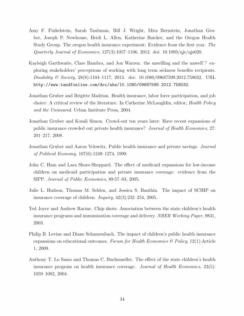
Amy F. Finkelstein, Sarah Taubman, Bill J. Wright, Mira Bernstein, Jonathan Gru-
ber, Joseph P. Newhouse, Heidi L. Allen, Katherine Baicker, and the Oregon Health
Study Group. The oregon health insurance experiment: Evidence from the first year. The
Quarterly Journal of Economics, 127(3):1057–1106, 2012. doi: 10.1093/qje/qjs020.
Kayleigh Garthwaite, Clare Bambra, and Jon Warren. the unwilling and the unwell’? ex-
ploring stakeholders’ perceptions of working with long term sickness benefits recipients.
Disability & Society, 28(8):1104–1117, 2013. doi: 10.1080/09687599.2012.758032. URL
http://www.tandfonline.com/doi/abs/10.1080/09687599.2012.758032.
Jonathan Gruber and Brigitte Madrian. Health insurance, labor force participation, and job
choice: A critical review of the literature. In Catherine McLaughlin, editor, Health Policy
and the Uninsured. Urban Institute Press, 2004.
Jonathan Gruber and Kosali Simon. Crowd-out ten years later: Have recent expansions of
public insurance crowded out private health insurance? Journal of Health Economics, 27:
201–217, 2008.
Jonathan Gruber and Aaron Yelowitz. Public health insurance and private savings. Journal
of Political Economy, 107(6):1249–1274, 1999.
John C. Ham and Lara Shore-Sheppard. The effect of medicaid expansions for low-income
children on medicaid participation and private insurance coverage: evidence from the
SIPP. Journal of Public Economics, 89:57–83, 2005.
Julie L. Hudson, Thomas M. Selden, and Jessica S. Banthin. The impact of SCHIP on
insurance coverage of children. Inquiry, 42(3):232–254, 2005.
Ted Joyce and Andrew Racine. Chip shots: Association between the state children’s health
insurance programs and immunization coverage and delivery. NBER Working Paper, 9831,
2003.
Philip B. Levine and Diane Schanzenbach. The impact of children’s public health insurance
expansions on educational outcomes. Forum for Health Economics & Policy, 12(1):Article
1, 2009.
Anthony T. Lo Sasso and Thomas C. Buchmueller. The effect of the state children’s health
insurance program on health insurance coverage. Journal of Health Economics, 23(5):
1059–1082, 2004.
34
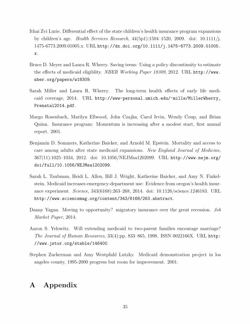
Ithai Zvi Lurie. Differential effect of the state children’s health insurance program expansions
by children’s age. Health Services Research, 44(5p1):1504–1520, 2009. doi: 10.1111/j.
1475-6773.2009.01005.x. URL http://dx.doi.org/10.1111/j.1475-6773.2009.01005.
x.
Bruce D. Meyer and Laura R. Wherry. Saving teens: Using a policy discontinuity to estimate
the effects of medicaid eligiblity. NBER Working Paper 18309, 2012. URL http://www.
nber.org/papers/w18309.
Sarah Miller and Laura R. Wherry. The long-term health effects of early life medi-
caid coverage, 2014. URL http://www-personal.umich.edu/~mille/MillerWherry_
Prenatal2014.pdf.
Margo Rosenbach, Marilyn Ellwood, John Czajka, Carol Irvin, Wendy Coup, and Brian
Quinn. Insurance program: Momentum is increasing after a modest start, first annual
report. 2001.
Benjamin D. Sommers, Katherine Baicker, and Arnold M. Epstein. Mortality and access to
care among adults after state medicaid expansions. New England Journal of Medicine,
367(11):1025–1034, 2012. doi: 10.1056/NEJMsa1202099. URL http://www.nejm.org/
doi/full/10.1056/NEJMsa1202099.
Sarah L. Taubman, Heidi L. Allen, Bill J. Wright, Katherine Baicker, and Amy N. Finkel-
stein. Medicaid increases emergency-department use: Evidence from oregon’s health insur-
ance experiment. Science, 343(6168):263–268, 2014. doi: 10.1126/science.1246183. URL
http://www.sciencemag.org/content/343/6168/263.abstract.
Danny Yagan. Moving to opportunity? migratory insurance over the great recession. Job
Market Paper, 2014.
Aaron S. Yelowitz. Will extending medicaid to two-parent families encourage marriage?
The Journal of Human Resources, 33(4):pp. 833–865, 1998. ISSN 0022166X. URL http:
//www.jstor.org/stable/146400.
Stephen Zuckerman and Amy Westpfahl Lutzky. Medicaid demonstration project in los
angeles county, 1995-2000 progress but room for improvement. 2001.
A Appendix
35
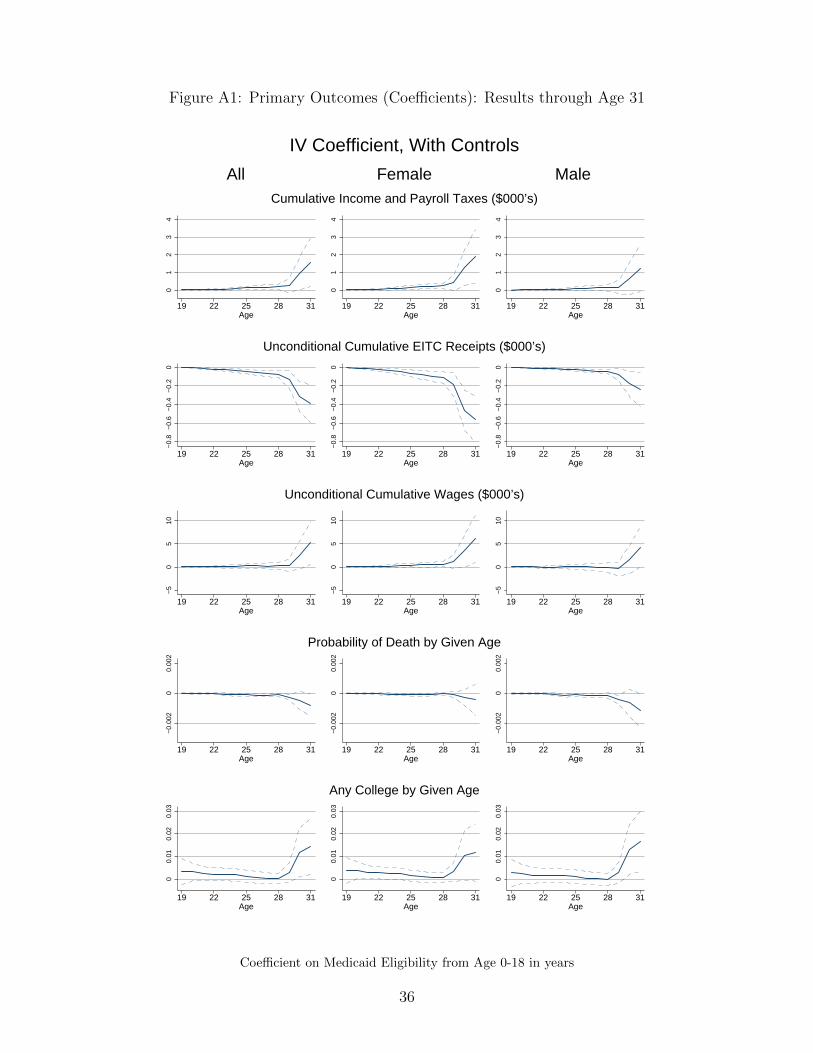
Figure A1: Primary Outcomes (Coefficients): Results through Age 31
All Female Male0
12
34
19 22 25 28 31Age
01
23
4
19 22 25 28 31Age
01
23
4
19 22 25 28 31Age
Cumulative Income and Payroll Taxes ($000’s)
−0.
8−
0.6
−0.
4−
0.2
0
19 22 25 28 31Age
−0.
8−
0.6
−0.
4−
0.2
0
19 22 25 28 31Age
−0.
8−
0.6
−0.
4−
0.2
0
19 22 25 28 31Age
Unconditional Cumulative EITC Receipts ($000’s)
−5
05
10
19 22 25 28 31Age
−5
05
10
19 22 25 28 31Age
−5
05
10
19 22 25 28 31Age
Unconditional Cumulative Wages ($000’s)
−0.
002
0.00
20
19 22 25 28 31Age
−0.
002
0.00
20
19 22 25 28 31Age
−0.
002
0.00
20
19 22 25 28 31Age
Probability of Death by Given Age
0.01
0.02
0.03
0
19 22 25 28 31Age
0.01
0.02
0.03
0
19 22 25 28 31Age
0.01
0.02
0.03
0
19 22 25 28 31Age
Any College by Given Age
IV Coefficient, With Controls
Coefficient on Medicaid Eligibility from Age 0-18 in years
36
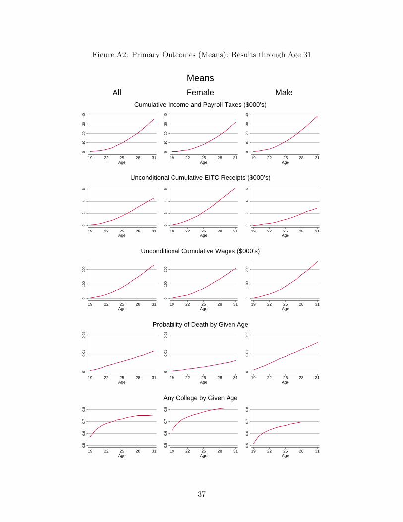
Figure A2: Primary Outcomes (Means): Results through Age 31
All Female Male0
1020
3040
19 22 25 28 31Age
010
2030
40
19 22 25 28 31Age
010
2030
40
19 22 25 28 31Age
Cumulative Income and Payroll Taxes ($000’s)
02
46
19 22 25 28 31Age
02
46
19 22 25 28 31Age
02
46
19 22 25 28 31Age
Unconditional Cumulative EITC Receipts ($000’s)
010
020
0
19 22 25 28 31Age
010
020
0
19 22 25 28 31Age
010
020
0
19 22 25 28 31Age
Unconditional Cumulative Wages ($000’s)
0.01
0.02
0
19 22 25 28 31Age
0.01
0.02
0
19 22 25 28 31Age
0.01
0.02
0
19 22 25 28 31Age
Probability of Death by Given Age
0.5
0.6
0.7
0.8
19 22 25 28 31Age
0.5
0.6
0.7
0.8
19 22 25 28 31Age
0.5
0.6
0.7
0.8
19 22 25 28 31Age
Any College by Given Age
Means
37
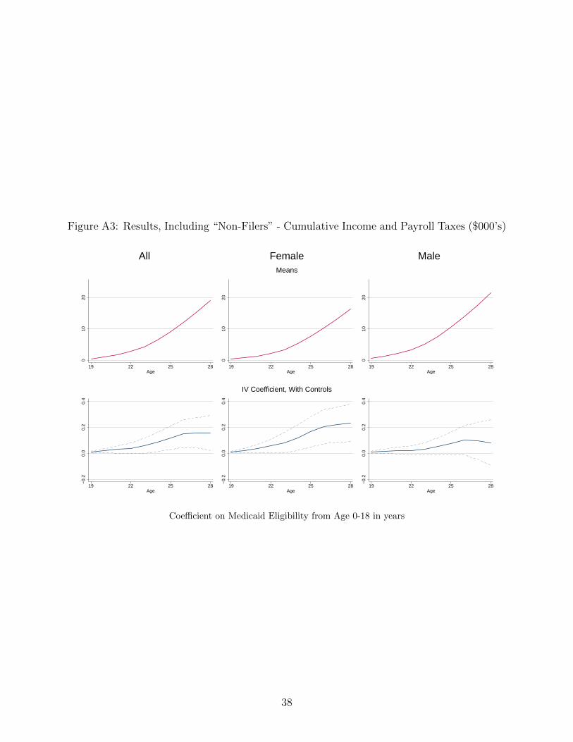
Figure A3: Results, Including “Non-Filers” - Cumulative Income and Payroll Taxes ($000’s)
All Female Male
010
20
19 22 25 28Age
010
20
19 22 25 28Age
010
2019 22 25 28
Age
Means
−0.
20.
00.
20.
4
19 22 25 28Age
−0.
20.
00.
20.
4
19 22 25 28Age
−0.
20.
00.
20.
4
19 22 25 28Age
IV Coefficient, With Controls
Coefficient on Medicaid Eligibility from Age 0-18 in years
38